the Creative Commons Attribution 4.0 License.
the Creative Commons Attribution 4.0 License.
 | 07 Apr 2022
Drone-based magnetic and multispectral surveys to develop a 3D model for mineral exploration at Qullissat, Disko Island, Greenland
Robert Jackisch
Björn H. Heincke
Robert Zimmermann
Erik V. Sørensen
Markku Pirttijärvi
Moritz Kirsch
Heikki Salmirinne
Stefanie Lode
Urpo Kuronen
Richard Gloaguen
Mineral exploration in the West Greenland flood basalt province is attractive because of its resemblance to the magmatic sulfide-rich deposit in the Russian Norilsk region, but it is challenged by rugged topography and partly poor exposure for relevant geologic formations. On northern Disko Island, previous exploration efforts have identified rare native iron occurrences and a high potential for Ni–Cu–Co–PGE–Au mineralization. However, Quaternary landslide activity has obliterated rock exposure in many places at lower elevations. To augment prospecting field work under these challenging conditions, we acquire high-resolution magnetic and multispectral remote sensing data using drones in the Qullissat area. From the data, we generate a detailed 3D model of a mineralized basalt unit, belonging to the Asuk Member of the Palaeocene Vaigat Formation.
Different types of legacy data and newly acquired geo- and petrophysical as well as geochemical-mineralogical measurements form the basis of an integrated geological interpretation of the unoccupied aerial system (UAS) surveys. In this context, magnetic data aim to define the location and the shape of the buried magmatic body, and to estimate if its magnetic properties are indicative for mineralization. UAS-based multispectral orthomosaics are used to identify surficial iron staining, which serves as a proxy for outcropping sulfide mineralization. In addition, UAS-based digital surface models are created for geomorphological characterization of the landscape to accurately reveal landslide features.
UAS-based magnetic data suggest that the targeted magmatic unit is characterized by a pattern of distinct positive and negative magnetic anomalies. We apply a 3D magnetization vector inversion (MVI) model to the UAS-based magnetic data to estimate the magnetic properties and shape of the magmatic body. By means of introducing constraints in the inversion, (1) UAS-based multispectral data and legacy drill cores are used to assign significant magnetic properties to areas that are associated with the mineralized Asuk Member, and (2) the Earth's magnetic and the palaeomagnetic field directions are used to evaluate the general magnetization direction in the magmatic units.
Our results suggest that the geometry of the mineralized target can be estimated as a horizontal sheet of constant thickness, and that the magnetization of the unit has a strong remanent component formed during a period of Earth's magnetic field reversal. The magnetization values obtained in the MVI are in a similar range to the measured ones from a drillcore intersecting the targeted unit. Both the magnetics and topography confirm that parts of the target unit were displaced by landslides. We identified several fully detached and presumably rotated blocks in the obtained model. The model highlights magnetic anomalies that correspond to zones of mineralization and is used to identify outcrops for sampling. Our study demonstrates the potential and efficiency of using high-resolution UAS-based multi-sensor data to constrain the geometry of partially exposed geological units and assist exploration targeting in difficult or poorly exposed terrain.
- Article
(34864 KB) - Full-text XML
- BibTeX
- EndNote


The volcanic rocks of Palaeocene age exposed on Disko-Nuussuaq in central-west Greenland form part of the North Atlantic Igneous Province (Larsen et al., 2016). Due to a similar geological setting the Disko-Nuussuaq area is regarded as analogous to the Norilsk–Talnakh Ni–Cu district in the Siberian trap basalt, and thus a highly prospective region for major Ni–Cu–Co platinum group element (PGE) deposits (Lightfoot et al., 1997; Keays and Lightfoot, 2007). Mineral exploration in the onshore parts of the basin at Disko Island and the Nuussuaq Peninsula dates back more than half a century (Pauly, 1958; Bird and Weathers, 1977; Ulff-Møller, 1990), and currently there are 12 active mineral exploration licences that cover an area of ∼ 10 000 km2 on Disko-Nuussuaq (Government of Greenland, 2021).
Large parts of the northern Disko region provide good outcrop conditions at the high plateau steep slopes, whereas the lower slopes near the coast are covered by debris from Quaternary rock falls, landslides, periglacial deposits and solifluction lobes (Pedersen et al., 2017). This incapacitates ground-based mineral exploration mapping efforts, which is further complicated by rugged topography and the Arctic climate.
Here, high-resolution, multi-parameter three-dimensional models are highly useful to resolve detailed structures and develop exploration models. This has traditionally been achieved by combining results from various exploration techniques (Vallée et al., 2011), with magnetics as one of the prime methods (Nabighian et al., 2005). Systematic airborne geophysics (Brethes et al., 2014, 2018) and remote sensing (Bedini, 2011; Bedini and Rasmussen, 2018) have been used in Greenland to create the uniform physical data basis for such modelling.
The recent development of small-scale unoccupied aerial systems (UASs) equipped with versatile sensors created a powerful tool in spatial mapping (Ren et al., 2019). Magnetic sensors (Gavazzi et al., 2016, 2019; Malehmir et al., 2017; Parshin et al., 2018; Walter et al., 2020; Zheng et al., 2021), as well as multi- and hyperspectral sensors (Kirsch et al., 2018; Jackisch et al., 2019; Booysen et al., 2020), on UASs make it possible to acquire data inexpensively and with higher resolution as compared to traditional airborne surveys. Magnetic data are suited to map surface and shallow subsurface structures (Le Maire et al., 2020) and are useful to reveal magnetized rock units and the location of sulfides and iron oxides (Gunn and Dentith, 1997). Integrated high-resolution red–green–blue (RGB) and image spectroscopy is employed to detect small-scale mineralization traces and can safely guide ground teams during exploration (Park and Choi, 2020).
Ground-based measurements and rock sampling are typically carried out as part of a mineral exploration campaign to establish and validate relationships between data measured from indirect airborne and UAS-based survey methods, and the field-based mineralogical, lithological and structural data. In addition, geomorphologic properties, e.g. the topography of landslides, can be incorporated in the geological interpretation. The tracing of mineralized boulders to discover in situ mineralization (colloquial: boulder hunting) is regarded as an effective exploration tool (Plouffe et al., 2011).
Landslide geohazard monitoring using UAS is an additional source of valuable data. In the Disko–Nuussuaq region, monitoring has received increased attention lately, highlighting the Nuussuaq basin as a risk area (Dahl-Jensen et al., 2004; Svennevig, 2019). Landslide descriptors (e.g. headscarps) are often hard to identify visually, because their characteristic appearance (e.g. fracture patterns) are eroded or overprinted by continuing mass movements.
In this study, we focus on an area south of Qullissat on the northern shore of Disko Island (Fig. 1), which has seen modern exploration since the early 1990s. Legacy data include airborne magnetic and active electromagnetic (EM) data as well as petrophysical data from six drillholes intersecting a magmatic body (Olshefsky, 1992; Olshefsky and Jerome, 1993, 1994; Olshefsky et al., 1995).
Apart from the airborne EM data, which were lacking parameter information to conduct an inversion, all data were available to the authors in limited quality. However, considering the limited thickness of the mineralized unit, and the lithological complexity of the area due to secondary mass movements, the data coverage of the legacy geophysical surveys is too coarse to develop a 3D exploration model of the area. Additionally, large rotated blocks may occur at coastal zones or are partially buried by talus.
We complement the existing data with newly acquired high-resolution drone, or UAS-based multi-sensor data. Magnetic measurements were carried out with a fixed-wing UAS (Jackisch et al., 2019, 2020) at low altitude and with dense line spacing to acquire high-resolution magnetic data. In addition, we conducted a high-resolution UAS-based multispectral and photogrammetry survey in order to create a precise elevation model and to systematically identify locations with increased iron content for mineralization vectoring. UAS-based data were supplemented with ground-based observations, magnetic surveys, handheld spectroscopy and magnetic susceptibility measurements as well as laboratory petrophysical and mineralogical analysis of rock samples from one legacy drill core from the area.
We link topography, surface mineralogy and the magnetic data to provide both direct and indirect information about potentially sulfide-enriched targets. In particular, we use the magnetic data in a constrained 3D magnetization vector inversion (MVI), including measured petrophysical properties, as a means to constrain the shape of the mineralized body and its main magnetization directions and distribution. Finally, results from all UAS and ground-based data are combined in a joint interpretation of the Qullissat area. The interpretation aims (1) to define and pinpoint potential exploration areas, and additionally (2) to determine where parts of the targeted magmatic unit are displaced by landslides.
1.1 Regional geological setting
The volcano-sedimentary Nuussuaq Basin in western Greenland formed as a rift basin in Early Cretaceous time during rifting of the Labrador Sea–Davis Strait area (Henderson et al., 1981; Chalmers et al., 1999; Dam et al., 2009). Because of the Neogene uplift (Japsen et al., 2005; Bonow et al., 2006), parts of the basin are now exposed in the onshore areas of Disko Island and Nuussuaq Peninsula in central West Greenland. The area is made up of Cretaceous to Palaeocene siliciclastic sediments of the Nuussuaq Group (Dam et al., 2009, and references therein) and Palaeogene volcanic rocks of the West Greenland Basalt Group (Pedersen et al., 2018, and references therein). On a regional scale, sediments were deposited in a deltaic environment in the eastern part of the basin (sandstones interbedded with mudstones), while deep marine sediments were deposited in the western part. During Late Cretaceous to Early Palaeocene rifting, sediments were block-rotated and eroded prior to the onset of volcanism (Chalmers et al., 1999; Dam et al., 2009).
The volcanism started in a submarine environment within the actively subsiding Nuussuaq Basin. Early eruptive products were hyaloclastites extruded from eruption centres located to the NW of Disko and Nuussuaq. With the volcanic build-up on the seafloor, volcanic islands were formed and over time volcanism became dominantly subaerial.
The Palaeocene volcanic succession is divided into a lower (Vaigat Formation) and an upper formation (Maligât Formation), which make up the bulk of the volcanic rocks exposed on Disko and Nuussuaq (Fig. 1b). The early volcanism of the Vaigat Formation was dominated by picritic rocks that erupted in three overall volcanic cycles (Larsen and Pedersen, 2009). The picritic rocks formed from melts generated through partial melting in the asthenosphere. The melts subsequently ascended through the crust and erupted at the surface without much interaction while traversing the crust from source to surface. However, throughout the volcanic pile intervals, crustally contaminated siliceous basalts to magnesian andesites occur (Larsen and Pedersen, 2009; Pedersen et al., 2017, 2018) indicating that primary magmas at certain times got contaminated in relatively high-level magma chambers. This is evidenced by the occurrence of partly digested shale and sandstone xenoliths in the volcanic rocks (Pedersen, 1977, 1985; Ulff-Møller, 1977).
1.2 Economic mineral potential
The economic mineral potential of the West Greenland Basalt Province is speculated to be an equivalent of the Norilsk-Talnakh region with potential for major Cu, Ni, Co and PGE deposits (Keays and Lightfoot, 2007; Rosa et al., 2013). Key similarities are a high proportion of high-temperature picritic lavas and a significant volume of sediment-contaminated basalts (Lightfoot and Hawkesworth, 1997).
When primary magmas passed through the sediments en route to the surface, they reacted at various locations with sedimentary successions modifying the chemical composition of the magmas. The rare native (telluric) iron is observed at several places across Disko and Nuussuaq (Ulff-Møller, 1985, 1990). It is commonly suggested that it is formed by the reaction of iron present in the magma with carbonaceous sediments (e.g. marine mudstone, deltaic shales, coal seams) resulting in extremely reducing environments leading to the precipitation of nickel-ferrous minerals and metallic iron (Howarth et al., 2017; Pedersen et al., 2017; Pernet-Fisher et al., 2017).
Under similar conditions, contamination from sulfur-rich sediments is also responsible for the precipitation of Ni, Cu, Co and PGE as immiscible sulfide droplets within the silicate magma that are scavenged and deposited (Sørensen et al., 2013).
At Illukunnguaq, north-eastern Disko, a massive 28 t Ni–Cu–Co–PGE boulder was discovered and had been investigated since 1870 (Steenstrup, 1901). At Hammer Dal, north-western part of Disko Island, a massive 10 t native-iron boulder was found in Stordal in 1985 (Ulff-Møller, 1986). These boulders indicate that processes leading to massive accumulations of iron-oxide and sulfide mineralization have occurred. In a dynamic open magmatic system, where a large volume of mafic nickel-rich melt streams through dykes and sills, huge Ni–Cu–PGE deposits (conduit type nickel deposit) can be formed. A common intrusive geometry found in large igneous provinces (LIPs) are extensive networks of tabular or saucer-shaped sills linked by dykes, which interact with the sedimentary basin (Barnes et al., 2016). A recent geochemical soil survey, an extended mobile metal ion study (Blue Jay Mining PLC, 2021), provided further indications of economic Ni–Cu–Co–PGE–Au deposits. In addition, significant amounts of Au were reported in native iron cumulate within one core sample (drillhole FP94-4-5) near Qullissat (4.8–38.3 g t−1 Au; Olshefsky et al., 1995), although the Au content was otherwise low and sporadic in further core samples.
Our main target is a sub-horizontal magmatic body that is located near Qullissat, about 20 km south-east of the well-investigated native-iron-bearing Asuk locality (Pedersen, 1985), and 25 km NW of the known Illukunnguaq Ni–Cu dyke (Pauly, 1958). Our target was first described as a sill called “Qullissat sill” (Olshefsky and Jerome, 1994; Pedersen et al., 2017). It is assumed to be part of the Vaigat Formation and quite similar to Asuk Member in chemical composition. The presence of sulfides, graphite and native iron in the intrusion (Olshefsky et al., 1995), which are all considered to be conductive, complicates an interpretation that is largely based on electromagnetic data. Detailed magnetic data can provide insight into which components are mainly responsible for conductivity anomalies, because graphite is non-magnetic but conductive, while pyrrhotite is quite magnetic (Gunn and Dentith, 1997). The observed native iron might have significant ferromagnetic properties (Nagata et al., 1970).
1.3 Geochronology and magnetic polarity of the basalt members
Previous palaeomagnetic investigations of volcanic strata on Disko and Nuussuaq (Deutsch and Kristjansson, 1974; Athavale and Sharma, 1975; Riisager and Abrahamsen, 1999, and references therein) showed that a geomagnetic pole reversal took place at ∼ 60.92 Ma (magnetochron C27n–C26r; Cande and Kent, 1995). About two-thirds of the lower–middle Vaigat Formation are normally polarized, but its upper third and the overlying Maligât Formation are reversely polarized.
Of importance to this paper is the Asuk Member, which formed during a period of reverse polarization shortly after the C27n–C26 pole reversal (Pedersen et al., 2017). Adjacent field measurements of the remanent magnetic field near the Asuk locality are available ∼ 25 km NW of Qullissat at sampling altitudes between 365–1450 m. Field declinations (D) between 123–154∘ and an inclination (I) of about −73∘ were reported (Athavale and Sharma, 1975). Remanent magnetic measurements were also reported from age-equivalent rocks of the Naujánguit Member at Qunnilik on southern Nuussuaq (Riisager and Abrahamsen, 1999, 2000), about 60 km north-west of Qullissat, where a reverse polarization with and D=228.1∘ were measured.
1.4 The Qullissat study area
The study area is located near the abandoned coal mining town Qullissat (70.0844∘ N, 53.0097∘ W) on the north coast of Disko Island (Fig. 1). The study area is ∼ 6 km long, ∼ 3 km wide and extends from sea level up to the steep Inussuk cliff (∼ 600–900 m above sea level (a.s.l.); Fig. 2). The lower parts of the study area (up to 600 m a.s.l.) are broadly debris and vegetation covered, affected by mass-movement and thus only show limited outcrops. The general geology of the area (Fig. 1c) is described on the official geological map and in more detail, in a photogrammetric cross section covering the area (see Pedersen et al. 2017, Fig. 161, p. 180).
The lower coastal cliffs (<100 m a.s.l.) are made up of Cretaceous sandstones with shale beds and coal seams of the Atane Formation, while scattered outcrops in the area up to 400 m a.s.l. are generally mapped as undifferentiated volcanic rocks or intrusions of iron and native iron-bearing magnesian andesite of the Asuk Member (Pedersen et al., 2017). Although originally described as a sill, recent investigations of the drillcores intersecting the area suggest that the intrusion might be an extrusive lava flow (personal communication with Asger Pedersen, Geological Survey of Denmark and Greenland GEUS, 2020).
The area from ∼ 400–600 m a.s.l. is characterized by landslide material from the lower Rinks Dal Member of the Maligât Formation. The uppermost part of the study area (∼ 600–900 m a.s.l.) consists of volcanic rocks of the Maligât Formation (Skarvefjeld Unit) that form the Inussuk cliff above the Qullissat area. The location of the magmatic plumbing system and the eruption centres for the Asuk Member lavas at Qullissat is unknown. However, considering the viscous nature of the Asuk Member, the andesitic magma lavas presumably did not spread far from their eruption site.
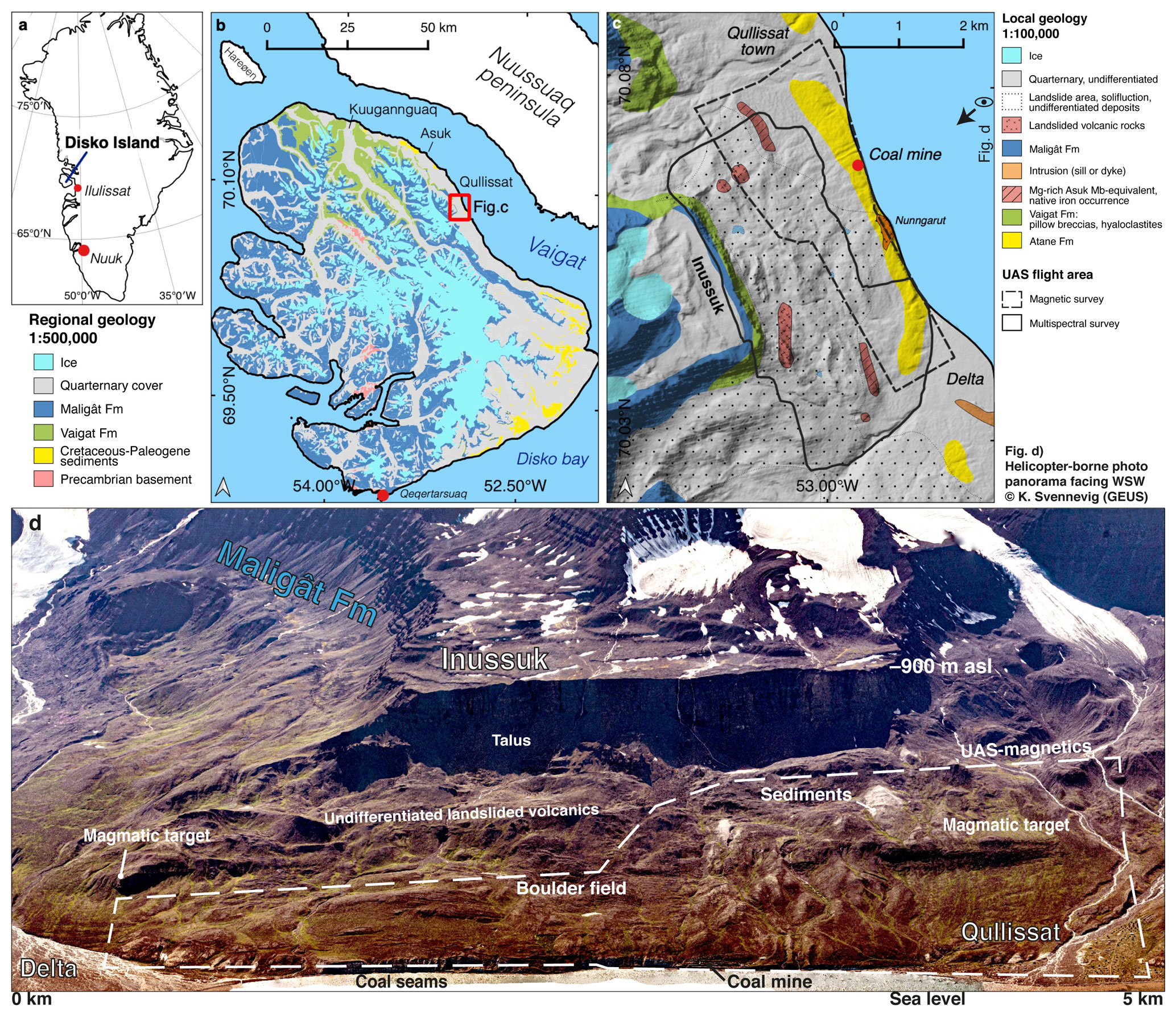
Figure 1General overview of the study area on northern Disko in West Greenland. (a) The Qullissat study area is located about 125 km NW of the village Ilulissat. (b) Regional geological map from Disko Island with the Palaeogene basaltic Maligât and Vaigat formations, which are emplaced in a Cretaceous sediment basin and incised deeply by glacial erosion. (c) Geological map of the survey site from this study at Qullissat (modified after Pedersen et al., 2013). (d) Oblique overview of the study area based on stitched helicopter-based RGB photographs. The horizontal distance at coast level is about 5 km and the Inussuk plateau is located at ∼ 900 m a.s.l.
1.5 Former exploration data
During the last few decades, multiple mineral exploration datasets were acquired within the study area (Olshefsky, 1992; Olshefsky and Jerome, 1993, 1994; Olshefsky et al., 1995; Data et al., 2005). Six holes were drilled (Olshefsky et al., 1995) by Falconbridge Greenland Ltd. in 1993 and 1994 (see locations in Fig. 3c). Apart from one, all drillholes were located in the western part of the study area at altitudes of ∼ 300–360 m a.s.l. and reached downhole depths between 58–270 m. The five western drillholes FP93-4-1 and FP94-4-2 to FP94-4-5 intersect the top of the target unit, whereas only drillhole FP94-4-5 intersects both the top and base of the magmatic body. Drillhole FP94-4-6 (max depth: 143 m) is located at the east at low altitude close to the coastline and only intersected sedimentary units, including coal seams and carbonaceous siltstones. Magnetic susceptibilities were measured in drillhole FP94-4-5 at 0.1 m intervals (Olshefsky et al., 1995).
Legacy geophysical data at Qullissat comprise both ground-based surveys, e.g. two crossing magnetotelluric (MT) profiles (Data et al., 2005) and magnetics (Olshefsky and Jerome, 1994; survey 4A in Fig. 3d) and a local airborne survey, where both time-domain EM (Fig. 3b) and magnetic (Fig. 3c) data were acquired (Olshefsky and Jerome, 1993). In addition, the Qullissat area was covered by the regional Aeromag1997 survey (Thorning and Stemp, 1998). However, the survey line spacing (∼ 1.0 km) was too coarse to be of use in this study (Fig. 3a). Also, the local airborne survey had rather coarse line spacing of ∼ 200–500 m and significant flight heights of ∼ 150 m above ground level (a.g.l.). This magnetic data provided only limited resolution at the given outcrop scale and did not allow the characterization of the magmatic body in any detail (Fig. 3).
We were unable to include existing airborne EM data (GEOTEM system) for an inversion, due to a lack of information about the data normalization and undocumented system parameters. The corresponding airborne EM data were acquired with a GEOTEM system from the 1990s, whose data provide less information about the exact 3D resistivity distribution in the subsurface compared to modern EM systems. However, two mapped conductive anomalies (Fig. 3b) from these airborne EM measurements and the ground MT measurements were used to identify two conductive anomalies (Fig. 3b) that showed potential for promising exploration targets (Olshefsky and Jerome, 1993; Data et al., 2005).
2.1 Acquisition and processing of UAS-based magnetic data
We measured the local magnetic field with a digital three-component fluxgate magnetometer located in the tail boom of a fixed-wing UAS (type: Albatros VT, Radai Ltd, Oulu, Finland). During surveying, the three orthogonal components of the magnetic field were recorded together with GPS time, position (latitude, longitude and altitude) and barometric pressure by a data logger (see Appendix A for details). We used the individual magnetic components to compute the total intensity of the magnetic field and estimate the horizontal in-flight GPS accuracy positioning to be about ± 1 m. After UAS take-off, the flights were controlled by an autopilot that followed predefined trajectories. A magnetic base station was set up in the field to correct for the diurnal field variation during measurements.
The total surface coverage of the Qullissat survey area was ∼ 6.8 km2, which we realized in nine flights. Our fixed-wing UAS had a mean velocity of 58 km h−1, resulting in a mean inline sampling of 2.6 m. The separation between the SE–NW-directed flight lines was 40 m (line azimuth is about 27∘ anticlockwise from north, Fig. 3e and Appendix A). The total length of the flight lines was ∼ 220 km and total flight time was ∼ 3.7 h. A nominal flight altitude on the path was defined as 40 m above a terrain topography defined by a digital elevation model (DEM; Dataforsyningen, 2019). However, the real flight altitudes were larger (mean: 70 m), because the flight path software added a safety margin for altitudes over areas with strong topography to avoid steep pitch angles at abrupt slopes. This means that the UAS flight paths have altitude variations that are comparable to draped surfaces.
After basic data processing, equivalent layer modelling (ELM; Pirttijärvi, 2003; Nakatsuka and Okuma, 2006) was applied using the RadaiPros software (Radai Oy, Oulu, Finland). Here, we computed the total magnetic intensity on a regular grid (20 m × 20 m) and at a constant altitude of 40 m above the ground. More details about the ELM method and other processing steps are provided in Appendix A.
The processed magnetic anomaly map is presented in Fig. 3e. The noise level in the final magnetic data was estimated from the low-pass filtered corrected data using a standard deviation of the fourth difference, which ranges between ∼ 1–5 nT in the raw magnetic data. For the low-pass-filtered (wavelength >20 m) corrected magnetic data, the corresponding standard deviation is less than 0.03 nT. However, real errors are probably slightly higher (∼ 5 nT), since influences from different sources (e.g. electromagnetic noise from the motor and electronics, inaccuracies of fluxgate magnetometer due to temperature drifts, rapid accelerations of the UAS) are involved that are not fully distinguishable in an error analysis.
From the total magnetic anomaly map of the UAS-based magnetic data, we calculated a modified magnetic anomaly upward-continued by 60 m to an elevation of 100 m a.g.l. (UP100), the first vertical derivative (VD), the analytic signal (AS) and the tilt derivative (TLD), all shown in Fig. 4 (Nabighian, 1972; Miller and Singh, 1994; Isles and Rankin, 2013; Dentith and Mudge, 2014). The combination of those filters helped us to delineate anomaly borders, provide information on local magnetization strength, and increase visual interpretation of both the near-surface and deeper features.
2.2 Acquisition and processing of fixed-wing multispectral and photogrammetric data, and additional image sources
Multispectral data were acquired using a SenseFly ebeePlus UAS featuring a Parrot Sequoia multispectral image (MSI) camera (1.2 megapixels) with four channel in the VNIR spectral range. Spectral channels (i.e. bands) are centred at 550 nm (green), 660 nm (red), 735 nm (red edge) and 790 nm (NIR). The bands are sensitive to chlorophyll-related absorptions but also suited for the detection of iron-related spectral features (e.g. see Jackisch et al., 2019; Flores et al., 2021). In particular the ratios of nm or nm have been proven useful to map the iron absorption feature associated with Fe-alteration minerals (Rowan and Mars, 2003; Rowan et al., 2005). UAS-based images were processed by means of structure-from-motion multi-view-stereo photogrammetry using Agisoft Metashape (version 1.6; details in Appendix B), following the protocols set by various authors (e.g. James and Robson, 2014; James et al., 2017, 2019). The resulting colour-infrared (CIR) orthophoto (Fig. 2a) and the digital surface model (DSM; Fig. 2b) largely overlap the area covered by the UAS-based magnetic survey (Fig. 1c).
The multispectral orthomosaics cover an area of 13 km2 and reveal surface mineral information from spectral absorption features as well as morphology, topography and structural features such as landslides that are visible in the associated DSM. Slope and topographic position index (TPI after Weiss, 2001) are useful tools to analyse landforms and enhance morphological formations, for example valleys, slopes, dikes and crests. We used a TPI image to enhance the image contrast of the UAS-based slope map. It is plotted as a semi-transparent mask onto a true-colour composite from a PlanetScope satellite image (scene id: 20190829-151652-20-1064, Planet Team, 2017) to enhance the coarser-scaled geologic surface interpretation outside of our UAS survey area.
The image mosaics contain cast shadows and strongly varying illumination conditions; therefore we manually masked most under-illuminated parts. Required topographic corrections of multispectral mosaics were performed using the Mephysto toolbox (Jakob et al., 2017). The vegetation index (Kriegler et al., 1969) and a band ratio ( , “simple iron ratio”) were computed and noise was reduced by applying a median filter (kernel size 5 × 5 pixel). To support the interpretation of the iron band ratio, we applied a contour algorithm (GDAL/OGR contributors, 2021) on the ratio image to generate vectorized isolines using 0.1 ratio-interval steps. This step size enables a connected interpretation at smoother image contrast.
An off-the-shelf DJI Mavic Pro (12.3 Mpixel RGB camera) was used for backup and to document sampled areas in video and photography. With the Mavic UAS, we mapped one specific basalt outcrop near the coastline that featured numerous rock samples in nadir images to create an RGB orthomosaic.
Finally, vessel-based digital single-lens reflex (DSLR) photographs were acquired while sailing from Qullissat town south to the delta area. The DSLR images fill gaps in the UAS-image coverage along the coal mine area and provide an oblique viewing angle onto the outcropping sediment packages at sea level. In areas not covered by photogrammetric UAS-based data elevation information was supplemented by the ArcticDEM (Porter et al., 2018).
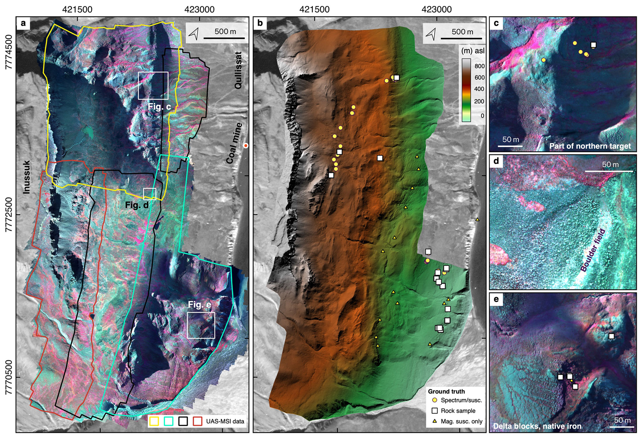
Figure 2Primary data of the multispectral UAS-based surveys after basic processing. (a) Multispectral mosaic at ∼ 20 cm GSD in false colour RGB bands 3, 2, 1. The different polygons outline the survey areas of individual flights. (b) DSM at ∼ 36 cm GSD. Locations of collected ground truth data are indicated with symbols. Inset maps enhance view resolution of areas that were ground-sampled during the study, such as (c) an outcrop associated with the northern part of the target magmatic (d), the central boulder field (e) and outcropping slid volcanic rocks in the southern part.
2.3 Ground-based and laboratory measurements
We conducted ground-based measurements such as magnetic surveys, susceptibility and spectroscopy measurements for validation. In addition, magnetic and electric properties were measured on drill core FP94-4-5 samples, together with a qualitative mineralogic analysis using scanning electron microscopy (SEM). Those measurements are intended to constrain the MVI modelling.
2.4 Ground magnetic surveys
Ground-based magnetic measurements were done at two different areas at Qullissat (survey 4B and 4C in Fig. 3d) with a GEM Systems GSM-19 Overhauser magnetometer at a resolution of 0.01 nT. Measurements of the total magnetic field were made with a mean inline sampling of 1.12 and 1.49 m and line spacings of 50 and 100 m, for the northern and southern survey, respectively. Time and positions were obtained by an integrated GPS receiver and were internally stored together with the magnetic data. A standard data processing for ground-based magnetic measurements was performed with Geosoft Oasis Montaj from Seequent. Diurnal variations in the total magnetic field were removed from all ground magnetic measurements using data from an observatory at Qeqertarsuaq (Godhavn station, identifier: GDH), located at a distance of ∼ 90 km at southern Disko Island.
2.5 Magnetic susceptibility measurements, handheld spectroscopy and grab sampling
We collected representative grab samples and conducted magnetic susceptibility as well as handheld spectroscopic measurements exclusively on basaltic rocks at Qullissat. Magnetic susceptibilities were measured with a KT-10v2 magnetic susceptibility meter. For the majority of locations, we used the average of 3–5 measurements.
Ground spectra were recorded in the VNIR–SWIR range (400–2500 nm) featuring a spectral resolution of 3.5 nm (1.5 nm sampling interval) in VNIR and 7 nm (2.5 nm sampling interval) in the SWIR. Radiance values were converted to reflectance using a pre-calibrated PTFE panel (Zenith polymer) with >99 % reflectance in the VNIR and >95 % in the SWIR range. Each spectral record consists of 10 consecutive measurements. We performed a recalibration after 20–50 scans each, to account for instrument drift. Around 3–5 measurements per GPS point were taken. The main areas covered with susceptibility and spectroscopy are the northern part of the magmatic body, a flat-lying outcrop near the shoreline sediments and at selected spots near a river delta in the south of the investigation area (Fig. 1c, d).
2.6 Petrophysical and scanning electron microscope measurements on core samples from drill core FP94-4-5
The core from the legacy drillhole FP94-4-5 (location in Fig. 3c) is stored in the drill core archive of GEUS (Geological Survey of Denmark and Greenland) and was accessible for this study. We selected core samples in ∼ 10 m intervals in a range from 49.5–215.7 m downhole depth, which comprised samples from both the magmatic body and the sediments above and below it. On these 19 samples, a variety of petrophysical properties were measured at the petrophysical lab of GTK (Geological Survey of Finland) in Espoo. These measurements include magnetic properties such as the induced and natural remanent magnetization (NRM) as well as the inclination and declination of the remanence, electric properties (not shown here) such as the resistivity and the chargeability (both in time and frequency domain), and the dry bulk density. Samples had a diameter of ∼ 3.5 cm and lengths between ∼ 5–10 cm. Susceptibility and NRM is measured with an AC susceptibility bridge (Puranen and Puranen, 1977) and a fluxgate magnetometer (Airo and Säävuori, 2013), respectively. Petrophysical measurements were complemented with detailed mineralogical SEM analyses to link physical characteristics with specific components such as native iron, pyrrhotite, graphite and magnetite.

Figure 3Overview of legacy airborne geophysical (time-domain electromagnetic (TDEM) and magnetic), ground-based magnetic and UAS-based magnetic data with the dashed line highlighting the UAS-based magnetic survey area of this study. The residual magnetic anomalies are shown (a) from the regional AEROMAG97 survey (Thorning and Stemp, 1998), (b, c) from the local exploration airborne survey (Olshefsky and Jerome, 1993) and (d) from ground-based surveys, conducted by Falconbridge Ltd. (grid 4A; Olshefsky and Jerome, 1994) and collected during our field campaign (grid 4B and 4C). The UAS-based magnetic anomaly map is shown in (e) for comparison. The decay constant determined from the electromagnetic data is shown in (b). Two conductivity anomalies were identified (white dots) and considered as targets for further exploration (Olshefsky and Jerome, 1993). The flight trajectories are shown as black lines, and positions of legacy drillholes are indicated in (c) as stars.
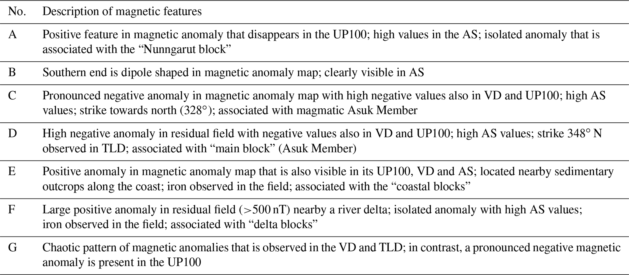
Table 1Magnetic features identified in the residual magnetic anomaly (Fig. 3e) and its associated derivates (Fig. 4).
3.1 Magnetic analysis
Aeromagnetic data are considered as crucial to improve understanding of exploration targets (e.g. Ni-Cu-PGE) in terms of size and depth, and, under favourable circumstances, even age if advanced petrophysical measurements such as thermal demagnetization are conducted (Austin and Crawford, 2019). The main characteristics of our observed anomalies, detected by UAS-based magnetics, are summarized in Table 1 and briefly described below.
Most of the magnetic anomalies are located in the western and central part of the study area at elevation >200 m a.s.l. They are arranged in a complex pattern and have varying strike directions (Fig. 3e). Many of these anomalies have short wavelengths and have both distinct high and low amplitudes in the local residual magnetic field (−400 to −50 nT; Fig. 3e) and in its VD (−17 to −5 nT m−1; Fig. 4b). Since the AS shows high values for both the high- and low-value anomalies (Fig. 4c), it indicates that sharp gradients between magnetic highs and lows exist (Nabighian, 1972; Roest et al., 1992).
Two major short wavelength anomalies (A and B in Fig. 4) are located in the eastern part of the survey area. The positive anomaly A is located directly at the shoreline in the central part of the survey area close to the old coal mine. The positive anomaly B, located close to the Qullissat village, is elongated and strikes NW–SE. At its south-eastern end a dipole-shaped anomaly is present.
In the northern and southern part, short wavelength anomalies (anomalies C and D) show elongated shape (see Figs. 3e and 4b, c, d). The anomaly C in the northern part is oriented in NW–SE (strike ∼ 325∘), but the direction of the southern anomaly pattern D, which consists of a negative anomaly that is margined by a positive anomaly at both sides, is oriented more towards N–S (strike direction ∼ 355∘). In the central area, the anomalies are randomly distributed, and a preferential strike direction is not observed (see pattern G in Fig. 3e and Figs. 4b, c, and in a larger area as chaotic patterns in the TLD in Fig. 4d). Several of these features (C, D, E, F and G) are also observed in the ground magnetic surveys (Fig. 3d), which confirms the reliability of anomalies identified from the UAS-based magnetic data.
These short wavelength anomalies disappear in the upward-continued version (UP100) of the residual magnetic anomaly (Fig. 4a). Instead, negative anomalies become more pronounced in the central western part (see anomalies C, D and G in Fig. 4a), while further to the north and south, the anomalies tend to be positive in the UP100 (see anomalies E and F in the south; Fig. 4a).
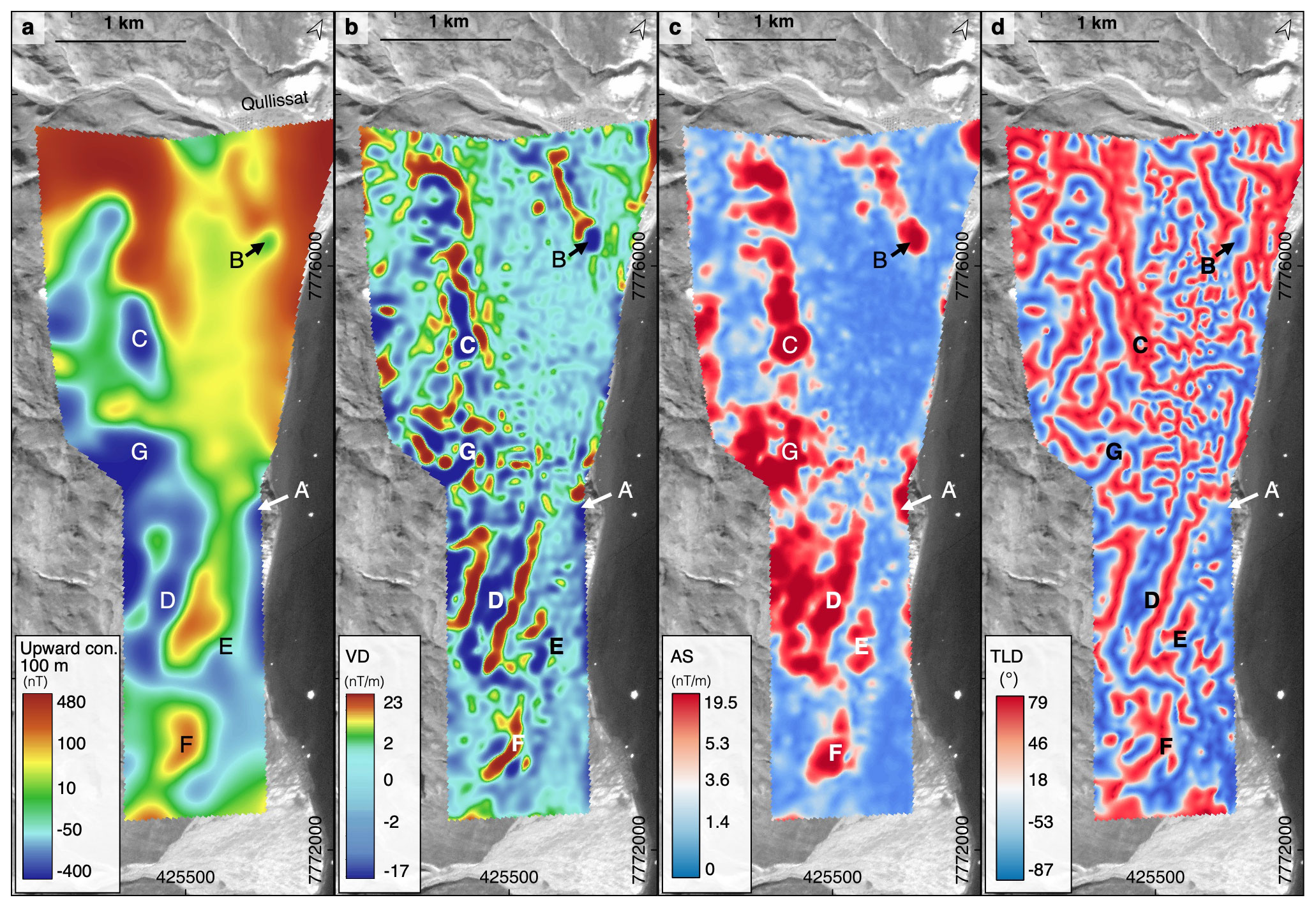
Figure 4Magnetic filter maps obtained from the residual magnetic anomaly of the UAS-based magnetic data in the Qullissat area. (a) The residual magnetic anomaly is upward-continued (upward con.) to 100 m (UP100) to enhance anomalies at larger depths. (b) The first vertical derivative (VD) is presented to enhance short-wavelength near-surface features. (c) The analytic signal (AS) amplitude is presented to highlight areas with increased magnetization, independent of the magnetization direction. (d) The tilt derivative (TLD) map highlights both surficial and deeper structural trends.
3.2 3D magnetic modelling
A 3D magnetization model of the Qullissat area was developed from the fixed-wing UAS-based magnetic data using a deterministic MVI. Employing such magnetic inversion that accounts for the full magnetization vector became more common recently (Ellis et al., 2012; MacLeod and Ellis, 2013, 2016; Liu et al., 2017; Li et al., 2021) and has been applied for example in the mapping of complex volcanic domains (Miller et al., 2020). UAS-based magnetics with close flight line spacing and low ground clearance are especially suited to measuring magnetic remanence (Dering et al., 2019), and experiments confirm that they are reasonably sensitive (Cunningham et al., 2018) to remanent contributions of magnetizations (Calou and Munschy, 2020).
We have chosen an MVI approach because drillhole measurements show that the remanent component of the magnetization partly dominates the investigated magmatic body (see section petrophysical properties). Under such circumstances scalar magnetic inversion only considering the induced magnetization component would likely generate misleading results. However, MVI suffers from a higher non-uniqueness such that additional information (e.g. core logs), measured petrophysical properties, surface structures and different lithologies need to be incorporated to produce geologically plausible models that are consistent with other geoscience data and observations. Therefore, geologically relevant information was added stepwise as constraints during the inversion process.
We have used the VOXI inversion tool in the cloud environment of Geosoft Oasis Montaj (Seequent Ltd., Toronto, Canada). The general inversion setup as described in Ellis et al. (2012) is as follows:
with ϕ being the objective function to be minimized, = (m1,1, …, m1,N, m2,1, …, m2,N, m3,1, …, m3,N) being the model vector containing the three components of the magnetization of all voxels , d being the observed data vector of total magnetic field anomaly at each measuring point and e being their associated data errors. The resulting magnetizations are given in susceptibility equivalences and have SI units. After the targeted error-weighted data misfit was reached in an inversion, the data term ϕD and regularization term ϕM were balanced in the objective function relative to each other such that the solution with the highest regularization was found (i.e. the largest regularization parameter λ was selected, where the targeted chi-squared data misfit was reached; for details see Ellis et al. (2012).
In all inversion tests, a smoothing constraint associated with ϕM,Smooth was added as regularization, and an iterative reweighting inversion focus (Portniaguine and Zhdanov, 2002) option, sharpening anomalies in the model, was active. The smoothing term had, in all inversion tests, weights of 1 in all directions y and for all components p. In addition, the inversion was constrained towards a reference model m0 associated with the term ϕM,Ref for some of the inversion runs. A volume-integrated depth-weighting scheme (Zhdanov, 2002) was applied to ensure that sensitivities are balanced out with depths to avoid that the resulting anomalies are not pushed upward towards the surface.
The main part of the 3D model covered by magnetic data from the UAS survey was discretized in 200 × 267 × 71 cells in x, y and z directions surrounded by a background model with stepwise increasing cell sizes. In the main part, cell sizes in x and y directions were 20 m, whereas cell sizes in the z direction increased with depths from 10 m at 425 m a.s.l. down to 108 m size at −1094 m a.s.l. As the surface topography, we used the regional digital surface model.
The ELM-processed UAS total magnetic anomaly data at a constant altitude of 40 m were used as input data d. An error of 5 nT was assumed for all data points and accounts for inaccuracies in the instrumentation and positioning as well as for high-frequency component loss during the ELM processing.
In the inversion test, no geological information was used in constraints (i.e. no term ϕM,Ref was added). The target misfit (error-weighted RMS data misfit ) was reached after a few iterations, which was also the case for all follow-up runs. However, the first unconstrained run resulted in a geologically unrealistic model (not presented here), where strong magnetic anomalies were partly located in areas associated with the non-magnetic sediments both below and above the magmatic body.
In the following, the different geological units and their magnetic properties were considered in the inversion by establishing constraints of the type ϕM,Ref. For this, the shape of the tabular magmatic body and the location of the basalts along the Inussuk cliff face were estimated. The upper surface of the magmatic body was constructed by interpolation of drillhole intersections of the five Falconbridge drillholes (FP93-4-1 to FP94-4-5), and from outcrop exposures observed in multispectral data (ratios and topography) and RGB images. The top of the outcrops exposures were extracted from the UAS-based DEM (Figs. 5a, 2b). Only the deepest drillhole FP94-4-5 intersected the base of the magmatic body (Olshefsky et al., 1995). To estimate the base, we considered the difference of the top (263 m a.s.l.) and base (131 m a.s.l.) of the magmatic body in this drillhole as the general thickness (132 m) and downward-shifted the top surface with this value. Afterwards, this base surface estimate was compared with the mapped geology along the surface. At locations where the base surface intersects outcropping sediments and basalt, it was modified by shifting it upward and downward, respectively (Fig. 5a). The foot of the basalt cliff (Maligât Formation) was partly covered by debris, but at outcropping sections the surface was observed as being approximately horizontal. Therefore, the associated upper boundary surface of the model environment was considered as a flat and quasi-horizontal plane at 400 m a.s.l. (Fig. 5a).
After adding the magmatic units into the model (Fig. 5b), the remaining part of the model is assumed to be associated with non-magnetic sedimentary units, which is in agreement with field observations. To consider this information in the MVI, we set up a reference model with zero magnetization for all voxels and in all three directions (m0=0). For the voxels associated with non-magnetic sedimentary rocks, the corresponding parameter weights were set to 0.5 for but for voxels containing the magmatic units, the weights were all set to 0.0 ensuring that only the sediment areas were constrained towards small magnetic values.
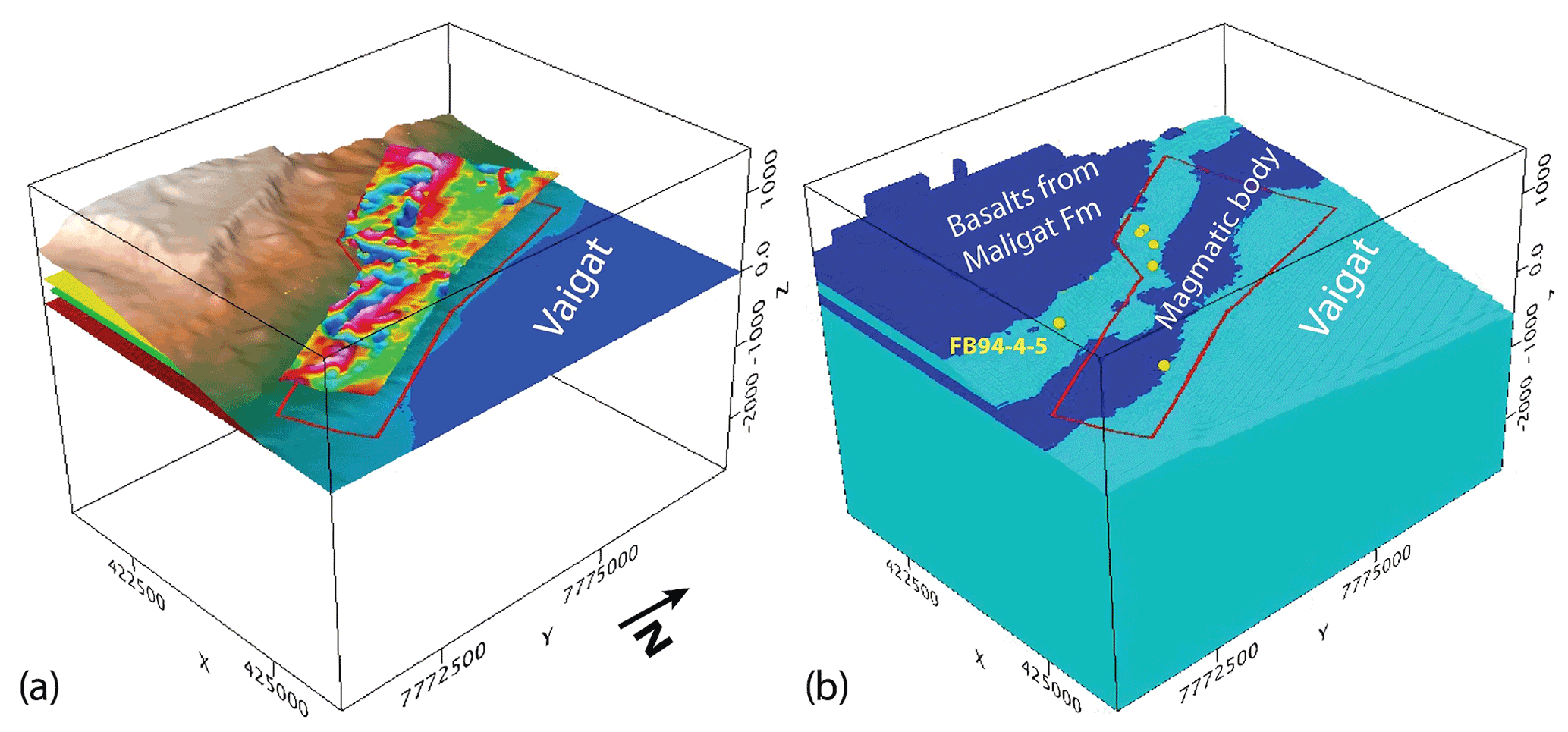
Figure 53D voxel-based model for the magnetic inversion. (a) Topography from the regional DEM is shown together with layers associated with the base of the basalts of the cliff (yellow), and with the top (green) and base (red) of the magmatic body. In addition, the map of the total magnetic field from the fixed-wing UAS survey is presented, whose data were used as input in the inversion. (b) Discretized model used in the inversion. Cells associated with the magmatic body and the basalts from the cliff wall (both in dark blue colours) were derived from the layers presented in (a) and were differently constrained in the inversion as the remaining model (see description of the constraints in the inversion). Yellow dots indicate the locations of the drillholes and the red polygon outlines the area covered by the fixed-wing UAS survey.
Inversion results are presented in Figs. 6 and 7. Only the central part of the model is displayed that is covered by UAS-based data, since the remaining areas are less well-resolved. Higher magnetization values >0.01 SI are almost solely placed in areas defined as the magmatic units and particularly in the mineralized body. The absolute values of the magnetization are with a few exceptions not larger than 0.1 SI (maximum value: ∼ 0.158 SI). In the eastern part, there are only two minor anomalies, which are not located within these units and marked with A and B (Fig. 6b), and no higher magnetizations are assigned to depths below the magmatic body. Within the body the resulting distribution of the magnetization direction is complex and, dependent on the anomaly, high magnetization values are observed for all three components in x, y and z directions. The z component of the magnetization shows both positive and negative values for different anomalies within the magmatic body (Fig. 6b, c, d).
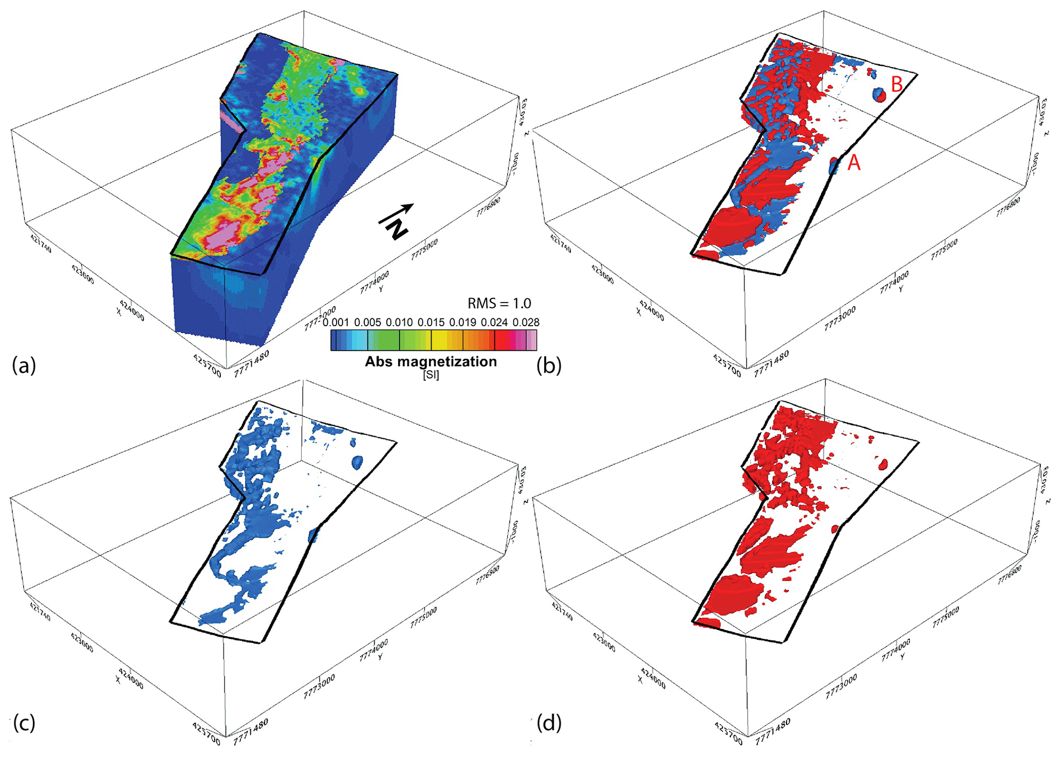
Figure 6Results from the MVI test, where cells associated with sediment units were constrained towards a non-magnetic reference model, while cells associated with magmatic rocks remained unconstrained. Only the shallow central part of the model down to a depth of 1000 m is shown which was covered by data from the fixed wing survey (black polygon). (a) The final magnetization distribution is presented as absolute values of the magnetization vectors. (b) Only cells with absolute magnetization values >0.01 SI are shown as iso-surfaces. Blue and red colours are associated with locations where the z component of the magnetization points out of the ground (z component is positive) and into the ground (negative z component), respectively. These two contributions are presented separately in (c) and (d).
Despite the complexity, the shapes of many of the anomalies show a preferred orientation in a N–S to NNW–SSE direction (see Fig. 7d–i). In contrast, the shape of features A and B located outside of the magmatic units remain rather similar with depth.
Finally, the impact of the magnetic field direction in the inversion was also considered. It was assumed that the Earth's magnetic field and the palaeomagnetic field at the formation of the Asuk Member were oriented antiparallel and constrained by the direction of the ongoing magnetic field (i.e. parallel if the induced part of magnetization dominates and antiparallel if the remanent part dominates). Our assumptions, model constraints and the resulting inversion model are summarized in Appendix C. The resulting model shows some artefacts of small-scaled anomalies (Figs. C1 and C2 in Appendix C).
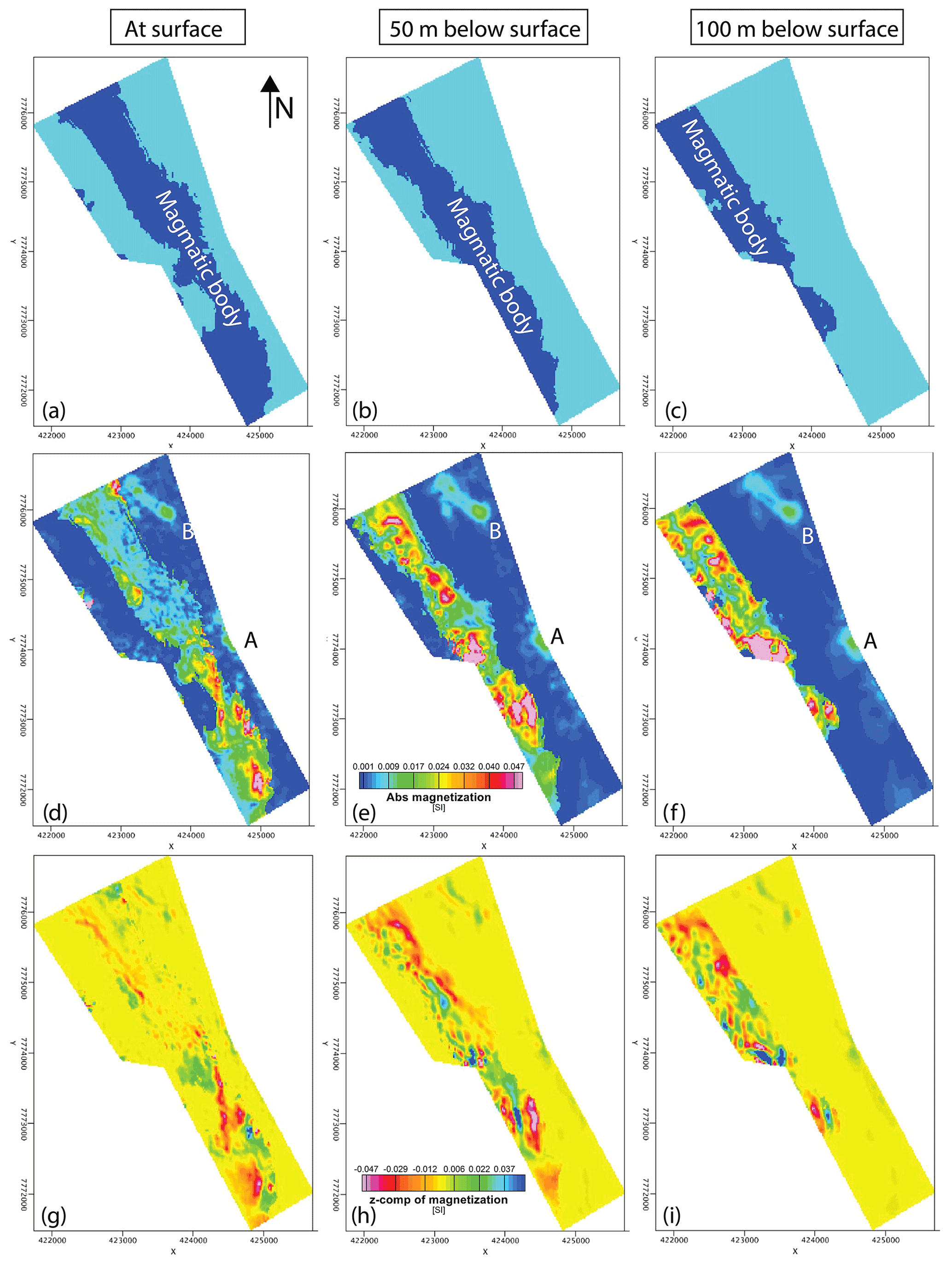
Figure 7Three depth slices through the resulting inversion model, where cells associated with sediment units were constrained towards a non-magnetic reference model, while cells associated with magmatic rocks remained unconstrained. Results are considered at the surface (first column), and 50 m (second column) and 100 m (third column) below the surface topography. In (a) to (c) the reference model is shown, where parts associated with target magmatic rocks are shown in dark blue colours. In (d) to (f) and (g) to (i), the absolute value and the z components of the magnetization are shown, respectively.
3.3 Observations from UAS-multispectral and photogrammetry data
Our multispectral surveys cover the whole region of interest and in addition the cliff of Inussuk with GSDs between 0.18–0.36 m. (Fig. 2). We show the presence of iron-bearing outcrops by means of mineralization proxies for iron alteration minerals and reveal landslide features, e.g. scarps and lobes. The vegetation index (NDVI) mapping (Fig. 8a) illustrates the distribution of widespread low-lying arctic vegetation that covers the surface. NDVI values range between 0–0.71, and we consider pixels with NDVI >0.3 as dominated by vegetation; those are masked out before the image analysis. Vegetation occurs mainly in gently sloping areas and in proximity to water sources, e.g. near stream beds and minor water pathways, all the way up to below the Inussuk plateau. The iron-sensitive band ratio ( ) shows values >1.0 for ∼ 8 % (1.1 km2) for the vegetation-masked orthomosaics. Areas with elevated iron ratios are distributed across the whole study area (Fig. 9). Small blocks and outcrops can be identified by elevated iron band ratios. Large clusters have surface areas of 40 000–90 000 m2 and are located below the boulder field.
The high-resolution UAS-based DSM (Fig. 2b), a hillshade (not shown), the slope (total gradient; Fig. 8b) and a TPI map were used to identify landslide-related features within the study area. A prominent headscarp is visible in the DSM over a length of 1.2 km at an altitude level between 320–350 m a.s.l. (Fig. 8d) and is identified by its concave shape in the contour lines. Smaller rockslides and landslide blocks, which are visible in the DSM (Fig. 8d), are dominant in regions at elevations above 200 m and coincide with the general rockslide area (Fig. 1c). Some of the slid blocks showed glacial abrasion during field examination.
The slope of the topography in the Qullissat area generally rises from the shoreline (slope 0–5∘) towards the foot of the cliff (slope 15–40∘), where the area is undulating and affects the UAS-based magnetic flight altitude. Outcrops form numerous terraces and the slope maximizes at the exposed cliffs of Inussuk (slope >75∘). Most outcrops identified near the coastline (<250 m a.s.l.) have lobate forms, appear strongly disintegrated and are oriented approximately parallel to the shoreline. This trend is observed in the iron band ratio map, where clusters with higher ratios are often arranged in stripes parallel to the shore. The largest outcrop has a size of ∼ 500 × 200 m (150–220 m a.s.l.), and its location coincides with the negative values of the magnetic anomaly D (Figs. 4a, 8d “main block”).
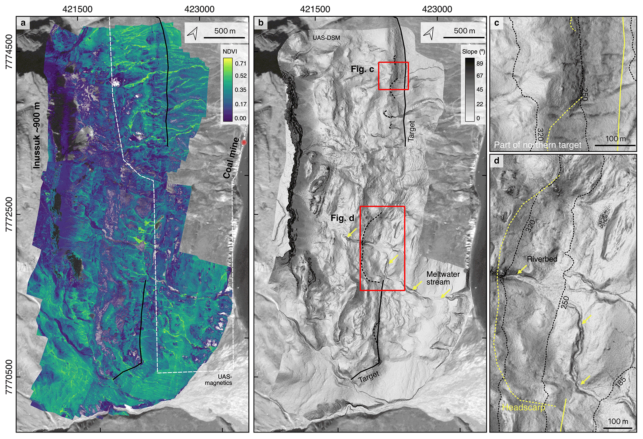
Figure 8Images derived from the UAS multispectral and photogrammetry data. (a) NDVI mosaic derived from the Sequoia camera scenes depicts vegetation occurrence. (b) Slope map (in degree) illustrates the amplitude of the topographic gradient. Inset maps show (c) close-up of the northern part from the targeted magmatic (sampled) and (d) detached blocks with the interpreted headscarp boundary, and a deeply incised meltwater stream.
3.4 Ground-based spectroscopy and magnetic susceptibility
The characteristic iron-absorption feature between 850–930 nm (Hunt and Ashley, 1979; Crowley et al., 2003) is pronounced in spectra of most observed magmatic rock samples (Fig. 9). At the same outcrops, we observed small staining of orange–yellow and reddish- to black-shaded alteration minerals, for example goethite–hematite, yellow–orange jarosite or limonite along outcrops (Fig. 9a). A colour transition from blackish–lustrous to red on some outcrop surfaces is expressed by a change in the surface spectral response. Streak tests on samples from these locations showed a reddish-brown to dark-ochre colour, and their spectra showed a slight absorption band shift from 663 towards 671 nm.
Spectral features of other mineral types were not observed on the surfaces of magmatic rocks, but an abundance of lichen-related absorptions is visible in most spectra as absorption patterns in the short-wave infrared region between 1730–2100 nm. These patterns are often caused by the hydroxyl group and can be characteristic for the presence of lichen, which are abundant in arctic environments (Salehi et al., 2017).
We measured magnetic susceptibility exclusively on magmatic rocks. The susceptibilities are relatively high in the study area (mean value of 0.025 SI and maximum value of ∼ 0.01 SI, Fig. 10a) and are within the range of around 10−3 to 0.01 SI, typically observed for basalts (Clark and Emerson, 1991). There is no major trend of magnetic susceptibility values with their sampling locations (see Fig. 10b, c), although higher surface values >0.03 SI were only measured on less weathered rock surfaces from the basaltic outcrops in the south-eastern and northern parts, which are mapped as in situ outcrops of the target magmatic body (Pedersen et al., 2017). Measurements on rocks with iron-stained alterations, and on rocks located above the target magmatic body (Fig. 10c, presumably Maligât Formation) all had susceptibility values <0.03 SI.
An area investigated in more detail with ground spectroscopy and susceptibility measurements is an outcrop near the coast (Fig. 9a and the close-up in Figs. 12e, 14e), named “coastal block” in the following. It is located at 100 m a.s.l. 300 m east of the main landslide block. Its surface spectra show a pronounced Fe3+ absorption (Fig. 9a) and a magnetic susceptibility range from 0.03–0.07 (Fig. 10a). This outcrop coincides with the positive magnetic anomaly E in the UAS-borne magnetic data, and high iron ratios indicate iron abundance here (Fig. 12b, e).
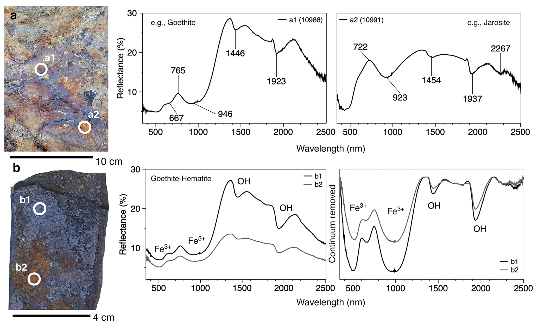
Figure 9Spectral measurements taken on a basaltic outcrop that correlates with the magnetic anomaly E in Fig. 4, with further remote sensing and magnetic characteristics shown in Fig. 12a, b (see close-up location in Fig. 12e). (a) The rock surface shows iron-staining and absorption patterns typical for iron oxide and iron hydroxide (plotted absorption positions taken from Crowley et al., 2003). (b) Spectra (b1, b2) from a sample (GEUS567321) which was scanned under laboratory conditions. Reflectance spectra (left plot) and continuum removed spectra (right plot) highlight the Fe- and the OH-related absorption features.
3.5 Petrophysical properties from cores of drillhole FP94-4-5
The location of drillhole FP94-4-5 was selected on the basis of conductivity anomalies in airborne EM data (Fig. 3b), a ground-magnetic low and anomalously high gold assays (Olshefsky and Jerome, 1994; Olshefsky et al., 1995). It was the only drilling that intersected the whole magmatic body at Qullissat and was probed for Ni, Cu and sulfides. Since the drill cores were unoriented and the actual dip of the drillhole was not measured but assumed to be vertical down to its maximum depth of 270.5 m (Olshefsky et al., 1995), we consider the measured inclination of the magnetization as rather imprecise. Therefore, the inclination is only used qualitatively and carefully in further interpretation. We mainly focus on the results from the density, susceptibility and remanent magnetization measurements (Fig. 10d).
Core logs show the presence of carbonaceous sediments and sandstones in the upper part of the drillhole (depth down hole: 0–50.2 m), before the magmatic body was intersected. The first metres of the body (depth: 50.2–58.1 m) are described by Olshefsky et al. (1995) as a volcaniclastic breccia, which possibly represents a taxite (∼ 54.80 m), but the remaining part of the body consists of fine-grained mafic rocks (depth: 58.1–190.5 m). Below the body, rocks comprise carbonaceous siltstone, shale and sandstone and several thin coal seams (depth: 190.5–270.5 m).
The magmatic body shows significantly different petrophysical behaviour in its upper (downhole depth <127 m; Fig. 10e) and lower parts (depth >127 m; Fig. 10d; 127 m downhole depth corresponds to 190 m a.s.l.; asterisk marks the contact of the two parts). In the upper part, the densities are systematically higher (2774–2803 kg m−3), but magnetic susceptibilities (0.001–0.04 SI), remanent magnetization (0.2–2.4 A m−1) and the Königsberger ratio Q (0.1–0.7) are smaller than in the lower part (densities: 2761–2774 kg m−3, susceptibility: 0.08–0.12 SI, magnetization: 5–15 A m−1, Q: 1.4–2.7). The change in the petrological parameters is abrupt at the transition (or contact), and a single sample at this depth shows reduced densities (2725 kg m−3). However, no obvious change in texture and composition was observed during visual inspection.
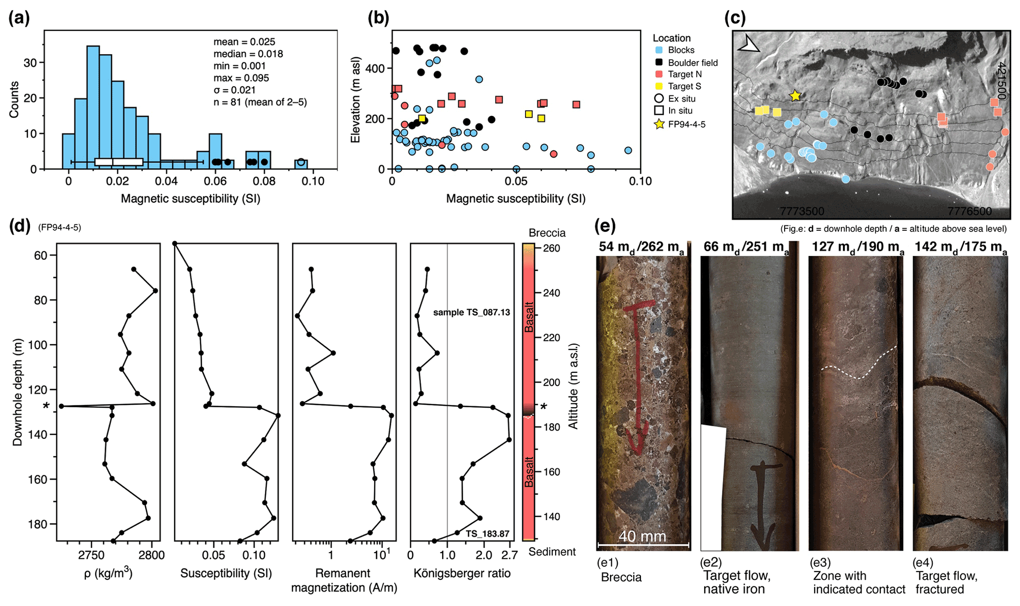
Figure 10Ground-based susceptibility measurements and petrophysical logs from the drillhole FP94-4-5, based on our measurements. (a) Magnetic susceptibility distribution from handheld measurements. (b) Magnetic susceptibility is plotted against altitude (m a.s.l.) with a location-based colour scheme. The locations are given in map (c). (d) Petrophysical measurements of density, magnetic susceptibility, remanent magnetization and computed Königsberger ratio for 19 core samples from the drillhole FP94-4-5. Geologic description taken from Olshefsky et al. (1995), altitude in m a.s.l. given for comparison. The asterisk marks the contact between the upper and lower part of the magmatic body, having different petrophysical properties. (e) Photographs of four representative core sections (md= downhole depth; ma= height in m a.s.l.). We use the reported legacy coordinates but our DEM-based drillhole elevation.
Our mineralogical re-investigations of the legacy cores show that the fine to medium crystalline basaltic flows above and below the contact consist predominantly of plagioclase, orthopyroxene, minor clinopyroxene, and very minor reliclike olivine with an insertal matrix of K-bearing and Fe-bearing glass phases. Native iron is predominantly preserved in the upper block (Fig. 11a, c–e), whereas magnetite and Cu sulfides, such as chalcopyrite and cubanite, are more enriched in the lower block (Fig. 11b, f–h). Nickel-iron phosphides, including schreibersite and pyrrhotite, are present in both blocks with moderately higher quantities in the upper block. Graphite is present in the upper and lower block without any significant difference. Native iron occurs as larger sub-rounded to irregular shaped blebs mostly within tens of micrometres but up to a few hundred micrometres in size in the upper block. Native iron commonly shows a rim of magnetite and/or a low-density Fe-oxide alteration phase (Fig. 11d). Frequently, a “cleaner”-appearing secondary native Fe phase is forming a thin rim around the Fe-oxide phase. Furthermore, native Fe is present as micrometre-sized droplets within the matrix and pheno- and xenocrysts. Pyrrhotite commonly coats the native Fe and Fe-oxide phases and is often associated with graphite. Pentlandite flames and chalcopyrite (and minor cubanite) occur within pyrrhotite (Fig. 11f). In the upper block, the amorphous-phase hisingerite coats the graphite flakes (Fig. 11d). Ni–Fe phosphides occur in schreibersite composition, but also in more Ni-rich undefined Ni–P phases (Fig. 11d, f). The higher occurrences of magnetite in the lower flow correlates with high magnetic susceptibilities and remanence in the petrophysical measurements (Fig. 10d).
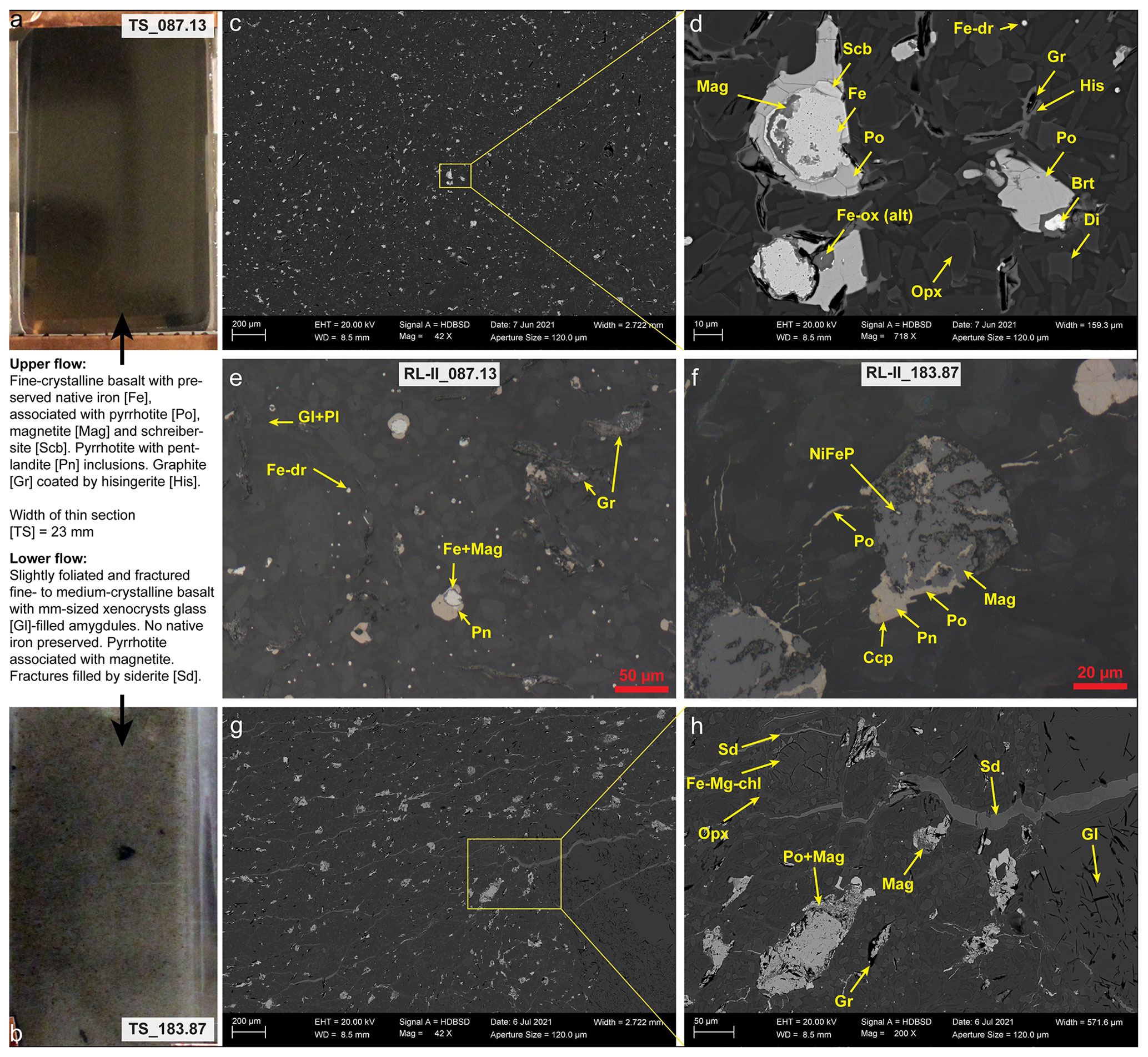
Figure 11(a) Photograph of a polished thin section of a fine crystalline basalt sample from the upper flow (87.13 m core depth). (b) Photograph of a polished thin section of a fine to medium crystalline basalt sample from the lower flow (183.87 m core depth). (c–d) Backscatter electron micrographs (BSE) of sample at 87.13 m depth with preserved native iron (Fe) blebs and Fe droplets (Fe-dr) and minor magnetite (Mag) and Fe oxide (Fe-ox) in association with pyrrhotite (Po), schreibersite (Scb), graphite (Gr) and hisingerite (His). Brt: barite, Di: diopside, Opx: orthopyroxene. (e) Reflected light micrograph of the same sample with larger native Fe blebs with a magnetite rim and association with pyrrhotite and smaller micrometre-sized Fe droplets dispersed in matrix. (f) Reflected light micrograph of sample at 183.87 m core depth with no preserved native Fe, but magnetite in association with pyrrhotite. Pyrrhotite with pentlandite (Pn) flames and chalcopyrite inclusions. (g–h) Backscatter electron micrographs (BSE) of the same sample with pyrrhotite in association with magnetite and graphite and siderite-filled (Sd-filled) fractures that also cross-cut a glass-filled (Gl-filled) amygdule. Fe–Mg–chl: Fe–Mg–chlorite.
The integration of UAS-based high-resolution magnetic, spectral and photogrammetric data (Fig. 12) allows a more detailed interpretation of the targeted magmatic body than previously possible. Magnetic anomaly maps and derivatives together with the constrained MVI model enable us to extend the information into the subsurface to propose a reasonable estimate of the extent and shape of the body. Further interpretation is presented in 3D (Fig. 13).
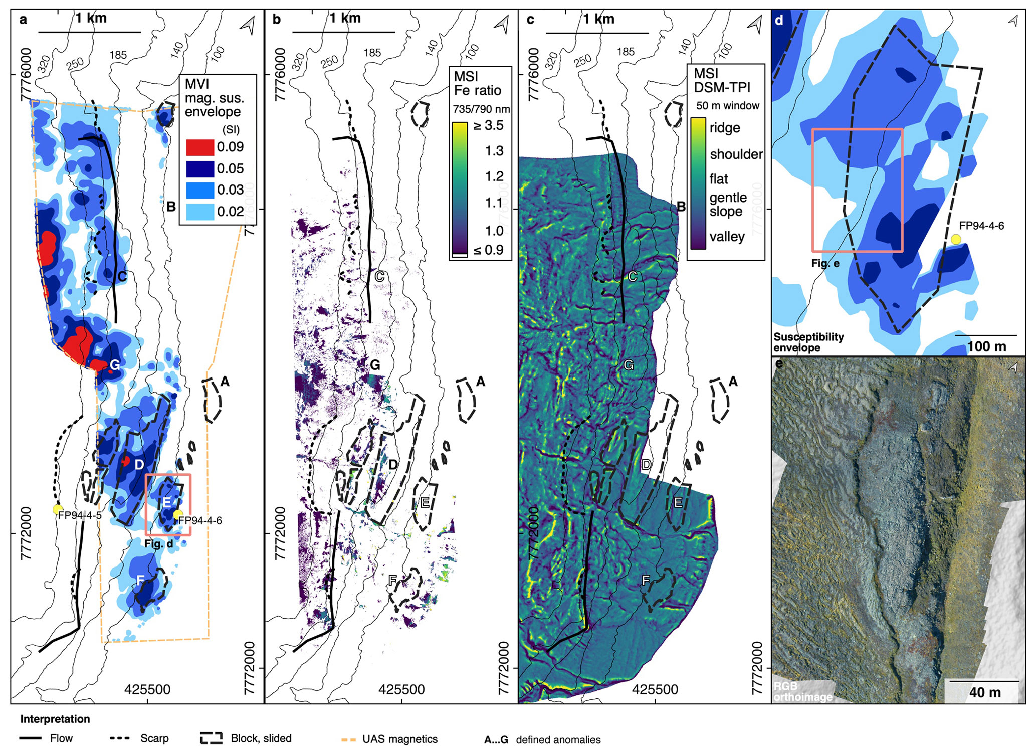
Figure 12Integration of UAS-based data. (a) Isosurfaces of magnetization amplitudes obtained from the constrained MVI inversion. (b) Iron band ratio from multispectral UAS mosaics showing abundance of iron-rich alteration products on the surface. (c) Photogrammetry-based TPI calculated from pixels in a 50 m × 50 m moving window shows graduation from incised valleys, to flat slopes, to ridges. (d) Isosurfaces of magnetization amplitudes from the MVI model. (e) RGB orthomosaic from a single RGB reconnaissance flight (DJI Mavic). The letters A to G refer to the magnetic anomalies defined in Fig. 4.
4.1 Location, shape and size of the mineralized body
Based on the distributions of (1) outcrops of magmatic rocks identified from the DSM and (2) distinct magnetic anomalies (Figs. 3e and 4a–c), we propose that the targeted magmatic unit is located between ∼ 140–320 m a.s.l. (Fig. 12). However, due to landslide activities in the central and southern part of the survey area, ∼ 3 km south of Qullissat, several detached blocks slid down and we identified ex situ basalt blocks down to the sea level (Figs. 12, 13, 14). We estimated the surface exposure of the main target body to be ∼ 4.5 km2 in the study area based on magnetic anomalies, drillhole and outcrop observations, but detached and sliding blocks from the body cover an area of ∼ 0.50 km2 (Fig. 14b). Since magnetic anomalies are observed at the boundaries of the UAS-based magnetic survey, we assume that the body continues beyond the survey area below the mountain range towards the NW and W. However, it would be difficult to identify the magmatic body by magnetic measurements there, because the magnetization of younger basaltic units (mainly Maligât Formation) at higher elevation obscure the magnetic response of the body. Towards the S and E, the erosion elevation level is lower than in the central area and the magmatic body is eroded.
We interpret the targeted body to be a flat-lying, tabular-shaped body, from information of mapped outcrops in the DSM and from the available drill hole elevation data (Olshefsky and Jerome, 1994; Olshefsky et al., 1995). This constraining information is in agreement with the results from the 3D magnetic inversion, because almost all magnetic anomalies can be modelled with a body that has magnetic properties within a reasonable data range (susceptibility equivalents of 0.1–0.15 SI). However, the limited resolution of the magnetic method and uncertainties in the surface used for the base of the magmatic body, which is determined only from information along outcrops and a single drillhole, do not allow us to reliably interpret further details of shape and thickness variation (Blakely, 1995).
The top and base surfaces were partly determined from outcrop information in the DSM. These outcrops are not only from the main target body, but also from the slightly displaced “main block” (Sect. 4.2). Therefore, the magmatic unit in the inversion model does include partly unstable rock mass. However, these displacements in the height direction are only minor (<50 m) and have little impact on the overall surface shapes.
The appearance of pronounced long-wavelength negative magnetic anomalies in the upward-continued version of the residual anomaly (see anomalies D and G in Fig. 4a) can be explained by magnetizations with a dominating reverse polarization that are located at considerable depths and, hence, supports that the body has a significant thickness of more than 100 m.
The alternation of high-frequency anomalies in the UAS-magnetic data with strongly varying intensities (i.e. the high analytic signal of feature D; Figs. 4b, c, 13c) supports our understanding that low magnetic values over the body are not created by a lack of magnetic material. More likely, there is a significant remanent magnetization contribution that is oriented in a distinctly different direction than the induced magnetization. This is also supported by the results from the constrained inversion. Because the investigation depth to resolve structures is highly limited for this local, quite narrow magnetic survey, it is hard to evaluate if any major magnetic material, e.g. from intrusions, is located underneath the body. In any case, the 3D inversion results show that an approximately horizontal magmatic body with reasonable magnetization values can explain the full data response, and no deeper-seated structures, e.g. those associated with a feeder structure, need to be added to fit long-wavelength trends.
There are plausible explanations of why the anomalies A and B (Figs. 3, 4, 6, 7) are located outside of the estimated body. Anomaly A, coinciding with the “Nunngarut” block, is located in the central-coastal area that is most affected by mass movements and may be associated with a larger fragment of the body that slid downward (see next section about landslide features). However, anomaly A also coincides with the location of the entrance from the former coal mine shaft, where some metallic mining equipment has been left. Anomaly B is located within the Qullissat village and may be associated with a construction built on a solid rock foundation that is described as native-iron bearing. In the inversion results (Fig. 7d–f), it is observed that the magnetization anomalies of A and B are very much unchanged over a depth range of 100 m. It is likely that these appearances are not representative for the true magnetization distribution but caused by the constraint towards a non-magnetic reference model that enforces small magnetization values in areas that are assigned to sediments in the inversion model. To fit the data responses it is required that the magnetization anomalies of A and B extend over larger depth ranges.
Anomaly C is described as part of the magmatic target unit both in the regional geologic map (Pedersen et al., 2013) and the photogrammetric cross section of the Qullissat area in Pedersen et al. (2017). The other anomalies D, E and F (Fig. 13a, b) are associated with displaced material, the locations of which are only roughly sketched in the cross section (Pedersen et al., 2017). Handheld rock samples from those blocks (e.g. Figs. 9b, 10c, 12e) contained native iron, pyrrhotite and magnetite, observed on thin sections (sample location in Fig. 2c, e). Those samples also showed a similar texture to that seen in the cores of the drill hole FP94-4-5 (Fig. 11).

Figure 13Combined plots of surface topography (PlanetScope mosaic fused with ArcticDEM) and larger magnetization amplitudes (≥ 0.03 SI) in the subsurface from the MVI model: (a) top view of survey area; (b) side view cross section facing north – dashed lines indicate the maximum extension of the intrusive body; (c) oblique view from the east. In all three views the surface model is removed for areas where the magmatic body is present at the surface (compare Figs. 12a, 14a). A possible extension of the target unit is sketched next to the main block, anomaly D.
4.2 Linking landslide features to the exploration target
The curved shape of the head escarpment of the landslide identified in the UAS-DSM proposes a concave rupture surface (Figs. 13 and 14a, b) and following known landslide classification systems (Varnes, 1958; Hungr et al., 2014), we considered it as a rotational rockslide. The material from the landslide is uniformly composed of mafic rocks and consists of one large block (“main block” in Figs. 13b, 14a) and a number of smaller blocks (such as the “delta block”, “coastal block” and “Nunngarut block” in Fig. 14a). Most of the slid material occurs in proximal distance to the head scarp (“main block”) and seems to be moved only slightly, but some larger rotated blocks (e.g. “delta block”, “coastal block”; Fig. 14a, e) were identified at distances of up to ∼ 1 km from the headscarp (interpreted from multispectral maps and DEM data in Figs. 8b, 12c). Several of these blocks were associated in former investigations with parts of the targeted Mg-rich andesite intrusion from the Asuk Member (Pedersen et al., 2017).
The magnetic anomalies A, D and E (Fig. 4), and probably the patterns F and G, are located within areas that are affected by landslide movements, but the anomaly C is located in a presumably stable area (Fig. 14a). The anomaly pattern D is associated with the largest “main block”, and its deviation of the strike directions (strike ∼ 355∘), compared to the general NW–SE arrangement of magnetic anomalies and the strike direction of anomaly C, can be explained by a rotating component (along a virtual z-axis) during the landslide event. Blocks D and E are surrounded by streams, where flows carved into the more brittle rock fragments and buried crevices (Fig. 14a).
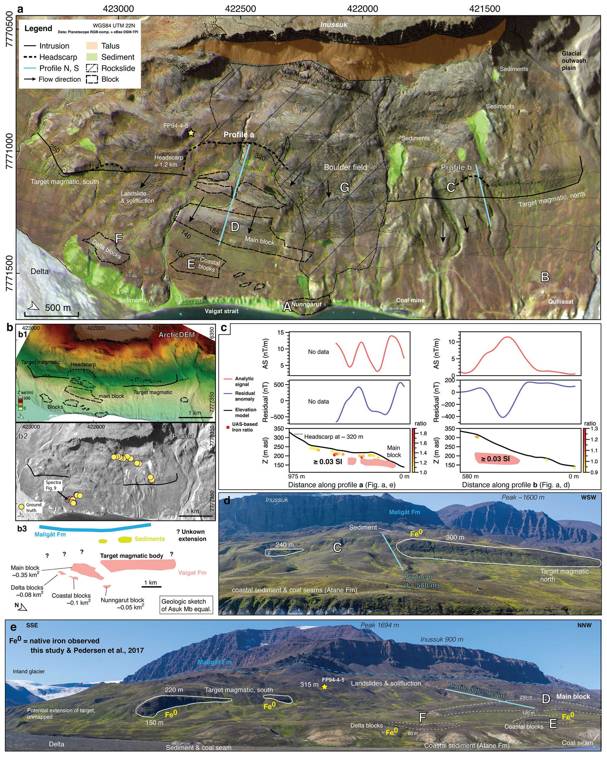
Figure 14Integrated interpretation (a) RGB-composite plot from PlanetScope images (Planet Team, 2017) that are merged with semi-transparent TPI from the eBee DSM to increase image contrast. Landslide features are marked as dashed lines with thin lines for larger blocks and thick lines for the main landslide scarp. Talus below the Inussuk and block fields are the source for numerous boulders in the whole area. Mapped sediments reach up till the foot of the Inussuk cliff. (b) Overview maps illustrate area in relation to the different data: (b1) ArcticDEM at 2 m resolution with interpreted blocks, (b2) PlanetScope greyscale mosaic with ground truth locations (spectroscopy and magnetic susceptibility) and (b3) sketch showing the assumed extent of the target magmatic body (only the part covered with UAS data are shown). (c) Two schematic cross sections in the west–east direction are shown together with the magnetic anomaly and the analytical signal from the UAS-borne magnetic data, and iron ratios extracted from the UAS-borne multi-spectral data. The locations of these cross sections are sketched in (a). (d–e) Coast-side views onto the magmatic outcrops in the (d) northern and (e) southern part of the study area.
The locations of the “coastal block” and “delta block” both coincide with a magnetic anomaly (E and F, Figs. 4 and 14a) indicating that these landslide blocks consist of magmatic rocks with elevated magnetic properties proposing that they also originate from the targeted magmatic body. Samples taken near the slid “delta block” and from the northern part of the intrusion, which is not affected by landslide movements (Figs. 8c, 14a, e), are similar in their geochemical and microscopic compositions (Fig. 11) strengthening this interpretation. Also, the Nunngarut block located immediately at the shoreline and adjacent to the coal mine coincides with a small but distinct positive magnetic anomaly in the residual magnetic anomaly (Figs. 3e and 14a). This is observed in the analytic signal (feature A in Fig. 4c) and results in a spot with elevated magnetizations in the MVI models (feature A in Figs. 6 and 7). Rocks of this block have a similar geochemical composition to the intrusion (Olshefsky and Jerome, 1994), the sample AF0903 from the Nunngarut block (Olshefsky and Jerome, 1993) and the GEUS sample 156 690 (Pedersen et al., 2017), which is taken from the southern part of the targeted magmatic body. Those samples show similar contents of Mg (6.5 %–7.6 %) and Fe (10 %–12 %) (Pedersen et al., 2017). The chaotic anomaly pattern G in the central-upper part of the survey area may indicate disrupted rocks from landslide movements (Figs. 4 and 14a). However, this area is covered with breccia and hyaloclastites, as well as talus material from the cliffs, and the magnetic response can also be explained by other deposition processes.
4.3 Distribution of iron alteration products
UAS-based multispectral iron ratios provide information on the distribution of iron-bearing minerals as a proxy for mineralization. We anticipated that the use of these data for interpretation is limited because spectral identification of surficial iron occurrence relies on one band ratio combining two bands with broad spectral ranges and low sensitivities. In addition, the ratios were affected by cast shadows in multispectral images, and band 4 (790 nm) has a higher uncertainty due to low reflectance of volcanic rocks. Therefore, the ratios can be systematically biased, and in particular multispectral pixels with higher ratios (>3.0) might be misleading. In similar studies, we recommend further examination, if high ratios occur as spatially isolated anomalies. Even after data cleaning, numerous pixels with non-illuminated edges and shaded zones remain in the orthomosaic. Therefore, we re-evaluated selected spectral absorption zones by visual interpretation, by using the UAS-based false-colour orthomosaic (Fig. 2a) and additional RGB imagery from high-resolution satellite images (Team Planet, 2021). This auxiliary information helped to remove obviously false absorption zones, e.g. shadowed sedimentary units.
Iron ratios >1.0 identify outcrops with iron alteration and ratios >2.0 are interpreted as patches that can indicate potentially mineralized blocks and boulders (in total 0.02 km2 or roughly 3 %–5 % of the covered surface). We considered those zones of interest for closer ground inspection (Figs. 2, 12b). Many of the spots with high ratios in the upper western part coincide with areas where material from lava flows and hyaloclastites were emplaced, and they can be associated with basalt blocks and talus material that originate from the iron-bearing Skarvefjeld Unit (Maligât Formation) of the adjacent Inussuk mountain. In the lower central and eastern part, high ratios are likely associated with iron from the magmatic body of the Asuk Member. The largest landslide block (“main block”) is associated with ∼ 50 000 m2 of measurable iron absorption (iron ratio >1.05, Fig. 12b). Also, two other outcrops (“delta block” and “coastal block”) in the southeast of the study area had surfaces with elevated band ratio values. They were closely investigated from the ground, and iron stains were found (Fig. 12b; “coastal block” outcrop is captured by the DJI Mavic RGB images in Fig. 12e). Our handheld spectroscopy indicated a subtle change from iron oxides (hematite) to hydroxides (goethite; specific spectral features; Crowley et al., 2003), a crystal structure change, which is related to a compositional alteration.
4.4 Mineralogical considerations and explanations for magnetic anomalies
The occurrence of goethite (α-FeOOH) and hematite (Fe2O3) is observed as specific absorption features in the surface spectra at five investigated outcrops and is associated with iron-bearing magmatic bodies (Fig. 9). These oxy-hydroxides can be alteration products of both the magnetite and titanomagnetite abundant in the basalt (Pedersen et al., 2017) or the result of corrosion of native iron (Figs. 10, 11). Magnetite, titanomagnetite and native iron are ferrimagnetic (magnetic susceptibility ∼ 1–100 SI for magnetite; estimates for native iron in nature are limited due to its rare occurrence), and all can contribute considerably to the magnetic behaviour in the contaminated magmatic body. Another contributor to the magnetic response could be monoclinic pyrrhotite (Fe1−xS; Clark, 1997; Austin and Crawford, 2019).
First results of our re-investigation of drillcore FP94-4-5 with SEM and petrophysical measurements indicate that the higher magnetic properties (Q, susceptibility, remanence) in the lower part of the drillhole (Fig. 10d) correlate with a higher content of magnetite. In contrast, native iron is present in significant amounts only in the upper part that has lower magnetic properties, which suggests that native iron is not the main source for magnetic characteristics. Since the content of pyrrhotite is in the same range or lower than the content of magnetite, and because the magnetic ferromagnetic magnetic properties are distinctly higher than from pyrrhotite, we concluded that the magnetization from magnetite is more dominating than from pyrrhotite. Moreover, the Königsberger ratios from monoclinic pyrrhotite in rocks are typically very high (Q of tens to hundreds, depending on its domain state; see Fig. 3 in Clark, 1997), but our observed Q values do not exceed 2.7 in the core samples (Fig. 10d). This implies that the magnetic responses are probably not diagnostic for the mineralization in this body, which has major implications for the use of magnetic data for sulfide exploration in this area.
Although native iron is not the main source for the magnetization in the body, it is harder to judge if its contribution is significant in its upper part, in which magnetization is still significant although clearly smaller than in the lower part (Fig. 10d). Nagata et al. (1970), who investigated lunar material, stated that very fine-grained native iron can have a superparamagnetic character. This means that its ferromagnetic remanence can have a major component that changes its orientation in the direction of the outer field (viscous magnetic remanence) at temperatures significantly below its Curie temperature (771 ∘C). If the native iron has such a superparamagnetic character (or has a softer remanent magnetization for other reasons) at Qullissat, much of its viscous component may be turned along the current Earth magnetic field direction resulting in lower Q values. Indeed, we observe lower Q values in the upper part (Q=0.1–0.7) of drillcore FP94-4-5, where native iron is abundant, than in the lower part (Q=1.4–2.7). However, other factors such as grain sizes of magnetite have an impact on the magnetic domains, and finer grains are usually associated with a larger Q ratio (Dunlop and Argyle, 1997).
The abrupt change in all measured petrophysical properties in the drillhole at a depth of 127 m is notable (Fig. 10d). The question arises of whether the change is associated with (1) two separate successive magmatic pulses, which differ in their geochemical and accordingly also petrophysical properties, or (2) segregation processes in the liquid magma during formation. Several observations propose the former explanation as the reason for the abrupt change in mineralogy and magnetic properties at the contact zone. Also the low-density spike (ϱ=2725 kg m−3) at this depth could be explained as a zone of increased weathering by exposure to the ground surface or alteration by heat from a subsequent magmatic event.
If these two units are from separate magmatic events, they could be extrusive lava flows intruding into the soft sediments or covered by material afterwards, and not a sill, as stated in former studies (Olshefsky and Jerome, 1994). Currently, a manuscript from Pedersen et al. is in preparation that will discuss this aspect in detail. Higher values in both induced and remanent magnetization in the lower part of drillhole FP94-4-5 (Fig. 4a) suggest that lower flows of the first pulse are more magnetic than flows of the later pulse. This would explain why distinct anomalies can be found in the upward-continued version of the residual magnetic anomaly (Fig. 4a, anomalies D and G), where stronger magnetizations at larger depths are enhanced. The negative character of these anomalies is in agreement with higher Königsberger ratios in the lower part of the drillhole (Q>1.0) provided that the body was emplaced during a period of magnetic pole reversal. Accordingly, the appearance of such negative anomalies is in accordance with the interpretation from Pedersen et al. (2017) that the body belongs to the Asuk Member.
In the upper part of the drill hole, the Q values are slightly lower than 1.0 such that predominantly slightly positive anomalies are expected at shallow depths, even if the body is formed during a period of phase reversal. This is in agreement with the magnetic survey data, where both positive and negative short-wavelength anomalies are observed indicating that in some areas the induced and other areas the remanent magnetization dominate in the shallow part of the body. In the 3D inversion results such a distinction of two layers having clearly different magnetic properties cannot be observed. In contrast, a rather complex pattern of magnetization varying in both magnitude and direction suggests a more complex distribution of material with magnetic properties (as magnetite, native iron and sulfides). However, since magnetic inversions have a very limited resolution (even if the inversion is constrained), we cannot exclude that the magmatic body consists of two distinct flows with significantly different magnetic properties across its whole extent or in major parts.
Although the remanent magnetization seems to be predominantly oriented into a positive z direction (the Earth's magnetic field has a large component in the downward z direction), inversion results do not necessarily support that its direction is uniform and always parallel to the palaeomagnetic field direction. So, the obtained range in magnetic susceptibility equivalences (from 0.1 up 0.15 SI) in the first constrained inversion run, where only the sediments were considered as non-magnetic, are in the same range of magnetizations as observed in the drillhole FP94-4-5 (Fig. 10d, susceptibilities of 0.12 SI and remanent magnetizations of 15.2 A m−1). However, the values obtained in the second inversion run, where in addition the overall magnetization is assumed to be aligned either parallel or antiparallel to the Earth magnetic field (and palaeomagnetic field), are unreasonably high (up to 0.4–0.6 SI; additional inversion runs in Appendix C) to represent the values from the petrophysical measurements. In addition, alignments of some larger trends in NS to NNS–SSE (Fig. 7d–i) directions, as observed in the first inversion run, appear geologically more reasonable than the artefact patterns with many small-scaled features observed in the second run (Fig. C1). Accordingly, we assume that the results of the second inversion run are less meaningful than those of the previous run, although the target misfit (RMS = 1.0) was reached in the second run, making it a solution theoretically. This means that it is likely that the magnetization direction is a complex distribution and not only aligned along the palaeomagnetic field and the current Earth's magnetic field.
Two aspects could explain varying directions of the magnetic remanence. (1) In the case that native iron measurably contributes to the magnetic behaviour and a major component of its remanence has a viscous magnetic character, this could impact the overall direction of the remanence. It can be imagined that its magnetization direction changes after rock formation and accordingly deviates from the direction of the palaeomagnetic field. (2) Rotational components of the landslide and other mass movements may change remanence directions in a complex manner; particularly in the unstable areas in the south. Because the magmatic body was presumably not impacted by major metamorphism or heating up events after its formation in the Palaeocene (63 Ma), it is quite unlikely that the rocks reached Curie temperatures afterwards. As such, we see thermal demagnetization as an unlikely reason for the complex magnetization directions.
Our results demonstrate that an integrated workflow of UAS-based optical remote sensing and magnetic data with supplemental measurements from the ground and drillholes is advantageous to precisely map and describe a mineralized magmatic body at depth and to improve the targeting of potential Ni–Cu–Co–PGE mineralization. Although the body is mainly hidden at the surface, we obtained significantly more detail than what was possible from all formerly acquired legacy data. Thus, we conclude the following:
A plausible lateral extent of the magmatic body could be proposed from the distribution of the magnetic anomalies and results from a constrained 3D magnetic inversion, where the upper and lower boundaries of the body were estimated from observations in the DSM and drillholes. It allowed us to develop a realistic 3D model of the body that agrees with and augments former interpretations (Pedersen et al., 2017). It proposes that the body has a flat-lying tabular shape and extends across large parts of the south-western survey area. However, more detailed information on the variation of the lower boundary cannot be determined currently, as the surface is derived only from outcrop observations at the slope surface and from a single drillhole, and the magnetic method suffers from an inherently low resolution.
The shapes and arrangement of the shallow magnetic anomalies indicate that larger blocks of the magmatic body were displaced by landslides. By identifying landslide features in the DSM and relating them to detailed magnetic anomaly patterns, it was possible to determine precise locations and extents of these blocks. Because major parts of the body do not outcrop, this would not have been possible from surface observations alone.
The presence of negative long-wavelength magnetic anomalies indicates a significant remanence that proposes a reversed Earth magnetic field during its formation. This is in agreement with interpretation that the magmatic main unit was emplaced during the pole reversal associated with magnetochron C26r and is part of the Asuk Member of the Vaigat Formation (Pedersen et al., 2017). A strong remanent magnetization component is confirmed by the petrophysical measurements from cores of drillhole FB94-4-5 (Königsberger ratio up to 2.7).
An unexpected observation from the MVI results is that the remanent magnetization direction in the body does not seem to be uniformly oriented parallel to the palaeomagnetic field. The reasons for this are not understood yet. Explanations could be potential rotational movements (e.g. from slope instabilities) after the Curie temperature was reached or uncommon magnetic behaviour of native iron.
An abrupt change of the petrophysical measurements in drillhole FB94-4-5 indicates that the magmatic body is split into an upper and lower part with distinctly different physical properties and presumably varying compositions. The most plausible explanation would be two separate magmatic events, i.e. lava flows, which supports a hypothesis that the bodies were formed extrusively. Therefore, a detailed SEM mineralogical study has been initiated, but too few samples were systematically investigated, when this paper was submitted, to draw any quantitative conclusions of compositional variations. A combined quantitative mineralogical and petrophysical analysis at a microscale is advised to clearly identify the minerals responsible for the magnetic anomalies. Native iron, pyrrhotite and magnetite are observed in hand samples and core pieces. At this stage we only conclude that magnetite is generally dominating the magnetization. Thus, our knowledge on the contribution of the magnetic properties caused by pyrrhotite and native iron remains incomplete. In this context, it is in both exploration and academic interests to investigate how native-iron-related magnetization and its resulting anomalies are expressed. Native iron is geologically rare and its magnetic response in field practice is barely investigated.
Experiments to determine magnetic properties with increasing temperature and alternating fields will help in this context, e.g. as illustrated by Austin and Crawford (2019) on Ni–Cu–PGE mineralization in Australia. From such measurements, it is possible to identify rock forming and environmental effects, metamorphic overprinting, and a better geologic understanding of how such magmatic suites form. We postpone these measurements at this stage, since the core orientations are unknown and accordingly much of the obtained directional information would be spurious. Oriented core samples would need to be gathered first.
Because only one drillhole intersects the base of the magmatic body and the magnetic method has a limited resolution, it is highly recommended to incorporate further constraining information to refine the estimate of the magmatic body base. Both new drillholes intersecting the base and integration of other geophysical data by, for example, joint inversion approaches could help in this context. The available airborne GEOTEM data could not be used to improve the estimate of the thickness, but integration of magnetic data with existing MT data and newly acquired airborne EM data using more recently developed instruments should be considered.
A far-reaching goal is a better understanding of sources (native iron, magnetite, graphite and pyrrhotite) that cause the observed anomalies in different types of geophysical data and not exclusively magnetics. This requires incorporating further geophysical information, e.g. electrical properties from samples and results from airborne EM and MT measurements, which might have characteristic responses for graphite, pyrrhotite and presumably native iron. In this context, one of the existing MT profiles in the Qullissat area shows a very pronounced high-conductive anomaly immediately outside the western border of the magnetic UAS survey at a depth that correlates with the bottom of the magmatic body (Blue Jay Mining PLC, personal communication, 2021). There are different hypotheses about the anomaly origin and plans for a new drillhole at this location. Finally, we recommend expanding the use of integrated UAS-based multi-sensor surveying for geologic targeting with more sensors to identify mineral groups and to improve differentiation of iron-bearing minerals.
Flight performance is controlled by a live-link software via telemetry connection. A GSM-based tracker device allows the UAS to be located in case of lost telemetry signal. A magnetic and barometric base station, which is placed near to the mobile telemetry and control station, measures the time-variant part of the magnetic field (three-component fluxgate magnetometer) and the barometric pressure.
In the post-processing of the data, the magnetic field (and optionally the barometric altitude) measured by the moving UAS platform is corrected by the variations measured at the base station. For these surveys, the dedicated base station magnetometer was not available, and a replacement UAS magnetometer was used for the base. The basic data processing (Table A1) utilized the RadaiPros software (version 2.0, Radai Oy, Oulu, Finland). After these general processing steps, (1) data were checked visually and invalid or unnecessary points (e.g. spikes and flights between the home base and the survey area) were removed, (2) base station correction was applied to the magnetic total field data, (3) separate flights were combined and data outside of the survey area were taken out (with 25 m margins), (4) a low-pass filter with a cut-off wavelength of ∼ 20 m was applied, (5) an ELM was conducted, and finally (6) the IGRF core field was removed.
In the ELM method, first a deterministic inversion is used to find a simple susceptibility model, whose synthetic response fits the measured magnetic total field. In a second step, the obtained susceptibility model is used to compute the total magnetic intensity at a constant elevation level on an even grid. Here, the susceptibility model is composed of a single layer of magnetized 3D cells.
The ELM method reduces the effects of varying flight altitude and uneven sampling of the data points, high-frequency noise and artefacts provided that their wavelength is short compared to the size of the elements used in the layer model. ELM is used also to level the datasets and make the heading correction. The ELM was applied to the fully pre-processed total field data. Horizontal size of the elements was 40 m × 40 m and their vertical height was 111 m. Depth to the top of the model was 2 m, and the top of the model followed the terrain topography. The total number of elements was 148×64 = 9472, and the total number of (decimated) data points was 12531 (15.10 %).

Agisoft Metashape (version 1.6, Agisoft, St. Petersburg, Russia) is used to process multispectral data and create digital surface models as raster and 3D point clouds, multispectral orthomosaics from each flight area, and the complete flight area in one image. A total number of 11 eBee MSI flights in four sub-areas were conducted totalling 308 line kilometres. The flight lines were set parallel to the regional slope with terrain following and with a forward and sideward overlap of 80 % and 60 %, respectively.
For spectral calibration, three images with different image acquisition settings (i.e. different integration time to adjust for varying illumination strengths) were taken from a ground reference target (Airnov™ VIS-NIR greyscale panel). These calibration images are automatically detected in Agisoft Metashape or selected manually. Our settings in the image alignment step are alignment accuracy in high, pair selection with reference and adaptive camera model fitting being activated.
After each step, the points were filtered with gradual selection repeatedly, and the option “optimize cameras” was applied each time to reduce alignment errors (see for example the 3D remote sensing lab at SLU Umeå, Sweden, http://www.rslab.se/agisoft-photoscan-pro, last access: 4 March 2021). After the correction steps were applied, the sparse points were used to create a dense point cloud, using the “high quality” settings in the creation dialogue. From the dense cloud, we exported the elevation model, the orthophoto in reflectance and the 3D point cloud (reference standard WGS84 UTM 22N, EPSG 32622).
We assume that the remanent magnetization in the magmatic body has roughly the direction of the palaeomagnetic field, when the body formed, since no tectonic processes with major rotations have taken place after the formation of the basalt. However, this must be considered carefully, since the central part of the investigation area has been affected by slope instabilities and rotational movements might be associated with them.
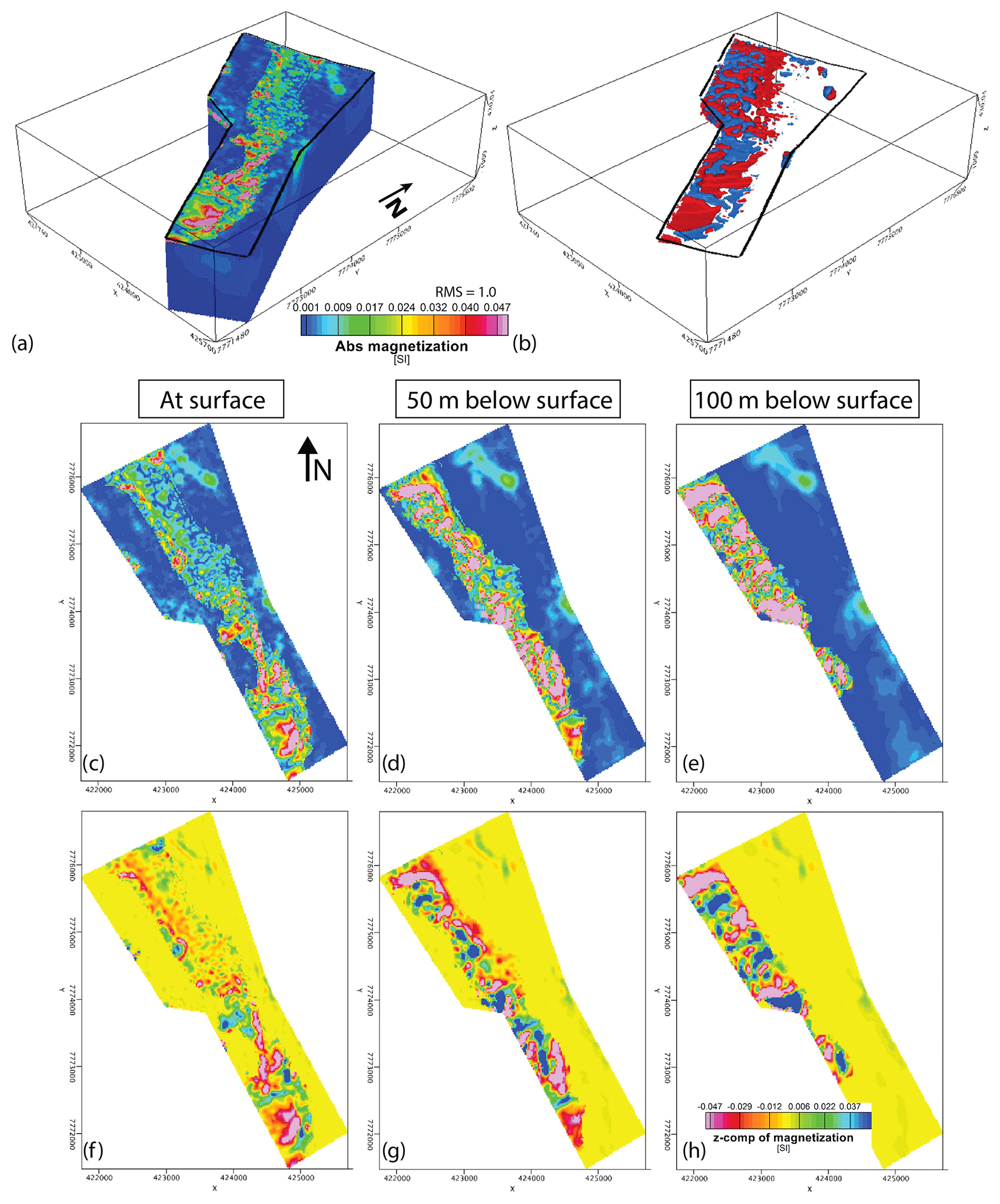
Figure C1Results from the inversion model, where in addition the direction of the magnetization in the magmatic units is constrained towards the direction of the regional magnetic field. (a) The final magnetization distribution is presented as absolute values of the magnetization vectors. (b) Only cells with absolute magnetization values >0.01 SI are shown as iso-surfaces. Blue and red colours are associated with locations, where the z component of the magnetization points skyward, out of the ground (z component is positive) and into the ground (z component is negative), respectively. The remaining figures show the magnetization along the surface (c, f), and at depths of 50 m (d, g) and 100 m (e, h) below the surface, respectively. In (c) to (e) and (f) to (h), the absolute value and the z components of the magnetization are presented, respectively.
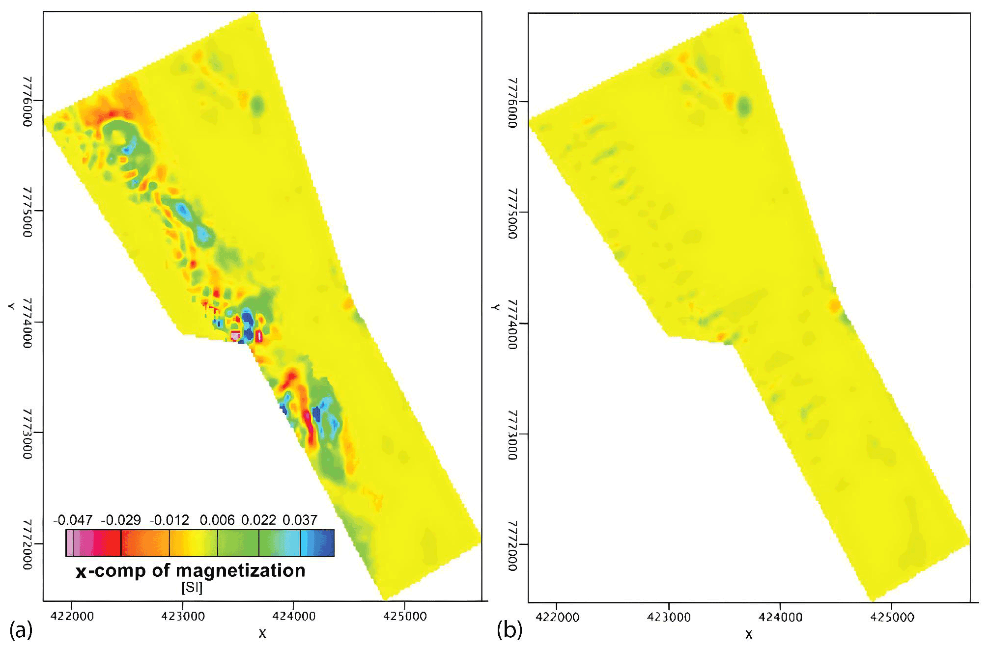
Figure C2X components of the magnetization 50 m below the surface are shown for the two constrained inversion tests. In (a) cells associated with sediment units were constrained towards a non-magnetic reference model (see Figs. 6 and 7), but in (b) in addition the direction of the magnetization in the magmatic units is constrained towards the direction of the regional magnetic field (see Fig. C1).
Referring to Riisager and Abrahamsen (1999, 2000), the palaeomagnetic field direction of the Asuk Member can be estimated with an inclination and declination of −80.7 and 228.1∘, respectively. The present-day Earth magnetic field direction (IGRF) at Qullissat had during the field campaign an inclination of 81∘ and a declination of −31.5∘ resulting in an angle of ∼ 168.3∘ between the two fields.
Accordingly, we assumed that the induced and the remanent magnetization are approximately parallel or antiparallel in most locations. We considered these main magnetization directions in the magmatic units by keeping the components perpendicular to the Earth magnetic field small. This was achieved by modifying the weights w0 (basalt) of ϕM, Ref and having non-zero weights of 0.125 in the direction perpendicular to the current Earth magnetic field such that zero-weights only remained in the direction of the Earth magnetic field for the basalts and the magmatic body. Since the weights had to be expressed in the coordinate system used for the model (x = east, y = north, z = height), a rotation was applied onto the weighting factors resulting in (0.124, 0.123, 0.0196). Rather small weights were selected with 0.125, since there is a higher uncertainty with the assumed magnetization direction.
Results of this test are presented in Fig. C1. As for the former inversion test, in which only the sediment units were constrained, higher magnetization values are accumulated in cells associated with the magmatic units and both positive and negative anomalies appear. The only anomalies located outside of this volume are again the anomalies A and B. In contrast to the former inversion run, the x and y components have rather small values within areas assigned to the magmatic units (Fig. C2) such that almost the whole magnetization is associated with the z component. In addition, the absolute magnetization values are generally higher but are usually not >0.4 SI (maximum value is 0.6 SI), and general orientations in a N–S to NNW–SSE direction are less pronounced (Fig. C1) than in the former test, but anomalies are more scattered and generally smaller in scale.
The original data of the study are available upon provision of a valid request.
RJ, RZ, BHH, HS and UK designed the survey and conducted field work. RJ wrote the draft with support of BHH, EVS, SL, RZ and MK. RJ constructed Figs. 1–4, 8–10 and 12–14 and integrated all data. BHH conducted the inversion and built Figs. 5–7, C1 and C2. SL provided SEM analysis and Fig. 11. RZ with RJ acquired UAS data. RJ processed and analysed spectral and optical UAS and surface sample data. HS processed ground magnetics. MP processed magnetic UAS data. All authors took part in the discussion of the results, interpretation and review. BHH and RG supervised the project and acquired funding.
The contact author has declared that neither they nor their co-authors have any competing interests.
Publisher’s note: Copernicus Publications remains neutral with regard to jurisdictional claims in published maps and institutional affiliations.
This article is part of the special issue “State of the art in mineral exploration”. It is a result of the EGU General Assembly 2020, 3–8 May 2020.
We thank BlueJay Mining PLC for their support during the preparation and conduction of the field campaign. In particular, we thank Bo Møller Stensgaard and Hans Jensen for logistic support. We thank Radai Oy, especially Arto Karinen, Lauri Maalismaa and Ari Saartenoja, for the UAS magnetic measurements. We thank GEUS for preparation of the field campaign. Lotte Larsen (GEUS), Asger Pedersen (GEUS) and Ethan Barnes are gratefully thanked for the fruitful geologic discussions. We thank Satu Mertanen from GTK petrophysical labs and Kai Bachmann from the Erzlabor at HZDR-HIF for sample preparations and measurements. We thank the Seequent Team for providing us with relevant information about their MVI inversion tool. We thank the anonymous referees for their helpful comments. MULSEDRO's field campaign was conducted under scientific survey licence (VU-00158-2019) within mineral exploration licence MEL 2018-16 by Blue Jay Mining PLC.
This research has been supported by the project MULSEDRO, funded by EITRawMaterials (project ID 16193)
and the European Union organization EIT. Blue Jay Mining
PLC supported the SEM analysis.
The article processing charges for this open-access publication were covered by the Helmholtz-Zentrum Dresden-Rossendorf (HZDR).
This paper was edited by Alba Gil de la Iglesia and reviewed by two anonymous referees.
Airo, M.-L. and Säävuori, H.: Petrophysical characteristics of Finnish bedrock, Geol. Surv. Finland, Espoo, Report of Investigation 205, ISBN 978-952-217-267-9, 35 pp., 2013.
Athavale, R. N. and Sharma, P. V.: Paleomagnetic Results on Early Tertiary Lava Flows from West Greenland and their bearing on the Evolution History of the Baffin Bay–Labrador Sea Region, Can. J. Earth Sci., 12, 1–18, https://doi.org/10.1139/e75-001, 1975.
Austin, J. and Crawford, B.: Remanent magnetization mapping: A tool for greenfields magmatic Ni-Cu-PGE exploration undercover: Part 1, Ore Geol. Rev., 107, 457–475, https://doi.org/10.1016/j.oregeorev.2019.03.008, 2019.
Barnes, S. J., Cruden, A. R., Arndt, N., and Saumur, B. M.: The mineral system approach applied to magmatic Ni–Cu–PGE sulphide deposits, Ore Geol. Rev., 76, 296–316, https://doi.org/10.1016/j.oregeorev.2015.06.012, 2016.
Bedini, E.: Mineral mapping in the Kap Simpson complex, central East Greenland, using HyMap and ASTER remote sensing data, Adv. Space Res., 47, 60–73, https://doi.org/10.1016/j.asr.2010.08.021, 2011.
Bedini, E. and Rasmussen, T. M.: Use of airborne hyperspectral and gamma-ray spectroscopy data for mineral exploration at the Sarfartoq carbonatite complex, southern West Greenland, Geosci. J., 22, 641–651, https://doi.org/10.1007/s12303-017-0078-5, 2018.
Bird, J. M. and Weathers, M. S.: Native iron occurrences of Disko Island, Greenland, J. Geol., 85, 359–371, 1977.
Blakely, R. J.: Potential Theory in Gravity and Magnetic Applications, Cambridge University Press, Cambridge, https://doi.org/10.1017/CBO9780511549816, 1995.
Blue Jay Mining PLC: Results of MMI and SGH Geochemical Surveys at the Disko-Nuussuaq Project and Licence Expansion, press release, https://www.rns-pdf.londonstockexchange.com/rns/8283B_1-2020-2-3.pdf, last access: 11 October 2021.
Bonow, J. M., Japsen, P., Lidmar-Bergström, K., Chalmers, J. A., and Pedersen, A. K.: Cenozoic uplift of Nuussuaq and Disko, West Greenland – elevated erosion surfaces as uplift markers of a passive margin, Geomorphology, 80, 325–337, 2006.
Booysen, R., Jackisch, R., Lorenz, S., Zimmermann, R., Kirsch, M., Nex, P. A. M., and Gloaguen, R.: Detection of REEs with lightweight UAV-based hyperspectral imaging, Sci. Rep., 10, 17450, https://doi.org/10.1038/s41598-020-74422-0, 2020.
Brethes, A., Guarnieri, P., and Rasmussen, T. M.: Integrating 3D photogeology with aeromagnetic data as a tool for base-metal exploration in East Greenland, GEUS Bull., 31, 71–74, https://doi.org/10.34194/geusb.v31.4664, 2014.
Brethes, A., Guarnieri, P., Rasmussen, T. M., and Bauer, T. E.: Interpretation of aeromagnetic data in the Jameson Land Basin, central East Greenland: Structures and related mineralized systems, Tectonophysics, 724/725, 116–136, https://doi.org/10.1016/j.tecto.2018.01.008, 2018.
Calou, P. and Munschy, M.: Airborne Magnetic Surveying with a Drone and Determination of the Total Magnetization of a Dipole, IEEE Trans. Magn., 56, 6000409, https://doi.org/10.1109/TMAG.2020.2986988, 2020.
Cande, S. C. and Kent, D. V.: Revised calibration of the geomagnetic polarity timescale for the Late Cretaceous and Cenozoic, J. Geophys. Res.-Sol. Ea., 100, 6093–6095, https://doi.org/10.1029/94JB03098, 1995.
Chalmers, J. A., Pulvertaft, T. C. R., Marcussen, C., and Pedersen, A. K.: New insight into the structure of the Nuussuaq Basin, central West Greenland, Mar. Petrol. Geol., 16, 197–211, https://doi.org/10.1016/S0264-8172(98)00077-4, 1999.
Clark, D.: Magnetic petrophysics and magnetic petrology: Aids to geological interpretation of magnetic surveys, AGSO J. Austr. Geol. Geophys., 17, 83–104, 1997.
Clark, D. A. and Emerson, J. B.: Notes On Rock Magnetization Characteristics In Applied Geophysical Studies, Explor. Geophys., 22, 547–555, https://doi.org/10.1071/EG991547, 1991.
Crowley, J. K., Williams, D. E., Hammarstrom, J. M., Piatak, N., Chou, I.-M., and Mars, J. C.: Spectral reflectance properties (0.4–2.5 µm) of secondary Fe-oxide, Fe-hydroxide, and Fe-sulphate-hydrate minerals associated with sulphide-bearing mine wastes, Geochemi. Explor. Environ. Anal., 3, 219–228, https://doi.org/10.1144/1467-7873/03-001, 2003.
Cunningham, M., Samson, C., Wood, A., and Cook, I.: Aeromagnetic Surveying with a Rotary-Wing Unmanned Aircraft System: A Case Study from a Zinc Deposit in Nash Creek, New Brunswick, Canada, Pure Appl. Geophys., 175, 3145–3158, https://doi.org/10.1007/s00024-017-1736-2, 2018.
Dahl-Jensen, T., Larsen, L. M., Pedersen, S. A. S., Pedersen, J., Jepsen, H. F., Pedersen, G., Nielsen, T., Pedersen, A. K., Von Platen-Hallermund, F., and Weng, W.: Landslide and Tsunami 21 November 2000 in Paatuut, West Greenland, Nat. Hazards, 31, 277–287, https://doi.org/10.1023/B:NHAZ.0000020264.70048.95, 2004.
Dam, G., Pedersen, G. K., Sønderholm, M., Midtgaard, H. H., Larsen, L. M., Nøhr-Hansen, H., and Pedersen, A. K.: Lithostratigraphy of the Cretaceous-Paleocene Nuussuaq group, Nuussuaq basin, West Greenland, Geological Survey of Denmark and Greenland Bulletin, ISBN 978-87-7871-260-8, 1–171, 2009.
Data, E., Donohue, J., and Legault, J.: Geological report regarding the Quantec TITAN-24 distributed Array System Tensor-magnetotelluric survey over the Disko Project, Greenland, during 2004, on behalf of Vismand Exploration Inc., Geological Survey of Denmark and Greenland, GEUS internal report file 21888, 14 pp., 2005.
Dataforsyningen: Danish Agency for Data Supply and Efficiency: SDFE pilotprojekt “Nykortlægning af Grønland”, https://dataforsyningen.dk/data/2842 (last access: 21 May 2021), 2019.
Dentith, M. and Mudge, S. T.: Geophysics for the Mineral Exploration Geoscientist, Cambridge University Press, Cambridge, UK, 454 pp., https://doi.org/10.1017/CBO9781139024358, 2014.
Dering, G. M., Micklethwaite, S., Thiele, S. T., Vollgger, S. A., and Cruden, A. R.: Review of drones, photogrammetry and emerging sensor technology for the study of dykes: Best practises and future potential, J. Volcanol. Geoth. Res., 373, 148–166, https://doi.org/10.1016/j.jvolgeores.2019.01.018, 2019.
Deutsch, E. R. and Kristjansson, L. G.: Palaeomagnetism of Late Cretaceous-Tertiary Volcanics from Disko Island, West Greenland, Geophys. J. Roy. Astron. Soc., 39, 343–360, https://doi.org/10.1111/j.1365-246X.1974.tb05459.x, 1974.
Dunlop, D. J. and Argyle, K. S.: Thermoremanence, anhysteretic remanence and susceptibility of submicron magnetites: Nonlinear field dependence and variation with grain size, J. Geophys. Res.-Sol. Ea., 102, 20199–20210, https://doi.org/10.1029/97JB00957, 1997.
Ellis, R., de Wet, B., and Macleod, I.: Inversion of Magnetic Data from Remanent and Induced Sources, in: ASEG Extended Abstracts, 22nd ASEG International Geophysical Conference and Exhibition, Brisbane, Australia, 26–29 February 2016, 1–4, https://doi.org/10.1071/ASEG2012ab117, 2012.
Flores, H., Lorenz, S., Jackisch, R., Tusa, L., Contreras, I. C., Zimmermann, R., and Gloaguen, R.: UAS-Based Hyperspectral Environmental Monitoring of Acid Mine Drainage Affected Waters, Minerals, 11, 182, https://doi.org/10.3390/min11020182, 2021.
Gavazzi, B., Le Maire, P., Munschy, M., and Dechamp, A.: Fluxgate vector magnetometers: A multisensor device for ground, UAV, and airborne magnetic surveys, Leading Edge, 35, 795–797, https://doi.org/10.1190/tle35090795.1, 2016.
Gavazzi, B., Le Maire, P., Mercier de Lépinay, J., Calou, P., and Munschy, M.: Fluxgate three-component magnetometers for cost-effective ground, UAV and airborne magnetic surveys for industrial and academic geoscience applications and comparison with current industrial standards through case studies, Geomech. Energ. Environ., 20, 100117, https://doi.org/10.1016/j.gete.2019.03.002, 2019.
GDAL/OGR contributors: GDAL/OGR Geospatial Data Abstraction software Library, Open Source Geospatial Foundation, Zenodo [code], https://doi.org/10.5281/zenodo.6352176, 2021.
Government of Greenland: License map, https://govmin.gl, last access: 5 October 2021.
Gunn, P. J. and Dentith, M.: Magnetic responses associated with mineral deposits, AGSO J. Austral. Geol. Geophys., 17, 145–158, 1997.
Henderson, G., Schiener, E. J., Risum, J. B., Croxton, C. A., and Andersen, B. B.: The West Greenland Basin, in: Geology of the North Atlantic borderlands, Vol. 7, edited by: Escher, A. and Watt, W. S., Memoir Canadian Society of Petroleum Geologists, 1981.
Howarth, G. H., Day, J. M. D., Pernet-Fisher, J. F., Goodrich, C. A., Pearson, D. G., Luo, Y., Ryabov, V. V., and Taylor, L. A.: Precious metal enrichment at low-redox in terrestrial native Fe-bearing basalts investigated using laser-ablation ICP-MS, Geochim. Cosmochim. Ac., 203, 343–363, https://doi.org/10.1016/j.gca.2017.01.003, 2017.
Hungr, O., Leroueil, S., and Picarelli, L.: The Varnes classification of landslide types, an update, Landslides, 11, 167–194, 2014.
Hunt, G. R. and Ashley, R. P.: Spectra of altered rocks in the visible and near infrared, Econ. Geol., 74, 1613–1629, https://doi.org/10.2113/gsecongeo.74.7.1613, 1979.
Isles, D. J. and Rankin, L. R.: Geological interpretation of aeromagnetic data, 1st Edn., Society of Exploration Geophysicists and Australian Society of Exploration, Australia, 365 pp., https://doi.org/10.1190/1.9781560803218, 2013.
Jackisch, R., Madriz, Y., Zimmermann, R., Pirttijärvi, M., Saartenoja, A., Heincke, B. H., Salmirinne, H., Kujasalo, J.-P., Andreani, L., and Gloaguen, R.: Drone-borne hyperspectral and magnetic data integration: Otanmäki Fe-Ti-V deposit in Finland, Remote Sens., 11, 2084, https://doi.org/10.3390/rs11182084, 2019.
Jackisch, R., Lorenz, S., Kirsch, M., Zimmermann, R., Tusa, L., Pirttijärvi, M., Saartenoja, A., Ugalde, H., Madriz, Y., Savolainen, M., and Gloaguen, R.: Integrated geological and geophysical mapping of a carbonatite-hosting outcrop in Siilinjärvi, Finland, using unmanned aerial systems, Remote Sens., 12, 2998, https://doi.org/10.3390/RS12182998, 2020.
Jakob, S., Zimmermann, R., and Gloaguen, R.: The Need for Accurate Geometric and Radiometric Corrections of Drone-Borne Hyperspectral Data for Mineral Exploration: MEPHySTo-A Toolbox for Pre-Processing Drone-Borne Hyperspectral Data, Remote Sens., 9, 1–17, https://doi.org/10.3390/rs9010088, 2017.
James, M. R. and Robson, S.: Mitigating systematic error in topographic models derived from UAV and ground-based image networks, Earth Surf. Process. Land., 39, 1413–1420, 2014.
James, M. R., Robson, S., D'Oleire-Oltmanns, S., and Niethammer, U.: Optimising UAV topographic surveys processed with structure-from-motion: Ground control quality, quantity and bundle adjustment, Geomorphology, 280, 51–66, https://doi.org/10.1016/j.geomorph.2016.11.021, 2017.
James, M. R., Chandler, J. H., Eltner, A., Fraser, C., Miller, P. E., Mills, J. P., Noble, T., Robson, S., and Lane, S. N.: Guidelines on the use of structure-from-motion photogrammetry in geomorphic research, Earth Surf. Process. Land., 2084, 2081–2084, https://doi.org/10.1002/esp.4637, 2019.
Japsen, P., Green, P. F., and Chalmers, J. A.: Separation of Palaeogene and Neogene uplift on Nuussuaq, West Greenland, J. Geol. Soc., 162, 299–314, 2005.
Keays, R. R. and Lightfoot, P. C.: Siderophile and chalcophile metal variations in Tertiary picrites and basalts from West Greenland with implications for the sulphide saturation history of continental flood basalt magmas, Miner. Deposita, 42, 319–336, https://doi.org/10.1007/s00126-006-0112-4, 2007.
Kirsch, M., Lorenz, S., Zimmermann, R., Tusa, L., Möckel, R., Hödl, P., Booysen, R., Khodadadzadeh, M., and Gloaguen, R.: Integration of Terrestrial and Drone-Borne Hyperspectral and Photogrammetric Sensing Methods for Exploration Mapping and Mining Monitoring, Remote Sens., 10, 1366, https://doi.org/10.3390/rs10091366, 2018.
Kriegler, F. J., Malila, W. A., Nalepka, R. F., and Richardson, W.: Preprocessing transformations and their effects on multispectral recognition, in: Proceedings of the Sixth International Symposium on Remote Sensing of Environment, Sixth International Symposium on Remote Sensing of Environment, Ann Arbor, MI, 97–131, 1969.
Larsen, L. M. and Pedersen, A. K.: Petrology of the paleocene picrites and flood basalts on Disko and Nuussuaq, West Greenland, J. Petrol., 50, 1667–1711, https://doi.org/10.1093/petrology/egp048, 2009.
Larsen, L. M., Pedersen, A. K., Tegner, C., Duncan, R. A., Hald, N., and Larsen, J. G.: Age of Tertiary volcanic rocks on the West Greenland continental margin: volcanic evolution and event correlation to other parts of the North Atlantic Igneous Province, Geol. Mag., 153, 487–511, https://doi.org/10.1017/S0016756815000515, 2016.
Le Maire, P., Bertrand, L., Munschy, M., Diraison, M., and Géraud, Y.: Aerial magnetic mapping with an unmanned aerial vehicle and a fluxgate magnetometer: a new method for rapid mapping and upscaling from the field to regional scale, Geophys. Prospect., 68, 2307–2319, https://doi.org/10.1111/1365-2478.12991, 2020.
Li, Y., Sun, J., Li, S.-L., and Leão-Santos, M.: A paradigm shift in magnetic data interpretation: Increased value through magnetization inversions, Leading Edge, 40, 89–98, https://doi.org/10.1190/tle40020089.1, 2021.
Lightfoot, P. C. and Hawkesworth, C. J.: Flood Basalts and Magmatic Ni, Cu, and PGE Sulphide Mineralization: Comparative Geochemistry of the Noril'sk (Siberian Traps) and West Greenland Sequences, in: Large Igneous Provinces: Continental, Oceanic, and Planetary Flood Volcanism, edited by: Mahoney, J. J. and Coffin, M. F., American Geophysical Union (AGU), 357–380, https://doi.org/10.1029/GM100p0357, 1997.
Lightfoot, P. C., Hawkesworth, C. J., Olshefsky, K., Green, T., Doherty, W., and Keays, R. R.: Geochemistry of Tertiary tholeiites and picrites from Qeqertarssuaq (Disko Island) and Nuussuaq, West Greenland with implications for the mineral potential of co-magmatic intrusions, Contrib. Mineral. Petr., 128, 139–163, https://doi.org/10.1007/s004100050300, 1997.
Liu, S., Hu, X., Zhang, H., Geng, M., and Zuo, B.: 3D Magnetization Vector Inversion of Magnetic Data: Improving and Comparing Methods, Pure Appl. Geophys., 174, 4421–4444, https://doi.org/10.1007/s00024-017-1654-3, 2017.
MacLeod, I. N. and Ellis, R. G.: Magnetic vector inversion, a simple approach to the challenge of varying direction of rock magnetization, in: ASEG Extended Abstracts, 23rd International Geophysical Conference and Exhibition, Melbourne, Australia, 11–14 August 2013, 1–6, 2013.
MacLeod, I. N. and Ellis, R. G.: Quantitative magnetization vector inversion, in: ASEG Extended Abstracts, 25th International Conference and Exhibition – Interpreting the Past, Discovering the Future, Adelaide, Australia, 21–24 August 2016, 1–5, 2016.
Malehmir, A., Dynesius, L., Paulusson, K., Paulusson, A., Johansson, H., Bastani, M., Wedmark, M., and Marsden, P.: The potential of rotary-wing UAV-based magnetic surveys for mineral exploration: A case study from central Sweden, Leading Edge, 36, 552–557, https://doi.org/10.1190/tle36070552.1, 2017.
Miller, C. A., Schaefer, L. N., Kereszturi, G., and Fournier, D.: Three-Dimensional Mapping of Mt. Ruapehu Volcano, New Zealand, From Aeromagnetic Data Inversion and Hyperspectral Imaging, J. Geophys. Res.-Sol. Ea., 125, 1–24, https://doi.org/10.1029/2019JB018247, 2020.
Miller, H. G. and Singh, V.: Potential field tilt – a new concept for location of potential field sources, J. Appl. Geophys., 32, 213–217, https://doi.org/10.1016/0926-9851(94)90022-1, 1994.
Nabighian, M. N.: The Analytic Signal Of Two-Dimensional Magnetic Bodies With Polygonal Cross-Section: Its Properties And Use For Automated Anomaly Interpretation, Geophysics, 37, 507–517, https://doi.org/10.1190/1.1440276, 1972.
Nabighian, M. N., Grauch, V. J. S., Hansen, R. O., LaFehr, T. R., Li, Y., Peirce, J. W., Phillips, J. D., and Ruder, M. E.: The historical development of the magnetic method in exploration, Geophysics, 70, 33–61, https://doi.org/10.1190/1.2133784, 2005.
Nagata, T., Ishikawa, Y., Kinoshita, H., Kono, M., Syono, Y., and Fisher, R. M.: Magnetic properties and natural remanent magnetization of lunar materials, in: Geochimica et Cosmochimica Acta Supplement, Proceedings of the Apollo 11 Lunar Science Conference, Houston, TX, 2325, 1970.
Nakatsuka, T. and Okuma, S.: Reduction of Magnetic Anomaly Observations from Helicopter Surveys at Varying Elevations, Explor. Geophys., 37, 121–128, https://doi.org/10.1071/EG06121, 2006.
Olshefsky, K.: Falconbridge Limited – Report of 1991 Exploration Activities, West Greenland Tertiary Basalt Province for Prospecting License #156 and Exploration Concession #165, Geological Survey of Denmark and Greenland, Copenhagen, Report file no. 21092, 165 pp., 1992.
Olshefsky, K. and Jerome, M.: Falconbridge Limited – Report of 1992 Exploration Activities, West Greenland Tertiary Basalt Province for Prospecting License #156 and exploration licenses 02/91, 03/91, 04/91, 25/92, Geological Survey of Denmark and Greenland, Copenhagen, Report file no. 21216, 300 pp., 1993.
Olshefsky, K. and Jerome, M.: Falconbridge Limited – West Greenland Tertiary Basalt Province; Report of 1993 Exploration Activities for Prospecting License #156 and exploration licenses 02/91, 03/91, Geological Survey of Denmark and Greenland, Copenhagen, Report file no. 21356, 333 pp., 1994.
Olshefsky, K., Jerome, M., and Graves, M.: Falconbridge Limited A/S – West Greenland Tertiary Basalt Province; Report of 1994 Exploration Activities for Prospecting License 06/94 and exploration licenses 02/91 & 03/91, Geological Survey of Denmark and Greenland, Copenhagen, Report file no. 21410, 326 pp., 1995.
Park, S. and Choi, Y.: Applications of unmanned aerial vehicles in mining from exploration to reclamation: A review, Minerals, 10, 663, https://doi.org/10.3390/min10080663, 2020.
Parshin, A. V., Morozov, V. A., Blinov, A. V., Kosterev, A. N., and Budyak, A. E.: Low-altitude geophysical magnetic prospecting based on multirotor UAV as a promising replacement for traditional ground survey, Geo-spatial Inf. Sci., 21, 67–74, https://doi.org/10.1080/10095020.2017.1420508, 2018.
Pauly, H.: Igdlukúnguaq nickeliferous pyrrhotite; texture and composition. A contribution to the genesis of the ore type., Bianco Lunos Bogtrykkeri, Copenhagen, Denmark, 169 pp., 1958.
Pedersen, A.: Iron-bearing and related volcanic rocks in the area between Gieseckes Dal and Hammers Dal, north-west Disko, Rapp. Gronlands Geol. Unders, 81, 5–14, 1977.
Pedersen, A. K.: Lithostratigraphy of the Tertiary Vaigat Formation on Disko, central West Greenland, Geological Survey of Denmark and Greenland, Copenhagen, Report file no. 22461, 33 pp., 1985.
Pedersen, A. K., Larsen, L. M., and Pedersen, G. K.: Lithostratigraphy, geology and geochemistry of the volcanic rocks of the Vaigat Formation on Disko and Nuussuaq, Paleocene of West Greenland, Geol. Surv. Den. Greenl., 39, 244 pp., https://doi.org/10.34194/geusb.v39.4354, 2017.
Pedersen, A. K., Larsen, L. M., and Pedersen, G. K.: Lithostratigraphy, geology and geochemistry of the volcanic rocks of the Maligât Formation and associated intrusions on Disko and Nuussuaq, Paleocene of West Greenland, Geol. Surv. Den. Greenl., 40, 239 pp., https://doi.org/10.34194/geusb.v40.4326, 2018.
Pedersen, M., Weng, W. L., Keulen, N., and Kokfelt, T. F.: A new seamless digital 1 : 500 000 scale geological map of Greenland, GEUS Bulletin, 28, 65–68, https://doi.org/10.34194/geusb.v28.4727, 2013.
Pernet-Fisher, J. F., Day, J. M. D., Howarth, G. H., Ryabov, V. V., and Taylor, L. A.: Atmospheric outgassing and native-iron formation during carbonaceous sediment–basalt melt interactions, Earth Planet. Sc. Lett., 460, 201–212, https://doi.org/10.1016/j.epsl.2016.12.022, 2017.
Pirttijärvi, M.: Numerical modeling and inversion of geophysical electromagnetic measurements using a thin plate model, PhD dissertation, University of Oulu, Oulu, Finland, 44 pp., ISBN 951-42-7118-1, 2003.
Planet Team: Planet Application Program Interface: In Space for Life on Earth [data set], San Francisco, CA, https://api.planet.com (last access: 21 November 2020), 2017.
Plouffe, A., Anderson, R. G., Gruenwald, W., Davis, W. J., Bednarski, J. M., and Paulen, R. C.: Integrating ice-flow history, geochronology, geology, and geophysics to trace mineralized glacial erratics to their bedrock source: An example from south-central British Columbia, Can. J. Earth Sci., 48, 1113–1129, 2011.
Porter, C., Morin, P., Howat, I., Noh, M.-J., Bates, B., Peterman, K., Keesey, S., Schlenk, M., Gardiner, J., Tomko, K., Willis, M., Kelleher, C., Cloutier, M., Husby, E., Foga, S., Nakamura, H., Platson, M., Wethington, M., Jr., Williamson, C., Bauer, G., Enos, J., Arnold, G., Kramer, W., Becker, P., Doshi, A., D'Souza, C., Cummens, P., Laurier, F., and Bojesen, M.: ArcticDEM, Harvard Dataverse [data set], V1, https://doi.org/10.7910/DVN/OHHUKH, 2018.
Portniaguine, O. and Zhdanov, M. S.: 3-D magnetic inversion with data compression and image focusing, Geophysics, 67, 1532–1541, https://doi.org/10.1190/1.1512749, 2002.
Puranen, M. and Puranen, R.: Apparatus for the measurement of magnetic susceptibility and its anisotropy, Report of Investigation, Geol. S. Finl., 28, 46 pp., 1977.
Ren, H., Zhao, Y., Xiao, W., and Hu, Z.: A review of UAV monitoring in mining areas: current status and future perspectives, Int. J. Coal Sci. Technol., 6, 320–333, https://doi.org/10.1007/s40789-019-00264-5, 2019.
Riisager, P. and Abrahamsen, N.: Magnetostratigraphy of Palaeocene basalts from the Vaigat Formation of West Greenland, Geophys. J. Int., 137, 774–782, https://doi.org/10.1046/j.1365-246X.1999.00830.x, 1999.
Riisager, P. and Abrahamsen, N.: Palaeointensity of West Greenland Palaeocene basalts: asymmetric intensity around the C27n–C26r transition, Phys. Earth Planet. In., 118, 53–64, https://doi.org/10.1016/S0031-9201(99)00125-9, 2000.
Roest, W. R., Verhoef, J., and Pilkington, M.: Magnetic interpretation using the 3-D analytic signal, Geophysics, 57, 116–125, https://doi.org/10.1190/1.1443174, 1992.
Rosa, D., Stensgaard, B. M., and Sørensen, L. L.: Magmatic nickel potential in Greenland Reporting the mineral ressource assessement workshop 27-29 November 2012, Danmarks og Grønlands Geologiske Undersøgelse Rapport, GEUS, Copenhagen, Report file no. 2013/57, 135 pp., 2013.
Rowan, L. C. and Mars, J. C.: Lithologic mapping in the Mountain Pass, California area using Advanced Spaceborne Thermal Emission and Reflection Radiometer (ASTER) data, Remote Sens. Environ., 84, 350–366, https://doi.org/10.1016/S0034-4257(02)00127-X, 2003.
Rowan, L. C., Mars, J. C., and Simpson, C. J.: Lithologic mapping of the Mordor, NT, Australia ultramafic complex by using the Advanced Spaceborne Thermal Emission and Reflection Radiometer (ASTER), Remote Sens. Environ., 99, 105–126, 2005.
Salehi, S., Rogge, D., Rivard, B., Heincke, B. H., and Fensholt, R.: Modeling and assessment of wavelength displacements of characteristic absorption features of common rock forming minerals encrusted by lichens, Remote Sens. Environ., 199, 78–92, https://doi.org/10.1016/j.rse.2017.06.044, 2017.
Sørensen, L. L., Stensgaard, B. M., Thrane, K., Rosa, D., and Kalvig, P.: Sediment-hosted zinc potential in Greenland Reporting the mineral resource assessment workshop 29 November–1 December 2011, Danmarks og Grønlands Geologiske Undersøgelse Rapport, GEUS, Copenhagen, Report file no. 2013/56, 184 pp., 2013.
Steenstrup, K. J. V.: Beretning om en Undersøgelsesrejse til Øen Disko i Sommeren 1898, 24, Bianco Lunos Bogtrykkeri, Copenhagen, Denmark, 249–306, 1901.
Svennevig, K.: Preliminary landslide mapping in Greenland, Geol. Surv. Den. Greenl., 43, 1–5, https://doi.org/10.34194/GEUSB-201943-02-07, 2019.
Thorning, L. and Stemp, R. W.: Airborne geophysical surveys in central West Greenland and central East Greenland in 1997, Geol. Surv. Den. Greenl., 180, 63–66, https://doi.org/10.34194/ggub.v180.5087, 1998.
Ulff-Møller, F.: Native iron bearing intrusions of the Hammersdal complex, North-West Disko, Gronlands Geologiske Undersogelse Rapport, 81, 15–33, GEUS, https://doi.org/10.34194/rapggu.v81.7511, 1977.
Ulff-Møller, F.: Solidification History of the KitdlÎt Lens: Immiscible Metal and Sulphide Liquids from a Basaltic Dyke on Disko, Central West Greenland, J. Petrol., 26, 64–91, https://doi.org/10.1093/petrology/26.1.64, 1985.
Ulff-Møller, F.: A new 10 tons iron boulder from Disko, West Greenland, Meteoritics, 21, 464, GEUS, 1986.
Ulff-Møller, F.: Formation of native iron in sediment-contaminated magma: I. A case study of the Hanekammen Complex on Disko Island, West Greenland, Geochim. Cosmochim. Ac., 54, 57–70, https://doi.org/10.1016/0016-7037(90)90195-Q, 1990.
Vallée, M. A., Smith, R. S., and Keating, P.: Metalliferous mining geophysics — State of the art after a decade in the new millennium, Geophysics, 76, W31–W50, https://doi.org/10.1190/1.3587224, 2011.
Varnes, D. J.: Landslide types and processes, in: Landslides and Engineering Practice, Vol. 29, edited by: Eckel, E. B., Highway Research Board, Washington, D.C., 20–47, 1958.
Walter, C., Braun, A., and Fotopoulos, G.: High-resolution unmanned aerial vehicle aeromagnetic surveys for mineral exploration targets, Geophysical Prospecting, 68, 334–349, https://doi.org/10.1111/1365-2478.12914, 2020.
Weiss, A. D.: Topographic position and landforms analysis, ESRI International User conference, San Diego, CA, USA, 9–13 July 2001, 2001.
Zhdanov, M. S.: Geophysical inverse theory and regularization problems, 1st Edn., Elsevier Science, Amsterdam, Oxford, 633 pp., Elsevier, ISBN 978-0-444-51089-1, 2002.
Zheng, Y., Li, S., Xing, K., and Zhang, X.: Unmanned Aerial Vehicles for Magnetic Surveys: A Review on Platform Selection and Interference Suppression, Drones, 5, 93, https://doi.org/10.3390/drones5030093, 2021.
- Abstract
- Introduction
- Methods and materials
- Results
- Interpretation and discussion
- Conclusion and outlook
- Appendix A: Flight control and processing of UAS-based magnetic data
- Appendix B: Multispectral surveys
- Appendix C: Magnetic vector inversion with constrained magnetization directions
- Data availability
- Author contributions
- Competing interests
- Disclaimer
- Special issue statement
- Acknowledgements
- Financial support
- Review statement
- References