the Creative Commons Attribution 4.0 License.
the Creative Commons Attribution 4.0 License.
 | 29 Apr 2022
Establishing an integrated workflow identifying and linking surface and subsurface lineaments for mineral exploration under cover: example from the Gawler Craton, South Australia
Ulrich Kelka
Cericia Martinez
Carmen Krapf
Stefan Westerlund
Ignacio Gonzalez-Alvarez
Mark Pawley
Clive Foss
Mineral exploration in areas comprising thick and complex cover represents an intrinsic challenge. Cost- and time-efficient methods that help to narrow down exploration areas are therefore of particular interest to the Australian mining industry and for mineral exploration worldwide. Based on a case study around the Tarcoola gold mine in the regolith-dominated South Australian central Gawler Craton, we suggest an exploration targeting workflow based on the joint analysis of surface and subsurface lineaments. The datasets utilised in this study are a digital elevation model and radiometric data that represent surface signals and total magnetic intensity and gravity attributed to subsurface signals. We compare automatically and manually mapped lineament sets derived from remotely sensed data. In order to establish an integrated concept for exploration through cover based on the best-suited lineament data, we will point out the most striking differences between the automatically and manually detected lineaments and compare the datasets that represent surficial in contrast to subsurface structures. We further show how lineaments derived from surface and subsurface datasets can be combined to obtain targeting maps that help to narrow down areas for mineral exploration. We propose that target areas are represented by high lineament densities which are adjacent to regions comprising high density of lineament intersections.
- Article
(17584 KB) - Full-text XML
- BibTeX
- EndNote


The Gawler Craton (Fig. 1a) is one of the three largest Archean to Proterozoic Cratons within the Australian Continent (Fig. 1b) and the major crustal province in South Australia (Hand et al., 2007). Australian Cratons are rich in mineralisation (e.g. Pilbara and Yilgarn Craton Witt et al., 1998), and the Gawler Craton hosts significant economic mineralisation such as Olympic Dam, Challenger, Prominent Hill, and Tarcoola. The discovery of new deposits is particularly challenging in this part of Australia due to limited surface outcrops, variable thickness, and complexity of the cover, with few surface features that can be used as direct proxies for mineral exploration.
To narrow down potential areas for exploration, and to enhance the general understanding of the geology, the Geological Survey of South Australia (GSSA) has recently acquired high-resolution magnetic, radiometric, and digital elevation data across the Gawler Craton via the Gawler Craton Airborne Survey (GCAS) (Katona et al., 2019). Here we utilise these and previously acquired gravity datasets for the extraction of lineaments from the surface (digital elevation model (DEM) and radiometrics) and subsurface (magnetics and gravity) datasets. Lineaments are linear features that can reflect geological structures, and the extraction of such features can be important for mineral exploration, as well as for the investigation of fault activity (neotectonic) and water resource analysis (Vassilas et al., 2002). In images, photos, or maps, lineaments are represented by straight or slightly curved lines, linear patterns, or an alignment of discontinuity patterns (Wang, 1993). A relationship between lineaments and mineralisation has been suggested for a long time and has been proven to be a useful tool for mineral exploration (O'Driscoll, 1986). We can distinguish between surface lineaments that are obtained from surface data and geophysical lineaments that are derived from processed geophysical data. It is widely assumed that surface lineaments represent structural features which in the simplest model are related to dip-slip or strike-slip faults (Florinsky, 2016). This assumes that a considerable displacement is associated with faulting in the subsurface that leads to a detectable pattern on the surface (Boucher, 1997). In contrast, geophysical lineaments represent major subsurface boundaries (e.g. Hall, 1986; Langenheim and Hildenbrand, 1997) that are not necessarily associated with faults, but rather with lithological or petrophysical contrasts. It is important to note that datasets such as those based on digital elevation models and radiometrics represent only topographical variations and changes in chemical composition of the surface geology or cover respectively.
As a case study for mineral exploration, we choose an area in the South Australian central Gawler craton around the Tarcoola mine, an Au deposit mined for over 125 years (Daly et al., 1990). As the structurally controlled mineralisation often localises around discontinuity intersections (Wilson et al., 2018), this area represents a perfect study area for investigating the potential of surface and subsurface lineaments as a potential exploration targeting tool. The thick and complex cover (up to 500 m) overlying the basement units makes it particularly challenging to identify target areas, and a cost-efficient approach to exploration targeting is desirable in such a region. A great challenge is that surface impressions of non-vertical basement-hosted displacement structures can be offset compared to the location of the discontinuity in the basement. Furthermore, cross-strike features are likely associated with small-scale shear zones that will not be traceable in potential field data that image basement structures. A reliable interpretation of surface and subsurface lineament sets is particularity challenging in an old crustal block such as the Gawler Craton, and we consider the work presented here as a first attempt to unify a lineament-based workflow for exploration targeting in such an environment.
In this study, we use the above-mentioned new GCAS datasets to identify surface and subsurface lineament features and design a workflow to automatically extract and analyse these features. We assume that elevation and radiometric data relate to surficial features, while gravity and magnetics data represent structures below the cover. This study is part of a broader effort to geologically link basement architecture with surface linear features, landforms, and landscape variability in the central Gawler Craton (González-Álvarez et al., 2019, 2020, 2022a, 2022b). It is important to note that datasets such as digital elevation models, or radiometric data represent only the change in surface properties such as elevation or surface geology. These lineaments may or may not represent structures that extend into the subsurface. By using datasets that represent the subsurface (i.e. gravity and magnetics) lineaments extracted are directly representative of changes in the subsurface. The challenge is identifying (1) if the lineaments from any dataset are geologically meaningful and (2) if lineaments from surface and subsurface datasets represent the same structure (e.g. fault, lithological boundary).
Towards that end, we further explore the generation and use of targeting maps (i.e. a map generated to highlight areas with specific features) based on surface and subsurface lineaments. Targeting maps derived from lineament analysis are often based on the density of lineaments per unit area. Density maps combining subsurface lineaments (potential field data) and surface lineaments (digital elevation model and satellite imagery) were proposed as an exploration tool for groundwater (Epuh et al., 2020) and for mineral exploration (Mohammadpour et al., 2020). Lineament intersections were also used previously for the analysis of groundwater (Ilugbo and Adebiyi, 2017), and locations of intersecting structural elements were suggested to represent favourable target areas for mineral exploration (Krapf and González-Álvarez, 2018; González-Álvarez et al., 2019; Sheikhrahimi et al., 2019; González-Álvarez et al., 2020, 2022b). In hydrocarbon exploration, cross-strike discontinuities were suggested as an exploration tool for natural gas (Wheeler, 1980). In the context of this contribution, we define targeting maps as maps which highlight areas that comprise the structural features preferable for mineral exploration.
We apply edge enhancement filtering to digital elevation data and perform manual lineament extraction on the DEM and automatic segmentation on all datasets to compare both approaches and results. We discuss the advantages and shortcomings of different edge detection filters applied to the subsurface and surface datasets and present a workflow (Fig. 1c) to help with the identification of linear features that could be linked to the main basement geological features.
The Gawler Craton is the oldest and largest geological province in South Australia and represents one of the three major Australian Cratons (Fig. 1b). The region hosts several economic iron-oxide copper-gold ore deposits (IOCG) including the world-class Olympic Dam (Fig. 1a). The Olympic IOCG province forms a 100 to 200 km wide north–south-trending belt at the eastern margin of the Gawler Craton (Skirrow et al., 2007). The largest known mineral occurrence in the area investigated is the Tarcoola mine, which hosts disseminated or veinlet-type Au- mineralisation mainly in brittle to brittle–ductile faults and shears (Hand et al., 2007). The age of the Tarcoola Au mineralisation is considered to be 1564 Ma (Bockmann et al., 2019), and the timing of the ore formation at the Tunkilla project (approx. 70 km S/SE of Tarcoola) has been constrained at 1590–1570 Ma (Budd and Fraser, 2004). Ongoing exploration in the central Gawler Craton targets Au, Cu-Au, Pb-Zn, Fe, and Ni in the crystalline basement (Sheard et al., 2008). The expected commodities within the investigated region are mainly Au and Fe and are likely located in proximity to crustal-scale structures that provided conduits for the upwelling of deep crustal fluids. Such large-scale reactivated tectonic features often form major crustal boundaries that are detectable with potential-field methods (Motta et al., 2019). It was shown that Archean gold mineralisations are often associated with such crustal-scale shear zones (Eisenlohr et al., 1989; Budd and Fraser, 2004). If a surface expression of such structures exists, this may be indicative that the crustal structures remained active for a long time resulting in a high amount of deformation or strong lithological contrasts. In the framework of the central Gawler mineral systems, the vicinity of such structures indicates potential exploration targets.
Three major orogenic events, corresponding to crustal deformation and tectono-thermal alterations, are recorded by the crystalline basement of the Gawler Craton: the Sleaford Orogeny (Paleoproterozoic, 2440 Ma), the Kimban Orogeny (Paleoproterozoic, 1845–1700 Ma), and the Kararan Orogeny (Mesoproterozoic, 1650–1540 Ma) (Ferris et al., 2002; Swain et al., 2005; Kositcin, 2010; Reid et al., 2014). Three major mineral systems are related to these three deformation–magmatic events, and the Tarcoola mineral field is attributed only to the Kararan system (≈ 1570 Ma) (Gum, 2019). As outlined by Hand et al. (2007), the exact timing and spatial distribution of the tectonostratigraphic sequences within the Gawler Craton remain a controversy, and reworking of existing mineralisation during reactivation of existing crustal-scale fluid conduits must be considered (Gum, 2019). The last large-scale deformation in the Gawler Craton was the reactivation of shear zones between 1470 and 1450 Ma (Hand et al., 2007). After this time, only minor near-surface movements are recorded (Sheard et al., 2008). Given the mineralisation is linked to the youngest orogeny in the area (Kararan Orogeny) and only minor tectonic activity is evident in the area after this event, we can assume that links between surficial and subsurface features point to areas of high deformation and/or neotectonic activity.
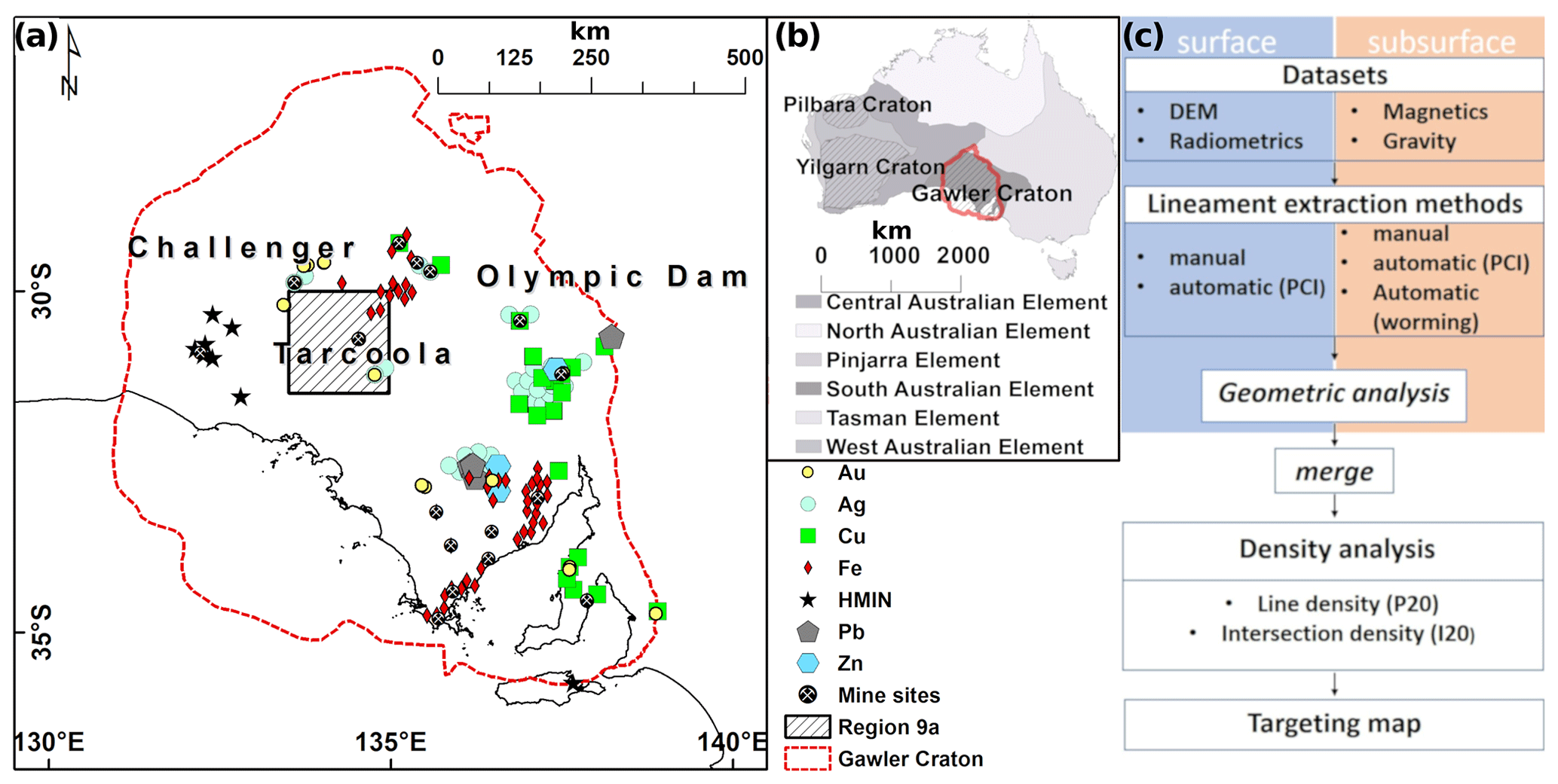
Figure 1(a) Economic mineral occurrences in the Gawler Craton. The mineral commodities include Au, Ag, Cu Fe, HMIN (heavy minerals), Pb, and Zn. (b) Overview map of the Australian continent showing the major crustal blocks and the locations of mineral-rich Archean to Proterozoic tectonic provinces. The Gawler Craton spans across nearly the entire South Australian Crustal element. (c) Outline of the workflow applied in this study to obtain targeting maps from surface and subsurface datasets. The first step is to categorise the datasets based on their penetration depth into surface and subsurface signals. Lineaments are then extracted with the methods outlined in Sect. 3.3, 3.4, and 3.5. Note that the multi-scale edge detection (“worming”) is only applied to the magnetic and gravity data, manual segmentation was only performed on the DEM, and automatic lineament mapping with the PCI Geomatica LINE module was applied to all datasets. We performed a geometric analysis on the extracted lineaments to highlight the variability between the different methods (Fig. 11). Targeting maps are derived from computed line density and intersection density maps. The first step for obtaining these maps is to merge lineaments into a single dataset if the lineaments are extracted with the same method. This is performed for surface and subsurface lineaments respectively, i.e. extracted from the DEM, and the radiometrics with the LINE module of the PCI Geomatica software are merged into a single dataset representing the collated lineaments attributed to changes in surface topology and chemical composition. A summary of the merged data utilised is shown in Table 1. The density maps are then computed for datasets that comprise surface and subsurface lineaments (see Table 2). We visualise the targeting maps as colour coded line density maps that are contoured by the intersection density. Based on a defined threshold, potential targeting areas are then highlighted in these maps. A more detailed workflow diagram is included in Fig. A1.
The bulk of the Paleo- to Mesoproterozoic rocks of the Gawler Craton enclose an Archean core in the central Gawler Craton with the oldest units being of Late Archean age (Reid et al., 2014). Internally, the Gawler Craton is subdivided into different domains based on contrasts in geophysical, structural, and geochemical characteristics (Ferris et al., 2002; Fairclough et al., 2003; Kositcin, 2010). The different rock units are often separated by crustal-scale shear zones that often coincide with the boundaries of the individual blocks. The region around Tarcoola includes four major provinces of the central Gawler Craton: the Christie, Wilgena, and Nuyts subdomains, and the Harris Greenstone belt (Fig. 2a).
2.1 Basement and cover sequence
The key geologic features that we seek to explore are structural and lithology discontinuities in the basement along with if and how they may relate to today's landscape and current topographic relief. In the following, we briefly describe the dominant lithologies in the study area from the oldest to the youngest unit and highlight the expected variability in aeromagnetic and gravity data.
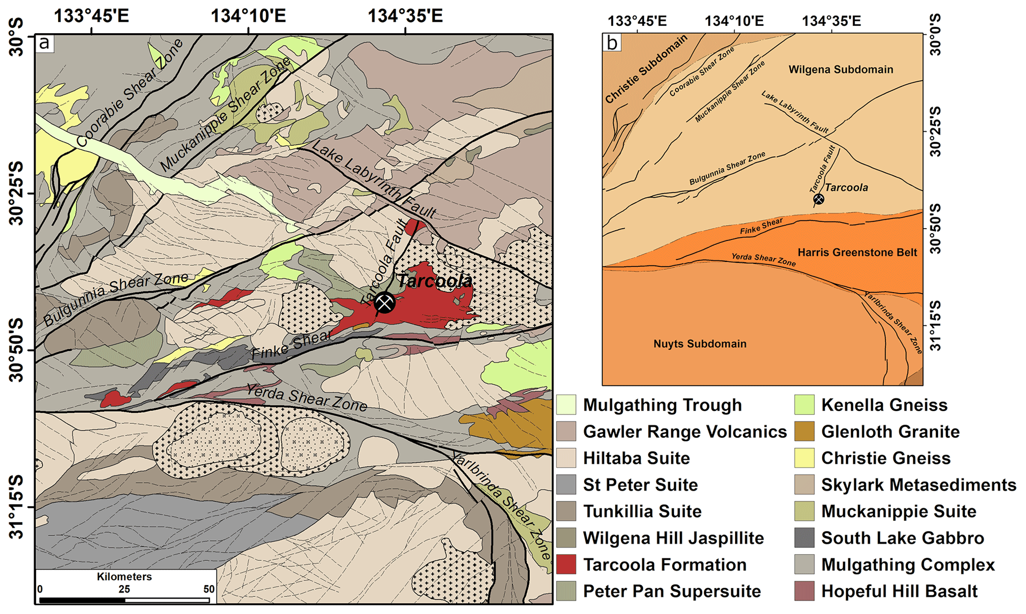
Figure 2(a) Structural interpretation of the subsurface based on magnetic, outcrops, and drill hole data (Pawley and Wilson, 2019). Large mylonitic shear zones cross the area dominantly in a SW–NE direction. Strong influence on feature extraction is expected from plutonic bodies and mylonite zones. Coorabie Shear Zone: CoSZ, Muckanippie Shear Zone: MuSZ, Lake Labyrinth Fault: LaLF, Yerda Shear Zone: YeSZ, Yarlbrinda Shear Zone: YaSZ, Finke Shear: FiS, Bulgunnia Shear Zone: BuSZ, Tarcoola Fault: TaF. (b) Structural domains of the study area. The boundaries of the domains often coincide with crustal-scale shear zones. The location within the Gawler Craton of the area shown in this figure is indicated in Fig. 1.
The interpreted Precambrian basement geology of the Harris Greenstone Belt comprises east-northeast-trending linear magnetic highs that often correlate with broad gravity signatures and are flanked by ovoid to elongated magnetic lows and highs (Hoatson et al., 2002). Rocks of the Harris Greenstone belt are found along the Flinke and Yerda Shear Zones and at the eastern margin in the central part of Fig. 2b.
Most rocks in the region are of igneous origin with only minor portions of metasediments. Rocks of the Mesoproterozoic Hiltaba Suite (see legend of Fig. 2) are prominent within the area of interest along with large plutons. The northeastern part of the study area was affected by the Gairdner Dyke Swarm at about 827 Ma that comprises predominantly northwest-trending dykes (Huang et al., 2015, and references therein). The youngest structure in the region is the Mulgathing Trough in the northwest that has an inferred Permian age.
The magnetic signatures could help to distinguish between different rock types as suggested by Hoatson et al. (2002), who showed that Archean granitic gneisses and granites are often irregular or elongated bodies with low-amplitude magnetic signatures, whereas Proterozoic granites comprise both zoned and massive ovoid plutons of low and high magnetisation. For the Hitaba Suite, Schmidt and Clark (2011) already pointed out the high variability in airborne magnetic signature.
Overlying the crystalline basement of the Gawler Craton in the analysed area are Palaeozoic, Mesozoic, and Cenozoic sedimentary sequences that combined form significant but variably thick cover ranging in thickness from 0 to more than 600 m. However, the spatial distribution of each sedimentary sequence is poorly understood (Hou, 2004).
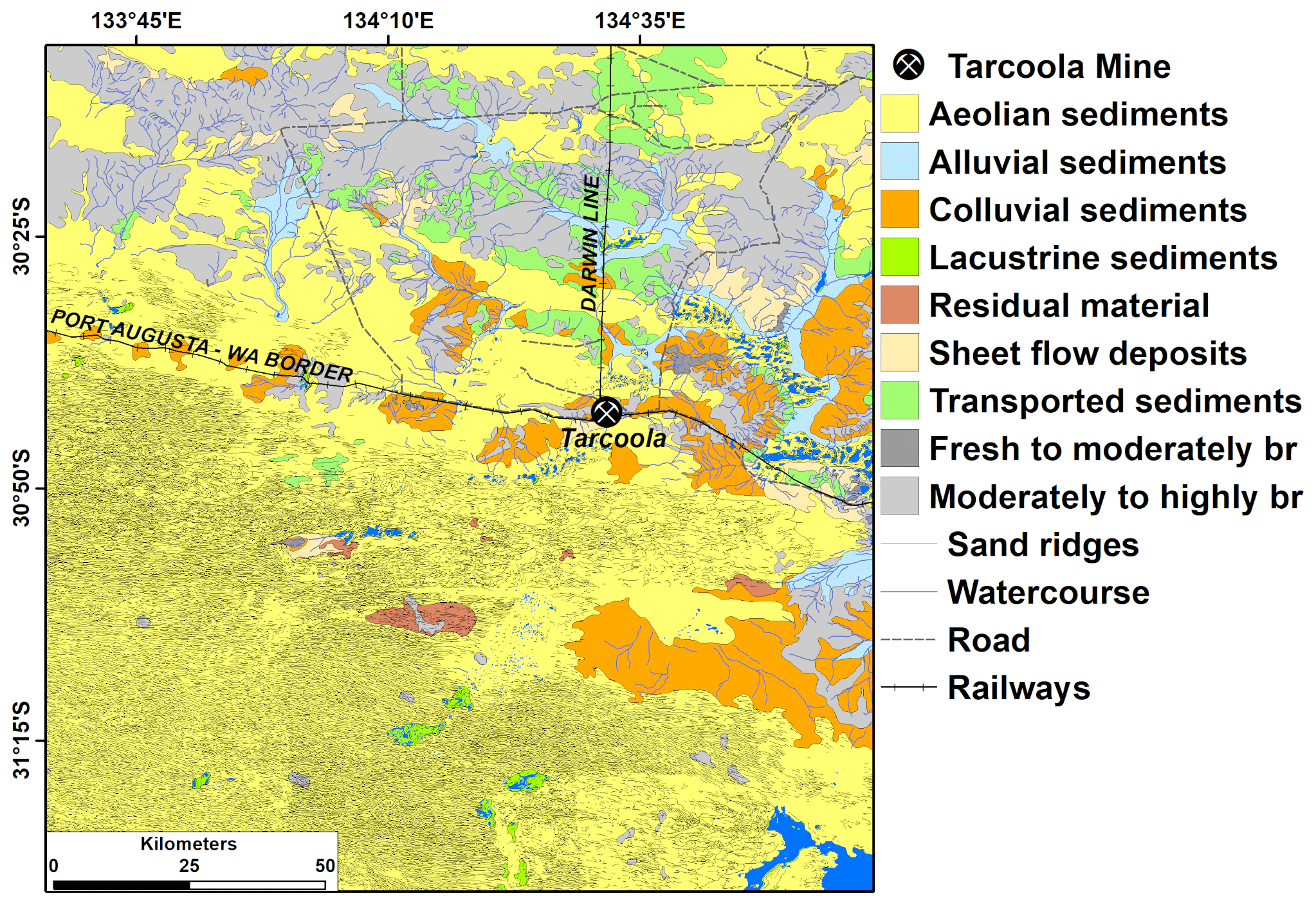
Figure 3Surface feature map displaying regolith material (Krapf et al., 2012), roads, watercourses, and sand ridges. Especially linear structures such as roads and sand ridges are expected to strongly influence the automated lineament extraction process. br: bedrock.
The terrain across most of the study area is relatively flat to moderately undulated. Prominent topographic highs are localised around dissected rocky outcrops. The surface is characterised either by aeolian sand covering variably weathered bedrock mainly in elevated parts of the landscape, or by saline playa lakes and drainage tracing topographic lows. One distinct feature is the longitudinal dune field that occupies an extensive area in the southwestern and southern part (Fig. 3) with individual plurikilometric-long dunes with W–E-trending crests.
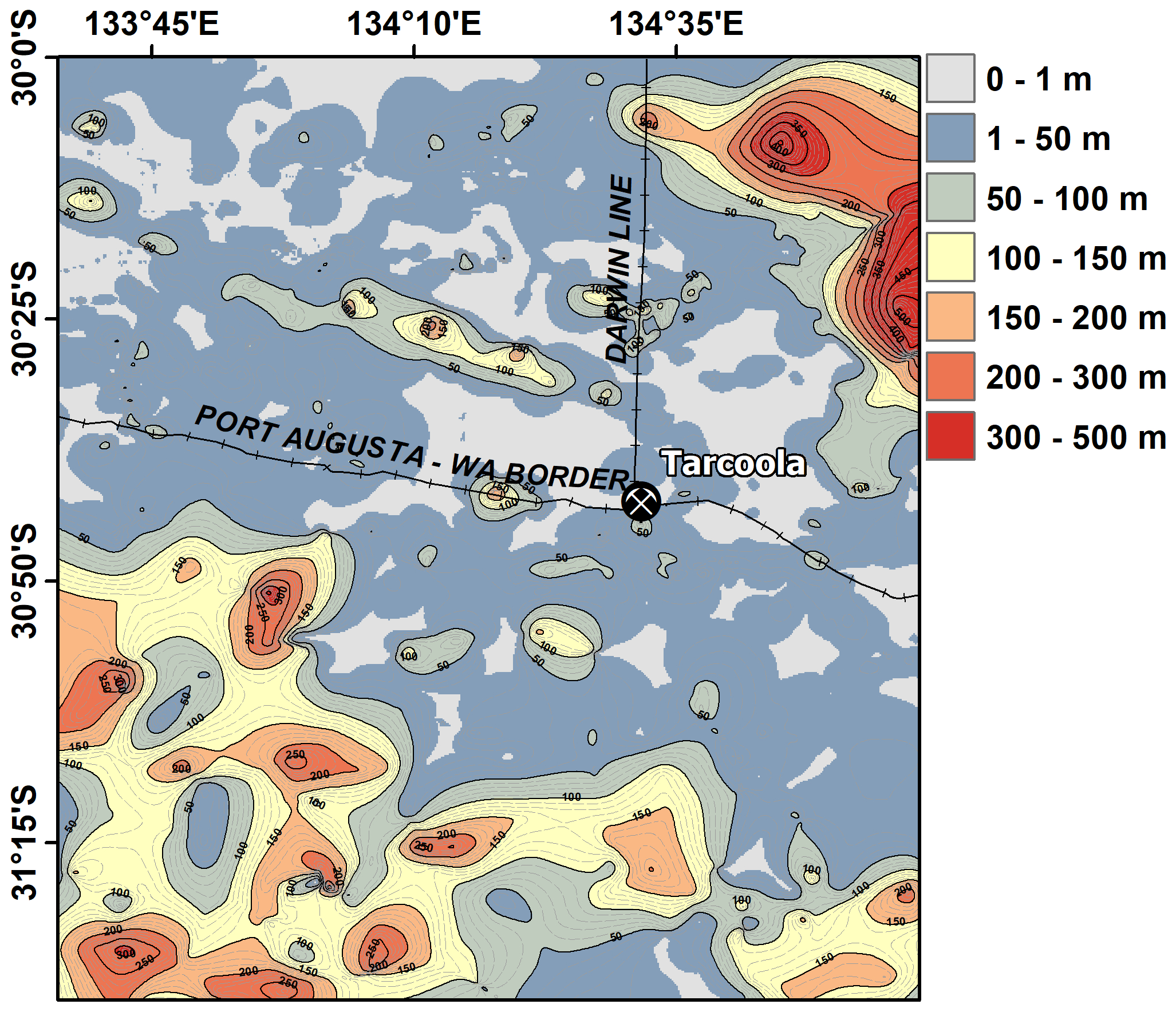
Figure 4Depth to basement map (Cowley et al., 2018).
The oldest preserved cover is composed of Late Carboniferous to Early Permian post-glacial sediments within the Mulgathing Trough in the northwestern corner of the study area (Fig. 2) (Nelson, 1976; Hibburt, 1995). Magnetic source depth analysis suggests that the trough is more than 600 m deep, with the maximum depths likely not detected (Foss et al., 2019). The overall variability of the cover thickness in the study region is shown in Fig. 4.
2.2 Structural framework
An interpretation of the geological framework was undertaken around Tarcoola (Wilson et al., 2018; Pawley and Wilson, 2019) using the new GCAS aeromagnetic data (see Fig. 5c) that were collected between 2017 and 2018, at 60 m ground clearance with 200 m spacing on east–west flight lines (Foss et al., 2019). The dominant linear structures that can be identified in the aeromagnetic data are shear zones and faults. Identified faults and shears tend to be relatively discrete zones whose magnetic signature was altered by circulating fluids, or by the juxtaposition of two blocks of rock with different magnetic characters. In general, the shear zones are prominent on aeromagnetic images as they form extensive structures that often separate lithological packages with contrasting magnetic characters or are associated with changing trends of the magnetic grain (e.g. Fig. 5c). Faults often form shorter, narrow features with changing magnetic expressions that can be difficult to recognise in rocks with a low magnetic response. For details on the signature of faults in aeromagnetic data we refer to Grauch and Hudson (2007). The area in Fig. 2 can be divided into a series of structural domains with distinct fault patterns.
Few faults are identified in the Christie Domain, although this could be due to the bland magnetically low character of the region. One exception is the >80 km long, northwest-trending Mulgathing Trough (Fig. 2b), which can be recognised as it is filled with Permian glacial sediments that affect its magnetic response.
The Wilgena Domain contains northwest-trending faults that are particularly prominent as narrow non-magnetic zones in the magnetic Hiltaba Granite plutons (Fig. 2b). Some faults are relatively straight to curvilinear and can be traced for more than 80 km (e.g. the Lake Labyrinth Fault), whereas others are shorter and form anastomosing and bifurcating structures. The northwest-trending faults typically show apparent dextral offset and usually cut the major shear zones. An exception to this trend is the north-northeast-trending Tarcoola Fault that appears to propagate from the southern Finke Shear Zone.
The faults form several patterns in the Nuyts Domain (Fig. 2). To the northwest, the faults are northwest-trending with dextral offset. The eastern Nuyts Domain is characterised by northeast-trending sinistral faults, aligned sub-parallel to the Koonibba Shear Zone located to the southwest of Fig. 2 (see detailed map of González-Álvarez et al., 2020). In the central Nuyts Domain, a pluton from the Hiltaba Suite has a long, straight northwest-trending margin that is bound by the Kooniba Shear Zone. The granite pluton adjacent to the shear is cut by abundant faults that are observed in several orientations and looks like a fracture zone. None of these faults extend across the Kooniba Shear Zone into the rocks of the St Peter Suite.
The NW- and NE-trending faults across a large portion of the study area cut the ≈1585 Ma Hiltaba Suite plutons. Therefore, the faults formed at or after ≈1585 Ma, likely during Kararan Orogeny that occurred either at 1570 Ma (Hand et al., 2007) or 1600–1570 Ma (Reid et al., 2017, and references therein). There is evidence that pre-existing structures (i.e. Gulgunnia, Muckanippie, and Coorabie shear zones (see Fig. 2) were reactivated during the Kararan Orogeny (Direen et al., 2005; Reid and Dutch, 2015). In conclusion, most of the large-scale fault zones could have provided pathways for mineralising fluids. Based on the observable offsets of pluton contacts a N–S-directed shortening can be assumed during the formation of the Au deposit mentioned above.
In the following section, we introduce the datasets used for lineament extraction and then describe the lineament analysis we employ to compare lineaments extracted by different techniques, followed by a description of the three lineament extraction techniques used.
3.1 Datasets
Lineaments extracted from a subset (region 9A (Childara)) of the Gawler Craton Airborne Survey (GCAS), the world's largest high-resolution airborne geophysical and terrain imaging program at 200 m line spacing, were analysed by Foss et al. (2019). The data that are released under the Creative Commons Attribution 4.0 International Licence include total magnetic intensity (TMI), radiometrics (RAD), and digital elevation model (DEM).
We utilised the DEM derived from laser altimeter subtracted from differential GPS heights (Fig. 5a), radiometric data (total dose) processed using the Noise Adjusted Singular Value Decomposition (NASVD) (Hovgaard and Grasty, 1997) (Fig. 5b), total magnetic intensity reduced to pole (Fig. 5c), and gravimetric data gridded to 100 m with a station spacing between 50 and 50 000 m (Fig. 5d).
The data presented are freely available through the South Australian Resources Information Geoserver (https://map.sarig.sa.gov.au/, last access: 5 January 2022).
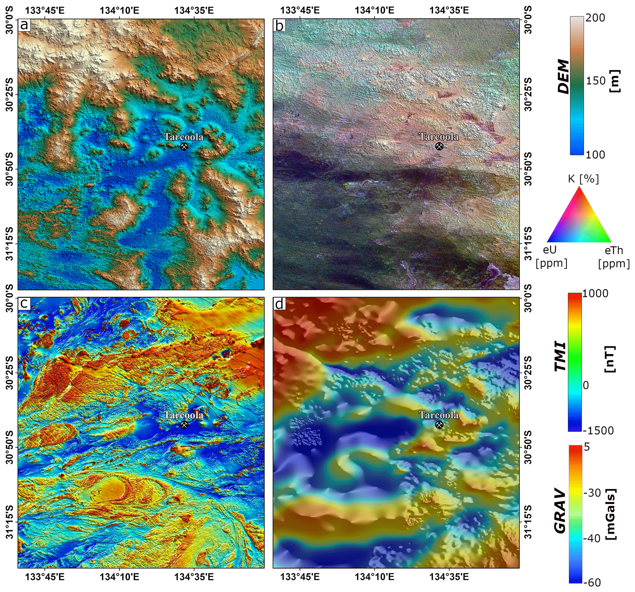
Figure 5(a) Colour digital elevation model (laser altimeter) (min: 84.08 m; max: 365.33 ), (b) colour radiometric dose rate (NASVD corrected) (min: 0.074 nGyh−1; max: 239.30 nGyh−1), (c) colour total magnetic intensity (reduced to pole) (min: −1978.16 nT; max: 21 638.8 nT), and (d) colour and hill-shaded Bouguer gravity anomaly image (Katona, 2017) (min: −158.15 mGal; max: 64.74 mGal). Data source: GCAS Region 9A, https://map.sarig.sa.gov.au/.
3.2 Lineament analysis
Lineament analysis allows for obtaining unbiased metrics for comparison of the data in terms of their dominant strike directions. For each dataset the principal orientations are automatically obtained. Assuming that the strikes represent a multimodal distribution, we first calculate the kernel density estimation (kde) using normal distributed kernels. The kde is a non-parametric estimator that basically smoothes each data point into a small density function based on the underlying kernel and bandwidth. The obtained kde function then represents the sum of all these subfunctions. By this we obtain an smoothed estimation of the distributions' probability density function. This analysis was performed using the FracG software (Kelka and Westerlund, 2021). For a general overview of how kde works we refer to Chen (2017).
For simplification, we assume that the individual principal strike directions follow Gaussian distributions. In this case, we obtain a best-fit model allowing for up to 10 principal strike directions (Gaussians) fitted to the obtained kde. The parameters of the Gaussians are obtained via maximum likelihood fitting. Goodness-of-fit testing is performed iteratively based on modified Akaike information criteria (Akaike, 1998). The amplitudes of the Gaussians are normalised and are proportional to the number of lineaments that belong to this distribution.
Figure 6 shows the principal orientations of the structural interpretation (Fig. 2a). Raw kernel density estimates are plotted as a dotted line to which the Gaussian model is fit. Clearly, two perpendicular directions dominate the data with a subordinate set of roughly N–S-striking lineaments.
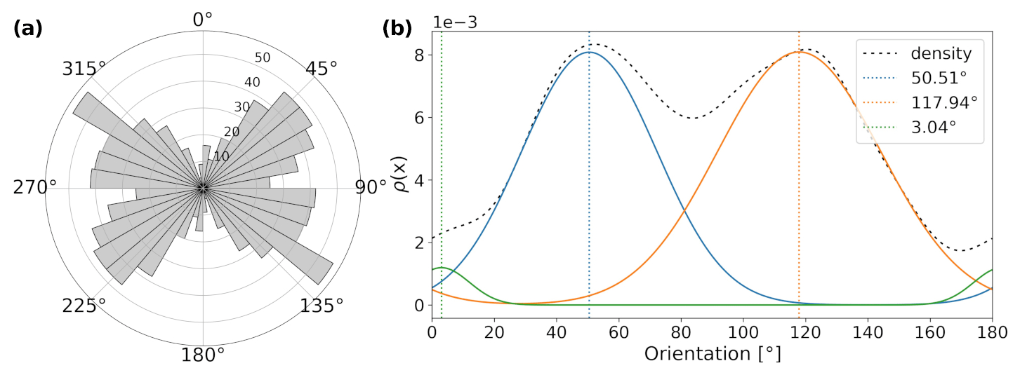
Figure 6Directional analysis of structural interpretation (Fig. 2a). (a) Rose diagram showing the distribution of strike directions of the structural interpretation with a bin size of 10∘. (b) Gaussian distributions fitted to the probability density function of the strike directions obtained via kernel density estimation.
3.3 Manual lineament extraction
Lineaments are pattern breaks within data that the human eye can depict as a straight or somewhat-curved feature in an image (Boucher, 1997). This is dependent on the person's visual ability as well as technical experience and hence mapping the presence and location of surface lineaments can vary significantly between individuals. By applying different types of preprocessing (e.g. edge detection filtering, hill shading etc.) different features in the raster image can be enhanced thus leading to different lineament sets segmented from the same dataset. Direct observation-based surface lineament mapping has been widely applied in geoscience and has been improved by the increasing availability of high-resolution satellite images as well as DEM and Multi-resolution Valley Bottom Flatness (MrVBF) (Gallant and Dowling, 2003).
Surface lineaments were manually mapped in the DEM (Fig. 5a) by direct visual identification and digitisation in ArcGIS 10.6. Figure 7 shows the manually mapped lineaments in the DEM (a) and in the raster representing the mean gradient component (b). The mean gradient component was calculated as the arithmetic mean of the horizontal and vertical gradient components obtained through Sobel convolution filtering. This edge detection filter can utilise different kernels for enhancing edges of different orientation (e.g. horizontal or vertical) (Shrivakshan and Chandrasekar, 2012). The mean gradient component we calculated as a preprocessing step prior to the manual segmentation contains enhanced edges in the horizontal and vertical orientation. The dominant orientation in both datasets is around 106 and 110∘, respectively. In both datasets, three Gaussians provide the best fit, whereas the two subordinate directions of both datasets differ significantly.
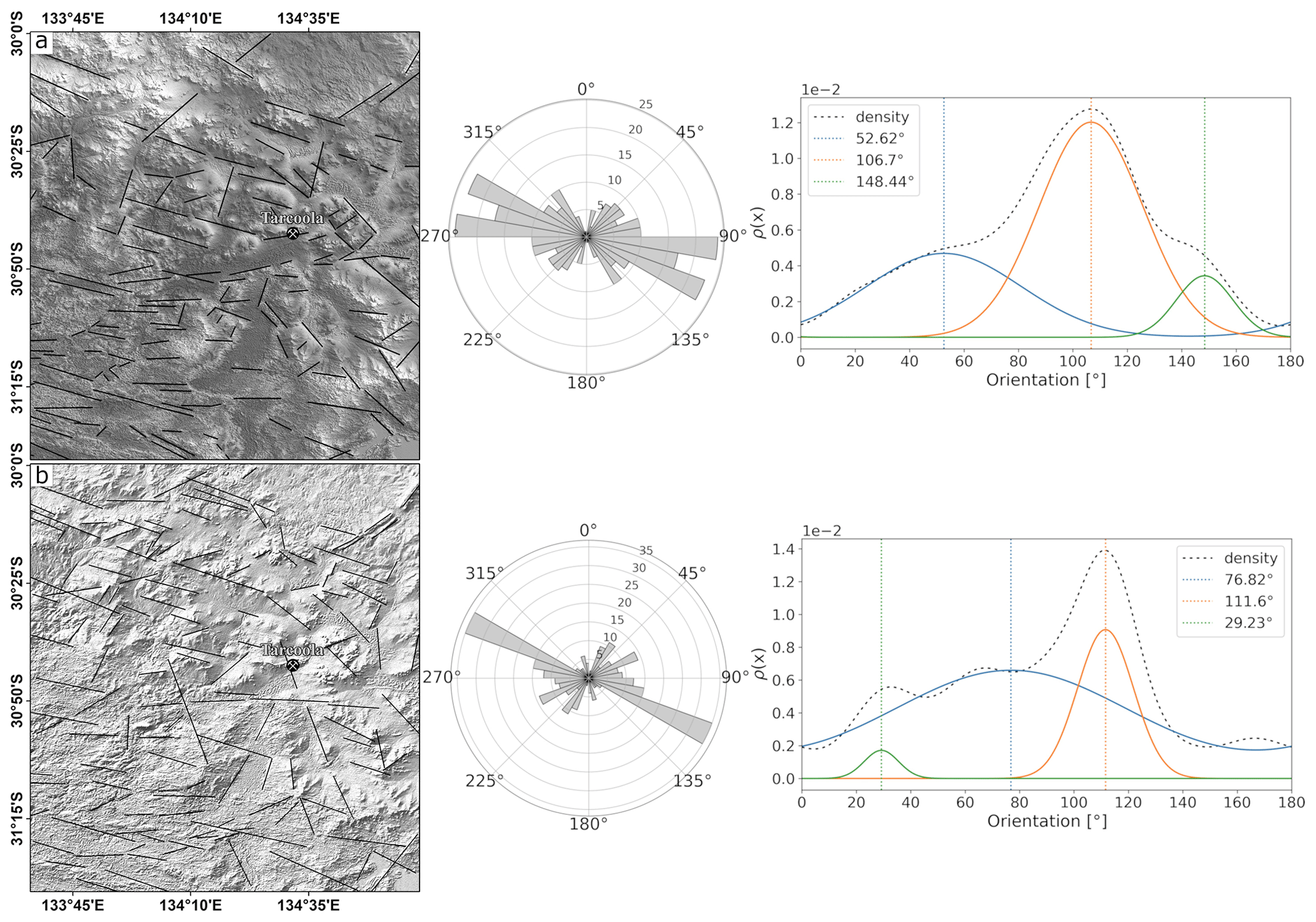
Figure 7(a) Manually segmented lineaments observed in the unprocessed laser altimeter DEM data. To the right of the map the rose diagram showing the distribution of strike directions (bin size of 10∘) and the Gaussian model fitted to the probability density function is shown. (b) Manually segmented lineaments obtained from the laser altimeter data after edge detection filtering. We show the mean horizontal and vertical gradient components obtained via Sobel convolution filtering. To the right of the map the rose diagram shows the distribution of orientation with a bin size of 10∘, and the lower plot represents the Gaussian models fitted to the probability density function.
3.4 Automatic gradient extraction (“worms”)
A multi-scale edge detection technique has been applied to the potential field data, which produces edge features called “multi-scale edges” (or colloquially “worms”). This technique (Hornby et al., 1999; Holden et al., 2000) relies on a wavelet transform based on the Green's function of vertical gravity or reduced-to-pole (RTP) total magnetic intensity. A low-resolution multi-scale edge mapping of the whole Gawler Craton was performed by Heath et al. (2009). Foss et al. (2019) applied a higher resolution mapping using the more recent GCAS Region 9A magnetic field data and updated gravity coverage. A fundamental part of this automatic edge detection technique is the upward continuation that acts similarly to a filter suppressing shallow sources (see Hornby et al., 1999, and Foss et al., 2019). In this contribution, we selected different heights of upward continuation for the gravity and magnetic data respectively in order to derive edge maps that comprise similar levels of detail of the subsurface. The reasoning behind our choice is on the one hand that gravity and magnetic field decay at different rates away from the source and on the other hand that the datasets we utilised have different resolutions. In order to derive lineament maps that comprise a comparable level of detail from the gravity and magnetic data we choose an upward continuation of 930 m for the gravity data and an upward continuation of 2070 m for the magnetic data. Note that these only represent a single example of the geophysical lineament ensembles computed and presented in Foss et al. (2019). In the framework of this study, where the potential field data were utilised to derive signal from the deeper subsurface, the two chosen datasets represent a good example for this automated lineament mapping technique.
The potential field data were processed using upward continuation (UC) to generate edge features that can be considered representative of different depths. Upward continuation suppresses high frequencies in the data and increases the weighting of signals from deeper physical property contrasts. Calculation of edge enhancement transforms at different upward continuation heights, producing a series of edge mappings (“multi-scale edges” or “worms”). Edges derived from the gravity data map subsurface density contrasts, and those from the magnetic field data map subsurface magnetisation contrasts. The edges (in particular the shallow edges) depend considerably on data distribution which is very regular for the magnetic field data, but highly irregular for the gravity data. In areas of sparse gravity coverage, it is not possible to map detail in the shallow gravity multi-scale edges. In compensation, the gravity field better expresses contributions from deeper property contrasts than the magnetic field. However, the principle value of having multi-scale edges derived from both gravity and magnetic field data is that they map quite separate physical properties, even though both properties depend on lithology. In some cases the contact between two lithologies is both a density and magnetisation contrast, and the two multi-scale edge vectors are strongly correlated, but in other cases a lithology contact may cause only a significant density contrast or only a significant magnetisation contrast, giving rise to edge vectors in only one of the fields. The combination of the two sets of edge vectors is therefore much more informative than either one alone. By their nature potential fields measured above a physical property interface are automatically smoother than the trace of that interface. They cannot include abrupt changes of trends, and at higher upward continuations the potential field and multi-scale edge expression of any straight-line property contrast becomes progressively more curved. There are therefore compromises in matching naturally curved multi-scale edges with corresponding straight lineaments extracted from the same dataset. The principal orientation of the lineaments is roughly E–W for the gravity and magnetic data (Fig. 8). The lineaments derived from the magnetic data (Fig. 8a) exhibit three main directions. In contrast, the strike of the gravity lineaments (Fig. 8b) are uniform with only one clear principal orientation.

Figure 8(a) Automatic gradient extraction with an upward continuation to 2070 m performed on the total magnetic intensity after pole reduction. To the right of the map the rose diagram shows strike distribution with a bin size of 10∘, and the Gaussian functions fitted to the probability density function are shown. (b) Automatic gradient extraction with upward continuation to 930 m for gravity data. To the right the rose diagram visualising the orientation distribution and the model fitted to the probability density function are shown. Upward continuation heights of the gravity and magnetic data were selected such that the lineaments represent similar detail.
3.5 Automatic lineament extraction
Lineaments have also been extracted from the DEM, radiometrics, gravity, and magnetics using PCI Geomatica's LINE function (Geomatics, 2005). This technique relies on properties inherent to the image (e.g. pixel intensity) making use of Canny edge detection (Shrivakshan and Chandrasekar, 2012) as the basis.
The gradient of an image is computed and pixels that are not a local maximum are suppressed. Edge strength threshold of pixels produces a binary image that, after applying a thinning algorithm, results in skeleton curves that represent edges. If a curve meets a minimum length criterion, the curve is approximated by line segments within an error threshold. Lineaments are the result of linking line segments if they have similar orientation.
PCI Geomatics defines a lineament as a “straight or somewhat-curved feature” (Geomatics, 2005), and the parameters control the extent to which edges detected in the image may result in a line feature. Originally intended to be used on radar images, the technique has been widely used in various remote sensing applications (e.g. Pandey and Sharma, 2019). Edges identified relate to significant changes within a given image and the resulting lineaments are highly dependent on user-specified parameters that control length and segment linkage. For a detailed description of the parameters used in this study we refer to González-Álvarez et al. (2020) and Pawley et al. (2021).
The lineaments were automatically extracted for datasets representative of surface (Fig. 9) and subsurface (Fig. 10) features. The surface data yield a single principal orientation of about 90 degrees in both lineament collections.
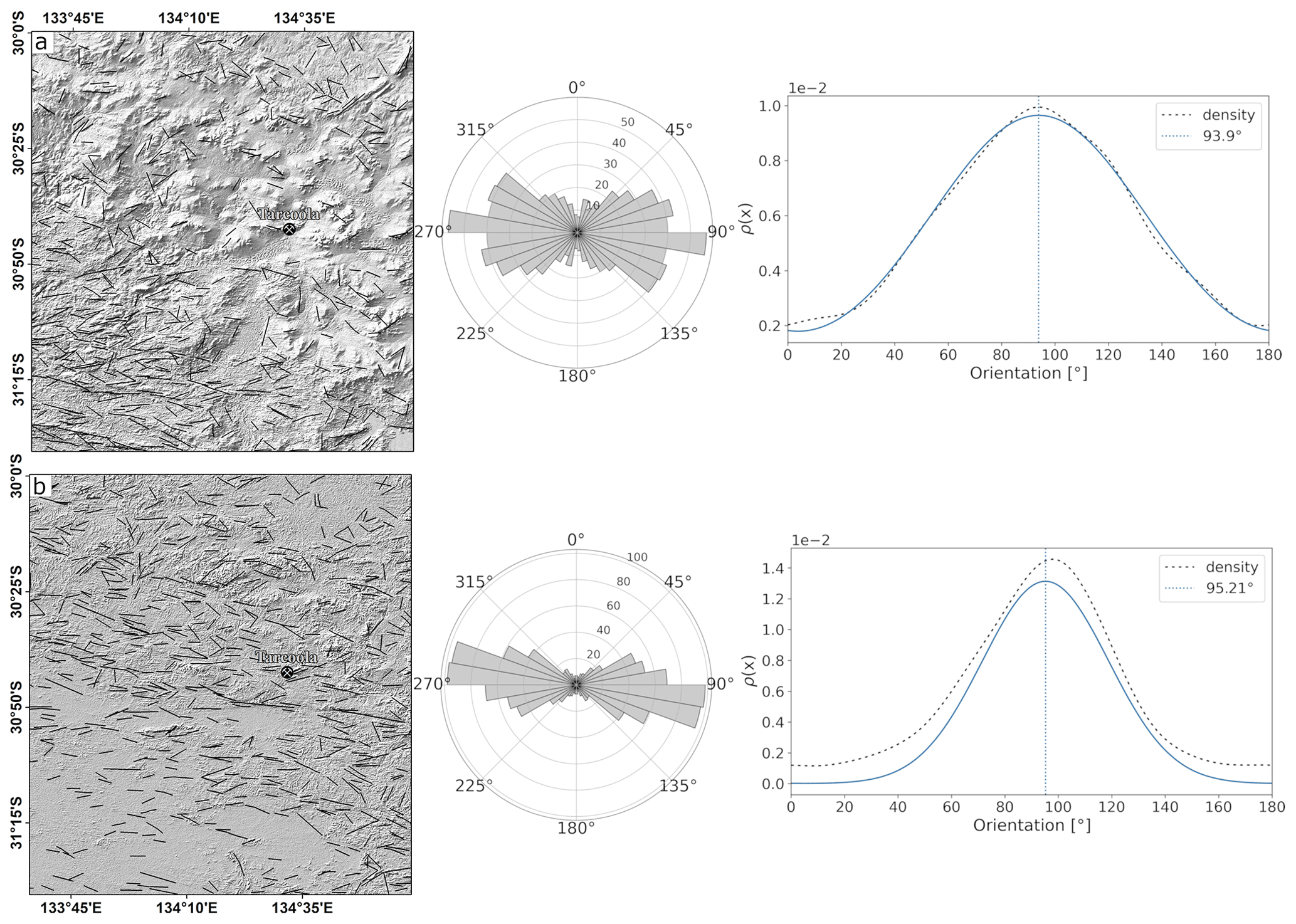
Figure 9Lineaments detected by PCI Geomatica’s LINE module in (a) the laser altimeter data and in (b) the radiometric data (total dose rate). The base map is the mean gradient component of the respective dataset used for visualisation purposes only. To the right the rose diagram and the models fitted to the probability density function are shown for each dataset (bin size of 10∘).
In contrast to the uniform distribution of lineament orientation obtained for the surface layers, the automatically detected subsurface lineaments exhibit two nearly equal principal directions for the total magnetic intensity (Fig. 10a) and a more uniform distribution obtained for the gravity data (Fig. 10b). The dominant directions in each subsurface dataset differ significantly and are oriented nearly perpendicular to each other.
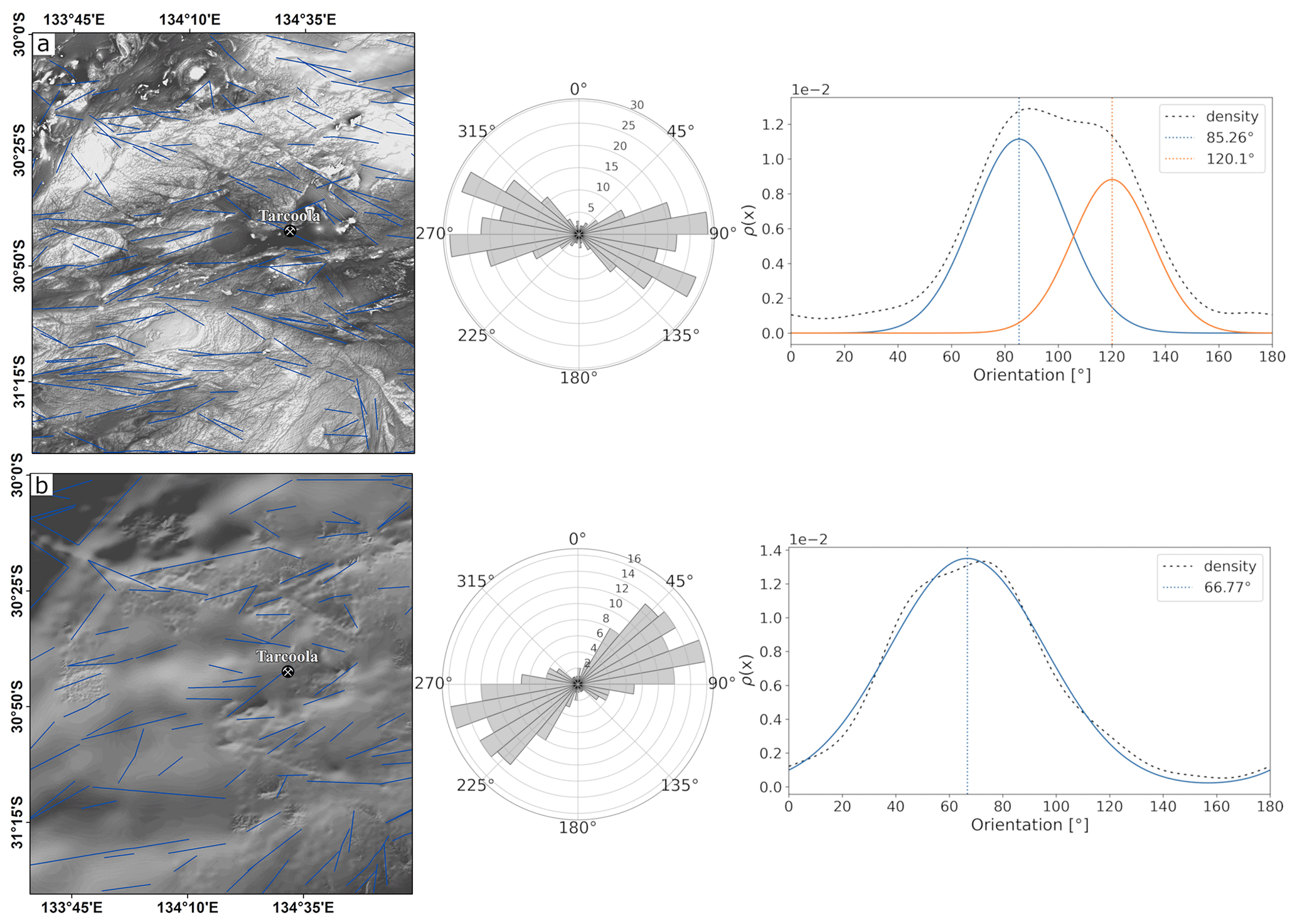
Figure 10Lineaments automatically extracted with PCI Geomatica LINE module from the total magnetic intensity (reduced to pole) (a) and the gridded gravity data (b). To the right of the maps the rose diagrams show the orientation distribution (bin size of 10∘) and the models fitted to the probability density of the empirical data.
The lineament datasets from the three techniques applied differ the most in terms of their length distribution (Fig. 11a). In particular, the automatically generated surface lineaments exhibit a narrow distribution with the highest density limited to regions around the mean and median. The length distributions of the lineaments automatically extracted from the subsurface data show a wider range slightly skewed towards smaller values. It is worth noting that the length tolerance of lineaments is an input parameter and the bias is well represented in the resulting lineament datasets. The automatic gradient extraction (worms) yields more distributed length of lineaments where smaller lineaments dominate the data. Manually extracted lineaments show a similar length distribution independent of whether the interpretation was performed on the processed or unprocessed elevation data. The structural interpretation that was performed mainly on the total magnetic intensity data exhibits the widest distribution. We note that the different techniques will yield variable results and different information can therefore be obtained from the same dataset by applying for instance the worming (Fig. 8) or automatic segmentation (Fig. 10). We do not seek to compare the geological or physical information inherent to each dataset but rather perform a statistical analysis to point out the most striking geometrical differences (e.g. length and orientation). An in-depth evaluation of which extraction methods yields more reliable or realistic geological information is beyond the scope of this study.
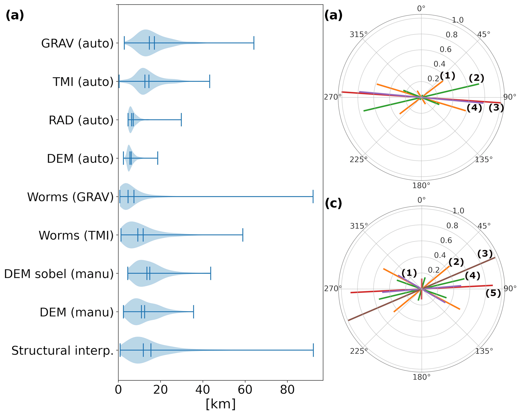
Figure 11(a) Violin plots showing kernel density estimates of the lineament length distributions. Minimum, maximum, mean, and median values are shown as vertical lines for each distribution. Plots were generated using the Python library at https://matplotlib.org/stable/gallery/statistics/violinplot.html (last access: 26 November 2021). (b) Principal orientations of surface datasets derived by fitting Gaussian distributions to the data (1: manual interpretation of laser altimeter; 2: manual interpretation of Sobel filtered laser altimeter; 3: automatic detection in laser altimeter data; 4: automatic detection in radiometric data (total dose count)). (c) Principal orientation of subsurface datasets obtained via fitting Gaussian distributions to the data (1: automatic detection in TMI; 2: structural interpretation; 3: automatic detection in gravity data; 4: TMI worms (UC 2070); 5: gravity worms (UC 930)). In both rose diagrams the length of the lines corresponds to the amplitude of their respective Gaussians.
The principal strikes exhibit a common E–W trend in the surface and subsurface datasets (Fig. 11a, b). The dominant orientations of the surface lineaments (Fig. 11b) scatter around the E–W plane with only one subordinate orientation that is somewhat oriented perpendicular (the line labelled 4: automatically extracted from radiometric data). The orientations of the subsurface lineaments are more diverse but also scatter mainly around the E–W plane. Subordinate orientations are more common in the subsurface lineament datasets and most pronounced in the worms (Fig. 8a, b) and in the lineaments automatically extracted from the total magnetic intensity (Fig. 10a). The latter exhibits a bimodal distribution that is comparable to the manual structural interpretation (Fig. 6). Overall, the automatically extracted surface lineaments tend to yield uniform distributions for length and orientation, whereas the automatically extracted subsurface lineaments exhibit wider length distributions and non-uniform strike directions. The automatic gradient extraction produces lineament sets with wider length distributions and orientations dominated by an E–W trend with subordinate orientations that are nearly perpendicular to the principal strike. Apart from the manual structural interpretation, this method is the only one presented in this study that produces strongly curved lineaments. Lineaments that are manually extracted show a comparable length distribution independent of whether the data were processed by edge detection filtering. The locations and orientations are influenced by the processing and so is the number of features (Fig. 7a, b). In summary, a dominant orientation trend is observable in the automatically generated surface and subsurface lineaments that is roughly east–west. Only the manually extracted surface lineament set shown in Fig. 7b and the structural interpretation (Fig. 6) exhibit considerable divergence from this orientation. The main difference between the different lineament sets is demonstrated by their length distributions (Fig. 10).
Here we present a workflow for exploration targeting based on lineament density and intersection density per unit area that utilises remotely sensed surface and subsurface data. Lineament datasets that are obtained with the same method and correspond to signals either both from the surface or both from the subsurface are merged (see Tables 1 and 2). The resulting dataset comprises the collated lineaments associated with topographical or chemical changes in the surface. We performed the same for the potential field data (gravity and magnetics) to obtain a collection of all geophysical lineaments detected by the respective extraction method. The aim of this analysis is to identify areas of maximum line and intersection densities in the combined surface and subsurface signals. The merged datasets with their name used in this section are shown in Table 1. The density maps are calculated for several combinations of surface and subsurface layers (Fig. 1c, Tables 1 and 2, and Fig. A1). The two types of density maps for deriving potential exploration targets are as follows:
-
density maps of lineaments per area (P20) and
-
density maps of lineament intersections per area (I20).
P20 maps represent the number of lineaments per unit area derived for rectangular sampling windows of size 2 km by 2 km. The pixel resolution of the derived raster file is set to the search window size. I20 maps are derived by converting the lineament data into a graph representation where intersections between lineaments are vertices (Sanderson et al., 2019). The number of intersections is derived using a pixel size of 2 km by 2 km and circular sampling windows with a radius of 2.5 km. The maps are then up-sampled via bilinear interpolation to a cell size of 500 m by 500 m. To obtain the density maps we used the open-source software FracG (Kelka and Westerlund, 2021).
The targeting maps are derived by overlaying the P20 maps with contours of the I20 maps (Figs. 12, 13, and 14). We used combined lineament data that represent surface or subsurface signals (see Table 1). In cases where we utilised the structural interpretation (Fig. 2) as the subsurface datasets the density maps comprise three individual lineament datasets (Figs. 12 and 13a), whereas the other targeting maps are comprised of four lineament sets (Figs. 13 d and 14). The reason behind this is that the remotely sensed data comprise two datasets for the surface (DEM and radiometrics) and two datasets representing subsurface (TMI and gravity). Furthermore, the signals might detect features at different scales whereby the sensitivity for structures at a particular scale is a function of penetration depth and spatial resolution. In particular, the gravity and magnetic data used in this study have very different resolution (Fig. 5) and will therefore yield lineament maps with different levels of detail. Datasets used for obtaining the respective targeting map and extraction methods used for obtaining the utilised lineaments are summarised in Table 2. We further classified the targeting maps into “manual”, “automatic”, or “semiautomatic” indicating whether the underlying lineament sets were derived with purely manual segmentation, represent a combination of manual and automatic extraction, or are obtained solely by automatic segmentation (Table 2).
Considering not only the overall lineament density but also the intersection density allows us to further constrain potential targeting areas. By obtaining intersection densities, cross-strike features can be identified that are thought to represent zones of enhanced permeability (Wheeler, 1980; Southworth, 1985). Areas of enhanced structural complexity or numbers of cross-strike discontinuities could therefore represent zones for preferential upwelling of mineralising fluids. We suggest that the adjacent areas that comprise an overall high density of lineaments represent preferential exploration targets. For identifying these mineral potential zones, we set a threshold of 9 intersections per 500 m by 500 m pixel size and then visually identified the areas of overall high densities in the vicinity of these specific points as favourable targeting areas. The threshold is kept constant across datasets in this study to ensure a better comparability but would need to be adjusted depending on the underlying data for more reliable targeting.
Table 1Merged datasets corresponding to surface and subsurface signals obtained with the same method.
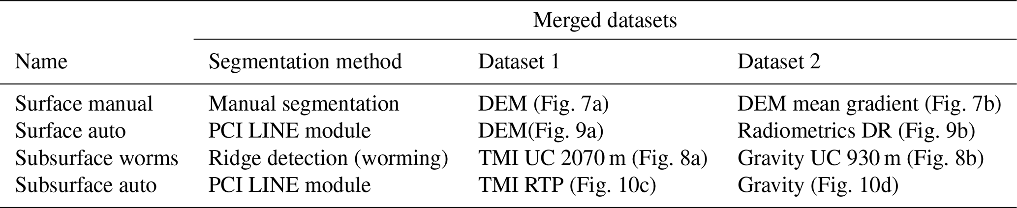

Figure 12(a) Targeting map derived from “surface manual” combined with the structural interpretation (Fig. 2a). (b) Lineament density map (P20). (c) Intersection density map (I20). Potential targeting areas are indicated by red ellipses.
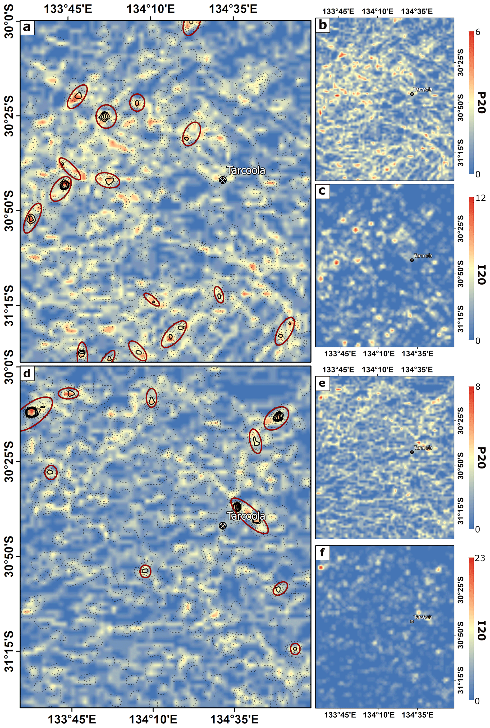
Figure 13(a) Targeting map derived from “surface auto” and the structural interpretation. (b) Lineament density map (P20). (c) Intersection density map (I20). (d) Targeting map derived from “surface manual” and the “subsurface worm”. (e) Lineament density map (P20). (f) Intersection density map (I20). Potential targeting areas are indicated by red ellipses.
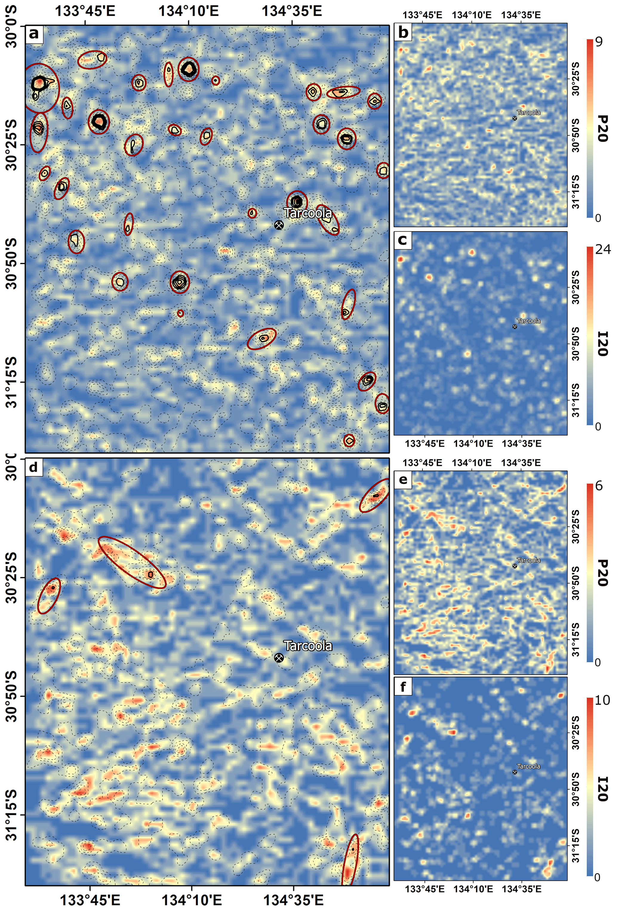
Figure 14(a) Targeting map derived from “surface auto” and the “subsurface worms”. (b) Lineament density map (P20). (c) Intersection density map (I20). (d) Targeting map derived from “surface auto” and the “subsurface auto”. (e) Lineament density map (P20). (f) Intersection density map (I20). Potential targeting areas that are located at the margins of the domain are indicated by red ellipses.
Table 2Summary of the targeting datasets (Figs. 12, 13, and 14) and name convention used in the combined targeting map (Fig. 15).
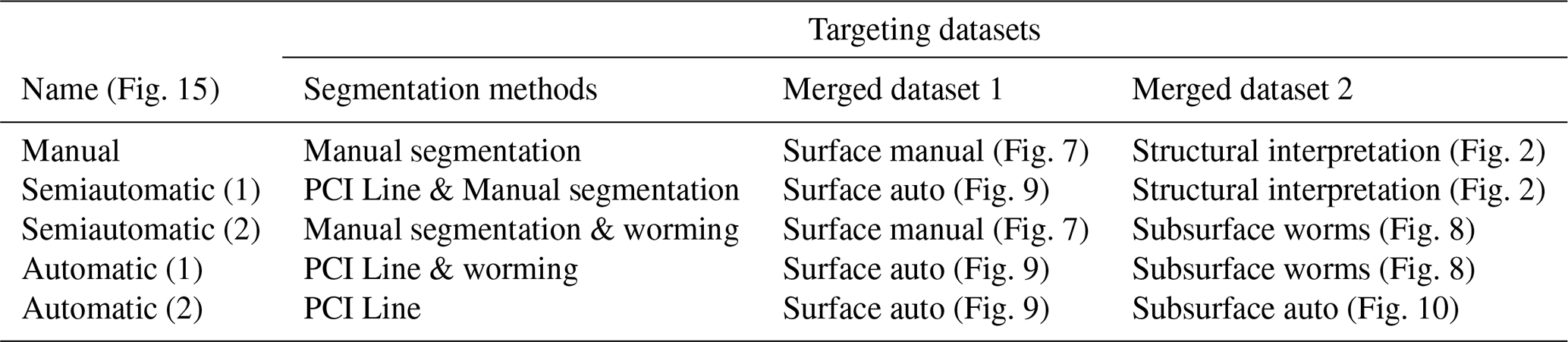
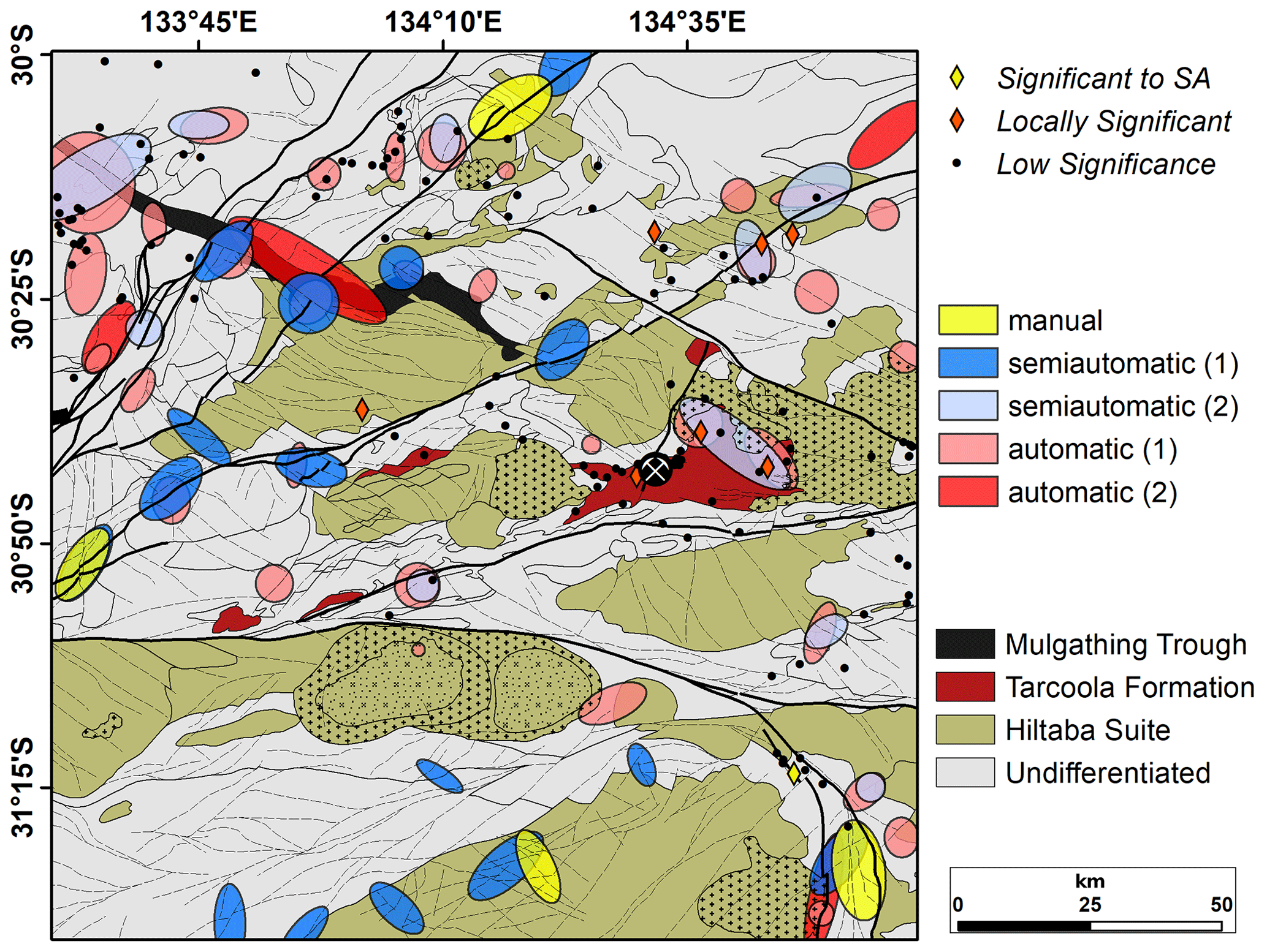
Figure 15Target areas identified by different combinations of lineament sets displayed on a geological and structural map. In the legend manual refers to datasets that are divided solely through expert interpretation (Fig. 12), semiautomatic represents datasets that are a combination of manually interpreted data (Fig. 13), and automatic refers fully automatically extracted lineament data (Fig. 14). Yellow and red diamonds indicate state-wide (SA: South Australia) and locally significant mineral occurrences that were detected in drill cores. The black dots are mineralisations that are below economic significance. The legend for the geological and structural units is shown in Fig. 2a.
This is the first study to utilise the newly acquired high-resolution datasets of South Australia (GCAS Region 9A (Childara)) to investigate the applicability of lineament mapping and extraction from a variety of datasets as a potential exploration tool. As both manual and automatic lineament extraction methods are subject to bias, we first compared the results obtained from both approaches.
During manual interpretation bias arises from subjectivity that is introduced by different interpreters (Raghavan et al., 1993) and can also be caused by scale or variable processing techniques for edge enhancement such as illumination azimuth (Scheiber et al., 2015; Masoud and Koike, 2017). We do not seek to explore these aspects but do note that interpretation bias may be playing a role in creation of the manual lineament datasets used. Automatic mapping methods can also be subject to bias related to the type of applied edge detection filter and underlying segmentation algorithm. We applied the lineament extraction algorithm from the commercial software PCI Geomatica, as one of the main topics of this study is comparing different conventional methods with automatic detection methods. Some input parameters of the PCI Geomaticas LINE module will certainly introduce a bias towards certain length distributions of the extracted lineaments. The two most important parameters are the threshold to length and the threshold to angular difference that defines the maximum difference in orientations for uniting two segments (see Table 7 in Kelka and Martinez, 2020, for details on the parameters). We note that recently several new approaches were suggested for automatic lineament mapping (e.g. Zhang et al., 2006; Hashim et al., 2013; Mohammadpour et al., 2020; Xu et al., 2020) and utilising one of these might yield results different to the ones presented here.
We will first discuss the similarities and differences of the surface and subsurface lineament sets obtained with the different methods pointing out the individual strength or weaknesses. Lineaments obtained by manual mapping in this study scatter around a particular length (Fig. 11). The length distribution of automatically extracted surface lineaments is even narrower, pointing towards a bias in lineament detection potentially related to the parameter combination applied for automatic mapping (see Sect. 3.5). One other major difference is that the manual mappings yield three main directions for each dataset, whereas the automatic detection exhibits uniform distributions. The principal orientation of automatically and manually extracted lineaments are similar for the radiometrics and DEM, respectively, but differ by a maximum of 18∘ between the methods when compared to the dominant directions obtained from the manually derived lineaments.
The automatic detection method yields data that are more representative for local-scale geomorphological features visible by the strong influence of the sand ridges in the southwestern part. In contrast, a human interpreter tends to identify the general trends in the data where results can be biased by the preprocessing of the data such as edge enhancement filtering. In summary, a general trend of superficial features extracted automatically and manually scatter around a E–W to NNW–SSE direction, and therefore this orientation is likely a characteristic regional feature of the cover across the investigated area. Whether automatic lineament extraction is superior to manual mapping cannot be stated with certainty based on the data presented in this study. Choosing one method over the other might depend on the type and the thickness of cover. Generally human investigators identify more regional trends, which are probably hard to detect automatically. The reason behind this is that a human interpreter will consciously detect the trends of lineaments and will merge them even if there are large gaps between the identified edges.
Geophysical lineaments are obtained from the gravity and magnetic data via automatic gradient extraction. The lineaments obtained from each geophysical dataset differ significantly in terms of length distribution and principal orientation (Fig. 8). This could be attributed to different depths the upward continuation represent but is more likely to reflect the difference in resolution of the data and the physical properties each dataset is sensitive to. The gravity data yield lineaments that are attributed to major lithological boundaries pronounced by density contrasts. In the study region the prominent boundaries are the margins of the domains that often coincide with large crustal-scale shears and the Mulgathing Trough in the northwest (see Fig. 2a, b). While the major crustal-scale elements are traced by the lineaments extracted from the gravity data, the lineaments obtained from the magnetic data seem to reveal a more detailed picture of the subsurface structural framework. In addition to domain boundaries the magnetic lineaments also outline large intrusive bodies. In line with the structural interpretation, three main directions are detectable for the magnetic worms (Figs. 2 and 6) but only two for the gravity worms (Fig. 8). While the edge vector's orientation and length distributions differ significantly, a reasonable correlation considering their locations is observable (Fig. 8). In line with Foss et al. (2019), this suggests that the mapping of gravity and magnetic contrasts with worms allows for correlating the magnetic and gravity field anomalies. It must be pointed out that the mapped edges only act as approximate markers of the horizontal contrasts in density or magnetisation (Foss et al., 2019). We note that utilising different values for the upward continuation will yield lineament maps comprising different levels of detail, and the datasets shown in this study represent only a single example from the range of upward continuations used in Foss et al. (2019). We note that using different values will alter the results and represents a source of uncertainty. However, for the purpose of this study the two upward continuation values were chosen to allow a more reliable comparison between the different datasets.
The presence of magnetic remanence may alter the field anomaly, rendering the reduction-to-pole data we used less useful. However, for our purposes of extracting lineaments from multiple datasets, the uncertainty in the degree of magnetic remanence is of less concern compared to the uncertainty associated with the different automated and manual techniques in extracting lineaments. We note that the magnetic and gravity datasets are of different resolution and in particular the resolution of the gravity dataset is non-uniform. As the upward continuation acts similar to a low-pass filter the difference in resolution becomes negligible allowing for a more reliable comparison of the potential field data used in this study.
Automatic lineament mapping performed with PCI Geomatica (Geomatics, 2005) yields a picture less consistent with the structural interpretation of the subsurface framework. While the automatically extracted gravity lineaments still outline some crustal-scale boundaries (especially evident for the graben structure in the northwest) the information associated with the automatically extracted geophysical lineaments is inferior compared to the information that can be obtained by automatic gradient extraction, and the latter method should be favoured for the mapping of geophysical lineaments. The worms trace the subsurface in greater detail, and profound physical meaning can easily be attributed to the location of the lineaments as they are associated with strong lithology contrasts within the basement units. In contrast, the automatically extracted lineaments pick up a rough impression of the structural framework of the subsurface with only major elements detectable in the data, such as major shear zones and the Permian graben. We conclude that automatic gradient extraction is the superior technique for extracting geophysical lineaments from high-resolution magnetic data and from gravity data with variable resolution.
In Sect. 5 we tested an approach that integrates surface and subsurface lineaments in a simple framework for exploration targeting that is based on identifying areas of high lineament density and high intersection density. The justification for this approach is that welling of hydrothermal fluids is often associated with structurally complex zones that comprise a high intersection density (e.g. Dimmen et al., 2017). Areas comprising an overall high density of discontinuities that are adjacent to such zones of high structural complexity represent preferential exploration targets for hydrothermal mineralisation. By combining surface and subsurface datasets we not only account for intersections in subsurface datasets but also for intersection of subsurface and surface lineaments. Such cross-strike discontinuities are an additional indicator for structurally complex zones and are taken into account in our workflow.
Figure 15 shows the target areas identified by the different methods. At the current stage the areas identified as potential targets by different methods represent the most promising regions for follow-up hydrogeochemical sampling for identifying mineral footprints in the cover. These are probably northeast of the Tarcoola mining site at the margins of a large intrusive body, in the northwestern part where the edge of Permian graben is cross-cutting the Muckamippie Shear Zone, the region in the southeast close to the Yarlbrinda Shear zone, and the area in the northeast where mineral occurrences are reported along the Bulgunnia Shear Zone. Most of the targeting areas are located along the shear zones that form the borders of the geotectonic provinces. Giving that the area is part of the central Gawler gold province where mineralisation is mainly shear-hosted Au (Hand et al., 2007, and references therein) this seems to be in line with the existing knowledge of the region. In addition, the targeting areas are often associated with the margins of the Hiltaba Suite (in particular in the southern part of Fig. 15). Here it is important to note that the gold deposits in the central Gawler Craton exhibit some similar characteristics considering the mineralisation style, as the gold is dominantly hosted in sulfide-poor structurally controlled quartz veins that seem to be spatially related to the Hiltabas Suite (Daly, 1993). We do not directly identify the deposit exploited at the Tarcoola mine but an area to the northeast that is situated along the margin of the Tarcoola formation (known host-rock Pawley and Wilson, 2019) that includes two mineral occurrences of local significance.
Uncertainty in manual lineament mapping is directly related to the person's experience and the scale they are intending on mapping. The manual extraction of lineaments in this study focused on the regional linear trends (lineament greater than 1 km). Addressing uncertainty for the automatic lineament mapping is difficult and directly related to the resolution of the underlying datasets. In case of the automatic gradient extraction, the upward continuation can pose another source of uncertainty related to the loss of detail that increases with higher upward continuations. For an example of how uncertainty in lineament mapping can be assessed statistically, we refer to Pawley et al. (2021). For a reliable interpretation of the obtained lineament maps the geological history of the respective area must be considered. This means that differently oriented lineament sets could correspond to different tectonic and fluid flow events. In areas comprising multiphase deformation some extracted lineaments might therefore not be of relevance for the targeted mineral system and, for instance, directional constraints on the utilised lineaments would need to be applied. In the case study presented here, the youngest orogenic event (Kararan Orogeny) is thought to be linked to the mineralisation (Fraser et al., 2007; Bockmann et al., 2019) and to the reactivation of pre-existing structures (Direen et al., 2005; Reid and Dutch, 2015). In this special case there is no need for applying strict constraints on the extracted lineament sets, but this might be necessary for other regions.
We note that relatively little known mineralisation coincides with the targets identified by the lineament analysis (Fig. 15) and further research is needed to validate the reliability of the presented workflow. Geological knowledge of the area might help to reduce the number of false positives obtained by lineament-based exploration targeting.
In this study we pointed out the differences between subsurface and surface lineaments in the Gawler Craton in South Australia mapped or extracted with different methods and from a variety of remotely sensed and geophysical data. We determined the principal orientations of each dataset by automatically deriving a best-fit Gaussian model of the data. Overall an E–W direction dominates in surface and subsurface datasets that likely represent the structural grain of the area. Surface lineaments manually mapped are clearly subjective and can be biased due to preprocessing of the data. Compared to automatic extraction the main difference seems to be the scale on which the extracted lineaments play a role; the manual interpretation picks up regional-scale trends, whereas automatically extracted features represent smaller-scale, locally relevant structures. We found that the automatic gradient extraction (“worming”) is superior to automatic lineament extraction performed with PCI Geomatica as the worms detect more details that are related to lithological and structural contrast. In this study we showed that automatic gradient extraction yields geophysical lineaments associated with a profound geological meaning compared to automatically detected edges. In terms of the surface lineaments we conclude that the automatic extraction represents a method that picks up more local-scale features and is likely well suited for well exposed areas. However, in areas that comprise a thick, reworked cover manual mapping of lineaments yields a more regional-scale picture and seems to represent a reliable method.
An integrated workflow that utilises surface and subsurface lineaments should include density per unit area and intersection density per unit area. We found that a combination of geophysical lineaments derived by automatic gradient extraction combined with either manually or automatically mapped surface lineaments represents the most promising combination of data for exploration targeting. The gravity and magnetic worms will coincide with present lithological boundaries or major structural features. To clearly state whether edges or lineaments observable in the surface data are correlated with crustal-scale features such as shear zones requires further research. For efficiently combining intersection density and line density for targeting, spatial clustering algorithms might yield more reliable results compared to the simple approach presented in this study. The crucial parameters will be setting an appropriate threshold for intersection and line density for determining target areas.
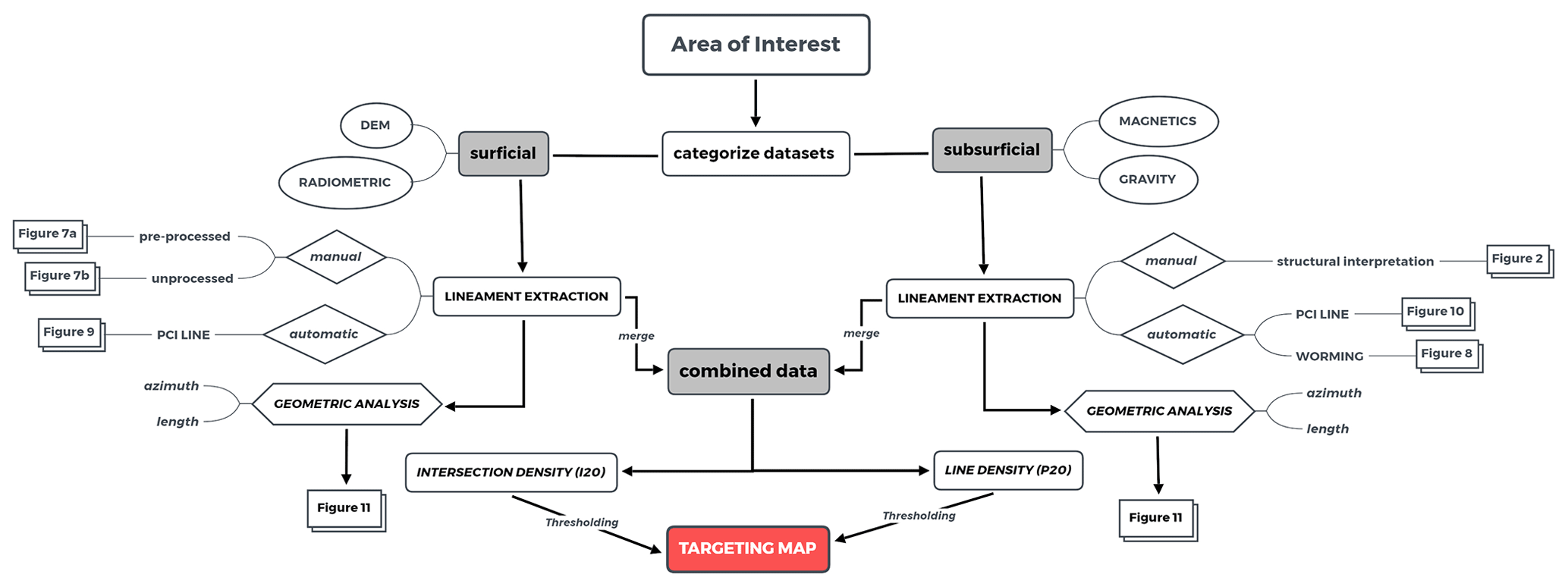
Figure A1Detailed sketch of the workflow we followed in this study. To generate targeting maps, lineament maps derived from surface (DEM and radiometrics) and subsurface data (magnetics and gravity) are generated. We utilise different automated and manual methods to obtain these maps as outlined in Sect. 3. As part of this contribution, a geometric analysis is performed on each individual lineament set to highlight the variability in principal orientation and length. Lineaments representing superficial or subsurface features are merged if they are obtained with same extraction method (see Table 1). In the subsequent step, the combined data (see Table 2) are used to compute line density and intersection density. The targeting maps are then derived by applying a user-defined threshold in order to highlight the regions of interest. Note that in this publication we applied an uniform threshold to all datasets. In essence, the workflow comprises five subsequent steps: (1) categorise the data, (2) extract the lineaments, (3) combine surface and subsurface lineaments that are segmented by the same method but are derived from different data, (4) merge surface and subsurface lineament datasets into a combined dataset, and (5) compute density maps highlighting the regions of interest based on a defined threshold.
The datasets and the code for automatic lineament analysis are freely available:
-
South Australian Resources Information Gateway – https://sarigbasis.pir.sa.gov.au/WebtopEw/ws/samref/sarig1/wci/Record?r=0&m=1&w=catno=2039795 (data) (Katona et al., 2018)
-
FracG – http://hdl.handle.net/102.100.100/421301?index=1 (code) (Kelka and Westerlund, 2021).
UK wrote the paper with input from all authors, analysed the data, and developed the computational framework. CM wrote parts of the paper, analysed data, performed the automatic extraction of lineaments, and revised the paper. CK devised the project, wrote parts of the paper, performed the manual lineaments extraction, and revised the paper. SW developed the computational framework, helped with data visualisation, and revised the paper. IGA devised the project, helped with data interpretation, and revised the paper. MP wrote parts of the paper, performed the structural interpretation, helped with data interpretation, and revised the paper. CF performed the automatic gradient extraction for the geophysical datasets, helped with interpretation, and revised the paper.
The contact author has declared that neither they nor their co-authors have any competing interests.
Publisher’s note: Copernicus Publications remains neutral with regard to jurisdictional claims in published maps and institutional affiliations.
This article is part of the special issue “State of the art in mineral exploration”. It is a result of the EGU General Assembly 2020, 3–8 May 2020.
The work performed is with support from the Geological Survey of South Australia, and the provision of high-resolution airborne geophysical and terrain data for Region 9A from the Gawler Craton Airborne Survey (GCAS) by Laz Katona and Jonathan Irvine. Carmen Krapf and Mark Pawley publish with the permission of the Director of the Geological Survey of South Australia.
We thank the leadership team of the CSIRO Deep Earth Imaging Future Science Platform for supporting this collaboration with CSIRO's Mineral Resources Business Unit.
We thank Nicolas Beaudoin and the four anonymous reviewers for their thorough revision which helped to improve this paper.
This paper was edited by Alba Gil de la Iglesia and reviewed by Nicolas Beaudoin and four anonymous referees.
Akaike, H.: Information theory and an extension of the maximum likelihood principle, in: Selected papers of Hirotugu Akaike, pp. 199–213, Springer, 1998. a
Bockmann, M., Wilson, T., Pawley, M., Payne, J., and Dutch, R.: LA–ICP–MS geochronology from the Tarcoola Goldfield region, 2018–2019, Report Book 2019/00015, 2019. a, b
Boucher, R.: Lineament Tectonic Data, South Australia, with a Focus on the Cooper Basin, Report Book 97/39, Department of Mines and Energy Resources South Australia, 1997. a, b
Budd, A. and Fraser, G.: Geological relationships and 40Ar/39Ar age constraints on gold mineralisation at Tarcoola, central Gawler gold province, South Australia, Aust. J. Earth Sci., 51, 685–699, 2004. a, b
Chen, Y.-C.: A tutorial on kernel density estimation and recent advances, Biostat. Epidemiol., 1, 161–187, 2017. a
Cowley, W., Katona, L., Gouthas, G., Hough, L., Menpes, S., and Foss, C.: Depth to crystalline basement data package: South Australia, Geoscience Data Package [data set], 3, https://sarigbasis.pir.sa.gov.au/WebtopEw/ws/samref/sarig1/wci/Record?r=0&m=1&w=catno=2035148 (last access: 5 January 2022), 2018. a
Daly, S.: Mineralization associated with the GRV and Hiltaba Suite granitoids: Earea Dam Goldfield, Glenloth Goldfield, Tarcoola Goldfield, in: The geology of South Australia, The Precambrian’, edited by: Drexel, J. F., Preiss, W. V., and Parker, A. J., 1, 138–139, ISBN 9780730841463, 1993. a
Daly, S., Horn, C., and Fradd, W.: Tarcoola goldfield, Geology of the Mineral Deposits of Australia and Papua New Guinea: Australasian Institute of Mining and Metallurgy: Monograph, 14, 1049–1053, 1990. a
Dimmen, V., Rotevatn, A., Peacock, D. C., Nixon, C. W., and Nærland, K.: Quantifying structural controls on fluid flow: Insights from carbonate-hosted fault damage zones on the Maltese Islands, J. Struct. Geol., 101, 43–57, 2017. a
Direen, N., Cadd, A., Lyons, P., and Teasdale, J.: Architecture of Proterozoic shear zones in the Christie Domain, western Gawler Craton, Australia: Geophysical appraisal of a poorly exposed orogenic terrane, Precambrian Res., 142, 28–44, https://doi.org/10.1016/j.precamres.2005.09.007, 2005. a, b
Eisenlohr, B., Groves, D., and Partington, G.: Crustal-scale shear zones and their significance to Archaean gold mineralization in Western Australia, Mineralium Deposita, 24, 1–8, 1989. a
Epuh, E., Okolie, C., Daramola, O., Ogunlade, F., Oyatayo, F., Akinnusi, S., and Emmanuel, E.: An integrated lineament extraction from satellite imagery and gravity anomaly maps for groundwater exploration in the Gongola basin, Remote Sens. Appl. Soc. Environ., 20, 100346, https://doi.org/10.1016/j.rsase.2020.100346, 2020. a
Fairclough, M., Schwarz, M., and Ferris, G.: Interpreted crystalline basement geology of the Gawler Craton, Adelaide, South Australian Geological Survey, Special Map, 1: 1000000 series, 2003. a
Ferris, G. M., Schwarz, M. P., and Heithersay, P.: The geological framework, distribution and controls of Fe-oxide Cu-Au mineralisation in the Gawler Craton, South Australia. Part I – Geological and tectonic framework, in: Hydrothermal Iron Oxide Copper-Gold and Related Deposits: A Global Perspective, edited by: Porter, T. M., PGC Publishing, Adelaide, v. 2, pp. 9–31, 2002. a, b
Florinsky, I. V.: Chapter 14 – Lineaments and Faults, in: Digital Terrain Analysis in Soil Science and Geology (Second Edition), edited by: Florinsky, I. V., pp. 353–376, Academic Press, second edition edn., https://doi.org/10.1016/B978-0-12-804632-6.00014-6, 2016. a
Foss, C., Gouthas, G., Wilson, T., Katona, L., and Heath, P.: PACE Copper Gawler Craton Airborne Geophysical Survey, Region 9A, Childara Enhanced geophysical imagery and magnetic source depth models, Adelaide, Report Book, 2019/00008, Department of Mines and Energy Resources South Australia, 2019. a, b, c, d, e, f, g, h, i
Fraser, G. L., Skirrow, R. G., Schmidt-Mumm, A., and Holm, O.: Mesoproterozoic Gold in the Central Gawler Craton, South Australia: Geology, Alteration, Fluids, and Timing, Econ. Geol., 102, 1511–1539, https://doi.org/10.2113/gsecongeo.102.8.1511, 2007. a
Gallant, J. C. and Dowling, T. I.: A multiresolution index of valley bottom flatness for mapping depositional areas, Water Resour. Res., 39, 1347, https://doi.org/10.1029/2002WR001426, 2003. a
Geomatics, P.: PCI Geomatica User Guide, Version 9.1. Richmond Hill, Ontario, 2005. a, b, c
González-Álvarez, I., Krapf, C., Noble, R., Fox, D., Reid, N., Foss, C., Ibrahimi, T., Dutch, R., Jagodzinski, L., Cole, D., and Lau, I.: Geochemical dispersion processes in deep cover and neotectonics in Coompana, Nullarbor Plain, South Australia, ASEG Extended Abstracts, 2019, 1–5, 2019. a, b
González-Álvarez, I., Krapf, C., Kelka, U., Martínez, C., Albrecht, T., Ibrahimi, T., Pawley, M., Irvine, J., Petts, A., Gum, J., and Klump, J.: Linking cover and basement rocks in the Central Gawler Craton, South Australia, Department of Mines and Energy Resources South Australia, Report Book 2020/00029, p. 82, 2020. a, b, c, d
González-Álvarez, I., Krapf, C., Albrecht, T., Kelka, U., Martínez, C., Ibrahimi, T., Pawley, M., Irvine, J., Petts, A., Gum, J., and Klump, J.: Connecting the cover and the fabric of the basement in the Central Gawler Craton, South Australia, MESA Journal, 96, 4–21, 2022a. a
González-Álvarez, I., Krapf, C., Fox, D., Ibrahimi, T., Foss, C., Dutch, R., Jagodzinski, L., Legras, M., Pinchand, T., Noble, R., and Reid, N.: Maximizing drilling information in greenfields exploration: linking the fabric and geochemical footprint of the basement to the surface in South Australia, J. Geochem. Explor., in press, 2022b. a, b
Grauch, V. and Hudson, M. R.: Guides to understanding the aeromagnetic expression of faults in sedimentary basins: Lessons learned from the central Rio Grande rift, New Mexico, Geosphere, 3, 596–623, 2007. a
Gum, J.: Gold mineral systems of the Central Gawler Craton, MESA Journal, 91, 51–65, 2019. a, b
Hall, J.: Geophysical lineaments and deep continental structure, Philos. T. Roy. Soc. London A, 317, 33–44, 1986. a
Hand, M., Reid, A., and Jagodzinski, L.: Tectonic framework and evolution of the Gawler Craton, Southern Australia, Econ. Geol., 102, 1377–1395, 2007. a, b, c, d, e, f
Hashim, M., Ahmad, S., Johari, M. A. M., and Pour, A. B.: Automatic lineament extraction in a heavily vegetated region using Landsat Enhanced Thematic Mapper (ETM+) imagery, Adv. Space Res., 51, 874–890, 2013. a
Heath, P., Dhu, T., Reed, G., and Fairclough, M.: Geophysical modelling of the Gawler Province, SA–interpreting geophysics with geology, Explor. Geophys., 40, 342–351, 2009. a
Hibburt, J.: The Geology of South Australia, Vol. 2, The Phanerozoic, chap. 8: Mulgathing Trough, p. 78, 54, Mines and Energy, South Australia, Geological Survey of South Australia, 1995. a
Hoatson, D. M., Direen, N. G., Whitaker, A. J., Lane, R. J. L., Daly, S. J., Schwarz, M. P., and Davies, M. B.: Geophysical interpretation of the Harris Greenstone Belt, Gawler Craton, South Australia (Map – Preliminary Edition), Geoscience Australia, Canberra, 2002. a, b
Holden, D. J., Archibald, N. J., Boschetti, F., and Jessell, M. W.: Inferring geological structures using wavelet-based multiscale edge analysis and forward models, Explor. Geophys., 31, 617–621, 2000. a
Hornby, P., Boschetti, F., and Horowitz, F.: Analysis of potential field data in the wavelet domain, Geophys. J. Int., 137, 175–196, 1999. a, b
Hou, B.: Palaeochannel studies related to the Harris Greenstone Belt, Gawler Craton, South Australia: architecture and evolution of the Kingoonya Palaeochannel System, Report Book, 2004/1, CRC LEME Open File Report 154, p. 40, 2004. a
Hovgaard, J. and Grasty, R.: Reducing statistical noise in airborne gamma-ray data through spectral component analysis, in: Proceedings of exploration, vol. 97, pp. 753–764, 1997. a
Huang, Q., Kamenetsky, V. S., McPhie, J., Ehrig, K., Meffre, S., Maas, R., Thompson, J., Kamenetsky, M., Chambefort, I., Apukhtina, O., and Hu, Y.: Neoproterozoic (ca. 820–830 Ma) mafic dykes at Olympic Dam, South Australia: links with the gairdner large igneous province, Precambrian Res., 271, 160–172, 2015. a
Ilugbo, S. and Adebiyi, A.: Intersection of lineaments for groundwater prospect analysis using satellite remotely sensed and aeromagnetic dataset around Ibodi, Southwestern Nigeria, Int. J. Phys. Sci., 12, 329–353, 2017. a
Katona, L.: Gridding of South Australian ground gravity data, using the Supervised Variable Density Method, Department of the Premier and Cabinet, 2017. a
Katona, L., Hutchens, M., and Foss, C.: Geological Survey of South Australia: An overview of the Gawler Craton Airborne Survey–new data and products, Preview, 2019, 24–26, 2019. a
Katona, L. F., Reed, G. D., Hutchens, M. F., Baigent, M., Spencer, P., and Lees, M.: PACE Copper Gawler Craton Airborne Geophysical Survey, Region 9A, Childara – Enhanced geophysical imagery and magnetic source depth models, Department of Mines and Energy Resources South Australia, SARIG [data set], https://sarigbasis.pir.sa.gov.au/WebtopEw/ws/samref/sarig1/wci/Record?r=0&m=1&w=catno=2039795 (last access: 5 January 2022), 2018. a
Kelka, U. and Martinez, C.: Automated surface and subsurface lineament extraction in the Central Gawler Craton, CSIRO report, Australia, EP201430, 41, 2020. a
Kelka, U. and Westerlund, S.: FracG. v1., CSIRO [code], Software Collection, http://hdl.handle.net/102.100.100/421301?index=1 (last access: 5 January 2022), 2021. a, b, c
Kositcin, N.: Geodynamic synthesis of the Gawler Craton and Curnamona Province, Geoscience Australia, Record, 2010/27, GeoCat #70544, ISSN 1448-2177, Department of Resources, Energy and Tourism, Canberra, 2010. a, b
Krapf, C. and González-Álvarez, I.: It is rather flat out there… Regolith mapping depicting intricate landsca pe patterns and relationships to bedrock geology and structures under cover on the Nullarbor Plain, in: Coompana Drilling and Geochemistry Workshop 2018 extended abstracts, Report Book, vol. 19, pp. 12–17, 2018. a
Krapf, C., Irvine, J., Cowley, W., and M, F.: Regolith Map of South Australia, 1:2 000 000 Series (1st edition), Geological Survey of South Australia, https://sarigbasis.pir.sa.gov.au/WebtopEw/ws/samref/sarig1/image/DDD/DIGIMAP00003.pdf (last access: 5 January 2022), 2012. a
Langenheim, V. and Hildenbrand, T.: Commerce geophysical lineament – Its source, geometry, and relation to the Reelfoot rift and New Madrid seismic zone, Geol. Soc. Am. Bull., 109, 580–595, 1997. a
Masoud, A. and Koike, K.: Applicability of computer-aided comprehensive tool (LINDA: LINeament Detection and Analysis) and shaded digital elevation model for characterizing and interpreting morphotectonic features from lineaments, Comput. Geosci., 106, 89–100, https://doi.org/10.1016/j.cageo.2017.06.006, 2017. a
Mohammadpour, M., Bahroudi, A., and Abedi, M.: Automatic Lineament Extraction Method in Mineral Exploration Using CANNY Algorithm and Hough Transform, Geotectonics, 54, 366–382, 2020. a, b
Motta, J., Betts, P., de Souza Filho, C., Thiel, S., Curtis, S., and Armit, R.: Proxies for basement structure and its implications for Mesoproterozoic metallogenic provinces in the Gawler Craton, J. Geophys. Res.-Sol. Ea., 124, 3088–3104, 2019. a
Nelson, R.: The Mulgathing Trough. South Australia, Quarterly Geol. Notes, 58, 5–8, 1976. a
O'Driscoll, E.: Observations of the lineament-ore relation, Philos. T. Roy. Soc. London A, 317, 195–218, 1986. a
Pandey, P. and Sharma, L.: Image Processing Techniques Applied to Satellite Data for Extracting Lineaments Using PCI Geomatica and Their Morphotectonic Interpretation in the Parts of Northwestern Himalayan Frontal Thrust, J. Ind. Soc. Remote Sens., 47, 809–820, 2019. a
Pawley, M. and Wilson, T.: Solid geology interpretation of the GCAS 9A area, South Australia’s 4D Geodynamic and Metallogenic Evolution, Department for Energy and Mining, https://doi.org/10.13140/RG.2.2.10878.41287, 2019. a, b, c
Pawley, M., Irvine, J., Melville, A., Krapf, C., Thiel, S., González-Álvarez, I., Kelka, U., and Martinez, C.: Automated lineament analysis of the Gairdner Dolerite dyke swarm of the Gawler Craton, MESA Journal, 95, 30–40, 2021. a, b
Raghavan, V., Wadatsumi, K., and Masumoto, S.: Automatic extraction of lineament information from satellite images using digital elevation data, Nonrenew. Res., 2, 148–155, 1993. a
Reid, A. and Dutch, R.: Lithostratigraphy, structure and metamorphic architecture of a reworked Paleoproterozoic continental rift in the western Gawler Craton, What lies beneath the western Gawler Craton? 13GA-EG1E Seismic and Magnetotelluric Workshop 2015, Report Book 2015/00029, pp. 15–27, 2015. a, b
Reid, A. J., Jagodzinski, E. A., Fraser, G. L., and Pawley, M. J.: SHRIMP U–Pb zircon age constraints on the tectonics of the Neoarchean to early Paleoproterozoic transition within the Mulgathing Complex, Gawler Craton, South Australia, Precambrian Res., 250, 27–49, https://doi.org/10.1016/j.precamres.2014.05.013, 2014. a, b
Reid, A. J., Jagodzinski, E. A., Wade, C. E., Payne, J. L., and Jourdan, F.: Recognition of c. 1780 Ma magmatism and metamorphism in the buried northeastern Gawler Craton: Correlations with events of the Aileron Province, Precambrian Res., 302, 198–220, 2017. a
Sanderson, D. J., Peacock, D. C., Nixon, C. W., and Rotevatn, A.: Graph theory and the analysis of fracture networks, J. Struct. Geol., 125, 155–165, 2019. a
Scheiber, T., Fredin, O., Viola, G., Jarna, A., Gasser, D., and Łapińska-Viola, R.: Manual extraction of bedrock lineaments from high-resolution LiDAR data: methodological bias and human perception, GFF, 137, 362–372, 2015. a
Schmidt, P. W. and Clark, D.: Magnetic characteristics of the Hiltaba Suite Granitoids and Volcanics: Late Devonian overprinting and related thermal history of the Gawler Craton, Aust. J. Earth Sci., 58, 361–374, 2011. a
Sheard, M., Keeling, J., Lintern, M., Hou, B., McQueen, K., and Hill, S.: A guide for mineral exploration through the regolith of the central Gawler Craton, South Australia, CRC LEME, 2008. a, b
Sheikhrahimi, A., Pour, A. B., Pradhan, B., and Zoheir, B.: Mapping hydrothermal alteration zones and lineaments associated with orogenic gold mineralization using ASTER data: A case study from the Sanandaj-Sirjan Zone, Iran, Adv. Space Res., 63, 3315–3332, 2019. a
Shrivakshan, G. and Chandrasekar, C.: A comparison of various edge detection techniques used in image processing, Int. J. Comput. Sci. Issues, 9, p. 269, 2012. a, b
Skirrow, R. G., Bastrakov, E. N., Barovich, K., Fraser, G. L., Creaser, R. A., Fanning, C. M., Raymond, O. L., and Davidson, G. J.: Timing of Iron Oxide Cu-Au-(U) Hydrothermal Activity and Nd Isotope Constraints on Metal Sources in the Gawler Craton, South Australia, Econ. Geol., 102, 1441–1470, https://doi.org/10.2113/gsecongeo.102.8.1441, 2007. a
Southworth, C. S.: Central Appalachian Cross-Strike Structural Discontinuities and Lineaments Compiled on Side-Looking Airborne Radar Image Mosaics, AAPG Bull., 69, 1448–1448, 1985. a
Swain, G., Hand, M., Teasdale, J., Rutherford, L., and Clark, C.: Age constraints on terrane-scale shear zones in the Gawler Craton, southern Australia, Precambrian Res., 139, 164–180, 2005. a
Vassilas, N., Perantonis, S., Charou, E., Tsenoglou, T., Stefouli, M., and Varoufakis, S.: Delineation of lineaments from satellite data based on efficient neural network and pattern recognition techniques, in: Proc. Second Hellenic Conference on AI, pp. 355–365, Citeseer, 2002. a
Wang, J.: LINDA – a system for automated linear feature detection and analysis, Can. J. Remote Sens., 19, 009–021, 1993. a
Wheeler, R. L.: Cross-strike structural discontinuities: possible exploration tool for natural gas in Appalachian overthrust belt, AAPG Bull., 64, 2166–2178, 1980. a, b
Wilson, T., Pawley, M., and Verco, R.: Structural geology and GCAS: implications for gold systems in the central Gawler Craton, in: Geological Survey of South Australia Discovery Day 2018: presentation abstracts and posters, edited by: Reid, A., vol. Report Book, 2018/00034, pp. 9–14, Government of South Australia, Department for Energy and Mining, 2018. a, b
Witt, W., Hickman, A., Townsend, D., and Preston, W.: Mineral Potential of the Archaean Pilbara and Yilgarn Cratons, Western Australia, AGSO J. Aust. Geol. Geophys., 17, 201–222, 1998. a
Xu, J., Wen, X., Zhang, H., Luo, D., Li, J., Xu, L., and Yu, M.: Automatic extraction of lineaments based on wavelet edge detection and aided tracking by hillshade, Adv. Space Res., 65, 506–517, 2020. a
Zhang, L., Wu, J., Hao, T., and Wang, J.: Automatic lineament extraction from potential-field images using the Radon transform and gradient calculation, Geophysics, 71, J31–J40, 2006. a
- Abstract
- Introduction
- Geological overview
- Methodology
- Comparison of lineament datasets
- Lineament density maps as an exploration tool
- Discussion
- Conclusions
- Appendix A: Workflow
- Code and data availability
- Author contributions
- Competing interests
- Disclaimer
- Special issue statement
- Acknowledgements
- Review statement
- References