Earth's core variability from magnetic and gravity field observations

The motions of the liquid within the Earth's outer core lead to magnetic field variations together with mass distribution changes. As the core is not accessible for direct observation, our knowledge of the Earth’s liquid core dynamics only relies on indirect information sources. Mainly generated by the core dynamics, the surface geomagnetic field provides information about the variations of the fluid motion at the top of the core. The dynamic of the fluid core is also associated with mass distribution changes inside the core and produces gravitational field time fluctuations. By applying several statistical blind source separation methods to both the gravity and magnetic field time series, we investigate the common space–time variabilities. We report several robust interannual oscillations shared by the two observation sets. Among those, a common mode of around 7 years looks very significant. Whereas the nature of the driving mechanism of the coupled variability remains unclear, the spatial and temporal properties of the common signal are compatible with a core origin.

1 Introduction

The Earth’s magnetic field has been decreasing in strength over the past centuries, being reduced by 10 % over the last 150 years (Olson and Amit, 2006). The geomagnetic field is primarily generated by convective processes within Earth's iron-rich liquid outer core, which act like a dynamo (the geodynamo). Throughout Earth's history, the geomagnetic field has varied in strength and configuration on timescales ranging from years to billions of years (Lesur et al., 2022). These variations are related to deep-Earth processes, and by understanding the full spectrum of these variations, we can explore the mechanisms driving the geodynamo.

Understanding the core dynamics involves a better understanding of not only the geomagnetic field and its variations but also of other possible observables. Indeed, our knowledge of the Earth's liquid core dynamics only comes from indirect sources of information. The dynamics of the core fluid change the magnetic field; apply a heterogeneous pressure field to the core–mantle boundary (CMB) topography, deforming the inner Earth; move density heterogeneities (Dumberry, 2010), which gravitationally interact with the solid inner core and the mantle; and exchange angular momentum with the solid Earth through the electromagnetic, topographic, and gravitational torques. In addition, the rheology property distribution of the inner core affects the propagation of the seismic waves (Dehant et al., 2022, and reference therein). Observing the consequences of those interactions, i.e., changes in the magnetic field, the Earth's shape and gravity field, and the Earth's rotation, can help to collect and interpret pieces of information about the structure and dynamics of the core.

Analyzing such information sources in terms of core dynamics is a challenging task, as the Earth is a complex dynamic system, which implies that all those observables are sensitive to many other sources of fluctuations. In particular, the climate dynamics dominate gravity, deformation, and Earth rotation change at most places and frequencies (e.g., Tapley et al., 2004; Rekier et al., 2022). Separating and understanding the core contributions in global magnetic and gravity data are the main purposes of this study.

Separating the contributions from different sources can only be achieved by using three different methods.

• When one contribution is known with sufficient precision, it can be subtracted from the total signal, allowing better detecting and characterizing the other contributions.

• When two or more data sets are sensitive to the same phenomena with different transfer functions, the joint analysis of those data sets can allow for the separation of the contributions from the different phenomena.

• When different contributions have different time–space signatures, statistical blind source separation (BSS) methods can be used to separate them.

Our paper combines the last two methods by applying joint BSS methods to gravity and magnetic field time variations in order to offer evidence of common dynamics. We test three different BSS methods – principal component analysis (PCA, Preisendorfer and Mobley, 1988), singular value decomposition (SVD, Von Storch and Zwiers, 2002), and multivariate singular spectrum analysis (MSSA, Ghil et al., 2002) – to assess the presence and robustness of the retrieved signatures. The joint analysis of magnetic and gravity field time variations from this study aims at a more efficient separation of the core contribution in the GRACE gravity data.

Searching for core signatures in surface observation requires using long-term and global data sets, as the core dynamic signatures are expected to be interannual and large to global scale (Lesur et al., 2022, and the reference therein). This is the reason we use long-term combined in situ and satellite data sets for both the gravity and the magnetic field in the present study.

For the gravity field, we build on the time-variable gravity fields from the GRACE and GRACE Follow-On missions. These missions allow us to retrieve monthly global gravity field from 2002 to the present with a space resolution of a few hundred kilometers. In addition, we also make use of another temporal gravity field based on the satellite laser ranging (SLR)–GRACE hybrid approach, which allows us to extend our analysis from 1992.

The data and methods applied in this study are described in Sect. 2. The separated time and spatial properties of the magnetic and gravity fields, obtained from each different analysis, are elaborately described in Sect. 3. Finally, in Sect. 4, we discuss the characteristics of the retrieved common modes with regard to the literature on core dynamics, and we conclude with the main arguments that support the thesis that these variations come from the processes of the Earth's deep interior.

2 Data and methods

2.1 Data

2.1.1 Geomagnetic field models

There have been significant breakthroughs in our understanding of rapid changes in the geomagnetic field over the past 2 decades, mainly through the use of recent satellite measurements. The Ørsted satellite was launched in 1999, followed by the CHAMP and SAC-C satellites in 2000. With the launch of the Swarm constellation, the geomagnetic field models resulting from the mission provide new insights into Earth’s interior. Indeed, these satellite data along with measurements obtained in the worldwide geomagnetic observatory network offer the possibility of deriving various geomagnetic field models of increasing complexity and accuracy.

One of the most regularly updated main geomagnetic field models is the CHAOS series (Olsen et al., 2006), which provides a high-resolution model and covers the past two solar cycles. Other main field models are also available that are developed by other groups, such as the GRIMM series (e.g., Lesur et al., 2015), the Comprehensive Model/Inversion series (e.g., Sabaka et al., 2018), the COV-OBS series (e.g., Huder et al., 2020a), and most recently the KALMAG model (Baerenzung et al., 2020). These models are the product of a community effort and are frequently compared through the International Geomagnetic Reference Field (IGRF) framework (e.g., Alken et al., 2021). A detailed summary and limitations of those models as well as the modeling techniques of the geomagnetic field can be found in Finlay (2020).

In the following, we present results based on two geomagnetic field models. They are COV-OBS.x2 (Huder et al., 2020a) (1840–2020) and CHAOS-7.12 (Finlay et al., 2020) (1998–2021). These models are built from a combination of ground-based and satellite observations. The first and second derivatives in the radial direction of the core magnetic field are known as secular variation (SV) and secular acceleration (SA), respectively. In this study, we investigate the time-variable SA. The SA of both models can be estimated at locations of so-called geomagnetic virtual observatories (Mandea and Olsen, 2006). Here, we consider the 10^∘ grid (703 grid points) using spherical harmonics up to degree 8. While the SA of CHAOS-7.12 can be computed directly from the spherical harmonic coefficients, the SA of COV-OBS.x2 is calculated differently since the model is based on projection onto splines in the time domain of the order of 4 with 2 years of spacing knots. Thus, for COV-OBS.x2, we calculate the SV at a yearly resolution. Then, the monthly SA series is obtained by differentiating yearly SV and spline interpolation of the yearly series into monthly resolution (Nicolas Gillet, personal communication, 2022). The linear trend of the time series is then removed to produce anomalies of the geomagnetic field.

2.1.2 Gravity field models

The tracking of the GRACE and GRACE-FO space gravity satellite pairs allows estimating the global Earth time-variable gravity fields starting in 2002 with a monthly resolution (Kornfeld et al., 2019). The GRACE mission data analysis has been successful in following the fluctuation of the surface water distribution associated with different hydrological processes (e.g., Hassan and Jin, 2016; Rodell et al., 2018; Khaki and Awange, 2019; Frappart, 2020). GRACE has also improved our knowledge of ocean dynamics (Landerer et al., 2015; Chen et al., 2020) and allows us to monitor global change (Jeon et al., 2018; Tapley et al., 2019). Whereas the signal is strongly dominated by signatures associated with the climate system dynamics – more than 90 % of the signal comes from the climate system – only strong or coherent Earth interior signatures have been evidenced and analyzed, such as glacial isostatic adjustment (Sun and Riva, 2020, and reference therein), strong earthquakes, and the seismic cycle (Panet et al., 2018, for example). Deeper phenomena, such as core processes and dynamics (Mandea et al., 2012, 2015), have also been suggested in the temporal gravity signatures.

Several centers have computed Earth's time-variable gravity models based on the GRACE data: the Center for Space Research (CSR, USA), the Jet Propulsion Laboratory (JPL, USA), the GeoForschungsZentrum (GFZ, DE), the Groupe de Recherche en Géodésie (GRGS, France), the Goddard Space Flight Center (GSFC, USA), and the University of Technology Gratz (TU Gratz, AU) (Flechtner et al., 2021; Landerer and Swenson, 2012; Tapley et al., 2005; Dahle et al., 2019; Kvas et al., 2019). A combined solution, COST-G, has also been developed (Peter et al., 2022). Most GRACE solutions are estimated in terms of spherical harmonic coefficients of the gravity potential every month or every 10 d, whereas a few so-called mass concentration (mascon) solutions, from CSR, JPL, GSFC, and GFZ, solve for the mass integrated over a set localized area of a few hundred square kilometers (Save et al., 2016; Watkins et al., 2015; Loomis et al., 2019). Higher-level products have also been developed and proposed, such as gridded equivalent water height, ocean bottom pressure, enhanced seasonal and trend, leakage-free separated ocean, and continental gridded data, to only name a few.

This paper uses the IGG-SLR gravity field model (Löcher and Kusche, 2021), computed from GRACE leading empirical orthogonal functions (EOFs) as the base functions when recovering the temporal gravity field from SLR. This SLR–GRACE hybrid approach provides us with Earth's gravity field time series for a period ranging from November 1992 to December 2020, whereas GRACE only started in 2002. For comparison, we also use GRACE RL06 mascon solutions (Rodell et al., 2004; Save, 2020). The time series are truncated within a period from September 2002 until August 2016 (168 months) to avoid the long gap between GRACE and GRACE-FO. For all the gravity field solutions, the spherical harmonic development is limited to degree nmax=8 and computed on the same grid points as the magnetic field with a monthly resolution.

2.1.3 Data preprocessing

Before applying BSS techniques to the data sets, both the magnetic and gravity fields are pre-treated in order to smooth any sub-annual dynamics and produce anomalies of the fields. The linear trend, fit by the unweighted least-squares method, is subtracted from each point time series. For the gravity field, the seasonal cycle is then removed by subtracting the average of each month (Hartmann and Michelsen, 1989). To remove all signals with periods of 1 year or shorter, the time series of both fields are smoothed using a 13-month moving average.

The time series is then normalized to a zero mean and a unit standard deviation by dividing each data set by its corresponding standard deviation. Furthermore, anomalies at each grid are multiplied by the square root of the cosine of its latitude to take into account the weighting of the geographical grid size. While the modes are computed with the normalized data, we denormalize them to generate a map with full amplitude.

2.2 Methods

The geophysical data sets used in this study are given as gridded – longitude × latitude – values for each time step. The data set X thus has a dimension of N×D, where N is the time series length and D is the number of grid points. The methods used here decompose the time–space variability X into modes consisting of time series, written below as principal components (PCs) e_k(t), and spatial patterns, also called load A_k(p):

$$\begin{array}{}\text{(1)}& \mathit{X}(\mathit{p},t)=\sum _{k=\mathrm{1}}^K{A}_k\left(\mathit{p}\right)e_k\left(t\right).\end{array}$$

Those modes are obtained by computing the eigenvalues and eigenvectors of a covariance matrix, and the methods differ in the way this covariance matrix is built. The modes are ordered in decreasing order of the variance captured by the mode. Classically with such methods, most of the variance of the signal is captured by only a few modes. This allows for dimension reduction of the data sets by keeping only the modes that capture a significant amount of variance.

The statistical significance of the obtained modes is assessed by comparing the eigenvalues with those obtained from surrogate data sets with the same properties as the original data sets (Overland and Preisendorfer, 1982). Following Delforge et al. (2022), the surrogates are randomly generated as autoregressive processes of order p, where p is determined independently for each time series to minimize the Bayesian information criterion (BIC) and the coefficient fit on the time series. In this study, the significance level of our Monte Carlo hypothesis test is set at the 95 % level.

2.2.1 Principal component analysis (PCA)

In the PCA (Preisendorfer and Mobley, 1988), the covariance matrix of the data set is estimated, and the eigenvalues and eigenvectors of this matrix are computed. For joint PCA (see also Kutzbach, 1967), the two data sets, magnetic (B) and gravity field (G), are normalized and concatenated spatially (X=[B G]).

2.2.2 Multivariate singular spectrum analysis (MSSA)

Singular spectrum analysis (SSA), first introduced by Broomhead and King (1986), is based on the Karhunen–Loève decomposition of stochastic processes into data-adaptive orthogonal functions. This analysis reconstructs the underlying complex dynamics from the time-delayed embedding temporal data sets (Ghil et al., 2002). The covariance matrix used for SSA is the lag-covariance matrix of a single time series, allowing for the decomposition of a single time series into a sum of pseudo-periodic modes. Oscillatory behavior in SSA is captured in oscillatory pairs, which are formed from PCs with adjacent eigenvalues and similar frequencies that are in approximate phase quadrature (Plaut and Vautard, 1994; Ghil et al., 2002).

Applied to more than one time series, the so-called MSSA uses a matrix composed of lag-covariance matrices of the different series. The details of the algorithm can be found in Groth et al. (2017). The dimension of the data set is first reduced using PCA into L channels (see Groth and Ghil, 2015). Each channel is embedded into an M-dimensional phase space to form an X-a trajectory matrix of all channels, from which we obtain the matrix of size $LM\times N^{\prime }$ where $N^{\prime }=L-M+\mathrm{1}$. The MSSA method follows with calculating the singular value decomposition of X to obtain the space–time empirical orthogonal function (ST-EOF) and corresponding space–time principal component (ST-PC). The part of the original time series corresponding to a particular eigenmode is called the reconstruction component (RC), constructed from the corresponding ST-EOF and ST-PC. In MSSA, a mode of oscillation is formed from a pair of eigenmodes. In this study, we also apply the varimax rotation of the ST-EOFs to improve the separability of the patterns and frequencies (Groth and Ghil, 2011).

We then apply a Monte Carlo hypothesis test against AR(1) noise to assess the statistical significance of the eigenvalues and the robustness of the obtained oscillatory pairs (Allen and Smith, 1996; Allen and Robertson, 1996). Following Groth and Ghil (2015), the procrustes rotation of data time EOF (T-EOFs) is applied in the statistical analysis to avoid the risk of a significant test that is too lenient.

2.2.3 Joint singular value decomposition (SVD)

The joint SVD technique works on decomposing the cross-covariance matrix of two different data sets that vary in space and time. This enables us to identify pairs of spatial patterns that capture the largest part of the common variability in the temporal domain. Cross-covariance matrix $C_{BG}=\mathrm{cov}(\mathit{B},\mathit{G})={\mathit{B}}^T\mathit{G}$ can be decomposed as SVD(C_BG)=USV^T. It generates two independent spatially uncorrelated sets of singular vectors, where U represents the singular vectors of the left field, i.e., magnetic field B, and V represents the singular vectors of the right field, i.e., gravity field G, as well as a set of singular values S associated with the pairs of singular vectors. Detailed discussions of joint SVD analysis can be found in Bretherton et al. (1992), Wallace et al. (1992), and Venegas et al. (1997).

2.2.4 Dominant period estimation

For each mode, the dominant period (or frequency) is estimated as that of the maximum periodogram of that temporal properties. We apply the bootstrap technique to test the significance of the spectral power of the associated period (VanderPlas, 2018), in which the peak of the power spectrum is computed repeatedly on many random resamplings of the mode to estimate the distribution of that statistic (Ivezić et al., 2019).

Simulations are then performed to estimate the dominant period's uncertainty by adding normal random phases to the time series in the Fourier domain to generate the surrogates with the same properties as the original time series (Schreiber and Schmitz, 2000). We can then evaluate the distributions of the associated period. The period uncertainty is chosen as the standard deviation from the periods obtained in this simulation.

3 Results

3.1 Separated analysis of individual fields

Here, we focus on the results from COV-OBS.x2 and IGG-SLR. They cover longer observation and/or model periods, as required by our analysis. The results obtained using the other data sets are shown in the Appendix. To ease reading, hereafter, the COV-OBS.x2 model is called the magnetic field and IGG-SLR is mentioned as the gravity field.

As a first step, we analyze the magnetic and gravity fields in two separate individual computations using PCA and MSSA. This allows us to analyze the space–time content of each data set without over-weighting the covariant part. Note that joint SVD, by definition, cannot be used for separated analysis. We show the spatial pattern as a time correlation coefficient between the PC (or the RC for MSSA) of that mode and the field variable at the same grid point as proposed by Wallace et al. (1992). The significance of the Pearson correlation coefficients (r) is tested using the Student's t test after evaluation of their degrees of freedom from their autocorrelation function (Sciremammano, 1979; Von Storch and Zwiers, 2002). The locations where the correlation is below the 95 % confidence level are marked with the white cross.

3.1.1 Magnetic field

We have performed the PCA on the normalized SA of the magnetic field model. From the applied Monte Carlo test (Vejmelka et al., 2015), we found the first 14 modes from PCA to be significant (Fig. A1a), together capturing 99 % of the total variance, with the corresponding dominant periods between 3.5–24.4 years. The PC and spatial pattern of the first six leading modes obtained from PCA are shown in Fig. 1. The first mode (Fig. 1a), which captures 27 % of the total variance, exhibits time variability with a period of $T=\mathrm{7.1}\pm \mathrm{0.26}$ years and an increase in amplitude in recent years. This mode is significantly and strongly correlated with the magnetic field around the equatorial band. Larger-scale features are found around the Pacific Ocean and Africa–Europe continent, while smaller features are exhibited around Central America and the Indian Ocean. This mode agrees with the study by Gerick et al. (2021) and Gillet et al. (2022b), where they also identify a 7-year variation on the equatorial band as the signature of quasi-geostrophic magneto-Coriolis (QG-MC) eigenmodes in the fluid outer core, whereas Aubert and Finlay (2019) and Aubert and Gillet (2021) attributed this variation to Alfvén waves.

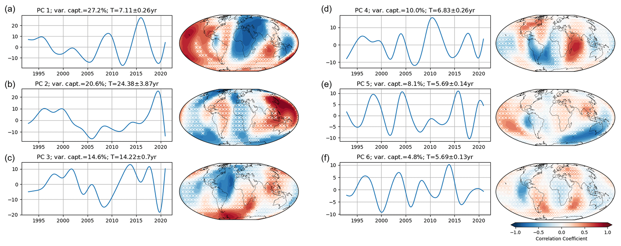
Figure 1 PCs of the magnetic field obtained from PCA (left). The corresponding correlation coefficients between the spatial patterns associated with each PC and the magnetic field are shown on the right. The white cross marks indicate the locations where the correlation significance does not reach the 95 % level.

The second mode captures 20.6 % of the total variance, with a period of T≈24.4 years and the strongest correlations in the northern Pacific Ocean and the Southern Ocean. The third mode (variance captured 14.6 %) shows a decadal oscillation, mostly active in the Atlantic and Southern Ocean, with a small active area close to Indonesia. The fourth PC has an oscillation period of 6.8 years. The signal is mostly active in the western part of the Indian Ocean and around the South American continent. PC5, which accounts for 8.1 %, has a dominant oscillation period of $T=\mathrm{5.7}\pm \mathrm{0.14}$ years, similar to PC6, which accounts for 4.8 % of variance. Both of those modes are separated with a lag of 1.58 years. Even though the dominant period is similar, the two PCs have different spatial patterns and distinguishable eigenvalues according to the rule of thumb of North et al. (1982). PC5 has three lobes of stronger patterns at southern low latitudes and the Bay of Bengal, while the correlated patterns of the PC6 are located around Central America and in the southern part of the Pacific and the Indian Ocean.

Unlike PCA, only three components are found to be significant at the 95 % level in MSSA (Fig. A1b). The pair of ST-EOFs 1 and 2 represents an oscillation of $T=\mathrm{7.1}\pm \mathrm{0.29}$ years, accounting for 37.29 % of the total variance (Fig. 2a). The reconstruction of this mode shows an increase in variability as time advances. We found that the spatial patterns for this mode (Fig. 2c) are identical to the spatial patterns of PC1 from PCA (Fig. 1a), with a spatial correlation of 0.97 between the two patterns.

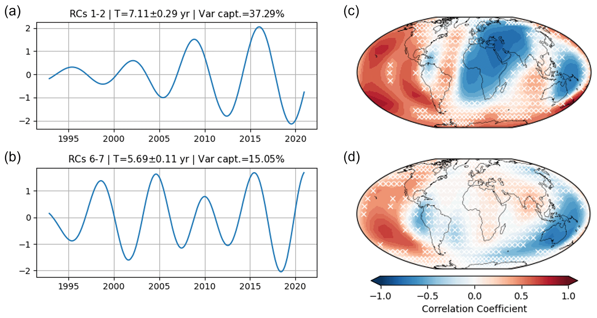
Figure 2 (a) Leading S-PC of RC1–2 that creates an oscillation of 7.1 ± 0.29 years, obtained from MSSA of the magnetic field. (b) Leading S-PC of RC6–7 forming an oscillation of 5.7 ± 0.11 years. As in Fig. 1, panels (c) and (d) show the correlation patterns of the modes of 7.1 and 5.7 years, respectively. The MSSA here uses a window length of M= 110 months. The white cross marks indicate the locations where the correlation significance does not reach the 95 % level.

ST-EOF 6 is also found to be significant at the 95 % level. However, the pair of this component, ST-EOF 7, is only significant at the 90 % level. Together, this pair constructs a mode with a period of 5.7 ± 0.11 years that captures 15.05 % of the total variance (Fig. 2b). The spatial pattern of this mode (Fig. 2d) resembles the spatial pattern of PC5 in PCA (Fig.  1e) but with a stronger correlation in the Pacific area and no lobe in the Bay of Bengal.

In summary, two oscillatory modes appear to be robust in the magnetic field, with periods of T≈7 years and T≈6 years. Besides the temporal properties, the spatial patterns of these modes are also consistent in both techniques.

3.1.2 Gravity field

Similar procedures are applied to the analysis of the gravity field. The significance test in PCA leads us to keep 29 components which together capture up to 99 % of the total variance (Fig. A5).

The first three modes (Fig. 3a–c) do not exhibit the oscillatory behavior observed in the magnetic field modes. The first mode accounts for 40.5 % of the total variance, forming a bi-decadal variability, similar to a polynomial degree 2 of time. The second mode captures 18.7 %. The third mode accounts for 15.4 % of the gravity field variance. Areas with stronger and significant correlations are located mostly in the Southern Hemisphere, extending from the south of the Atlantic Ocean to the western limit of the Pacific Ocean, with weaker correlations on the Asian continent.

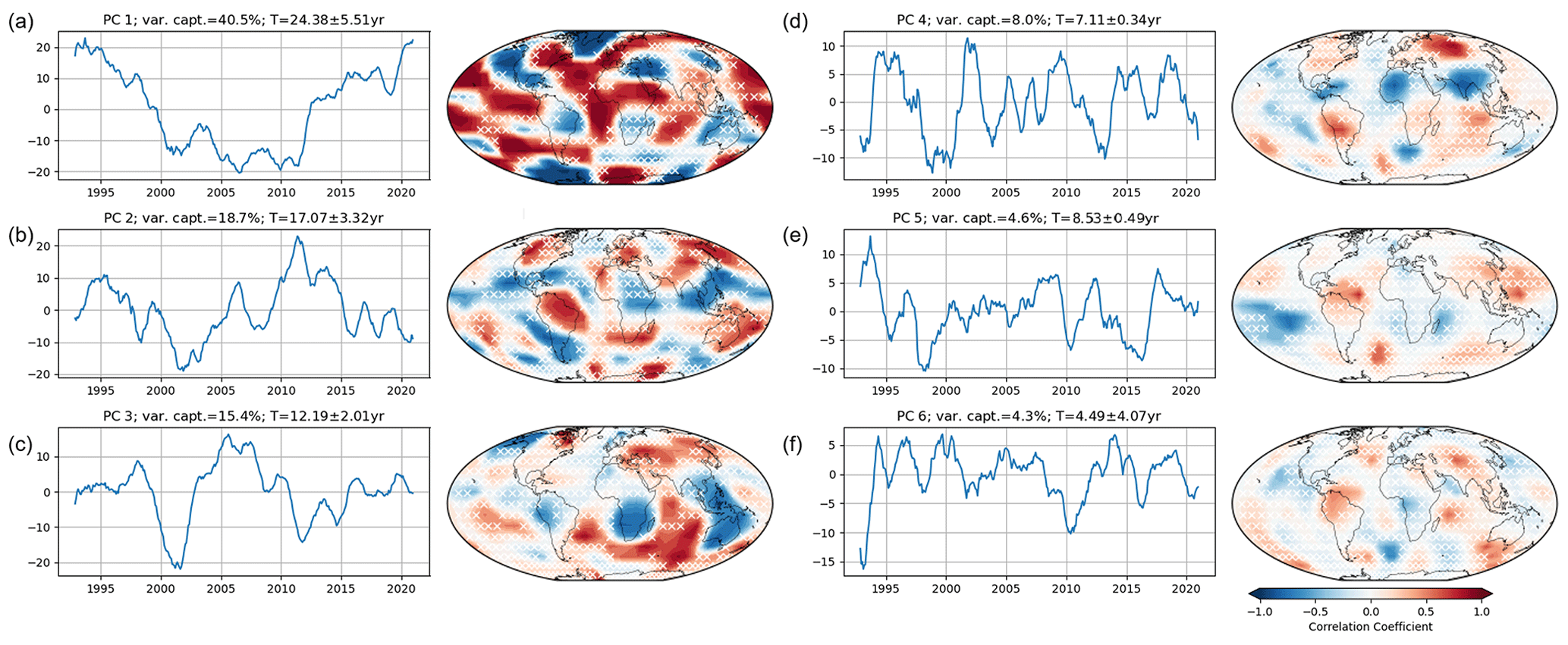
Figure 3 PCs of the gravity field obtained from PCA (a, b, c). The corresponding correlation coefficients between the spatial patterns associated with each PC and the gravity field are shown in panels (d), (e), and (f). The white cross marks indicate the locations where the correlation significance does not reach the 95 % level.

The fourth mode oscillation is dominated by a 7.1-year oscillation and captures 8 % of the total variance. This mode strongly correlates around South and Central America and the northern part of African close to the Gulf of Guinea, and it extends from north to south along the meridian at 100^∘ E. The fifth mode (4.6 %) is dominated by 8.5-year oscillations, with a smaller spatial extent scattered across the oceans. The sixth mode has a variability of T≈4.5 years where the significant correlated areas are scattered all over the globe.

From the Monte Carlo test, we found 17 significant modes at the 95 % level with MSSA (Fig. A5b). Among them, an oscillatory pair of ST-EOFs 5 and 6 constructs a mode with $T=\mathrm{6.8}\pm \mathrm{0.21}$ years (Fig. 4a). Compared to the spatial pattern of PC4 from PCA (Fig. 3d), which has $T=\mathrm{7.1}\pm \mathrm{0.34}$ years, the spatial pattern resulting from MSSA (Fig. 4b) is consistent with its spatial pattern with a spatial correlation of 0.78.

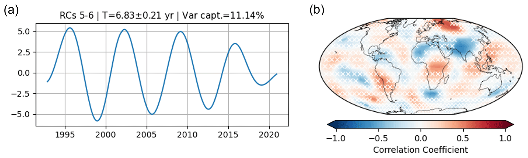
Figure 4 (a) Reconstructed component (RC) of the gravity field with ST-EOFs 5 and 6 obtained from MSSA at a period length of 6.8 ± 0.21 years. (b) Correlation coefficient pattern between the gravity time series and the RCs in (a). The MSSA here uses a window length of M= 110 months. The white cross marks indicate the locations where the correlation significance does not reach the 95 % level.

ST-EOFs 10 and 11 are also significant, showing a mode with a cycle of 3.88 years. The other significant ST-EOFs do not form oscillating pairs and correspond to higher frequencies. As they do not appear in the magnetic field and considering their high frequency, we do not discuss them further in the present study.

The time variability of the 7-year oscillatory modes of the gravity field resembles to some extent those of the magnetic field (r=0.78), although significant differences are visible. The dynamic of higher frequencies is more clearly visible in the gravity field, possibly coming from contamination from faster climate dynamics. While the oscillation amplitude increased with time on the magnetic field, those in the gravity field rather seem to decrease.

The spatial patterns differ between the magnetic and gravity field in the 7-year mode. We will return to the details of the gravity field spatial pattern in Sect. 3.2.

3.2 Joint gravity–magnetic field analysis

We proceed with joint analyses of the magnetic and gravity fields to better highlight the similarities and differences between the two fields. For the joint PCA and MSSA, we concatenate the two normalized potential field data sets into a single multivariate time series. These methods generate common expansion coefficients (PCs) of both fields and two spatial eigenvectors that are presented as correlation maps.

As in the previous section, we first test the significance of the eigenvectors (Fig. B1). The first 43 PCs of the joint PCA are significant against the normal random surrogates (Fig. B1a), which correspond to period lengths between 0.4 and 24.4 years. These significant components together account for 99 % of the total variance.

Figure 5 shows the results from the joint PCA. We find significant oscillatory modes that were identified in the PCA of the individual fields – bi-decadal, decadal, ≈ 7 years, and ≈ 6 years. In the joint analysis, we always find PCs as a trade-off between those with similar periods from the analysis of the individual field (Kutzbach, 1967; Ghil et al., 2002). The associated spatial patterns are analogous to the spatial patterns from the PCA of the separate field with a similar PC period.

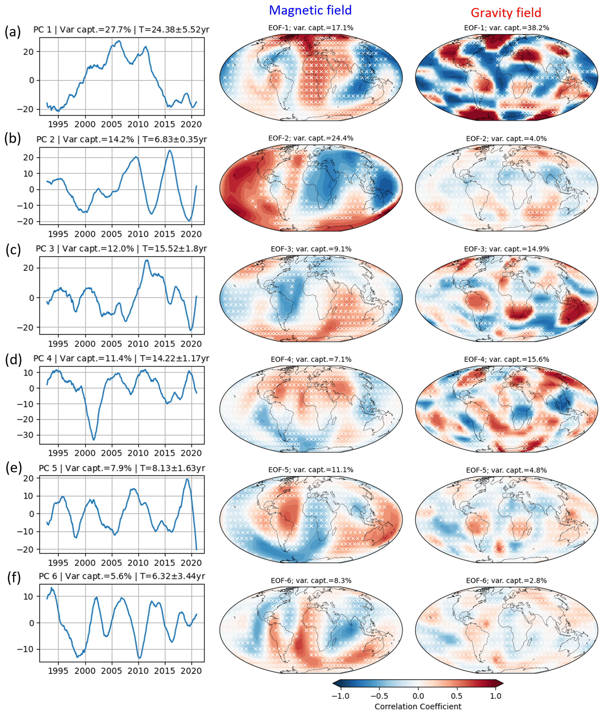
Figure 5 (a–f) PCs obtained from PCA of the joint field. On the right is the correlation map of the magnetic field and gravity field associated with each PC. The percentage of the variance captured by each PC is shown on the top of the time expansion. The portion of the variance captured in each field is mentioned at the top of the correlation map. The white cross marks indicate the locations where the correlation significance does not reach the 95 % level.

The dominant common variability between the two fields corresponds to a long-term behavior, similar to polynomial degree 2 of time (PC1 in Fig. B2a) and to PC1 of the gravity field (Fig. 3a). The spatial patterns are comparable to the ones resulting from the PCA of the individual field above – maps of PC2 for the magnetic field (Fig. 1b) and PC1 for the gravity field (Fig. 3a).

The interannual variation with $T=\mathrm{6.83}\pm \mathrm{0.35}$ years is captured by PC2, with 14.2 % of the total variance captured. The PC of this mode resembles a trade-off of the separate PC in the individual fields of the associated period, i.e., dominant oscillations of 7 years found in PC1 of the magnetic field with higher-frequency dynamics from the gravity field. The spatial patterns of this mode are akin to the ones of PC1 in the magnetic field (Fig. 1a) and PC4 in the gravity field (Fig. 3d), except for the areas in South America and the Indian Ocean.

The third mode exhibits a time variability of 15.52 ± 1.8 years. The resulting spatial patterns are consistent with the third mode from the separated analysis for the magnetic field (Fig. 1c) and the second mode for the gravity field (Fig. 3b). The fourth PC captures the third modes of the gravity-field-separated PCA (Fig. 3c) and of the magnetic field (Fig. 1c) with a cycle of 14.22 ± 1.17 years, but both exhibit significantly different patterns with respect to that from the separated analysis.

From the joint MSSA, seven ST-EOFs are identified as significant from the Monte Carlo test (Fig. B1b). ST-EOFs 3 and 5 are in phase quadrature and form an oscillatory pair of 7.42 ± 0.33 years (Fig. 6a), which accounts for 21.8 % of the variance captured. This mode period is consistent with that from the mode found in the abovementioned MSSAs of the separated individual field. The mode amplitude increases with time but is significantly less than in the separated MSSA of the magnetic field (Fig. 2a). The spatial patterns are similar to those from the separated fields.

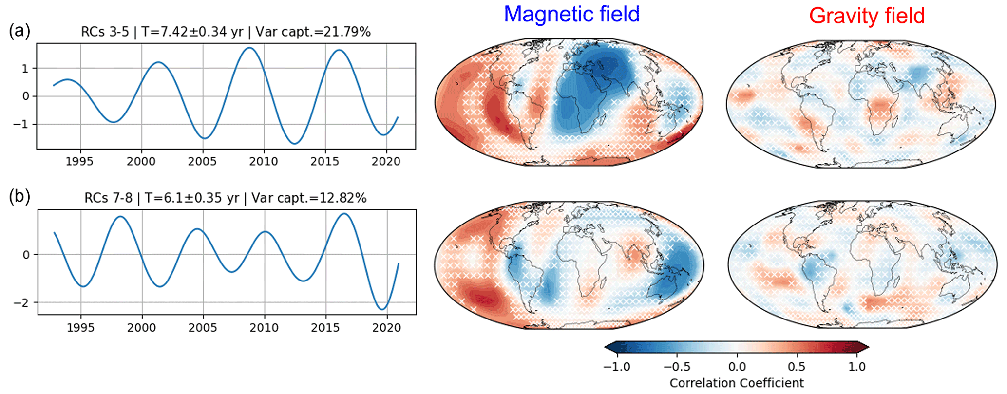
Figure 6 Reconstruction of the joint field of oscillatory pairs at a period length of 7.42 ± 0.33 years (a) and 6.1 ± 0.35 years (b). The correlation patterns of the magnetic and gravity field of each mode are given on the right side. The MSSA here uses a window length of M= 110 months. The white cross indicates the areas with insignificant correlations at the 95 % level.

An oscillatory pair with a period length of 6.1 ± 0.35 years is also found to be significant, formed by the pair of ST-EOFs 7 and 8 (Fig. 6b). This mode is consistent with the 6-year mode found in the magnetic field, where this period is not found in the MSSA of the gravity field.

Figure 7 shows the PCs associated with gravity and magnetic fields separately, obtained from the joint SVD analysis. The first 14 PCs are tested to be significant (Fig. B1c). Consistent with the PCA of the separate fields and the respective time variability of the gravity and magnetic fields, the temporal variations in the gravity field also contain a noticeably higher frequency than the magnetic field.

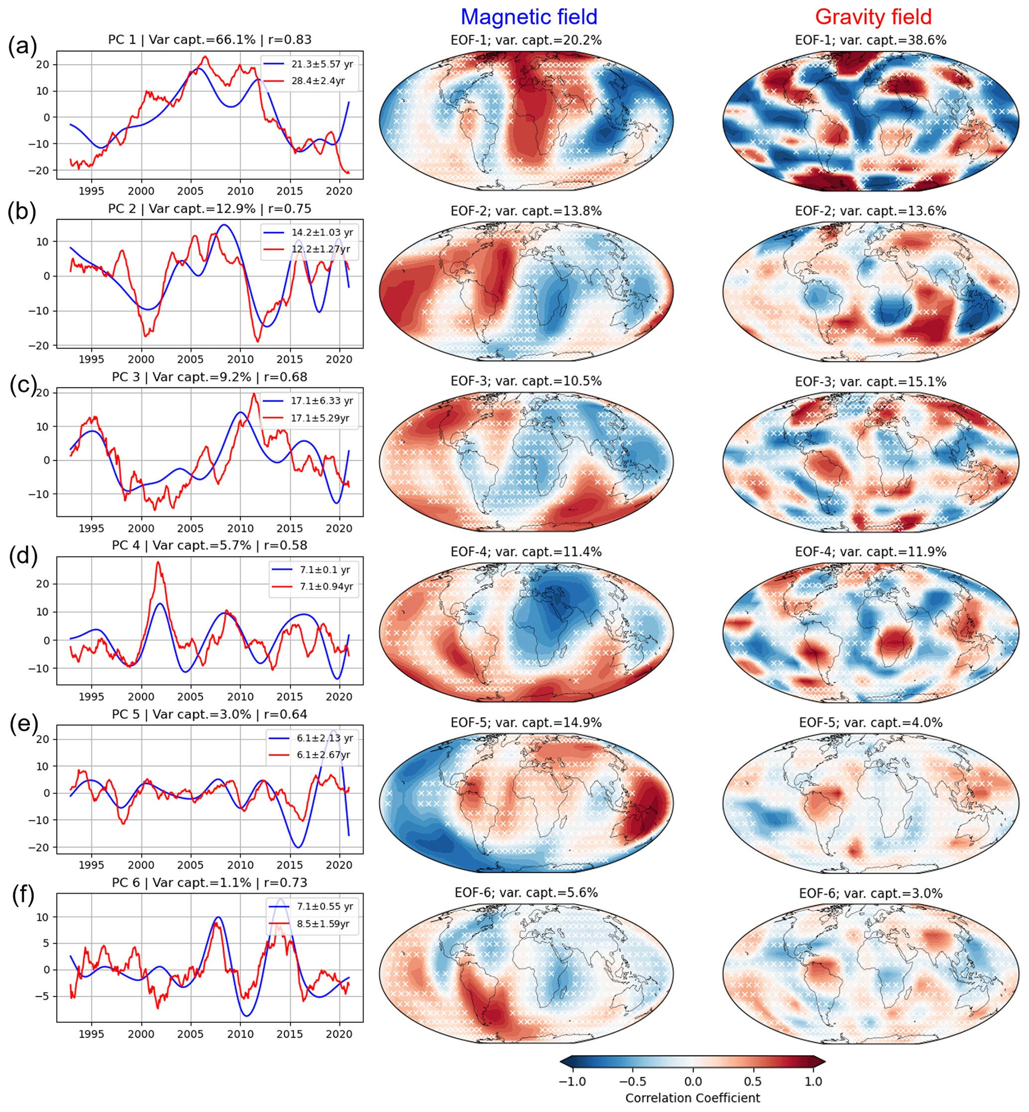
Figure 7 (a–f) The first six PCs of the magnetic (blue line) and gravity field (red line) obtained from the joint SVD technique. The corresponding dominant period and the Pearson's correlation coefficient (r) are written in the legend. The correlation patterns of the magnetic and gravity field of each mode are given on the right side. The white cross indicates the areas with insignificant correlations at the 95 % level.

Bi-decadal and decadal variabilities dominate the first three modes in the SVD analysis, with similar spatial patterns compared to the results of the PCA of the joint field. However, the time series length of 28 years that we use in this study limits the reliability of detecting such long-term variation, and thus further elaboration on this behavior is beyond the scope of this paper.

For the fourth mode, we find an oscillatory period of 7.1 years, with a temporal correlation coefficient r=0.58. The spatial patterns of the magnetic field in this mode resemble the 7-year modes from other analyses. In contrast, the associated gravity field mode mixes that of periods 12.2 and 7 years from the separated analysis (Fig. 3c–d). The spatial patterns from this analysis are notably different from those from other analyses.

The fifth PC exhibits a dominant oscillation of T≈ 6.1 years, which captures 3 % of the total variance. The spatial patterns found in this mode are comparable to the ones resulting from the joint MSSA (Fig. 6b), where the significant zones are consistent across these two different results.

The results in the joint field analyses are consistent with the ones in the separate analysis of the magnetic and gravity fields (Sect. 3.1). During the 7-year period, the spatial patterns of the magnetic field from all analyses consistently displayed similar general geographic patterns, as do the gravity field maps. Nonetheless, the difference between the magnetic and gravity fields was noticeable, as shown in the analyses of each field.

Meanwhile, the oscillation at a 6-year period is detected in all analyses except in the MSSA of the gravity field. Despite the use of various types of analysis and input combinations, the space and time signatures of these modes exhibited sufficient similarities to support the validity of their detection. This suggests that the results are robust and reliable.

4 Discussion and conclusions

We used the co-analysis of magnetic and gravity fields to separate between climate-induced and internal – probably core – signatures in the gravity field data. The application of different techniques also allows us to mine for common behavior between magnetic and gravity fields and to assess the robustness of the associated principal components of the time series. The consistency of those common behaviors over different data sets (see also the Appendix) further demonstrates the robustness of those signatures and confirms the obtained time series and space patterns.

The applied analyses provide rich information about the temporal and spatial behavior of the magnetic and gravity fields. In the following, we summarize these results in two dedicated figures.

A summary of significant mode periods is displayed in Fig. 8. As expected, more modes with short-term variability (of the order of a couple of years) are found in the gravity-only-based analysis. The dynamics of the mass redistribution on the Earth's surface are represented in the modes with higher frequencies (Gruber et al., 2011), which are mainly related to the climate system time variability. With a maximum series length of 28 years, we focus here on oscillations with periods longer than 4 years and shorter than 14 years.

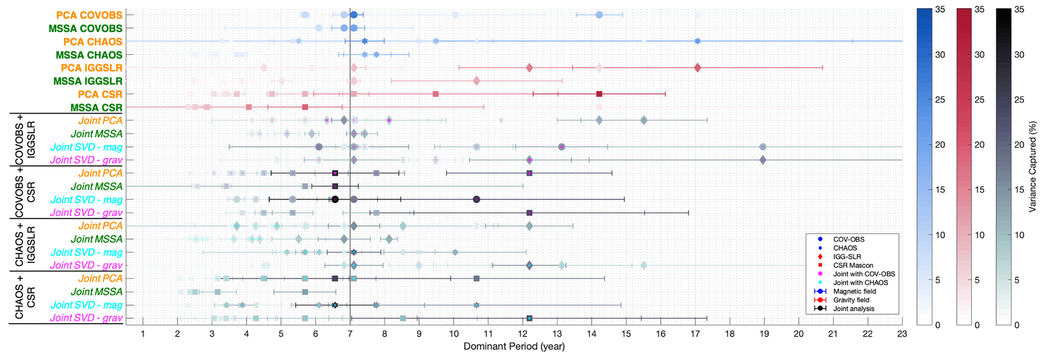
Figure 8 Significant mode periods from each analysis, along with the uncertainty of the estimated dominant period. The error bars show the corresponding period length error estimate (1σ). The methods and data sets are listed in the y axis: PCA (orange), MSSA (green), and joint SVD (magenta and cyan). Individual field analyses are indicated in bold text, and joint field analyses are in italics. Each data set is displayed with different symbols. The blue, red, and black represent the results of magnetic, gravity, and joint fields, respectively. The color bars show the percentage of the variance captured by each mode.

Modes within a period range of 6.5–7.5 years are found to be significant in 20 analyses out of 24. In the following, this is called the “7-year mode” and it captures on average 13.8 % of the variance, with a maximum of 35.1 % in the PCA of the COV-OBS.x2. The amplitude evolution of the PCs detected in the separated analysis and in the SVD exhibits differences: an increase for the magnetic field (Figs. 1, 2) and a slight decrease for the gravity field (Fig. 3, 4, 7).

Unlike MSSA, SVD and PCA do not favor pseudo-periodic behavior. Finding time oscillations in SVD and PCA results is thus a piece of evidence that this periodic behavior is significant in both time series.

Besides the 7-year mode, oscillations with a period T≈ 6 years are also found to be significant, appearing in 16 analyses out of 24. Taking into account the uncertainty of the period estimates and also the frequency resolution of the spectrum (Lathi and Green, 2005, e.g.,), it is not possible to exclude the possibility that the modes at periods 6 and 7 years correspond to the same physical phenomena. However, considering that the 6-year oscillation mostly occurs simultaneously with the 7-year one and that their spatial patterns are different (Fig. C1), they are more probably the signatures of distinct phenomena.

The areas defined in Fig. 9 as significant for the magnetic field are close to those indicated in different studies and related to a 7-year oscillation (e.g., Buffett and Matsui, 2019; Aubert and Gillet, 2021; Gillet et al., 2022a, b). Our results coincide with those of previous studies and confirm our approach. Consequently, we elaborate no more on the magnetic aspect in the present paper.

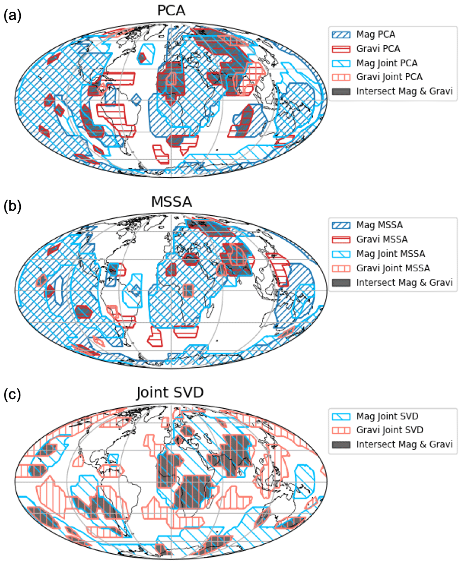
Figure 9 Maps of the areas associated with the 7-year mode where the correlation coefficients between the magnetic field (blue) or the gravity field (red) and the obtained time PC from PCA (a), MSSA (b), and joint SVD (c) are significant at the 95 % level. The areas where both the magnetic and gravity fields are significantly correlated with the 7-year mode are marked in grey.

Figure 9 shows locations for the 7-year mode of the magnetic and gravity fields and underlines those where both are significant, without, however, a clear correlation between those two space patterns. This is not surprising, considering that the transformation of core processes into mass and into magnetic anomalies are different and probably rely on different properties of the core and of the CMB. In addition, the 7-year mode in the gravity field might still be influenced by residual signals from surface processes, leading to differences in spatial behavior reflected in the gravity field and complicating our interpretation of the observed gravity field being solely driven by the Earth's core processes.

We note that there are still limitations in isolating the signal linked to the core dynamics that hinder us from providing a deeper or more complete analysis. Dumberry and Mandea (2022) pointed out that interpreting the amplitude and spatial pattern of the gravity signal due to core processes is prone to ambiguity since the resulting signal is relatively weak compared to that from mass anomalies in the crust and mantle. However, detecting core signatures in the gravity field can be facilitated through temporal variations, with a careful analysis of all sources presented in the gravity field. Although the spatial patterns between the two fields show some discrepancies, we consider the temporal changes in the gravity field to align with the signature of the core contribution which is observed in the geomagnetic field.

Some possible mechanisms of the dynamic core processes that can perturb the gravity field have been previously proposed: changes in the density field within the volume of the core (Dumberry, 2010), the dissolution–crystallization process at the CMB (Mandea et al., 2015), pressure anomalies at the CMB that entrain the elastic deformation in the Earth (see Greff-Lefftz et al., 2004; Dumberry and Bloxham, 2004; Dumberry, 2010), and the reorientation of the inner core along with its lateral heterogeneity (Gillet et al., 2021; Dumberry and Mandea, 2022). However, the quantification of the gravitational perturbation due to those proposed mechanisms remains challenging, particularly in elucidating the perturbations at such a scale as that of the gravity field patterns. Further investigation is necessary, for example, to estimate the gravitational effect of the core dynamics, particularly on the interannual timescale and at higher harmonic degrees. Building complete models of such motions is beyond the scope of this paper.

The results presented here are encouraging in terms of looking for information on the dynamics of the Earth's core in other data sets, such as the gravity field, which might provide ancillary input as a base to build models that enhance our understanding of the properties and dynamics of the core. Over the upcoming years, longer magnetic and gravity observations will be available, allowing for a better separation between climate- and core-induced signatures. More refined work on separating the sources of the observed magnetic and gravity fields while taking into account the physical properties might also help to better isolate and understand different components in the Earth's core system.

Appendix A: Analysis of individual fields

A1 Magnetic fields

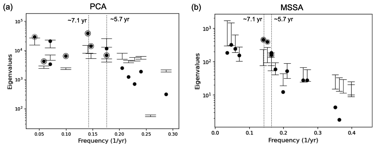
Figure A1 Significant test of PCs using a Monte Carlo-type hypothesis. (a) Comparison of eigenvalues in PCA between COV-OBS.x2 and surrogates based on AR(p). (b) Spectral properties of COV-OBS.x2 obtained from MSSA, with a subsequent varimax rotation using ST-EOFs 1–13. The estimated eigenvalues are plotted in black dots as a function of their corresponding frequency. The lower and upper ticks on the error bars indicate 5 % and 95 % from a Monte Carlo test with scaled procrustes target rotation of T-EOFs (Groth and Ghil, 2015). The significant PCs are circled.

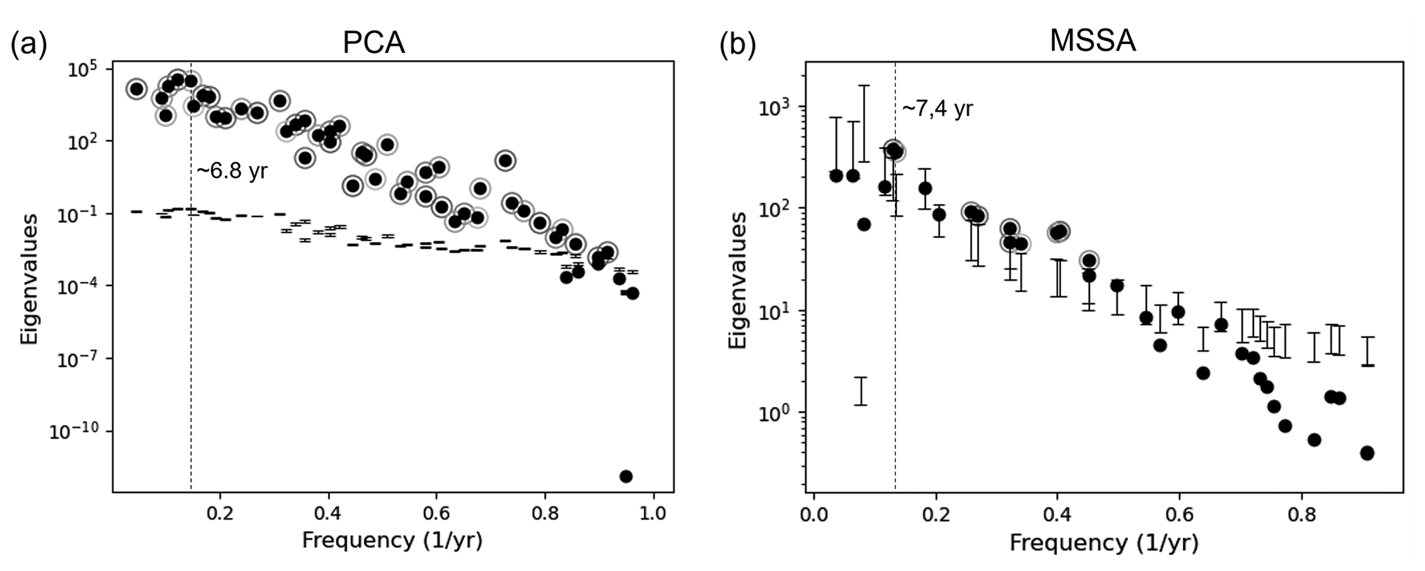
Figure A2 Significant test of PCs using a Monte Carlo-type hypothesis. (a) Comparison of eigenvalues in PCA between CHAOS-7.12 and surrogates based on AR(p). (b) Spectral properties of CHAOS-7.12 obtained from MSSA, with a subsequent varimax rotation using ST-EOFs 1–21. The estimated eigenvalues are plotted in black dots as a function of their corresponding frequency. The lower and upper ticks on the error bars indicate 5 % and 95 % from a Monte Carlo test with scaled procrustes target rotation of T-EOFs (Groth and Ghil, 2015). The significant PCs are indicated in circle.

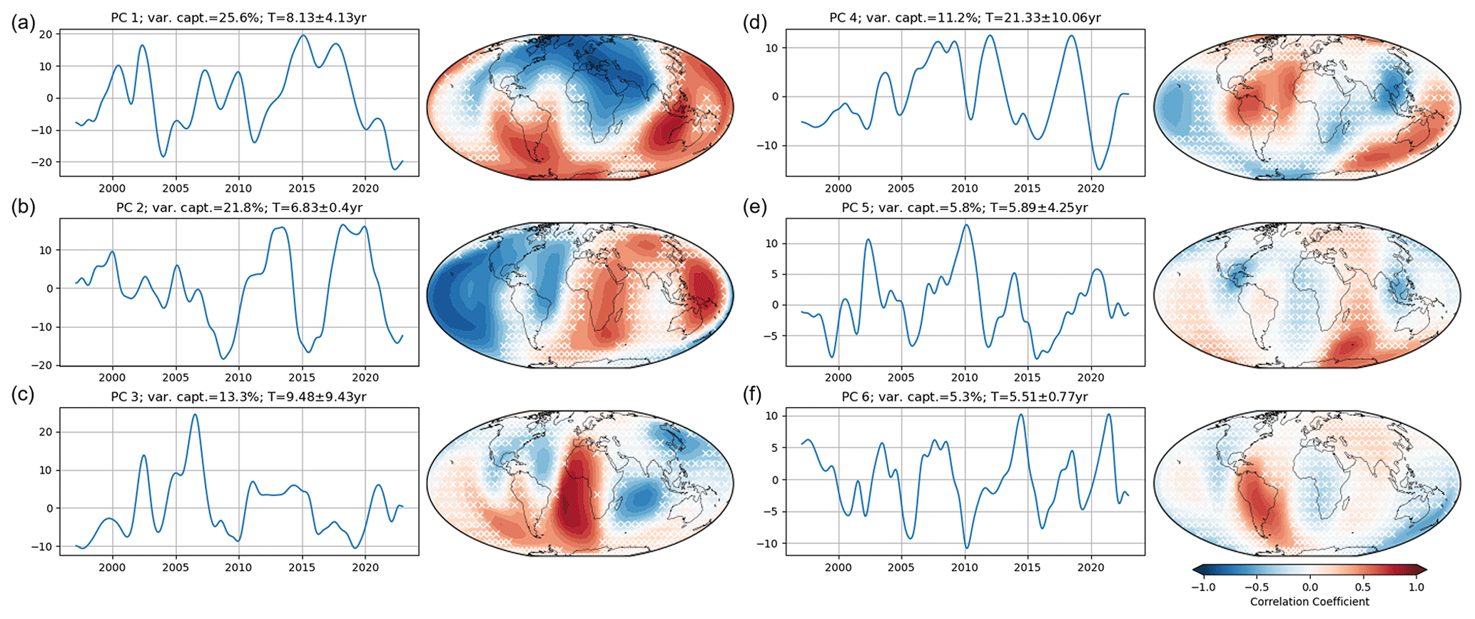
Figure A3 PCs and their corresponding spatial correlation pattern of CHAOS-7.12 obtained from PCA.

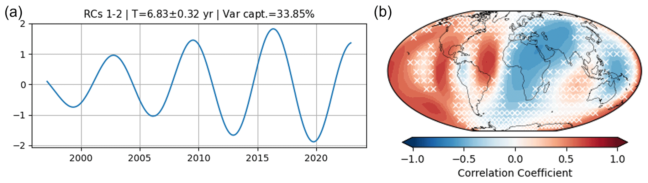
Figure A4 (a) Leading S-PC of RC1–2 that creates an oscillation of 6.8 years, obtained from MSSA of CHAOS-7.12. As in Fig. 1, panel (b) shows the correlation patterns of the mode of 6.8 years. The white cross indicates insignificant correlation at the 95 % level.

A2 Gravity fields

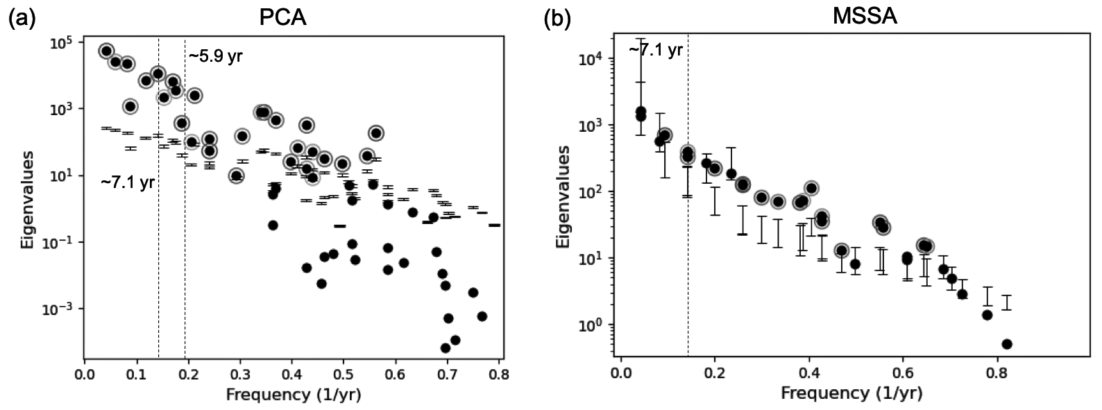
Figure A5 Significant test of PCs using a Monte Carlo-type hypothesis. (a) Comparison of eigenvalues in PCA between IGG-SLR and surrogates based on AR(p). (b) Spectral properties of IGG-SLR obtained from MSSA, with a subsequent varimax rotation. The estimated eigenvalues are plotted in black dots as a function of their corresponding frequency. The lower and upper ticks on the error bars indicate 5 % and 95 % from a Monte Carlo test with scaled procrustes target rotation of T-EOFs (Groth and Ghil, 2015). The significant PCs are circled.

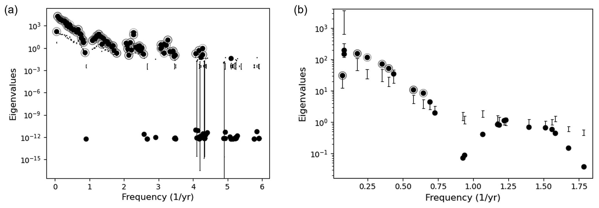
Figure A6 Significant test of PCs using a Monte Carlo-type hypothesis. (a) Comparison of eigenvalues in PCA between GRACE CSR mascon and surrogates based on AR(p). (b) Spectral properties of GRACE CSR mascon obtained from MSSA, with a subsequent varimax rotation. The estimated eigenvalues are plotted in black dots as a function of their corresponding frequency. The lower and upper ticks on the error bars indicate 5 % and 95 % from a Monte Carlo test with scaled procrustes target rotation of T-EOFs. The significant PCs are circled.

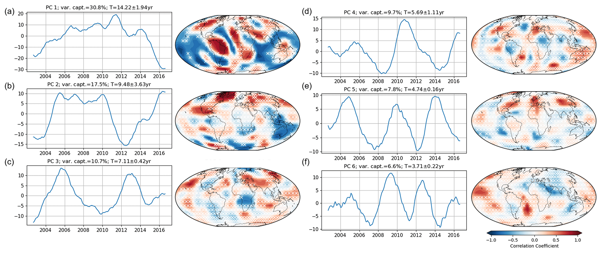
Figure A7 PCs and their corresponding spatial correlation pattern of GRACE CSR mascon obtained from PCA.

Appendix B: Joint analysis

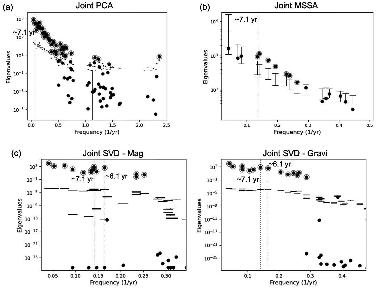
Figure B1 Significant test of PCs using a Monte Carlo-type hypothesis. (a) Comparison of eigenvalues from coupled PCA of the joint fields and surrogates based on AR(p). (b) Spectral properties of joint fields obtained from MSSA, with a subsequent varimax rotation. (c) Comparison of eigenvalues in SVD analysis between joint fields (COV-OBS.x2 and IGSS-SLR) and surrogates based on AR(p). The estimated eigenvalues are plotted in black dots as a function of their corresponding frequency. The lower and upper ticks on the error bars indicate 5 % and 95 % from a Monte Carlo test with scaled procrustes target rotation of T-EOFs (Groth and Ghil, 2015). The significant PCs are circled.

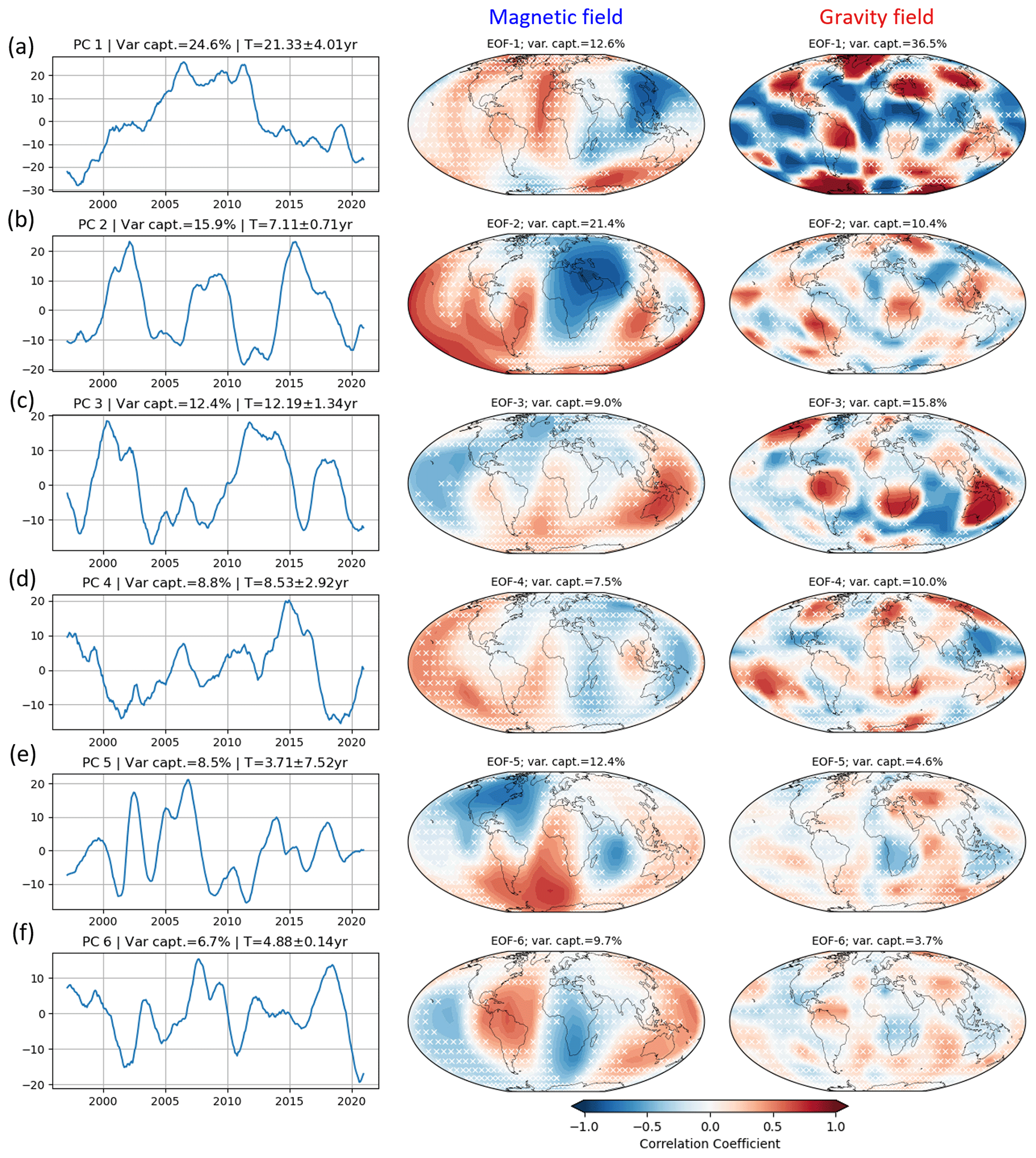
Figure B2 (a–f) PCs obtained from PCA of the joint field. On the right is the correlation map of the CHAOS-7.12 and IGG-SLR associated with each PC. The percentage of the variance captured by each PC is shown on the top of the time expansion. The portion of the variance captured in each field is mentioned at the top of the correlation map. The white cross indicates the areas with insignificant correlations at the 95 % level.

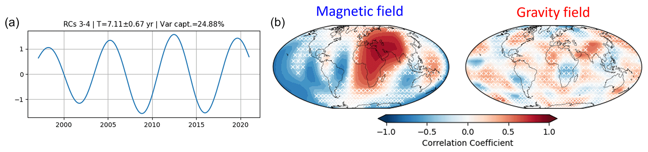
Figure B3 Reconstruction of the joint field of oscillatory pairs at a period length of 7.1 years. The correlation patterns of CHAOS-7.12 and IGG-SLR are given on the right side. The MSSA here uses a window length of M= 110 months. The white cross indicates the areas with insignificant correlations at the 95 % level.

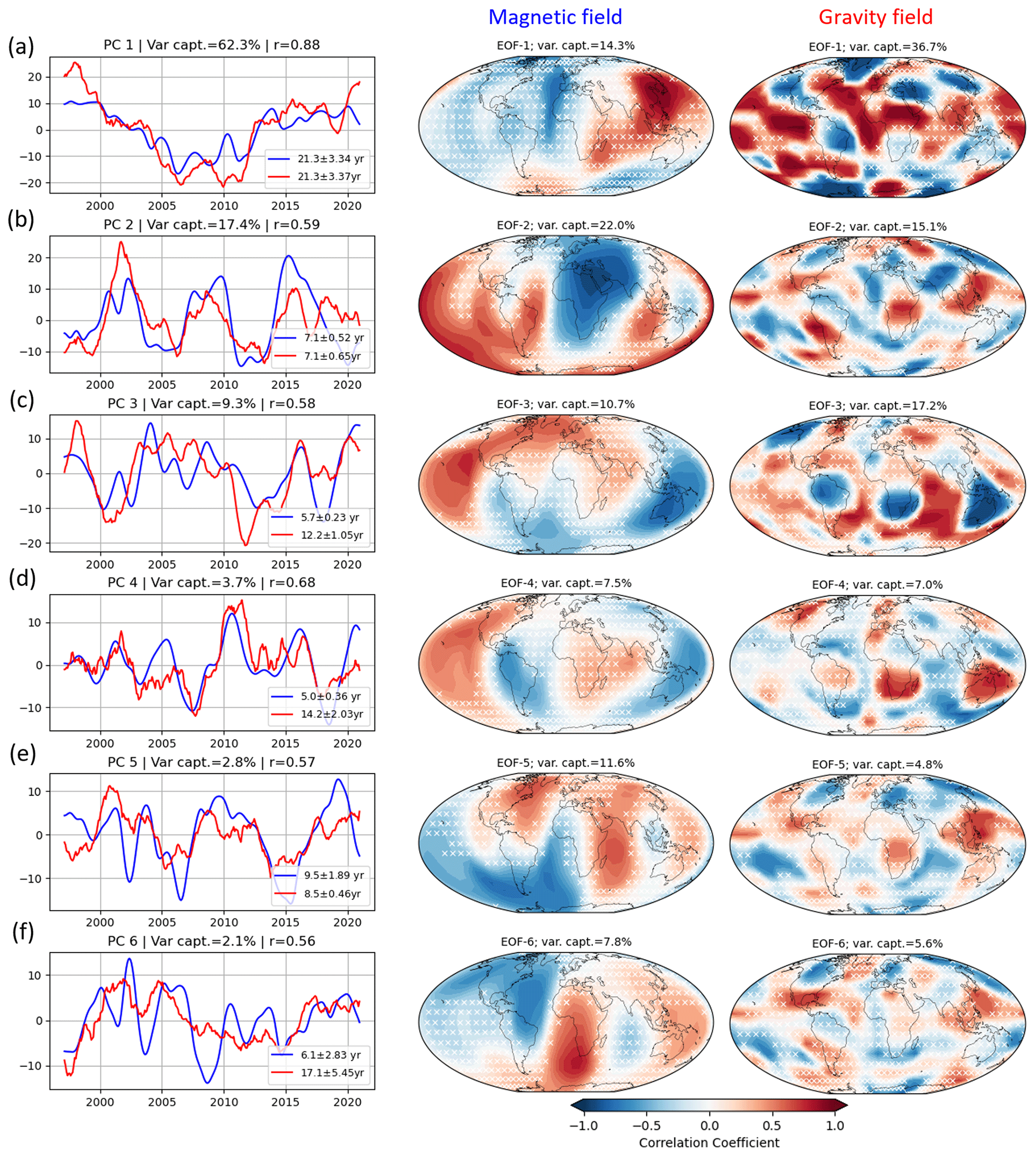
Figure B4 (a–f) The first six PCs of the magnetic (blue line) and gravity field (red line) obtained from the joint SVD technique of CHAOS-7.12 and IGG-SLR. The corresponding dominant period is written in the legend. The correlation patterns of the magnetic and gravity field of each mode are given on the right side. The white cross indicates the areas with insignificant correlations at the 95 % level.

Appendix C: Common spatial properties of 6-year mode

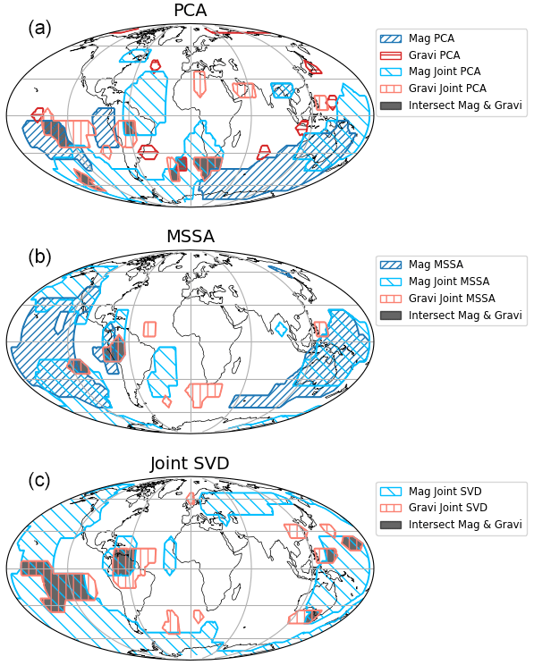
Figure C1 Scatter of areas associated with the 6-year mode where the correlation coefficients between the potential fields and the obtained time PC from PCA (a), MSSA (b), and joint SVD (c) are significant. The layout is the same as for Fig. 9.