the Creative Commons Attribution 4.0 License.
the Creative Commons Attribution 4.0 License.
 | 18 Jan 2023
Utilisation of probabilistic magnetotelluric modelling to constrain magnetic data inversion: proof-of-concept and field application
Hoël Seillé
Mark D. Lindsay
Gerhard Visser
Vitaliy Ogarko
Mark W. Jessell
We propose, test and apply a methodology integrating 1D magnetotelluric (MT) and magnetic data inversion, with a focus on the characterisation of the cover–basement interface. It consists of a cooperative inversion workflow relying on standalone inversion codes. Probabilistic information about the presence of rock units is derived from MT and passed on to magnetic inversion through constraints combining structural constraints with petrophysical prior information. First, we perform the 1D probabilistic inversion of MT data for all sites and recover the respective probabilities of observing the cover–basement interface, which we interpolate to the rest of the study area. We then calculate the probabilities of observing the different rock units and partition the model into domains defined by combinations of rock units with non-zero probabilities. Third, we combine these domains with petrophysical information to apply spatially varying, disjoint interval bound constraints (DIBC) to least-squares magnetic data inversion using the alternating direction method of multipliers (or ADMM). We demonstrate the proof-of-concept using a realistic synthetic model reproducing features from the Mansfield area (Victoria, Australia) using a series of uncertainty indicators. We then apply the workflow to field data from the prospective mining region of Cloncurry (Queensland, Australia). Results indicate that our integration methodology efficiently leverages the complementarity between separate MT and magnetic data modelling approaches and can improve our capability to image the cover–basement interface. In the field application case, our findings also suggest that the proposed workflow may be useful to refine existing geological interpretations and to infer lateral variations within the basement.
- Article
(6331 KB) - Full-text XML
- BibTeX
- EndNote


Geophysical integration has been gaining traction in recent years, be it when two or more datasets are inverted simultaneously (i.e. joint inversion) or when the inversion of a geophysical dataset is used to constrain another (i.e. cooperative inversion). A number of approaches for joint modelling have been developed with the goal of exploiting the complementarities between different datasets (see, for instance, the reviews of Lelièvre and Farquharson, 2016, and Moorkamp et al., 2016, and references therein). As summarised in the review of Ren and Kalscheuer (2019), “joint inversion of multiple geophysical datasets can significantly reduce uncertainty and improve resolution of the resulting models”. This statement remains valid, be it for the modelling of a single property (e.g. resistivity for joint controlled-source electromagnetic and magnetotelluric (MT) data or density for joint gravity anomaly and gradiometric data) or of multiple properties (e.g. the joint inversion of seismic and gravity data to model P-wave velocity and density). In the second case, joint inversion approaches can be grouped into two main categories based on the hypothesis they rely on. Structural approaches allow for the joint inversion of datasets with differing sensitivities to the properties of the subsurface through the premise that geology requires spatial variations in inverted properties to be co-located. Structural constraints can then be used as a way to link two or more datasets jointly inverted for by encouraging structural similarity between the inverted models (Haber and Oldenburg, 1997; Gallardo and Meju, 2003). Alternatively, petrophysical approaches utilise prior petrophysical information (e.g. from outcrops, boreholes, or the literature) to enforce certain statistics in the recovered model so that it resembles the petrophysical measurements' (Lelièvre et al., 2012; Sun and Li, 2015; Giraud et al., 2017; Astic and Oldenburg, 2019). Whereas structural and petrophysical approaches are well suited to exploit complementarities between datasets in a quantitative manner, running joint inversion might be, in practice, challenging due to, for instance, the risk of increased non-linearity of the inverse problem (see, e.g. the L surface using the cross-gradient constraints in Martin et al., 2021, and approaches adapting coupling during inversion, e.g. Heincke et al., 2017), the necessity to balance the contribution of the different datasets inverted (Bijani et al., 2017) and resolution mismatches (Agostinetti and Bodi, 2018).
In this contribution, we present a new multidisciplinary modelling workflow that relies on sequential, cooperative modelling. It follows the same objectives as the two categories of joint inversion mentioned above in that structural information is passed from one domain to the other and uses petrophysical information to link domains. The development of the sequential inversion scheme we present is motivated by a similar idea as Lines et al. (1988), who states that “the inversion for a particular data set provides the input or initial model estimate for the inversion of a second data set”. A further motivation is to design a workflow capable of integrating the inversion of two or more datasets quantitatively using standalone modelling engines that run independently.
In this paper, the workflow is applied to the sequential inversion of MT followed by magnetic data, taking into account the importance of robustly constraining the thickness of the regolith in hard-rock imaging and mineral exploration. This is motivated by the relative paucity of works considering cooperative workflows to integrate MT and magnetic data together with the recent surge in interest for the characterisation of the depth to basement interface in mineral exploration, despite these two geophysical methods being part of the geoscientists' toolkit for depth to basement imaging. Historically, MT has often been integrated with other electromagnetic methods or with seismic data (e.g. Gustafson et al., 2019; Peng et al., 2019), and with gravity to a lower extent (see review of the topic of Moorkamp, 2017). It is, however, seldom modelled jointly with magnetic data unless a third dataset is considered (e.g. Oliver-Ocaño et al., 2019; Zhang et al., 2020; Gallardo et al., 2012; Le Pape et al., 2017). We surmise that this is because (i) the interest for integrating MT with other disciplines arose primarily in oil and gas and geothermal studies and relied on structural similarity constraints for reservoir or (sub)salt imaging, (ii) the difference in terms of spatial coverage between the two methods elsewhere, (iii) the differences in terms of sensitivity to exploration targets and (iv) the difficulty to robustly correlate electrical conductivity and magnetic susceptibility. Bearing these considerations in mind, we developed a workflow incorporating MT and magnetic inversion with petrophysical information and geological prior knowledge.
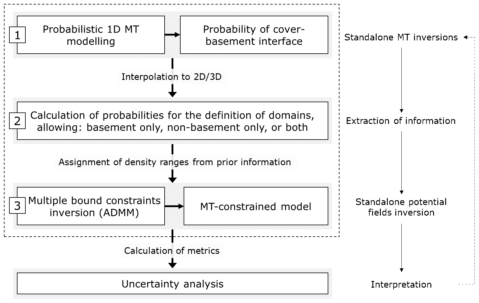
Figure 1MT–magnetic integration workflow summary showing the role of the different techniques.
In the workflow we develop, we exploit the differences in sensitivity between MT and magnetic data. On the one hand, the MT method, used in a 1D probabilistic workflow as presented here, is well suited to recover vertical resistivity variations and interfaces, especially in a sedimentary basin environment (Seillé and Visser, 2020). MT data are, however, poorly sensitive to resistors, particularly when they are overlaid by conductors (e.g. Chave et al., 2012), which makes it difficult to differentiate between highly resistive features, such as intra-basement resistive intrusions. On the other hand, magnetic data inversion is more sensitive to lateral magnetic susceptibility changes and to the presence of vertical or tilted structures or anomalies. Bearing this in mind, we first derive structural information across the studied area in the form of probability distributions of the interfaces between geological units, extracted from the interpolation of probabilistic 1D MT data inversion. From there, the probability of occurrence of geological units can be estimated in 2D or 3D. These probabilities are used to divide the area into domains where only specific units can be observed (e.g. basement, sedimentary cover, or both). Such domains are then passed to magnetic data inversion, where they are combined with prior petrophysical information to derive spatially varying, disjoint interval bound constraints that can consider multiple intervals in every model cell. Such constraints are enforced using the alternating direction method of multipliers for 2D or 3D inversion (ADMM; see Ogarko et al., 2021a, for application to gravity data using geological prior information and Giraud et al., 2021c, for MT-constrained gravity inversion). Finally, uncertainty analysis of the recovered magnetic susceptibility model is performed, and rock unit differentiation allows for controlling the compatibility of magnetic inversion results with the MT data. The workflow is summarised in Fig. 1, as applied to 1D MT inversions. In this paper, we apply this workflow to 2D magnetic data inversion, but it is applicable in 3D.
The remainder of this paper is organised as follows. We first introduce the methodology and summarise the MT and magnetic standalone modelling procedures we rely on. We then introduce the proof of concept in detail using a realistic synthetic case study based on a geological model of the Mansfield area (Victoria, Australia), which we use to explore the different possibilities for integrating MT-derived information and petrophysics offered by our workflow. Following this, we present a field application using data from Cloncurry (Queensland, Australia) where we tune our approach to the specificity of the area. Finally, this work is placed in the broader context of geoscientific modelling, and perspectives for future work are exposed in the discussion section.
2.1 MT inversion for interface probability
The MT method is a natural source electromagnetic method. Simultaneous measurements of the fluctuations of the magnetic and electric fields are recorded at the Earth's surface under the assumption of a plane wave source. The relationship between the input magnetic field H and the induced electrical field E, which depends on the distribution of the electrical conductivities in the subsurface, is described by the impedance tensor Z, as follows:
Resistivity models derived from MT data are found by forward modelling and inversion of the impedance tensor Z, generally using gradient-based deterministic methods (see, e.g. Rodi et al., 2012). Deterministic approaches provide a single solution that minimises the objective function considered during the inversion, but limited information of the uncertainty around this model can be derived. A global characterisation of the uncertainty is possible using a Bayesian inversion framework, but its expensive computing cost limits its application to approximated and/or fast forward modelling solvers (Conway et al., 2018; Manassero et al., 2020; Scalzo et al., 2019). In this study, we alleviate this by considering a local 1D behaviour of the Earth. While this assumption can stand within layered sedimentary basins, it may fail in more complex geological environments. As we describe below, we account for this source of uncertainty in our Bayesian inversions.
Within the context of Bayesian inversion, the solution of the inverse problem consists of a posterior probability distribution, calculated from an ensemble of models fitting the data within uncertainty. The posterior probability distribution p(mMT|dMT) is obtained using Bayes' theorem, defined as
The prior distribution p(mMT) contains prior information on the model parameters mMT. In this work, we assume a relatively uninformed prior knowledge, using a uniform prior distribution on the logarithm of the electrical resistivity bounds with values set between −2 and 6 log10 Ω m. Using a uniform prior with such wide boundaries allows the inversion to be mainly data driven and to remain independent from assumptions about the distribution of electrical resistivity into the Earth. A Gaussian likelihood function p(dMT|mMT) defining the data fit is used
The term inside the exponential is the data misfit, which is the distance between observed data dMT and simulated data gMT(mMT), scaled by the data covariance matrix Cd, which defines data errors and their correlation across frequencies. We consider two main sources of uncertainty to calculate Cd:
-
data processing errors, which we model introducing a matrix Cp;
-
errors introduced by the violation of the 1D assumption when using 1D models, which we model introducing Cdim.
Both sources of uncertainty are included in the calculation of Cd, defined as . In our calculation, we first define Cp, the covariance matrix accounting for the EM noise and measurement errors, which are estimated during MT data processing. In this study we assume uncorrelated processing noise across frequencies, reducing Cp to a diagonal matrix.
Following this, we define Cdim as the dimensionality covariance matrix accounting for the discrepancy between 1D models and the multi-dimensional Earth that the data is sensitive to. To characterise and quantify this discrepancy and to translate it into a dimensionality error for use within 1D probabilistic inversion, we use the workflow developed by Seillé and Visser (2020). We first analyse the characteristics of the MT phase tensor for all sites at all frequencies. The MT phase tensor is derived from the impedance tensor Z. Characterising the phase tensor symmetry using its invariants (skewness β and ellipticity λ), the presence of 2D and 3D structures affecting the MT data as a function of frequency can be inferred (Caldwell et al., 2004). To quantify how much error non-1D structures introduce in 1D modelling, Seillé and Visser (2020) developed a dimensionality error model. This model is derived using a supervised machine learning approach (regression tree), trained on a large collection of synthetic responses containing many 2D and 3D effects. As a result, it maps the phase tensor parameters derived from the observed data into dimensionality uncertainties to compensate for the limitations of the 1D assumption when performing 1D inversion, with larger errors assigned to data presenting important 2D or 3D effects. This dimensionality uncertainty Cdim is then added to the existing data processing uncertainty Cp, such that the inversion considers both sources of uncertainty in Cd. This approach prevents 1D inversion from fitting 2D or 3D responses. When it is used in a probabilistic inversion scheme, it permits a correct estimation of model uncertainty and a more robust characterisation of the subsurface, avoiding inversion artefacts (Seillé and Visser, 2020).
We use a 1D MT trans-dimensional Markov chain Monte Carlo algorithm (Seillé and Visser, 2020). Trans-dimensional Bayesian inversions have gained traction for applications to geophysical inversion (Malinverno, 2002; Sambridge et al., 2006; Bodin et al., 2009 Xiang et al., 2018) in recent years as an efficient means to sample the model space. This algorithm solves for the resistivity distribution at depth and the number of layers in the model. Having the number of layers treated as an unknown is convenient because it does not require the formulation of assumptions about the inversion regularisation or the model parameterisation. Thus, the mesh discretisation and the natural parsimony of the trans-dimensional algorithms favour models that fit the data with fewer model parameters, thereby penalising complex models (Malinverno, 2002).
The output of the probabilistic inversion consists of an ensemble of models describing the posterior probability distribution. Each model of the ensemble fits the input data, the logarithm of the determinant of the impedance tensor Z, within uncertainty. From this ensemble of models the “change-points” distribution can be extracted, which is the probability distribution of all discontinuities in the model ensemble, and which can be used to indicate the most probable location of one or several discontinuities. In this paper, we focus on characterising the depth of the basement. Therefore, for each MT sounding, each model of the model ensemble is analysed and the transitions from a conductive sedimentary layer into a resistive basement are extracted. For example, a transition from a conductive to a resistive layer is defined when a layer of resistivity r1 < rx is followed by a layer of resistivity r1 > rx, with rx being chosen based on a priori knowledge of the resistivities of both sediments and basement. The depth of the occurrences of such transitions for the full model ensemble constitutes a histogram, which approximates the probability distribution of the depth to basement interface, defined as pint. This feature extraction relies on assumptions made about the electrical resistivity of the different lithologies expected, which are formulated on a case-by-case basis. We first calculate the depth to basement interface probability pint for each MT sounding. Following this, assuming a sedimentary basin lying on top of the basement, we can define the probability of being in presence of the basement pbsmt for each MT site as
with Pint the cumulative distribution function of the interface probability distribution pint from the surface downwards. Consequently, for each cell within the model, the probability of being in the presence of sedimentary rocks, psed, is given as psed = 1−pbsmt. These probabilities are derived for each MT site and can be interpolated on the mesh used for magnetic inversion. The interpolation of such probability distributions can be performed using different approaches and integrate various types of geophysical or geological constraints. We use a linear interpolation scheme in the synthetic case study for the sake of simplicity. In the field application, we build upon results of Seillé et al. (2021), who use the Bayesian estimate fusion algorithm of Visser and Markov (2019). We note that other techniques could be used for a similar purpose, such as the Bayesian ensemble fusion (Visser, 2019; Visser et al., 2020) or discrete and polynomial trend interpolations (Grose et al., 2021).
In the context of depth to basement imaging, this allows us to derive three domains characterised by psed = 0 (basement only), (basement and non-basement units) and psed = 1 (non-basement only) that will define the intervals used for the bounds constraints ℬ applied to magnetic data inversion as summarised below.
2.2 Formulation of the magnetic data inverse problem
In this section, we summarise the method used to enforce disjoint interval bound constraints during magnetic data inversion. We largely follow Ogarko et al. (2021a), which we extend to locally weighted bound constraints and magnetic data inversion. The geophysical inverse problem is formulated in the least-squares sense (see chap. 3 in Tarantola, 2005). The cost function we minimise during inversion is given as
where dmag is the observed data and gmag(mmag) the forward response produced by model mmag, a vector of Rn, with n the total number of model cells. The second term corresponds to the model damping (or smallness) term, with weight αm; Wm is a diagonal model covariance matrix, whose elements can be set accordingly with prior information to favour or prevent model changes during inversion. The prior model can be chosen to test hypotheses or accordingly with prior geological or geophysical knowledge. The third term is the gradient damping (or smoothness) term. The diagonal matrix Wg adjusts the strength of the regularisation in the different model cells. It is weighted by αg. Both α terms are positive scalars used to adjust the relative importance given to the constraint terms in the cost function. Such terms are often derived manually but they can also be determined more rigorously using the L-curve principle of Hansen and Johnston (2001) or using the generalised cross-validation approach (see Farquharson and Oldenburg, 2004 for a comparison; see Giraud et al., 2019, 2021b, Martin et al., 2020, for examples of L-curves and surfaces using Tomofast-x). Both the model and gradient damping terms can be classified as Tikhonov regularisation terms (Tikhonov and Arsenin, 1978) and are used to ensure numerical stability of the inversion and to increase the degree of realism of inversion results through usage of prior information. Generally speaking, the model damping term is used to ensure that departures from a predefined model are minimised while minimising data misfit (first term of the equation). Gradient damping is used to steer inversion towards models fitting the data while remaining as simple as possible from a structural point of view.
Wm and Wg can be set using prior information or depending on the objective of the survey. In this paper, we keep Wm and Wg as the identity matrix.
To balance the decreasing sensitivity of magnetic field data with the depth, we utilise the integrated sensitivity technique of Portniaguine and Zhdanov (2002), which we use as a preconditioner multiplying the constraints terms in the system of equations representing Eq. (5) (see Giraud et al., 2021b for details).
We solve Eq. (5) while constraining the inversion using the disjoint interval bound constraints of Ogarko et al. (2021a) (which we further refer to as DIBC). The problem can be expressed in its generic form as
where ℬi is the interval or set of intervals binding the ith model cell. The general definition of ℬi is
where ai,l and bi,l define, the bounds of the inverted property l is the index of the rock unit; Li is the number of bounds that can be used in the ith interval. In practice, it is inferior or equal to the number of rock units used in the modelling. A summary of the algorithm solving this problem using ADMM is given in Appendix A, with an illustration shown in Fig. A1. The condition that the minimisation of θ(d,m) be subject to in Eq. (6) translates the requirement of inversion to use prescribed ranges of magnetic susceptibility values accordingly with petrophysical knowledge about, or measurements of, rocks present in the studied area. In other words, the minimisation of θ(d,m) constraints the values of the recovered magnetic susceptibilities to lie within intervals contained in ℬ. From the way ℬ is defined, a given element ℬi can contain any number of intervals, with values arbitrarily chosen. This gives flexibility in the design of disjoint interval bound constraints applied in this fashion. For instance, the intervals in ℬ may be spatially invariant when the same intervals are used everywhere (i.e. global constraints), or conversely the elements of ℬ can vary from one model cell to the next (i.e. local constraint). Application of these two case scenarios is shown in both the synthetic and application examples.
2.3 Integration with MT modelling
The set of intervals ℬ from Eqs. (6) and (7) can be defined homogenously across the entire model (i.e. no preferential locations for forcing inversion to produce magnetic susceptibility values within the prescribed intervals) or accordingly with prior information (i.e. the prescribed intervals may vary in space). In the latter case, it allows us to define spatially varying bound constraints and to activate them only in selected parts of the study area. In the case presented by Ogarko et al. (2021a), probabilistic geological modelling was used to determine such bound constraints for gravity inversion. The approach we propose here follows the same philosophy. Instead of geological modelling, we use probabilistic MT modelling, which can be used to estimate the observation probabilities of rock units, and port the method to magnetic data inversion. Using such probabilities, we calculate the bounds ℬi for the ith model cell use by adapting Eq. (7):
where ψi,l is the observation probability for the lth rock unit; ψt,l is a threshold value above which the probability is assumed sufficiently high to be considered in the definition of bound constraints. The bounds corresponding to all units with a probability superior to ψt,l are used for the definition of ℬi. In what follows, we use . This implies that for the considered model cell, all units modelled by MT which have a non-null probability are used to define the bound constraints interval ℬi. In other words, the intervals corresponding to the range of magnetic susceptibilities attached to all rock units with a probability superior to zero in said cell are used as part of the disjoint interval bound constraints introduced in Eqs. (6)–(8). When , a single interval is used.
2.4 Uncertainty metrics
Inversion results are assessed using indicators calculated from the difference between reference and recovered models. We calculate three complementary global indicators and one local indicator with the aim to characterise the similarity between causative bodies and retrieved models in terms of both the petrophysical properties and the corresponding rock units. These indicators are listed below in the order they are introduced in this subsection:
-
root-mean-square model misfit, which measures the discrepancy between the inverted and true models in terms of the values of physical properties that have been inverted for;
-
the membership value to the different intervals used as constraints, which is a local metric indicative of the geological interpretation ambiguity from which two global metrics are calculated (average model entropy and Jaccard distance);
-
average model entropy, which is a statistical indicator that we use to estimate geological interpretation uncertainty;
-
Jaccard distance, which measures the dissimilarity between sets and is used here to evaluate the difference between the recovered and true rock unit models.
2.4.1 Model misfit
In the synthetic study we present, we evaluate the capability of inversions to recover the causative magnetic susceptibility model using the commonly used root mean square (rms) of the misfit between the true and inverted models (rms model misfit, ERRm). We calculate this indicator as
where mtrue and minv are the true and inverted models, respectively.
2.4.2 Membership analysis
In the context geophysical inverse modelling, membership analyses provide a quantitative estimation of interpretation uncertainty to interpretation of recovered petrophysical properties. We calculate the membership values to rock units based on the distance between the recovered magnetic susceptibility and interval bounds, on the premise that magnetic susceptibility intervals for the rock types or group of rock types do not overlap. We distinguish between three cases:
-
When the recovered magnetic susceptibility falls within an interval as defined in Eqs. (7) and (8), its membership to the corresponding unit is set to 1 and all others are set to 0.
-
When the recovered value falls in between two intervals, the membership value is calculated for the two corresponding units, with all others being set to 0. In such cases, the membership value is calculated from the relative distance to the intervals' respective upper and lower bound. Assuming that for the ith model cell the magnetic susceptibility mi falls between intervals j−1 and j, such that as per Eq. (8), the membership values ω are calculated as
-
When mi<min(ℬi) or mi>max(ℬi), it is assumed that mi belongs only to the unit corresponding to the closest interval.
2.4.3 Average model entropy
Using the membership values ω, we calculate the total model entropy of the model, H, which is the arithmetic mean of the information entropy (Shannon, 1948) of all model cells. Information entropy is calculated as:
where L is the number of rock units. H is as a measure of geological uncertainty in probabilistic models and of the fuzziness of the interfaces when the probabilities of observation of the different rock units are calculated (Wellmann and Regenauer-Lieb, 2012), which can be useful in “quantifying the amount of missing information with regard to the position of a geological unit” (Schweizer et al., 2017). On this premise, we calculate H (Eq. 11) using the membership values of the different rock units to obtain metric reflecting the interpretation ambiguity of inversion results.
2.4.4 Jaccard distance
In addition to calculating H the membership values ω can be used to interpret the inversion results in terms of rock units. The index k of the rock unit a model cell with a given inverted magnetic susceptibility value can be interpreted as is given, for the ith model cells, by:
Calculating the index of the corresponding rock unit in each model cell, we obtain a rock unit model .
Using and (the latter being the true rock unit model), we calculate the Jaccard distance (Jaccard, 1901), which is a metric quantifying the similarity between discrete models. In the context of geological modelling, it is reflective of the dissimilarity between geological models and can be used to complement information entropy (Schweizer et al., 2017). Here, we use it to compare the recovered rock unit model and the true model in the same fashion as Giraud et al. (2021a). It is calculated as follows:
where ⋂ and ⋃ are the intersection and union of sets, respectively, and |⋅| is the cardinality operator, measuring the number of elements satisfying the condition. A useful interpretation of J is that it represents the relative number of cells assigned with the incorrect rock unit. In the case of a regular mesh where all model cells have the same dimension, it represents the relative volume of rock where units assigned to the two models compared coincide. When comparing models recovered from inversion, it can be used to compare the similarity with a given rock unit interpretation and a reference model.
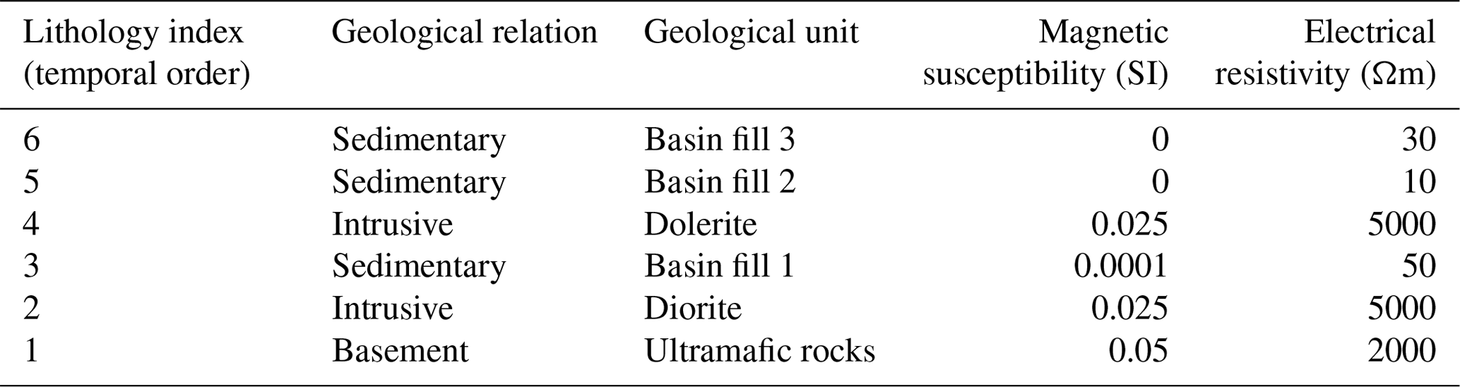
Table 1Stratigraphic column showing geological topological relationships and average physical properties. Lithologies are indexed from 1 through 6 by order of genesis.
The synthetic case study that we use to test our workflow is built using a structural geological framework initially introduced in Pakyuz-Charrier et al. (2018). It presents geological features that reproduce field geological measurements from the Mansfield area (Victoria, Australia). The choice of resistivity and magnetic susceptibility values to populate the structural model was made to test the limits of this sequential, cooperative workflow and to show its potential to alleviate some of the limitations inherent to potential field and MT inversions. To this end, we have selected a part of the synthetic model where MT data is affected by 2D and 3D effects to challenge the workflow we propose. The objective of this exercise is to assess the workflow's efficacy to recover the sediment–basement interface. To this end, we rely on the magnetic inversion's sensitivity to magnetic susceptibility contrast to model the interface between highly susceptible units (basement) and rocks presenting little to no magnetic susceptibility (sedimentary units). The magnetic susceptibility model we use consists of 2D structures.
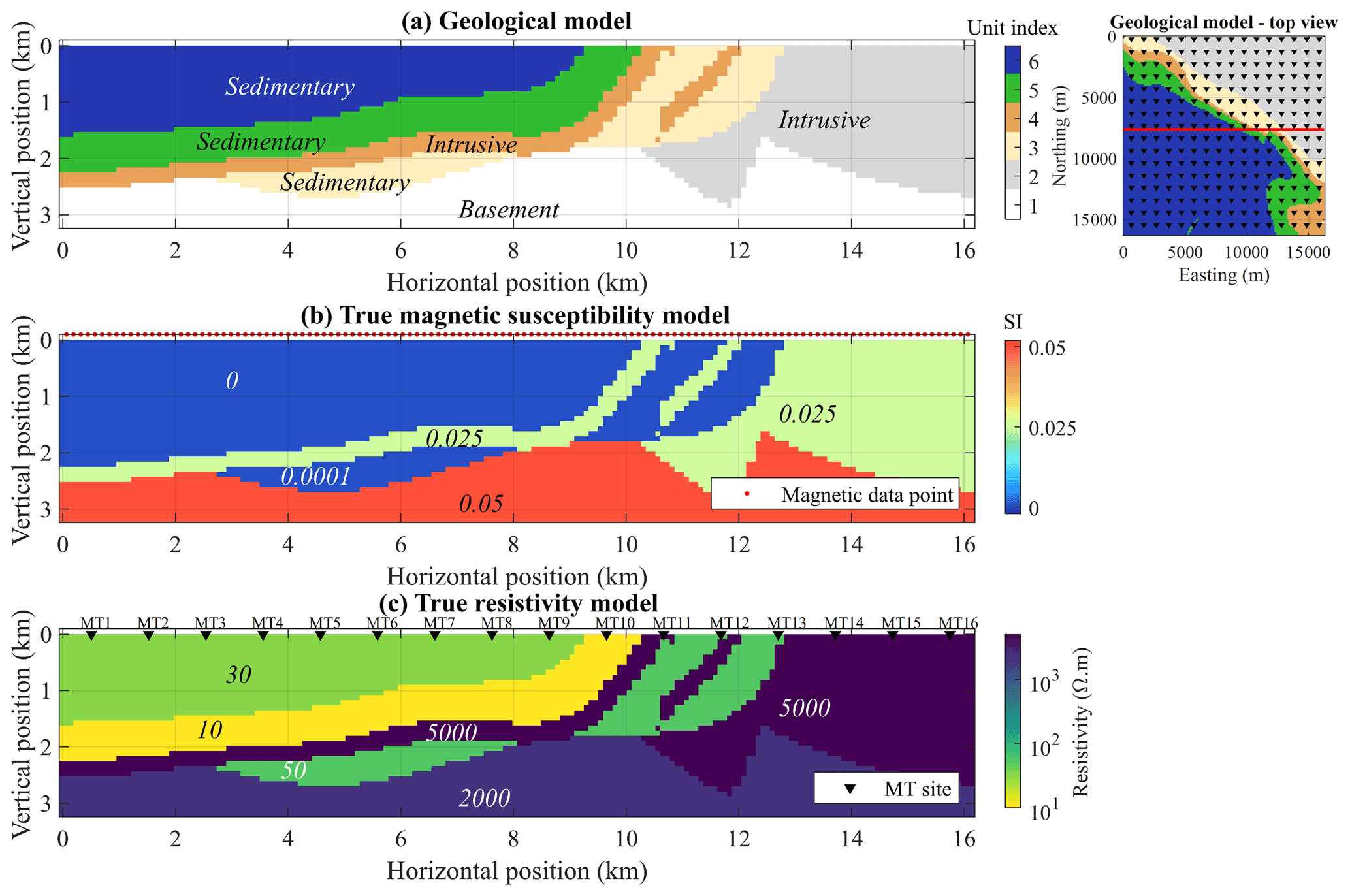
Figure 2(a) True geological model, (b) true magnetic susceptibility model and (c) true resistivity model with the simulated MT acquisition setup geometry in the top-left corner where triangles represent MT sites. The red dots in (b) represent the 2D magnetic data line; MT sites are marked in (c). The inset in the top-right corner shows a top view of the model with the magnetic data line in red and MT sites as triangles.
3.1 Survey setup
The structural geological model was derived from foliations and contact points using the Geomodeller® software (Calcagno et al., 2008; Guillen et al., 2008; Lajaunie et al., 1997). It is constituted of a sedimentary syncline abutting a faulted contact with a folded basement. The model's complexity was increased with the addition of a fault and an ultramafic intrusion. Details about the original 3D geological model are provided in Pakyuz-Charrier et al. (2018b). Here, we increase the maximum depth of the model to 3150 m and add padding in both horizontal directions. Figure 2a shows the non-padded 2D section extracted from the reference 3D geological model.
We assign magnetic susceptibility in the model considering non-magnetic sedimentary rocks in the basin units (lithologies 3, 5 and 6 in Table 1) and literature values (see Lampinen et al., 2016) to dolerite (lithology 4), diorite (lithology 2) and ultramafic rocks (lithology 1). We assign electrical resistivities assuming relatively conductive sedimentary rocks and resistive basement and intrusive formations. Resistivities in sedimentary rocks might vary by orders of magnitude and mainly depend on porosity, which is linked to the degree of compaction and the type of lithology and the salinity of pore fluid (Evans et al., 2012). The three sedimentary layers are assigned different resistivity values of 30, 10 and 50 Ωm for basin fill 3, 2 and 1, respectively (see Table 1), with basement being the oldest and deepest formation. Metamorphic and intrusive rocks as found in the crust generally present high resistivities (Evans et al., 2012). In what follows, we model data located along the line shown in Fig. 2, simulating the modelling magnetic data along a 2D profile (using a 3D mesh and a 3D forward solver), while considering 3D MT data. The modelled rock units and their petrophysical properties are given in Table 1. The true geological magnetic susceptibility and resistivity models are shown in Fig. 2.
3.2 Simulation of geophysical data
3.2.1 Magnetic data
The core 2D model is discretised into = 1 × 128 × 36 rectangular prisms of dimensions equal to 127 × 127 × 90 m3. We generate one magnetic datum (reduced to pole magnetic intensity) per cell along the horizontal axis, leading to 128 data points. To account for lateral effects, we add padding cells in both horizontal directions so that the padded model covers an horizontal area of 49 073 × 72 656 m2. The reference magnetic susceptibility model used for forward data computation is shown in Fig. 2.
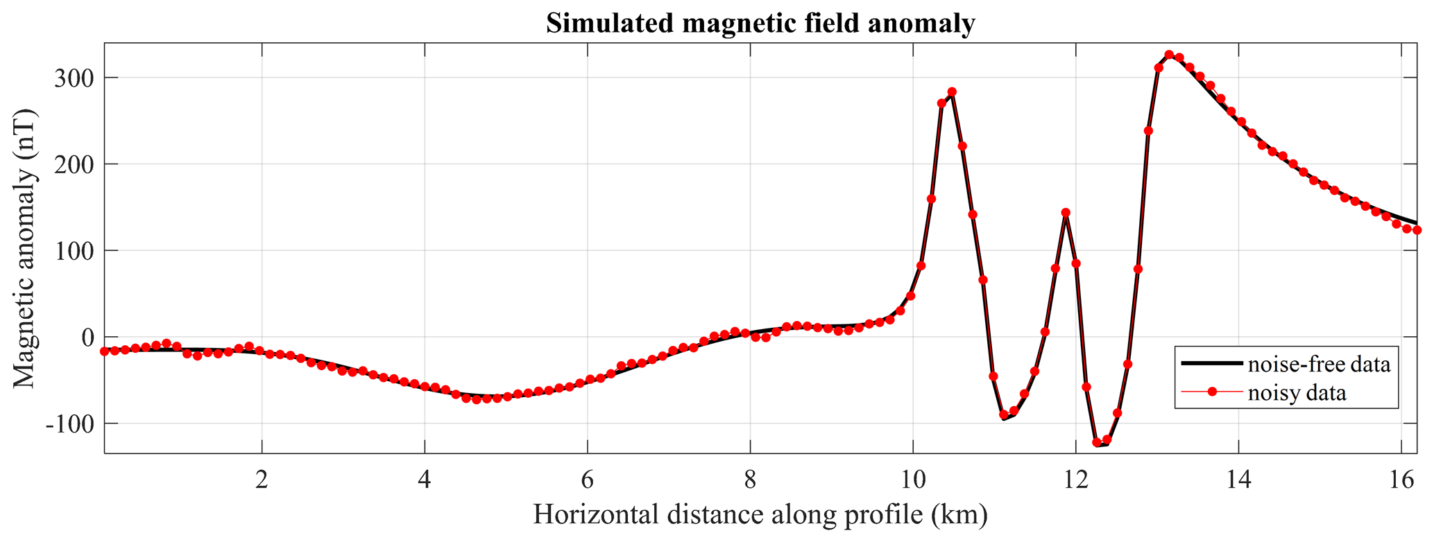
Airborne magnetic data are simulated for a fixed-wing aircraft flying at an altitude of 100 m above topography. The forward solver we use follows Bhattacharyya (1964) to model the total magnetic field anomaly. In this example, we model a magnetic field strength equal to 57 950 nT, reduced to the pole. It corresponds to the International Geomagnetic Reference Field for the Rawlinna station, Western Australia.
We add normally distributed noise with an amplitude equal to 4 % of the maximum amplitude of the data. We simulate noise contamination by adding noise sampled randomly from by a normal distribution characterised by a standard deviation of 3.8 nT and a mean value of 0 nT. For the simulation of geological “noise”, we then apply a Gaussian filter to such random noise to obtain spatially correlated values. The uncontaminated and noisy data are shown in Fig. 3. For the inversion, the objective data misfit is set accordingly with the estimated noise level.
3.2.2 MT data
The synthetic MT data is computed using the complete 3D resistivity model derived from the 3D geological model. The 3D resistivity model and the MT responses can be found online (Giraud and Seillé 2022). The core of the electrical conductivity model used the same discretisation as the magnetic susceptibility model (cells of dimension 127 × 127 × 90 m3 in the core of the model). More than 1000 km padding is added to the horizontal and vertical dimensions to satisfy the boundary conditions required by the forward solver. The final 3D mesh is discretised into = 160 × 160 × 62 cells. Relationships between geological units and electrical resistivities follow Table 1. The ModEM 3D forward modelling code (Egbert and Kelbert, 2012; Kelbert et al., 2014) is used to simulate the MT responses of this model. The MT responses are computed at 256 stations evenly spaced 1.016 km on a grid of 16 × 16 sites (see inset in Fig. 2). The frequencies we use span the 10 KHz to 0.01 Hz range, with six frequencies per decade, for a total of 37 frequencies; 5 % magnitude Gaussian white noise is added to the synthetic data before running the 1D inversions.
In the following subsections, we present the results of the modelling of synthetic MT data along a 2D section (see Fig. 2c) of the 3D resistivity volume, following the workflow proposed in Sect. 2. Along this section, 16 MT sites are used as mentioned above. We start with the modelling of MT data to derive constraints and prior information for the inversion of magnetic data.

Figure 4Example of posterior (a) response and (b) resistivity distributions for three MT sites MT1 (left), MT6 (middle) and MT10 (right), located along the profile as shown in Fig. 2. In (a) the phase tensor skewness β and ellipticity λ are shown. In (b) the change points (interface probability distribution), the cover–basement interface probability distribution pint and the sedimentary cover probability distribution psed are shown. Sites MT1 and MT6 are located in the basin, and site MT10 is located in the area most affected by 2D and 3D effects (see Fig. 2c for location). High probabilities in the model posterior distribution are represented by warm colours, and low probabilities are represented with cold colours. The dashed lines represent the 5th and the 95th percentiles of the model posterior distribution, and the black line represents the median of the model posterior distribution. The white line is the true 1D model extracted beneath the MT station.
3.3 One-dimensional Probabilistic inversion of MT data and derivation of cover–basement interface probabilities
We perform the 1D MT inversions of the 16 MT sounding independently using the 1D trans-dimensional Bayesian inversion described in Sect. 2.1. Synthetic data for three MT sites are shown in Fig. 4a. The phase tensor skewness β and ellipticity λ are also shown. We can observe that data that present large values of |β| (up to 10∘) and λ (up to 0.5), which is indicative of 2D or 3D effects (Caldwell et al., 2004), have been assigned larger uncertainties to compensate for these effects.
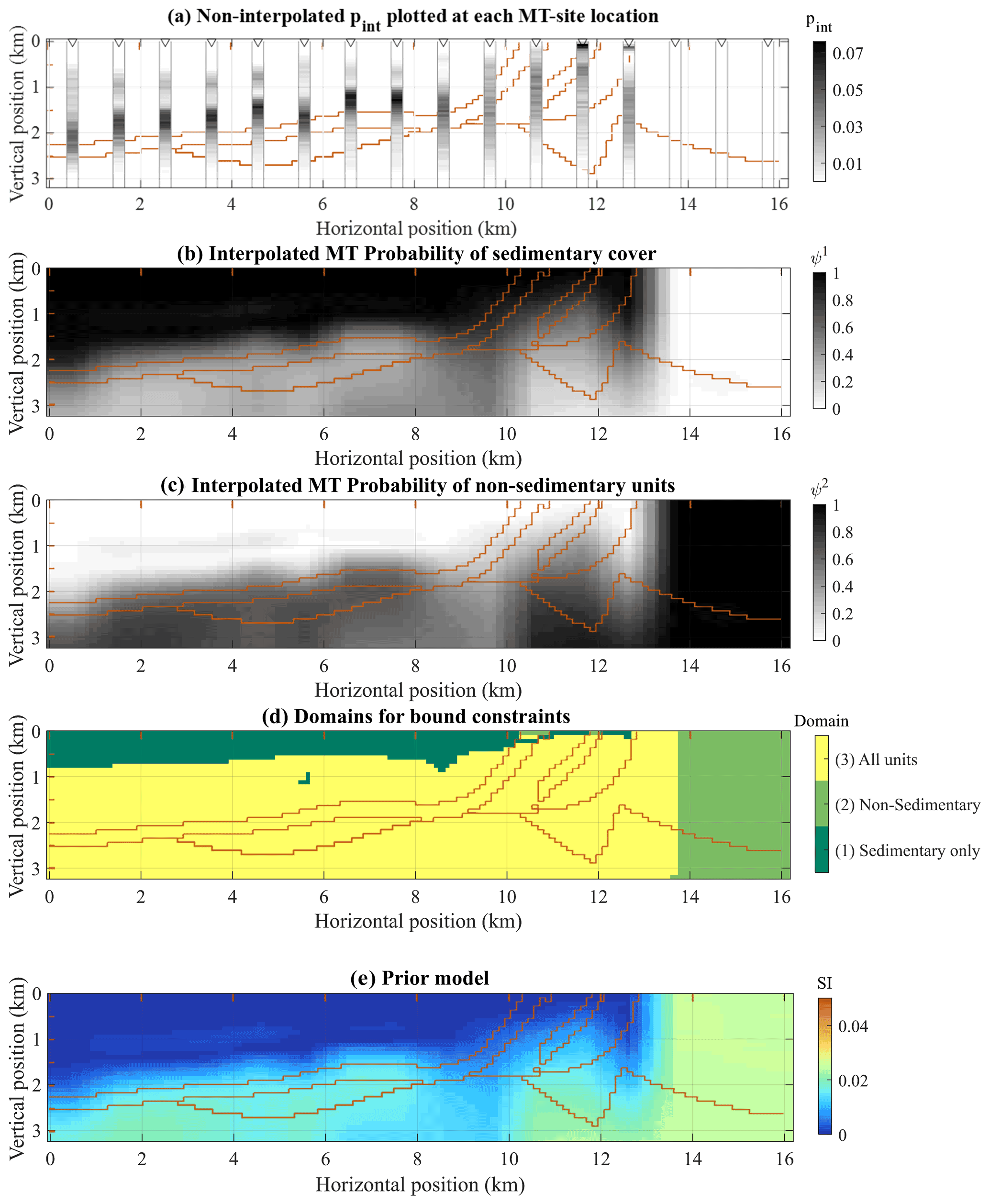
Figure 5Probability of interfaces between sedimentary cover pint and basements as recovered from MT inversion shown at the location of each MT site (a), interpolated probability of sedimentary cover, written as ψ1 (b), and non-sedimentary units, written as ψ2 (c), corresponding domains (d), and (e) the prior model from MT-derived rock unit probabilities and magnetic susceptibility rock units observed in the area. The location of the simulated MT sites is repeated in (a). The brown lines show the interfaces between geological units in the true model.
All the inversions ran using 60 Markov chains with 106 iterations each. For each chain, a burn-in period of 750 000 samples (75 % of the total) is applied to ensure convergence, after which we recorded 100 models equidistantly spaced within the chain. The model ensembles are then constituted by 6000 models for each MT site.
The model posterior distribution for three MT sites is shown in Fig. 4b. The interface probability within the posterior ensemble of 1D models is described by a change point histogram. From the posterior ensembles of models and interfaces, a cover–basement interface probability distribution pint is calculated independently for each MT site (see Fig. 4a). For this synthetic case, we assume a simple layer transition rule: transition from the sedimentary cover into the basement occurs when a layer L1 of resistivity ρ1<ρX is followed by a layer L2 of resistivity ρ2>ρX, with ρX = 200 Ωm. This value of ρX is chosen assuming a priori knowledge of the sediment resistivity in the area (which, for this synthetic case does not exceed 50 Ωm). Even without prior information, this assumption would be correct in most real cases, given that sediments are generally conductive, with resistivities ranging from 1 to 100 Ωm (Evans et al., 2012). The depths at which transitions that satisfy that rule occur form a 1D histogram, which we define as pint after normalisation (see Sect. 2.1 for details). Here, the use of more resistive threshold values does not have a significant effect on the calculation of pint. This process is applied to each model of the ensemble and allows the extractions of features of interest from the posterior model ensemble. If less than 0.1 % of all transitions observed in the ensemble present the feature defined earlier using ρX, we then assume that the transition is not observed. This situation occurs for MT sites MT14, MT15 and MT16 (see Fig. 2c for their location), where the intrusion outcrops and the transition into the basement are not detectable assuming the transition rule described above.
Figure 4 shows the interface probability and the cover–basement interface probability distribution pint for the three MT sites. For each MT site and at all depths, the probability of being in the presence of sediments, psed (defined as , Pint being the cumulative distribution function of the interface probability distribution pint; see Sect. 2.1), is calculated for all depths. Figure 5b shows psed for each location along the profile. We observe that MT sites located in areas affected by significant 2D and 3D effects, such as MT10 (see Figs. 2c, 4b and 5b), will have assigned larger uncertainties prior to the inversion. This will translate in the model posterior distribution as a relatively flat cover basement interface probability distribution pint and therefore a sediment probability distribution psed relatively uninformative for the magnetic constrained inversion.
3.4 Deriving constraints for magnetic inversion
3.4.1 Bound constraints
Starting from pint values calculated for each MT site, we interpolate psed from MT onto the mesh used for magnetic data inversion. In this synthetic example, we use a linear interpolation scheme. The interpolated probabilities from MT are shown in Fig. 5.
The interpolated probabilities pbsmt are used to define domains for the application of bound constraints during magnetic data inversion. The domains are derived from MT probabilities as introduced in Sect. 2.3. We divide the model into areas where the allowed magnetic susceptibility ranges correspond to rock units with probabilities superior to zero. In this example, we complement information from MT inversions with the assumption that dolerite outcrops and is mapped accurately at surface level (unit 4, intrusive; see Table 1 and Fig. 2). Using this, we only adjust the domains for the corresponding few model cells at surface level at two locations where outcrops are known based on the availability of a geological map. The domains for the bound constraints we obtain are shown in Fig. 5d, with domains 1 and 2 indicating parts of the model where MT inversion suggests a single rock unit. This means that in the corresponding model cells, a single interval will be used in the definition of the bound constraints, while intervals corresponding to two rock units (i.e. basement and sediments) will be used otherwise. The intervals we use are as follows:
-
domain 1 (sediments only): [−0.0001, 0.0002] SI;
-
domain 2 (non-sediment units only): [0.024 0.055] SI;
-
domain 3 (sediments and non-sediment units): [−0.0001, 0.0002] ∪ [0.024 0.055] SI.
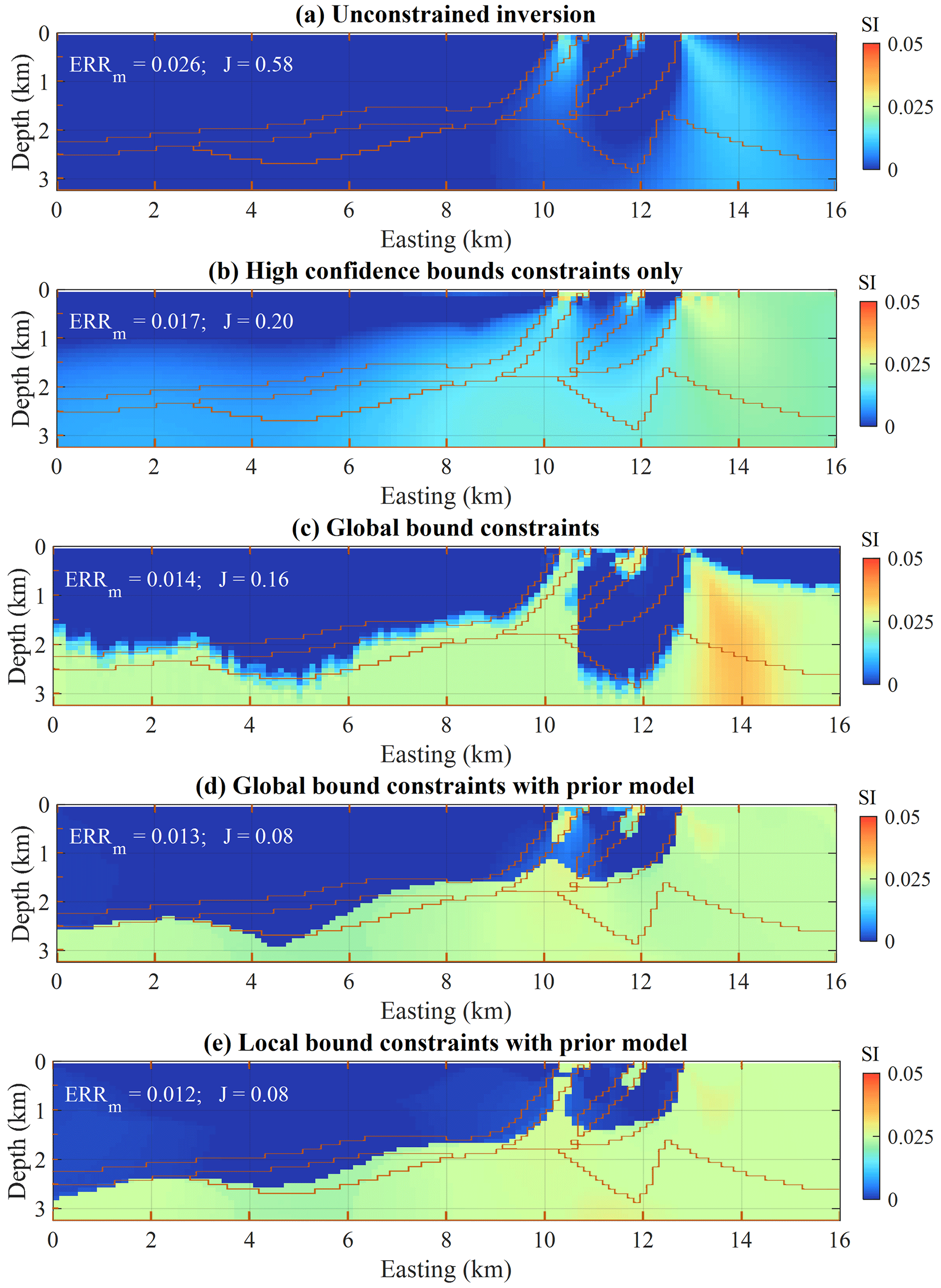
Figure 6Inversion results for the different scenarios tested. Cases (a) through (e) correspond to inversions using prior information and constraints summarised in Table 2.
3.4.2 Prior model and constraints from MT probabilities
The prior model for magnetic inversion is obtained using the MT-derived rock unit probabilities (Fig. 5b, c) and the magnetic susceptibility of the rock units given in Table 1. We proceed in the same spirit as Giraud et al., (2017), who calculate the mathematical expectation from probabilistic geological modelling to obtain a starting model for least-squares inversion. Here, we propose a different approach and combine information from the intervals with MT probabilities as follows. For the ith model cell, we have
We remind that is the probability of the jth rock unit in the ith model cell and that L is the number of rock units. We chose to use ai,j, the lower bound for each rock unit (or group of rock units), as it constitutes the most conservative assumption about magnetic susceptibility from the range of plausible magnetic susceptibilities. The resulting prior model is shown in Fig. 5e.
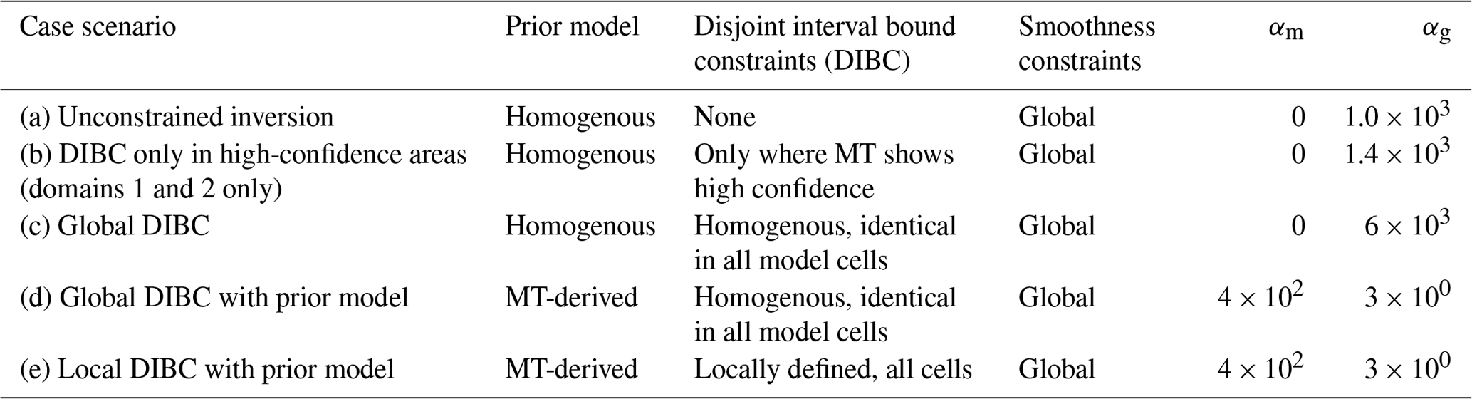
Table 2Scenarios tested for the utilisation of MT-derived information in magnetic data inversion. “High confidence” refers to the case where constraints are applied only to models cells with MT-derived rock unit probabilities equal to 1.
3.5 Inversion of magnetic data and uncertainty analysis
In this section, we study the influence of MT-derived prior information onto magnetic inversion and estimate the related reduction of interpretation uncertainty. In what follows, we consider that the prediction from MT can be considered with “high confidence” when the probability of one of the units is predicted with a probability of 1. We perform inversions for six cases, consisting of the following scenarios.
- a.
Unconstrained inversion. We assume no prior geological, petrophysical, or MT information; a homogenous prior model populated with magnetic susceptibility of 0 SI is used; no bound constraints are applied; and smoothness constraints are applied globally.
- b.
High-confidence bound constraints only. We assume knowledge of only domains 1 and 2 derived by MT (a single unit with 100 % confidence) to inform DIBC and that no probabilistic information is available elsewhere, DIBC are applied only in domain 1 and 2, a homogenous prior model populated with magnetic susceptibility of 0 SI is used, and smoothness constraints are applied globally.
- c.
Global bound constraints. We assume knowledge of the magnetic susceptibility of units that may be present in the area without MT or geological information, DIBC allowing all units everywhere in the model are applied, a homogenous prior model populated with magnetic susceptibility of 0 SI is used, and smoothness constraints are applied globally.
- d.
Global bound constraints with prior model. We assume knowledge of a prior model derived from MT but with a lack of probabilistic information, DIBC allowing all units everywhere in the model are applied, a prior model derived from MT prior information is used, and smoothness constraints are applied globally.
- e.
Local bound constraints with prior model. We assume knowledge of a prior model derived from probabilistic MT information to derive spatially varying DIBC, a prior model derived from MT prior information is used, DIBC are applied locally using information from MT, and smoothness constraints are applied globally.
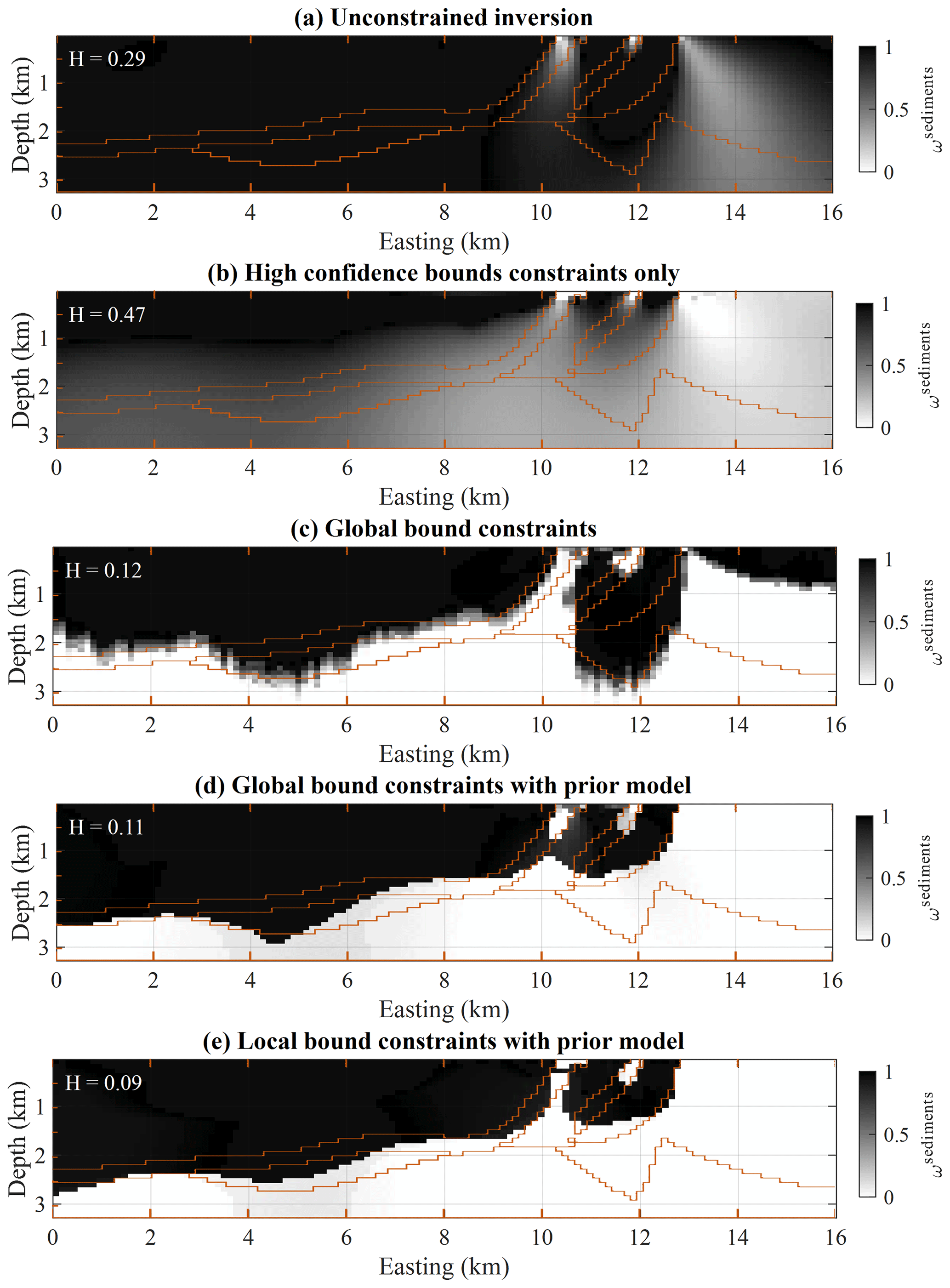
Figure 7Membership values for the non-magnetic lithologies. Cases (a) through (e) correspond to inversions using prior information and constraints summarised in Table 2. The brown lines materialise the interfaces between geological units in the true model. H refers to the information entropy of the model (Eq. 11).
The different scenarios tested in the synthetic example are summarised in Table 2. The corresponding inversion results are shown in Fig. 6. We note that magnetic susceptibility models shown in this section are equivalent from the magnetic data inversion point of view as they present a similar data misfit, which we assume to be acceptable when it is of the same magnitude as the estimated noise in the data.
Table 3Metrics calculated for the assessment of inverted models for cases (a)–(e).
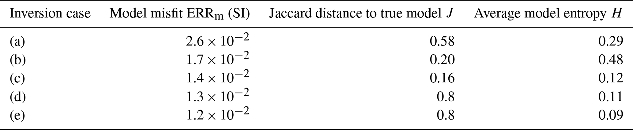
We complement the calculation of ERRm and J (see values in Fig. 6) with a membership analysis following Eq. (10) as a measure of interpretation uncertainty. The resulting membership values are shown in Fig. 7, where we added the values of the inverted model's information entropy H (Eq. 11). The values of metrics shown in Figs. 6 and 7 are summarised in Table 3.
A visual comparison of the membership values in Fig. 7e and e with the MT-derived domains (Fig. 5d) indicates good consistency with MT domains (1) and (2) (single rock units inferred). It also shows that the proposed workflow has the capability to improve the recovery of the sedimentary cover thickness significantly when compared to cases that do not use MT-derived DIBC across the entire model (Fig. 7a–c).
Two main observations can be made from the results shown in Figs. 6, 7 and Table 3. First, the use of DIBC at all locations of the model reduces interpretation ambiguity (lower H value for cases c–e). Second, the use of MT-derived DIBC produces models closer to the causative model by reducing both the model misfit ERRm and Jaccard distance (cases b and e). This supports qualitative interpretation of Figs. 6 and 7, pointing to the conclusion that exploiting probabilistic information to derive constraints for magnetic data reduces model misfit while supporting geological interpretability.
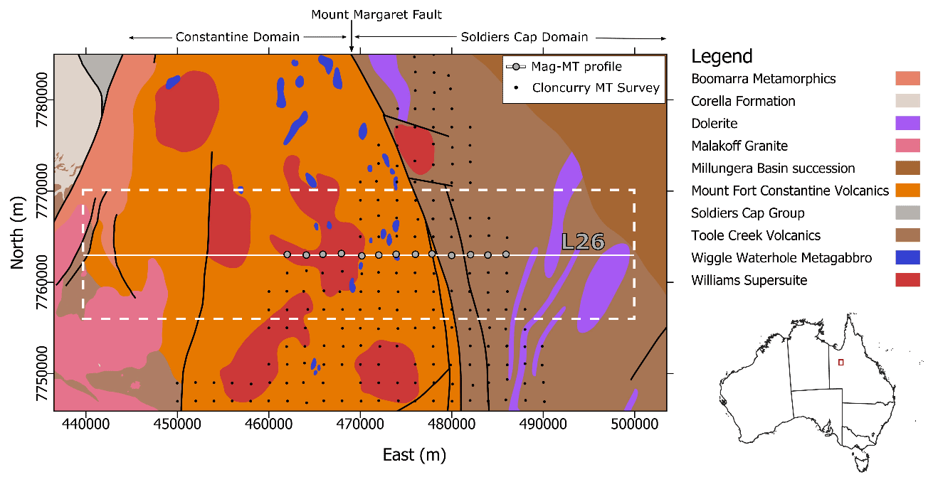
Figure 8Interpreted solid geological map of the area (Dhnaram and Greenwood, 2013). The small dots are the MT sites of the Cloncurry MT survey. The red line is the profile used in this study, and the red dots are the MT sites associated to this profile. The Constantine domain to the west and the Soldiers Cap domain to the east are separated by the Mount Margaret fault. The dashed red line delineates the area we focus on.
We propose an application example illustrating potential utilisations of the proposed sequential inversion workflow in the Cloncurry district (Queensland, Australia; see Fig. 8). Using observations made in the synthetic case, our aim here is to integrate MT with magnetic data inversion using the case relying on MT-derived DIBC with a homogenous starting model and smoothing constraints.
We use existing results of the depth to basement derived using MT within a probabilistic workflow (Seillé et al., 2021) in an area of the Cloncurry district. These results are used to constrain the magnetic inversion.
4.1 Geoscientific context and area of interest
The depth to basement interface probability used to constrain the magnetic inversion was derived as part of a previous study using a similar workflow as presented in Sects. 2.1 and 3.3, details about the survey can be found in Seillé et al.(2021) and are summarised in what follows. The study consisted of modelling the full Cloncurry MT dataset using 1D probabilistic inversions. For each MT site, the cover–basement interface probability distribution pint was extracted from the inversion model ensembles. In this area, the threshold used to discriminate between sedimentary and basement rocks was set to 800 Ωm due to the presence of relatively resistive sediments. The set of 1D cover–basement interface probability distribution pint was then interpolated spatially across the survey area using the Bayesian estimate fusion algorithm of Visser and Markov (2019). This algorithm generates an ensemble of 2D surfaces, given discrete input estimates of the location of an interface. In that study, two types of depth to basement estimates were combined: the cover–basement interface probability distribution pint derived from the MT, and the depth to basement estimated from drill hole data. In total, 457 MT sites and 540 drill hole estimations are combined. Significant lateral variations are allowed during the interpolation using the fault traces indicated by structural geological data, defining areas where basement discontinuities are expected (at the location of faults). A relaxation of the spatial continuity between estimates located on different sides of a given fault is encouraged, allowing for discontinuities in the interpolated 2D surfaces (Visser and Markov, 2019). These faults are assumed to be vertical, which is a valid assumption given the near-vertical behaviour of the main faults in the area (Austin and Blenkinsop, 2008; Case et al., 2018). The combination of estimates coming from different sources of information in this form permitted us to calculate a probabilistic depth to basement interface across the survey area.
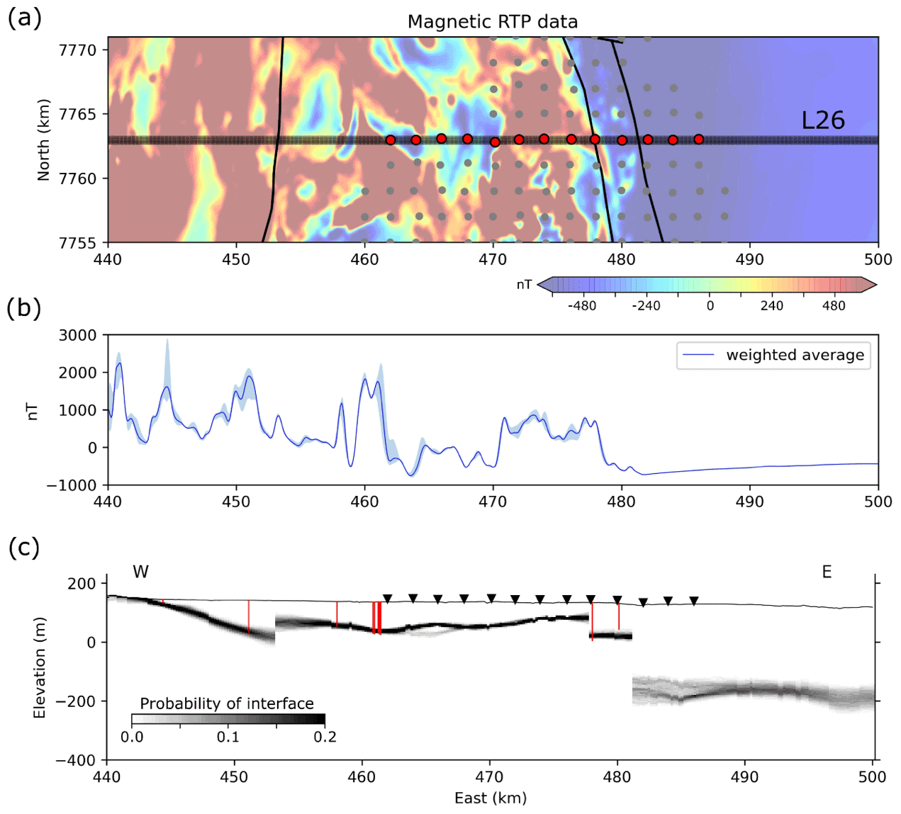
Figure 9Data preparation. (a) Map view of the data in the region of interest. The greyed-out area corresponds to the zone considered for the averaging of the magnetic data. Red points are MT soundings considered in this study. Grey circles are other MT soundings not used in this study. Panel (b) shows data for magnetic inversion (solid line) and the envelope of the data from the 800 m band around L26 (light blue shading). The shades of blue represent the weight assigned to the data points in the calculation of the average: the lighter the shade, the lower the weight. (c) Cover–basement interface probability pint (Seillé et al., 2021). Red lines are the drill holes, and their bottoms represent the intersection with the basement. The drill holes plotted are projected at a distance up to 800 m away from the profile.
In this study, we focus on a 2D profile (L26; see location on map in Fig. 8a) and invert the corresponding magnetic data extracted from the anomaly map shown in Fig. 9a and b. The choice of an east–west-oriented profile is motivated by the north–south orientation of the main structures in the area and by the geological features that the known geology and the geophysical measurements suggest. The profile is nearly perpendicular to these structures, making it suitable for use within a 2D inversion scheme. It crosses the north–south-oriented Mount Margaret fault, which is thought to belong to the northern part of the regional Cloncurry fault structure, a major crustal boundary that runs north–south over the Mount Isa province (Austin and Blenkinsop, 2008; Blenkinsop, 2008). This boundary separates two major Paleoproterozoic sedimentary sequences (Austin and Blenkinsop, 2008). The geological modelling performed by Dhnaram and Greenwood (2013) also indicates that the Mount Margaret fault separates two distinct domains, the Constantine domain to the west and the Soldier Caps domain to the east. In our study area, the Constantine domain is covered by non-magnetic cover constituted of Mesozoic and Cenozoic sediments, lying on what is believed to be the Mount Fort Constantine volcanics, which is in some places intruded by the Williams Supersuite pluton. On the eastern side, the Soldier Caps domain is also covered by Mesozoic and Cenozoic sediments, and the basement is interpreted to be a succession of volcanic and metamorphic rocks (Dhnaram and Greenwood, 2013).
The depth to basement probabilistic surface derived by Seillé et al. (2021) along the E–W profile (see Fig. 9c) presents shallow basement depths in the western part of the profile (top basement at a depth of approximately 100 m, with some lateral variations). In the eastern part of the profile, the model indicates that a two-step fault system controls the thickening of the basin to the east. It reaches ∼ 350 m thickness in the eastern part. The depth to basement model along the profile shown in Fig. 9c is relatively well constrained by MT and the drill hole data used in the interpolation process. However, the interpolation method we used imposed spatial continuity between estimates. Due to the relatively large separation between soundings (2 km) and the sparsity of drill holes, it did not allow for the definition of small-scale depth to basement lateral variations. In contrast, magnetic data shown in Fig. 9a suggest that small-scale variations due to faults and other lateral discontinuities could exist.
In this work, we assume a non-magnetic sedimentary cover and a magnetic basement. In addition, we assume little to no remanent magnetisation and little to no self-demagnetisation. Important remanence and self-demagnetisation can be observed in the vicinity of magnetite-rich iron oxide, copper, and gold ore deposits (e.g. Anderson and Logan, 1992; Austin et al., 2013), but we consider there to be no indication of such features along L26. Further to this, we make this assumption for the sake of simplicity as the main object of this paper is the introduction of a new sequential inversion workflow and to show that it is applicable to field data.
Under these premises, the features the magnetic data presents can be exploited to improve the image of the cover–basement interface when integrated with prior information about the thickness of cover. In this context, magnetic data inversion constrained by MT performs multiple roles:
-
constraining the depth and extent of the magnetic anomalies and refine their geometry;
-
analysing the compatibility between the constraints derived from MT and the magnetic data and resolving some small-scale structures not defined by the MT constraints;
-
reducing the interpretation uncertainty of the cover–basement interface;
-
proposing new scenarios in relation to the composition of the basement (in terms of its magnetic susceptibility) and structure (through its lateral variations).
The depth of the cover–basement interface probability shown in Fig. 9c is used to derive the domains required by the spatially varying bound constraints used in magnetic inversion.
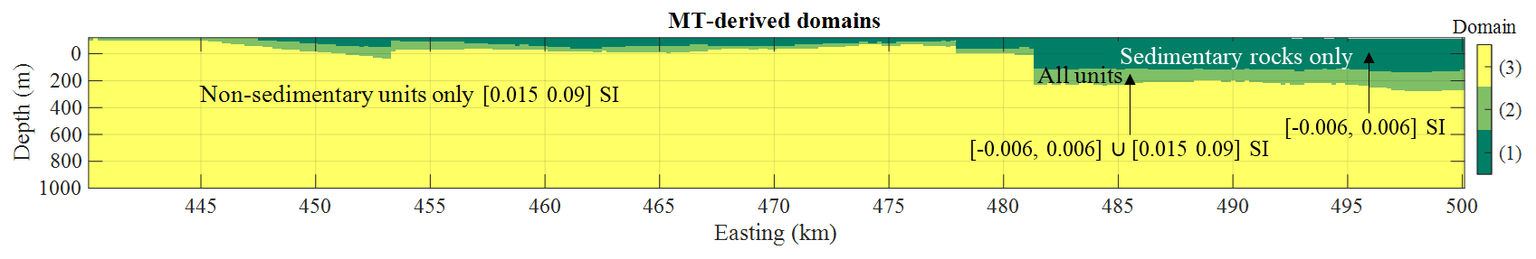
Figure 10MT-derived domains for cases with (i) sedimentary units only, (ii) sedimentary and non-sedimentary units and (iii) non-sedimentary units only. The magnetic susceptibilities for the different domains are also indicated.
Table 4Scenarios tested for the utilisation of MT-derived information in the field case and corresponding α weights used in the inversion.

4.2 Constrained magnetic data inversion
4.2.1 Magnetic data preparation and extraction of prior information
We use the gridded reduced-to-pole (RTP) magnetic data from the Geological Survey of Queensland shown in Fig. 9 (https://geoscience.data.qld.gov.au/dataset/ds000018/resource/91106497-d463-4b83-8b01-1c5539ab40b1, last access: 15 November 2022). Prior to the 2D inversion of the data along line L26, we manipulate and reformat the data. To account for variations in the measurements in the vicinity of the line, we extract data from a 800 m wide band around the profile (L26) (Fig. 9a), as shown in more detail in Fig. 9a. To obtain data corresponding to a 2D rectilinear profile, we then calculate the weighted average of this subset of the dataset by assigning weights inversely proportional to the square of the distance of the measurement to L26, as illustrated in Fig. 9b. The envelope of the data is obtained from the lower and upper limits observed within the band considered in the calculation of the weighted average. As a consequence, it reflects the variability of magnetic data perpendicularly to L26. Areas with departures from a narrow envelope may be indicative of zones where the 2D hypothesis made for inversion could be challenged.
We convert the interface probability shown in Fig. 9c into basement and sedimentary rock probabilities using the method described in Sects. 2.1 and 3.4.1. We assume that the sedimentary basin domain overlies the basement domain and derive the corresponding domains for the DIBC using the domain procedure described above. The resulting domains are shown in Fig. 10.
In what follows, we assume that sedimentary rocks have a low magnetic susceptibility comprised within the range [−0.006, 0.006] SI, while the basement units, mainly composed of volcanic sequences, are modelled to have higher magnetic susceptibilities within the interval [0.015, 0.09] SI. The intervals we use for domains 1, 2, and 3 are given as follows:
-
domain 1 (sediments only): [−0.006, 0.006] SI;
-
domain 2 (basement and sediments): [−0.006, 0.006] ∪ [0.015 0.09] SI;
-
domain 3 (basement only): [0.015, 0.09] SI.
Note that the lowest magnetic susceptibility values are negative (−0.006 SI).
4.2.2 Inversion setup and results
Similar to the synthetic model used in Sect. 3, padding cells were added in both horizontal directions. The resulting model covers a surface area defined by a rectangle of 157 km along the main profile axis and 50 km perpendicular to it. All inversions shown here were performed on a laptop computer using five threads on an Intel(R) Xeon(R) W-10855M CPU.
To examine the impact of different type of constraints, we first perform inversions using minimum prior information and successively increase the amount of prior information from unconstrained inversions by using MT-derived intervals for multiple-bound constraints. In the scenarios investigated here, we perform inversion using global smoothness constraints (Wg=I), global (i.e. uniformly applied) and local (i.e. spatially varying) DIBC. The inversions we run consist of the following cases:
-
constrained by global smoothness constraints,
-
constrained by global smoothness constraints with lower- and upper-bound constraints,
-
constrained by global smoothness constraints with global multiple-bound constraints,
-
constrained by global smoothness constraints with local DIBC defined from MT probabilities.
The constraints used in each case are summarised in Table 4.
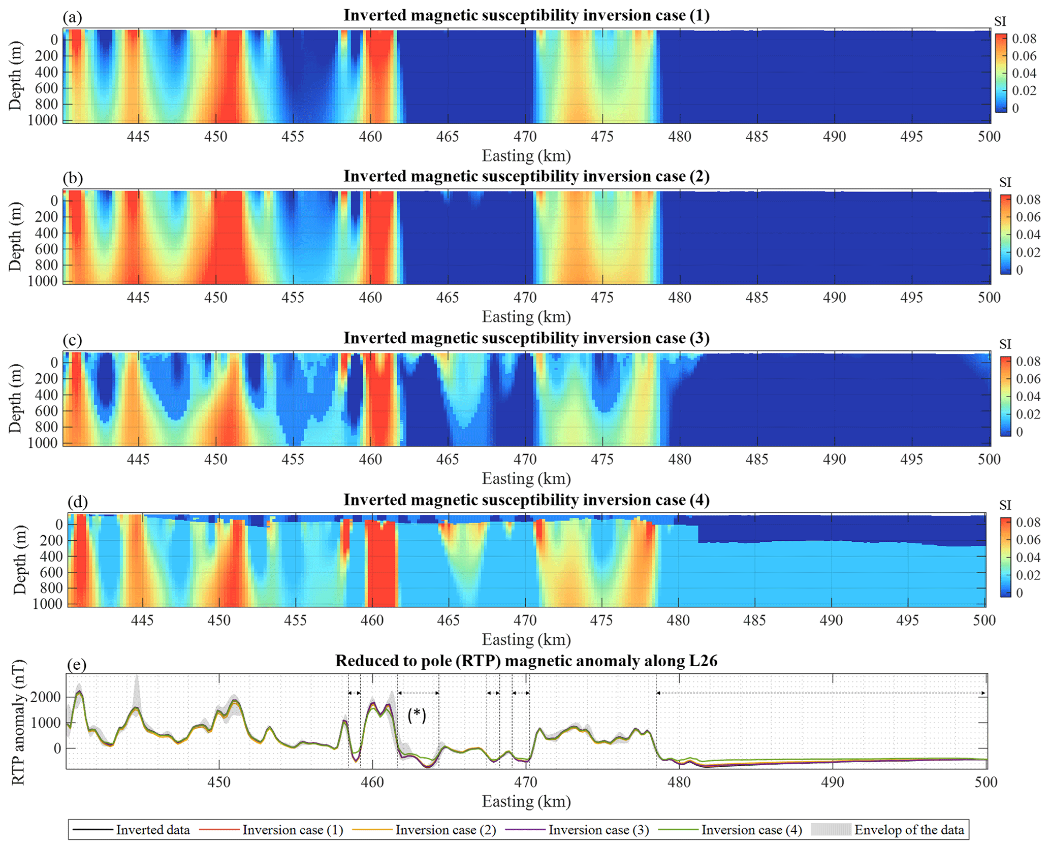
Figure 11Inversion results. Panels (a) through (d) correspond to inversion types (1) through (4) as per Table 4, respectively; panel (e) shows the data fit for the four inversions shown. The grey shading shows the amplitude of the data shown in Fig. 9 for calculating the weighted average of the inverted anomaly. The dashed lines mark the horizontal extension of areas where hypotheses made for magnetic inversion may be incompatible with the data.
Similarly to the synthetic case, we determine the value of αm and αg for each case using an L-curve analysis. This step is performed starting from a coarse model discretisation by doubling the cell size in each direction to save computation time, followed by fine tuning on the finer mesh. The results for inversion cases (1) through (4) are shown in Fig. 11.
The inversions reached a satisfactory data fit, with the exception of the constrained inversion 4 (see the data fit in Fig. 11e). In that case a significant underfit of the magnetic data is observed within certain areas, which points to an incompatibility between the magnetic data and the constraints applied. Four areas in the central part of the model are slightly underfit, as shown by double arrows between approximately 458 km and 470 km east. On the eastern part of the profile, from 479 km east to the most eastern part of the profile, an important underfit is observed, as marked by the rightmost double arrow in Fig. 11e. At this stage, this data misfit could indicate that the constraints used are not appropriate. This could be due to an inexact positioning of the structural constraints at depth or to a change in the petrophysical behaviour of the basement in certain areas, which would differently link the electrical properties of the depth to basement constraints to their magnetic properties We propose a fifth inversion case where we adjust the bounds manually to examine hypotheses relaxing the constraints derived by the combination of MT inversions and the magnetic susceptibility of rocks in the area.
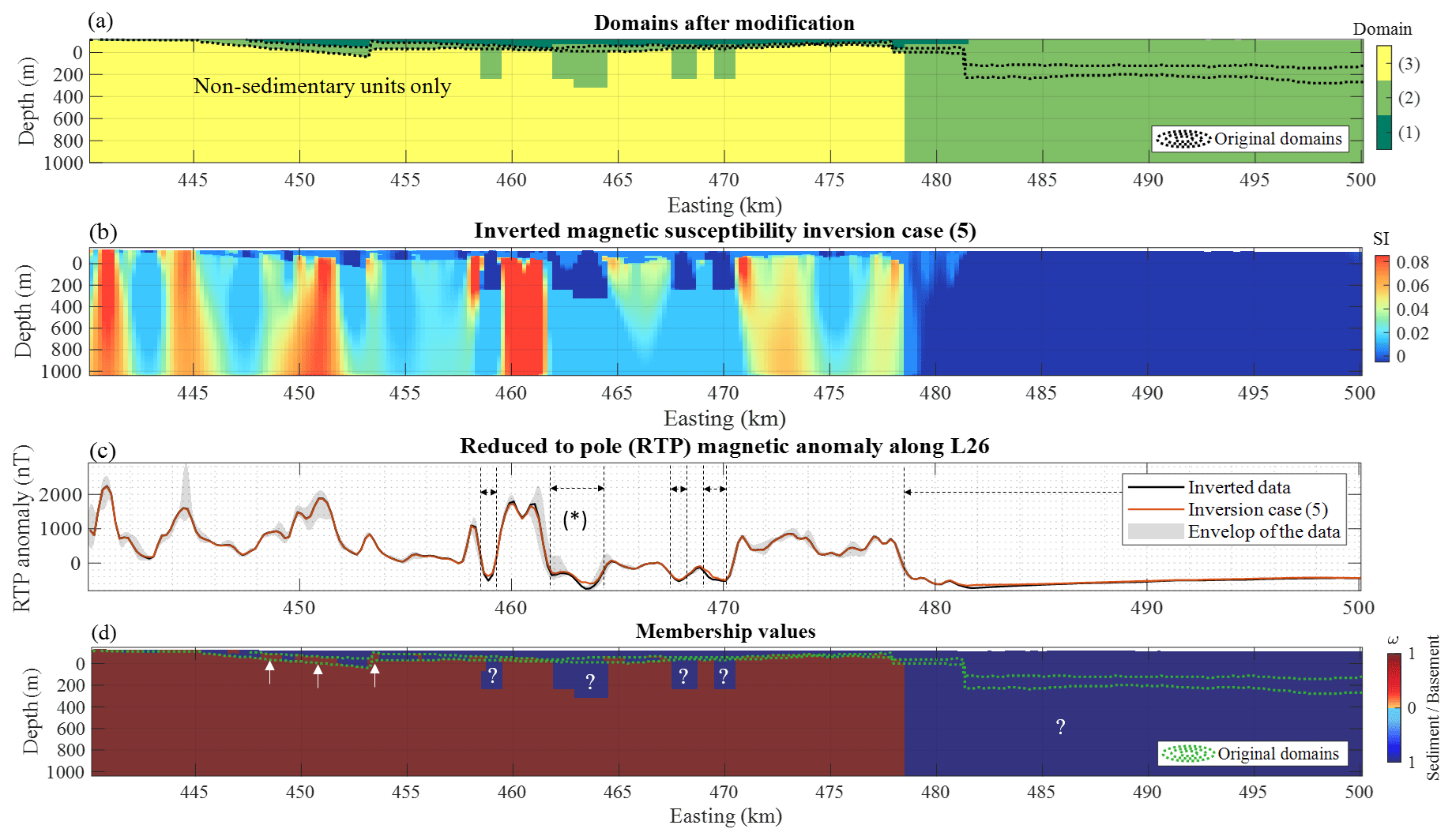
Figure 12(a) MT-derived domains adjusted following the adjustments suggested by magnetic data inversion, for domains with (1) sedimentary units only, (2) sedimentary and non-sedimentary units, and (3) non-sedimentary units only. Panel (b) is the inverted model for inversion case (5), and panel (c) is the inverted and field magnetic RTP data, with the horizontal extent of the locations where MT bounds are adjusted. Panel (d) shows the membership values to the sedimentary and basement units obtained using Eq. (10), overlaid with the original contours of MT-derived domains. In (c), the grey shading shows the envelope of the data shown in Fig. 9 for calculating the weighted average of the inverted anomaly.
From Fig. 11, we identify five main areas where hypotheses made for the utilisation of MT-derived domains need to be adjusted. In each case, the domain allowing sedimentary units may be deeper than expected or the basement may be less susceptible. We test the plausibility of such alternative scenarios by adapting the MT-derived domains by adjusting the domains. We increased the depth of the non-sedimentary (i.e. basement) units in the eastern part of the model and between the areas delimited by dashed lines in Fig. 11d. From a geological point of view, this corresponds to adjusting our working hypothesis to a case where rocks previously identified as basement only may be less susceptible than expected. The domains we use after adjustment are shown in Fig. 12a, and inversion results are shown in Fig. 12b and c, respectively. Figure 12d proposes an automated interpretation with membership values ω using Eq. (10); the question marks shown in Fig. 13d identify areas where the initial hypotheses have been revisited from a structural point of view by modifying the domains but may still require further investigation, such as the use of different interval bounds to simulate lateral petrophysical variations within the basement. This could be a way to assess the natural heterogeneity that can occur within basement units due to geological events still unaccounted for in the modelling. The arrows point to parts of the model where the basement constraints may be poorly resolved because they are located outside of the coverage of the MT stations and only constrained by few sparse drill hole estimates (Fig. 9a and c). We note that this possible interpretation needs to be taken with caution between approximately 462 and 464 km east, as marked by the asterisk sign (*) in Fig. 12e and c, because it corresponds to a zone of the study area where the assumption of a 2D model taken for the magnetic inversion might not hold. This is corroborated by visual inspection of the vicinity of L26 beyond the greyed-out area between 462 and 464 km east in Fig. 9a.
Beyond the possibility to review hypotheses made at earlier stages of the workflow, we get insights into the structure and magnetic susceptibility of the basement. While electrical conductivity and magnetic susceptibility may be sensitive to changes in rock type, there are scenarios where they exhibit differing sensitivity to texture and grain properties, respectively. For instance, metamorphism and alteration might affect electrical conductivity and magnetic susceptibility differently (Clark, 2014; Dentith et al., 2020). Under these circumstances, our results can provide indications about plausible geological processes given sufficient prior geological information about the deformation history.
4.3 Interpretation
From a multi-physics modelling point of view, the results presented in the previous section show a general agreement between the MT-derived constraints and the magnetic data. However, the results also show incompatibilities in a few parts of the model. We identified two major areas where incompatibility occurs:
-
a smaller inconsistent area in the western part of the survey,
-
a large inconsistent area east of the Mount Margaret fault.
We interpret these incongruities as being mainly due to the different sensitivities of the two geophysical methods to different geological features and to the petrophysical variability of the basement in the area.
The greater depth extent of some of the lower magnetic susceptibility zones required by the magnetic data in the western part of the survey suggests that the depth to magnetic source is greater than suggested by the constraints. Adjustments to the constraints allowed a better data fit. A low magnetic response between 460 and 470 km east (Fig. 9) is assumed to be the consequence of low magnetic susceptibility contrasts and is interpreted to be granitic intrusions of the Williams Supersuite (Dhnaram and Greenwood, 2013). The presence of such intrusions offers a plausible explanation for the discrepancies between the magnetic and MT modelling. On the one hand, MT data modelling might not able to distinguish between an electrically resistive basement and an electrically resistive intrusion, while magnetic data modelling could not distinguish between the non-magnetic cover and a non-magnetic intrusion. On the other hand, magnetic data inversion can differentiate the low-susceptibility intrusion from the higher-susceptibility volcanic rocks, and the MT data are sensitive to the basal cover interface above both the volcanic rock and the intrusion. The constrained inversion permits detection of the lateral extent of the intrusion while estimating cover thickness. While detailed modelling of higher-resolution data would be required to refine the geometry of these intrusive bodies, our modelling suggests that the intrusion could be modelled as several smaller intrusions.
East of the Mount Margaret fault, the incompatibility between the original MT-derived constraints and the magnetic data points to regional-scale structures. Drill hole observations indicating basement do not exceed 350 m depth. If we assume a high-susceptibility basement, which is common to the whole area (Dhnaram and Greenwood, 2013), the magnetic model requires a very thick non-magnetic cover layer to reconcile the data that are incompatible with our geological knowledge of the area. In that case, we need to reconsider our definition of the basement. The north-trending Mount Margaret fault (see Fig. 8) separates two geological domains exhibiting different basement characteristics. East of the fault is the Soldiers Cap domain, which is predominantly composed of non-magnetic volcanic rocks. By relaxing the geological model constraints in that part of the model, both the sedimentary and non-sedimentary units are allowed (Fig. 10a), and we can thus satisfactorily fit the data. The necessity of considering non-magnetic volcanic rocks in the Soldier Caps domain is in agreement with the magnetic modelling performed by Dhnaram and Greenwood (2013).
We have presented a workflow for sequential joint modelling of geophysical data and applied it to synthetic and field measurements. In this study we used constraints in the form of interface probabilities derived from a probabilistic workflow driven by MT data, but it is general in nature and is not limited to a particular geological or geophysical modelling method to generate the inputs. This has allowed us to report the utilisation of the ADMM algorithm to constrain magnetic data inversion using disjoint interval bound constraints for the first time.
This workflow presents several advantages. It is computationally inexpensive via the use of standalone inversions. The inversion of the MT dataset used to derive the constraints is performed only once. Following this, a series of constrained magnetic inversions is run to test different geophysical and petrophysical hypotheses. It shows the example of a fast and flexible approach to test different structural and petrophysical assumptions while modelling data sensitive to different physical parameters. It allows us to focus the modelling efforts on survey-specific features (anomalies, geological structures) when appropriate petrophysical information is available. However, as with generalisable methods, strengths become limitations under certain circumstances. For instance, in the case of MT and magnetic data inversions as proposed in this work, the electrical resistivity and magnetic susceptibility for the rock types of interest is dependent on a range of factors and processes (such as porosity, permeability, rock alteration) such that their correlation may be case dependent (see Dentith et al., 2020; Dentith and Mudge, 2014). While we may surmise that it remains reasonable to assume the existence of such correlation in hard rock scenarios, it may not always hold in basin environments. For example, one can easily think of a basin exploration case where electrical resistivity increases rapidly with increasing hydrocarbon concentration in reservoirs, while changes in magnetic susceptibility might make the use of magnetic data inversion redundant. In such cases, property pairings other than magnetic susceptibility and resistivity could be considered for variables such as electrical resistivity and seismic attributes (see examples in Le et al., 2016, and Tveit et al., 2020, who use seismic inversion to extract prior information for CSEM inversion). Further to this, the utilisation of magnetic data inversion for the deeper part of the crust is limited to depths shallower than the Curie point (typically from approximately 10 km to a few tens of kilometres under continents). For deeper imaging of the crust, the workflow we propose may be suited to the utilisation of gravity data with MT.
An assumption that is worth examining is whether the study area is adequately represented by two geological domains. In the cases we investigated, these domains are defined by the probability of observing only two rock classes (basement and non-basement). While this assumption reduces the risk of misinterpretation as no hypotheses are made to distinguish between different sedimentary units or rocks of different nature in the basement, it also then limits the interpretations that can be made from the results presented. We expect that if the rock units present discriminative features, i.e. distinctive magnetic susceptibility and resistivities (or other properties depending on the geophysical techniques considered), several rock types can be considered in the modelling. Such discriminative aspects of the petrophysics need to be ascertained while defining the number of distinctive domains that may be present in the study area. Ideally, robust petrophysical data are available given the strong constraint that these domains may impart on inversion. However, in the absence of petrophysical data or the number and character of geological domains, literature values or broad intervals can be used to define constraints. In these cases, the magnitude of the data misfit can inform us as to whether a proposed number of domains or magnetic susceptibility ranges are plausible, driving data acquisition or refinement of the conceptual geological model. Methods that exploit this approach remain to be investigated further in future case studies.
The application case is performed in 2D to illustrate the workflow. Extending the presented work to large-scale problems in 3D is straightforward as the inversion methods employed in this study are designed for 3D modelling. The 1D MT modelling and interpolation schemes present excellent scalability. The Tomofast-x engine (Giraud et al., 2021b; Ogarko et al., 2021b) is implemented using 3D grids. It presents good scalability and it offers the possibility to reduce the size of the computation domain to save memory when calculating the sensitivity matrix in the same fashion as Èuma et al. (2012) and Èuma and Zhdanov (2014) for large-scale potential field data modelling. Ongoing developments on Tomofast-x comprise the application of wavelet compression operators to accelerate the inversion in the same way as Li and Oldenburg (2003) and Martin et al. (2013) while maintaining a sufficiently low modelling error and developing joint inversions using the DIBC.
Another straightforward extension of the workflow is the use of gravity data simultaneously with (or instead of) magnetic data since it is already implemented in Tomofast-x (Giraud et al., 2021b). Giraud et al. (2021c) presented a synthetic MT-constrained gravity inversion using a similar workflow to the one presented here. This would be of particular interest in the Cloncurry region (Queensland, Australia), where, for instance, Moorkamp (2021) recently investigated the joint inversion of gravity and MT data, and where our workflow could be applied using the MT modelling results of Seillé et al. (2021).
From a geophysical point of view, magnetic inversion is affected by the non-uniqueness of the solution to the inverse potential field problem despite prior information and constraints being used. The workflow could be improved by using a series of models representative of the geological archetypes that can be derived from the ensembles of 1D MT models. Geological archetypes are distinctly different structural configurations (or topologies) that plausibly exist for a given location with available data (Pakyuz-Charrier et al., 2019, Wellmann and Caumon, 2018). Identification of the archetypes could be achieved from the ensemble of geological model realisations in the same spirit as Pakyuz-Charrier et al. (2019), who use a Monte Carlo approach to generate a range of topologies that are then examined for distinct clusters representing the archetypes.
From a methodological point of view, it could be argued that simultaneous joint geophysical inversion combining structural and petrophysical constraints might outperform the workflow we propose here. However, this would make the modelling process more demanding when combined with limitations based on cases where determining the causative relationships between petrophysics supporting joint approaches poses a challenge. The workflow we propose here presents a few advantages over a joint inversion scheme, in the sense that it does not require both datasets to be inverted simultaneously under a defined set of petrophysical and/or structural constraints. As the time required to run a joint inversion is limited by the running time of the more computationally expensive technique, it can limit the range of tests to be performed. In this study, we could rapidly run many 2D constrained magnetic inversions, even if the 1D probabilistic inversions of the MT data (and posterior fusion) required significantly longer running times compared to the 2D constrained magnetic inversion. This point would be particularly relevant in the case of large 3D datasets. This approach may represent a step in the modelling workflow that is useful to explore, understand and refine structural and petrophysical relationships between different physical parameters before undertaking more demanding joint inversions.
In the field application case presented here, the probabilistic depth to basement is derived assuming lateral continuity of the depth to basement estimates at a large scale, not accounting for small-scale lateral variations. Thus, uncertainty in the depth to the basement may be underestimated at some locations, in particular in between MT sites as shallow depths. In such cases, the existence of incompatibilities between MT-derived constraints and the magnetic data might require reconsidering the spatial continuity assumptions taken during the calculation of the probabilistic depth to basement surface. Extensions of this work may be devised to alleviate some of the limitations of the workflow. For instance, magnetic susceptibility from the inversion of magnetic data could be mapped back to a resistivity model to calculate forward MT data for validation (dashed line in Fig. 1) or to constrain the next cycle of MT inversions in the case the workflow is extended to cooperative joint inversion. It would also be straightforward to use to a level set inversion that can consider an arbitrary number of geological units (e.g. Giraud et al., 2021a) using MT modelling as a source of prior information and constraints. We have used hard bounds using the ADMM algorithm, which can easily be complemented or replaced by the use of multi-modal petrophysical distributions as available in Tomofast-x (e.g. mixture models as in Giraud et al., 2017, 2019b) as an alternative.
We have introduced, synthetically tested, and applied to field data a cooperative inversion scheme for the integration of MT and magnetic inversions. We have shown that despite its simplicity, the workflow we propose efficiently leverages the complementarities between the two methods and has the capability to improve our understanding of the cover–basement interface and of the basement itself. We have tested our workflow on a synthetic study that illustrates the flexibility of the method and the different possibilities our workflow offers, as well as its limitations. In the field application case (Cloncurry area, Queensland), we have shown how the quantitative integration of MT and magnetic data may bring insightful results on geological structural and petrophysical aspects, opening up new avenues for interpretations of the geology of the area and prompting future works.
We reformulate the geophysical inverse problem in Eq. (5) in its ADMM form as follows:
where f is the indicator function of ℬ (see Eq. 5.1 in Boyd, 2010, for details). We solve this problem iteratively by alternating the updates of m and z as follows:
where u is called a dual variable, τϵR+ is the overall weight assigned to the DIBC and k is the current iteration number. WADMM is a diagonal matrix we introduce here to define spatially varying weights assigned to the bound constraints during inversion. It controls the relative strength of the DIBC in the different model cells. Here, we set it locally as a function of the MT inversion results PMT such that WADMM=f(PMT). The ADMM variable z is calculated by the projection of x onto ℬ as follows:
The updated model mk+1 is then calculated by solving the inverse problem using the least squares with QR-factorization (LSQR) algorithm of Paige and Saunders (1982). We refer the reader to Ogarko et al. (2021a) for more details. We illustrate the application of such projection using two intervals in Fig. A1.
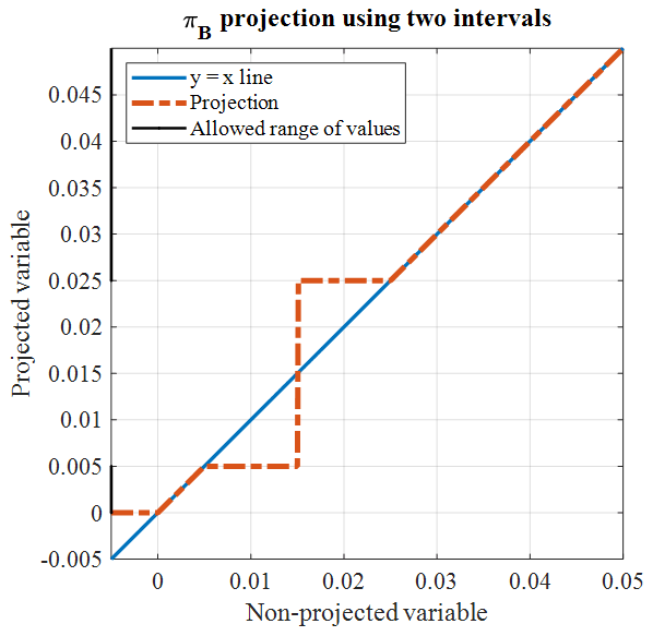
The modified version of the structural model of Pakyuz-Charrier (2018) used here is given in Giraud and Seillé (2022). It also contains the synthetic MT and magnetic data used. The field data can be obtained from the Geological Survey of Queensland.
The version of the Tomofast-x inversion code used here was made publicly available by Ogarko et al. (2021b); the latest version is freely available at https://github.com/TOMOFAST/Tomofast-x (last access: 15 November 2022). The code used to perform the MT inversions is available at https://bitbucket.csiro.au/scm/~sei029/bmt1dinv.git (last access: 15 November 2022).
JG and HS designed the study with input from the rest of the authors. JG and HS and generated the magnetic and MT synthetic data, respectively. JG performed the magnetic data inversions. JG redacted the manuscript with input from HS, who is the main contributor to MT-related aspects, and comments from the rest of the authors. HS performed the synthetic MT data modelling with support from GV. HS and GV derived the MT depth to basement results used in the case study. MDL and MWJ provided geological support and knowledge. MDL participated in both the geological and geophysical interpretation of the results and edited the relevant sections of the manuscript. MDL provided detailed comments during its redaction. GV participated in the design of the methodology and the interpretation of results. JG and HS prepared the datasets for public release.
VO and JG worked together on the development and testing of functionalities of Tomofast-x that are introduced and applied in the presented work. All authors provided feedback on the different versions of the manuscript and during the progress of the study.
The contact author has declared that none of the authors has any competing interests.
Publisher's note: Copernicus Publications remains neutral with regard to jurisdictional claims in published maps and institutional affiliations.
Jérémie Giraud, Mark D. Lindsay, and Mark W. Jessell were supported, in part, by Loop – 25 Enabling Stochastic 3D Geological Modelling (LP170100985) and the Mineral Exploration Cooperative Research Centre, whose activities are funded by the Australian Government's Cooperative Research Centre Program. This is MinEx CRC Document 2021/36. Mark D. Lindsay was supported by ARC DECRA DE190100431. Hoël Seillé and Gerhard Visser were supported by the CSIRO Deep Earth Imaging Future Science Platform. We acknowledge the developers of the ModEM code for making it available. Jérémie Giraud has received funding from the European Union's Horizon 2020 research and innovation programme under the Marie Skłodowska-Curie grant agreement no. 101032994.
This research has been supported by the Department of Industry, Science, Energy and Resources of the Australian Government (grant no. GA22270). Australia Research Council (grant DE190100431), and European Commission (grant no. 101032994).
This paper was edited by Charlotte Krawczyk and reviewed by Kristina Tietze and Max Moorkamp.
Agostinetti, N. P. and Bodin, T.: Flexible Coupling in Joint Inversions: A Bayesian Structure Decoupling Algorithm, J. Geophys. Res.-Sol. Ea., 123, 8798–8826, https://doi.org/10.1029/2018JB016079, 2018.
Anderson, C. G. and Logan, K. J.: The history and current status of geophysical exploration at the Osborne Cu & Au deposit, Mt. Isa, Explor. Geophys., 23, 1–7, https://doi.org/10.1071/EG992001, 1992.
Astic, T. and Oldenburg, D. W.: A framework for petrophysically and geologically guided geophysical inversion using a dynamic Gaussian mixture model prior, Geophys. J. Int., 219, 1989–2012, https://doi.org/10.1093/gji/ggz389, 2019.
Austin, J. and Blenkinsop, T.: The Cloncurry Lineament: Geophysical and geological evidence for a deep crustal structure in the Eastern Succession of the Mount Isa Inlier, Precambrian Res., 163, 50–68, https://doi.org/10.1016/j.precamres.2007.08.012, 2008.
Austin, J. R., Schmidt, P. W., and Foss, C. A.: Magnetic modeling of iron oxide copper-gold mineralization constrained by 3D multiscale integration of petrophysical and geochemical data: Cloncurry District, Australia, Interpretation, 1, T63–T84, https://doi.org/10.1190/INT-2013-0005.1, 2013.
Bhattacharyya, B. K.: Magnetic anomalies due to prism-shaped bodies with arbitrary polarization, GEOPHYSICS, 29, 517–531, 1964.
Bijani, R., Lelièvre, P. G., Ponte-Neto, C. F., and Farquharson, C. G.: Physical-property-, lithology- and surface-geometry-based joint inversion using Pareto Multi-Objective Global Optimization, Geophys. J. Int., 209, 730–748, https://doi.org/10.1093/gji/ggx046, 2017.
Blenkinsop, T.: Mount Isa inlier, Precambrian Res., 163, 1–6, https://doi.org/10.1016/j.precamres.2007.08.009, 2008.
Bodin, T. and Sambridge, M.: Seismic tomography with the reversible jump algorithm, Geophys. J. Int., 178, 1411–1436, https://doi.org/10.1111/j.1365-246X, 2009.
Boyd, S.: Distributed Optimization and Statistical Learning via the Alternating Direction Method of Multipliers, Foundations and Trends® in Machine Learning, 3, 1–122, https://doi.org/10.1561/2200000016, 2010.
Calcagno, P., Chilès, J. P., Courrioux, G., and Guillen, A.: Geological modelling from field data and geological knowledge. Part I. Modelling method coupling 3D potential-field interpolation and geological rules, Phys. Earth Planet. In., 171, 147–157, https://doi.org/10.1016/j.pepi.2008.06.013, 2008.
Caldwell, T. G., Bibby, H. M., and Brown, C.: The magnetotelluric phase tensor. Geophysical Journal International, 58, 457–469. https://doi.org/10.1111/j.1365-246X, 2004.
Case, G., Blenkinsop, T., Chang, Z., Huizenga, J. M., Lilly, R., and McLellan, J.: Delineating the structural controls on the genesis of iron oxide–Cu–Au deposits through implicit modelling: a case study from the E1 Group, Cloncurry District, Australia, Geol. Soc. London, Spec. Publ., 453, 349–384, https://doi.org/10.1144/SP453.4, 2018.
Chave, A. D., Jones, A. G., Mackie, R., and Rodi, W.: The Magnetotelluric Method, Cambridge University Press, Cambridge, https://doi.org/10.1017/CBO9781139020138, 2012.
Clark, D. A.: Magnetic effects of hydrothermal alteration in porphyry copper and iron-oxide copper–gold systems: A review, Tectonophysics, 624–625, 46–65, https://doi.org/10.1016/j.tecto.2013.12.011, 2014.
Conway, D., Simpson, J., Didana, Y., Rugari, J., and Heinson, G.: Probabilistic Magnetotelluric Inversion with Adaptive Regularisation Using the No-U-Turns Sampler, Pure Appl. Geophys., 175, 2881–2894, https://doi.org/10.1007/s00024-018-1870-5, 2018.
Èuma, M. and Zhdanov, M. S.: Massively parallel regularized 3D inversion of potential fields on CPUs and GPUs, Comput. Geosci., 62, 80–87, https://doi.org/10.1016/j.cageo.2013.10.004, 2014.
Èuma, M., Wilson, G. A., and Zhdanov, M. S.: Large-scale 3D inversion of potential field data, Geophys. Prospect., 60, 1186–1199, https://doi.org/10.1111/j.1365-2478.2011.01052.x, 2012.
Dentith, M. and Mudge, S. T.: Geophysics for the mineral exploration geologist, 438 pp., https://doi.org/10.1007/s00126-014-0557-9, 2014.
Dentith, M., Enkin, R. J., Morris, W., Adams, C., and Bourne, B.: Petrophysics and mineral exploration: a workflow for data analysis and a new interpretation framework, Geophys. Prospect., 68, 178–199, https://doi.org/10.1111/1365-2478.12882, 2020.
Dhnaram, C. and Greenwood, M.: 3D mineral potential of the Quamby area, 2013.
Egbert, G. D. and Kelbert, A.: Computational recipes for electromagnetic inverse problems, Geophys. J. Int., 189, 251–267, https://doi.org/10.1111/j.1365-246X.2011.05347.x, 2012.
Evans, R. L., Chave, A. D., Jones, A. G., Mackie, R., and Rodi, W.: Conductivity of Earth materials, in: The Magnetotelluric Method, Cambridge University Press, Cambridge, 50–95, https://doi.org/10.1017/CBO9781139020138.004, 2012.
Farquharson, C. G. and Oldenburg, D. W.: A comparison of automatic techniques for estimating the regularization parameter in non-linear inverse problems, Geophys. J. Int., 156, 411–425, https://doi.org/10.1111/j.1365-246X.2004.02190.x, 2004.
Gallardo, L. A. and Meju, M. A.: Characterization of heterogeneous near-surface materials by joint 2D inversion of dc resistivity and seismic data, Geophys. Res. Lett., 30, 1658, https://doi.org/10.1029/2003GL017370, 2003.
Gallardo, L. A., Fontes, S. L., Meju, M. A., Buonora, M. P., and de Lugao, P. P.: Robust geophysical integration through structure-coupled joint inversion and multispectral fusion of seismic reflection, magnetotelluric, magnetic, and gravity images: Example from Santos Basin, offshore Brazil, GEOPHYSICS, 77, B237–B251, https://doi.org/10.1190/geo2011-0394.1, 2012.
Giraud, J. and Seillé, H.: Datasets for the integration of MT data with magnetic inversion: proof-of-concept using synthetic data and field application, Zenodo [data set], https://doi.org/10.5281/zenodo.6340159, 2022.
Giraud, J., Pakyuz-Charrier, E., Jessell, M., Lindsay, M., Martin, R., and Ogarko, V.: Uncertainty reduction through geologically conditioned petrophysical constraints in joint inversion, GEOPHYSICS, 82, ID19–ID34, https://doi.org/10.1190/geo2016-0615.1, 2017.
Giraud, J., Lindsay, M., Ogarko, V., Jessell, M., Martin, R., and Pakyuz-Charrier, E.: Integration of geoscientific uncertainty into geophysical inversion by means of local gradient regularization, Solid Earth, 10, 193–210, https://doi.org/10.5194/se-10-193-2019, 2019a.
Giraud, J., Ogarko, V., Lindsay, M., Pakyuz-Charrier, E., Jessell, M., and Martin, R.: Sensitivity of constrained joint inversions to geological and petrophysical input data uncertainties with posterior geological analysis, Geophys. J. Int., 218, 666–688, https://doi.org/10.1093/gji/ggz152, 2019b.
Giraud, J., Lindsay, M., and Jessell, M.: Generalization of level-set inversion to an arbitrary number of geologic units in a regularized least-squares framework, GEOPHYSICS, 86, R623–R637, https://doi.org/10.1190/geo2020-0263.1, 2021a.
Giraud, J., Ogarko, V., Martin, R., Jessell, M., and Lindsay, M.: Structural, petrophysical, and geological constraints in potential field inversion using the Tomofast-x v1.0 open-source code, Geosci. Model Dev., 14, 6681–6709, https://doi.org/10.5194/gmd-14-6681-2021, 2021b.
Giraud, J., Seillé, H., Visser, G., Ogarko, V., Lindsay, M., and Jessell, M.: Utilisation of stochastic MT inversion results to constrain gravity inversion, in: 82nd EAGE Annual Conference & Exhibition, 1–5, https://doi.org/10.3997/2214-4609.202113105, 2021c.
Grose, L., Ailleres, L., Laurent, G., and Jessell, M.: LoopStructural 1.0: time-aware geological modelling, Geosci. Model Dev., 14, 3915–3937, https://doi.org/10.5194/gmd-14-3915-2021, 2021.
Guillen, A., Calcagno, P., Courrioux, G., Joly, A., and Ledru, P.: Geological modelling from field data and geological knowledge. Part II. Modelling validation using gravity and magnetic data inversion, Phys. Earth Planet. In., 171, 158–169, https://doi.org/10.1016/j.pepi.2008.06.014, 2008.
Haber, E. and Oldenburg, D.: Joint inversion: a structural approach, Inverse Probl., 13, 63–77, https://doi.org/10.1088/0266-5611/13/1/006, 1997.
Hansen, P. C. and Johnston, P. R.: The L-Curve and its Use in the Numerical Treatment of Inverse Problems, in: Computational Inverse Problems in Electrocardiography, edited by: Johnson, P., 119–142, 2001.
Heincke, B., Jegen, M., Moorkamp, M., Hobbs, R. W., and Chen, J.: An adaptive coupling strategy for joint inversions that use petrophysical information as constraints, J. Appl. Geophys., 136, 279–297, https://doi.org/10.1016/j.jappgeo.2016.10.028, 2017.
Jaccard, P.: Étude comparative de la distribution florale dans une portion des Alpes et du Jura, Bull. la Société Vaudoise des Sci. Nat., 37, 547–579, https://doi.org/10.5169/seals-266450, 1901.
Kelbert, A., Meqbel, N., Egbert, G. D., and Tandon, K.: ModEM: A modular system for inversion of electromagnetic geophysical data, Comput. Geosci., 66, 40–53, https://doi.org/10.1016/j.cageo.2014.01.010, 2014.
Lajaunie, C., Courrioux, G., and Manuel, L.: Foliation fields and 3D cartography .in geology: Principles of a method based on potential interpolation, Math. Geol., 29, 571–584, https://doi.org/10.1007/BF02775087, 1997.
Lampinen, H., Occhipinti, S., Lindsay, M., and Laukamp, C.: Magnetic susceptibility of Edmund Basin, Capricorn Orogen, WA, ASEG Ext. Abstr., 2016, 1–8, https://doi.org/10.1071/aseg2016ab254, 2016.
Le, C. V. A., Harris, B. D., Pethick, A. M., Takam Takougang, E. M., and Howe, B.: Semiautomatic and Automatic Cooperative Inversion of Seismic and Magnetotelluric Data, Surv. Geophys., 37, 845–896, https://doi.org/10.1007/s10712-016-9377-z, 2016.
Le Pape, F., Jones, A. G., Jessell, M. W., Perrouty, S., Gallardo, L. A., Baratoux, L., Hogg, C., Siebenaller, L., Touré, A., Ouiya, P., and Boren, G.: Crustal structure of southern Burkina Faso inferred from magnetotelluric, gravity and magnetic data, Precambrian Res., 300, 261–272, https://doi.org/10.1016/j.precamres.2017.08.013, 2017.
Lelièvre, P., Farquharson, C., and Hurich, C.: Joint inversion of seismic traveltimes and gravity data on unstructured grids with application to mineral exploration, GEOPHYSICS, 77, K1–K15, https://doi.org/10.1190/geo2011-0154.1, 2012.
Lelièvre, P. G. and Farquharson, C. G.: Integrated Imaging for Mineral Exploration, in: Integrated Imaging of the Earth: Theory and Applications, edited by: Moorkamp, M., Lelièvre, P. G., Linde, N. and Khan, A., 137–166, https://doi.org/10.1002/9781118929063.ch8, 2016.
Li, Y. and Oldenburg, D. W.: Fast inversion of large-scale magnetic data using wavelet transforms, Geophys. J. Int., 152, 251–265, https://doi.org/10.1046/j.1365-246X.2003.01766.x, 2003.
Lines, L. R., Schultz, A. K., and Treitel, S.: Cooperative inversion of geophysical data, GEOPHYSICS, 53, 8–20, https://doi.org/10.1190/1.1442403, 1988.
Malinverno, A.: Parsimonious Bayesian Markov chain Monte Carlo inversion in a nonlineargeophysical problem, Geophys. J. Int., 151, 675–688, https://doi.org/10.1046/j.1365-246X, 2002.
Manassero, M. C., Afonso, J. C., Zyserman, F., Zlotnik, S., and Fomin, I.: A reduced order approach for probabilistic inversions of 3-D magnetotelluric data I: general formulation, Geophys. J. Int., 223, 1837–1863, https://doi.org/10.1093/gji/ggaa415, 2020.
Martin, R., Monteiller, V., Komatitsch, D., Perrouty, S., Jessell, M., Bonvalot, S., and Lindsay, M. D.: Gravity inversion using wavelet-based compression on parallel hybrid CPU/GPU systems: application to southwest Ghana, Geophys. J. Int., 195, 1594–1619, https://doi.org/10.1093/gji/ggt334, 2013.
Martin, R., Giraud, J., Ogarko, V., Chevrot, S., Beller, S., Gégout, P., and Jessell, M.: Three-dimensional gravity anomaly inversion in the Pyrenees using compressional seismic velocity model as structural similarity constraints, Geophys. J. Int., 225, 1063–1085, https://doi.org/10.1093/gji/ggaa414, 2020.
Martin, R., Giraud, J., Ogarko, V., Chevrot, S., Beller, S., Gégout, P., and Jessell, M.: Three-dimensional gravity anomaly data inversion in the Pyrenees using compressional seismic velocity model as structural similarity constraints, Geophys. J. Int., 225, 1063–1085, https://doi.org/10.1093/gji/ggaa414, 2021.
Moorkamp, M.: Integrating Electromagnetic Data with Other Geophysical Observations for Enhanced Imaging of the Earth: A Tutorial and Review, Surv. Geophys., 1–28, https://doi.org/10.1007/s10712-017-9413-7, 2017.
Moorkamp, M.: Joint inversion of gravity and magnetotelluric data from the Ernest-Henry IOCG deposit with a variation of information constraint, in: First International Meeting for Applied Geoscience & Energy Expanded Abstracts, 1711–1715, https://doi.org/10.1190/segam2021-3582000.1, 2021.
Moorkamp, M., Heincke, B., Jegen, M., Hobbs, R. W., and Roberts, A. W.: Joint Inversion in Hydrocarbon Exploration, in: Integrated Imaging of the Earth: Theory and Applications, 167–189, https://doi.org/10.1002/9781118929063.ch9, 2016.
Ogarko, V., Giraud, J., Martin, R., and Jessell, M.: Disjoint interval bound constraints using the alternating direction method of multipliers for geologically constrained inversion: Application to gravity data, GEOPHYSICS, 86, G1–G11, https://doi.org/10.1190/geo2019-0633.1, 2021a.
Ogarko, V., Giraud, J., and Martin, R.: Tomofast-x v1.0 source code, Zenodo [code], https://doi.org/10.5281/zenodo.4454220, 2021b.
Oliver-Ocaño, F. M., Gallardo, L. A., Romo-Jones, J. M., and Pérez-Flores, M. A.: Structure of the Cerro Prieto Pull-apart basin from joint inversion of gravity, magnetic and magnetotelluric data, J. Appl. Geophys., 170, 103835, https://doi.org/10.1016/j.jappgeo.2019.103835, 2019.
Paige, C. C. and Saunders, M. A.: LSQR: An Algorithm for Sparse Linear Equations and Sparse Least Squares, ACM T. Math. Software, 8, 43–71, https://doi.org/10.1145/355984.355989, 1982.
Pakyuz-Charrier, E., Lindsay, M., Ogarko, V., Giraud, J., and Jessell, M.: Monte Carlo simulation for uncertainty estimation on structural data in implicit 3-D geological modeling, a guide for disturbance distribution selection and parameterization, Solid Earth, 9, 385–402, https://doi.org/10.5194/se-9-385-2018, 2018.
Pakyuz-Charrier, E., Jessell, M., Giraud, J., Lindsay, M., and Ogarko, V.: Topological analysis in Monte Carlo simulation for uncertainty propagation, Solid Earth, 10, 1663–1684, https://doi.org/10.5194/se-10-1663-2019, 2019.
Pakyuz-Charrier, E. I. G.: Mansfield (Victoria, Australia) area original GeoModeller model and relevant MCUE outputs, Zenodo [data set], https://doi.org/10.5281/zenodo.848225, 2018.
Peng, M., Tan, H., and Moorkamp, M.: Structure-Coupled 3-D Imaging of Magnetotelluric and Wide-Angle Seismic Reflection/Refraction Data With Interfaces, J. Geophys. Res.-Sol. Ea., 124, 10309–10330, https://doi.org/10.1029/2019JB018194, 2019.
Portniaguine, O. and Zhdanov, M. S.: 3-D magnetic inversion with data compression and image focusing, GEOPHYSICS, 67, 1532–1541, https://doi.org/10.1190/1.1512749, 2002.
Ren, Z. and Kalscheuer, T.: Uncertainty and Resolution Analysis of 2D and 3D Inversion Models Computed from Geophysical Electromagnetic Data, Surv. Geophys., 41, 47–112, https://doi.org/10.1007/s10712-019-09567-3, 2019.
Rodi, W. L., Mackie, R. L., Chave, A. D., Jones, A. G., Mackie, R., and Rodi, W.: The inverse problem, in: The Magnetotelluric Method, edited by: Chave, A. D. and Jones, A. G., Cambridge University Press, Cambridge, 347–420, https://doi.org/10.1017/CBO9781139020138.010, 2012.
Sambridge, M., Gallagher, K., Jackson, A., and Rickwood, P.: Trans-dimensional inverse problems,model comparison and the evidence, Geophys. J. Int., 167, 528–542, https://doi.org/10.1111/j.1365-246X, 2006.
Scalzo, R., Kohn, D., Olierook, H., Houseman, G., Chandra, R., Girolami, M., and Cripps, S.: Efficiency and robustness in Monte Carlo sampling for 3-D geophysical inversions with Obsidian v0.1.2: setting up for success, Geosci. Model Dev., 12, 2941–2960, https://doi.org/10.5194/gmd-12-2941-2019, 2019.
Schweizer, D., Blum, P., and Butscher, C.: Uncertainty assessment in 3-D geological models of increasing complexity, Solid Earth, 8, 515–530, https://doi.org/10.5194/se-8-515-2017, 2017.
Seillé, H. and Visser, G.: Bayesian inversion of magnetotelluric data considering dimensionality discrepancies, Geophys. J. Int., 223, 1565–1583, https://doi.org/10.1093/gji/ggaa391, 2020.
Seillé, H., Visser, G., Markov, J., and Simpson, J.: Probabilistic Cover-Basement Interface Map in Cloncurry, Australia, Using Magnetotelluric Soundings, J. Geophys. Res.-Sol. Ea., 126, e2021JB021883, https://doi.org/10.1029/2021JB021883, 2021.
Shannon, C. E. E.: A Mathematical Theory of Communication, Bell Syst. Tech. J., 27, 379–423, https://doi.org/10.1002/j.1538-7305.1948.tb01338.x, 1948.
Sun, J. and Li, Y.: Multidomain petrophysically constrained inversion and geology differentiation using guided fuzzy c-means clustering, Geophysics, 80, ID1–ID18, https://doi.org/10.1190/geo2014-0049.1, 2015.
Tarantola, A.: Inverse Problem Theory and Methods for Model Parameter Estimation, Society for Industrial and Applied Mathematics, Philadelphia, https://doi.org/10.1137/1.9780898717921, 2005.
Tikhonov, A. N. and Arsenin, V. Y.: Solution of Ill-Posed Problems, Math. Comput., 32, 491, https://doi.org/10.2307/2006360, 1978.
Tveit, S., Mannseth, T., Park, J., Sauvin, G., and Agersborg, R.: Combining CSEM or gravity inversion with seismic AVO inversion, with application to monitoring of large-scale CO2 injection, Comput. Geosci., 24, 1201–1220, https://doi.org/10.1007/s10596-020-09934-9, 2020.
Visser, G.: Smart stitching: adding lateral priors to ensemble inversions as a post-processing step, ASEG Ext. Abstr., 2019, 1–4, https://doi.org/10.1080/22020586.2019.12073075, 2019.
Visser, G. and Markov, J.: Cover thickness uncertainty mapping using Bayesian estimate fusion: leveraging domain knowledge, Geophys. J. Int., 219, 1474–1490, https://doi.org/10.1093/gji/ggz358, 2019.
Wellmann, F. and Caumon, G.: 3-D Structural geological models: Concepts, methods, and uncertainties, edited by: Schmelzback, C., Cambridge, Massachusetts, 1–121, https://doi.org/10.1016/bs.agph.2018.09.001, 2018.
Wellmann, J. F. and Regenauer-Lieb, K.: Uncertainties have a meaning: Information entropy as a quality measure for 3-D geological models, Tectonophysics, 526–529, 207–216, https://doi.org/10.1016/j.tecto.2011.05.001, 2012.
Xiang, E., Guo, R., Dosso, S. E., Liu, J., Dong, H., and Ren, Z.: Efficient hierarchical trans-dimensionalBayesian inversion of magnetotelluric data, Geophys. J. Int., 213, 1751–1767, 2018.
Zhang, R., Li, T., Deng, X., Huang, X., and Pak, Y.: Two-dimensional data-space joint inversion of magnetotelluric, gravity, magnetic and seismic data with cross-gradient constraints, Geophys. Prospect., 68, 721–731, https://doi.org/10.1111/1365-2478.12858, 2020.