Lahar events in the last 2000 years from Vesuvius eruptions – Part 2: Formulation and validation of a computational model based on a shallow layer approach

In this paper we present a new model for the simulation of lahars based on the depth-averaged code IMEX-SfloW2D with new governing and constitutive equations introduced to better describe the dynamics of lahars. A thorough sensitivity analysis is carried out to identify the critical processes (such as erosion and deposition) and parameters (both numerical and physical) controlling lahar runout using both synthetic and real case topographies. In particular, an application of the model to a syn-eruptive lahar from a reference size eruption from Somma–Vesuvius, affecting the Campanian Plain (southern Italy), described in Di Vito et al. (2024), is used in this work for the sensitivity analysis. Effects of erosion and deposition are investigated by comparing simulations with and without these processes. By comparing flow thickness and area covered by the flow and their evolution with time, we show that the modelling of both the processes is important to properly simulate the effects of the bulking and debulking as well as the associated changes in rheology. From a computational point of view, the comparisons of simulations obtained for different numerical grids (from 25 to 100 m), scheme order, and grain size discretization were useful to find a good compromise between resolution and computational speed. The companion paper by Sandri et al. (2024) shows an application of the presented model for probabilistic volcanic hazard assessment for lahars from Vesuvius deposits in the Neapolitan area.

1 Introduction

Water-saturated flows made from volcanic deposits are known as “lahars”, which is an Indonesian term used to indicate muddy flows. As typical in the volcanological literature, here we will use the term lahar to denote any water-saturated flows from hyperconcentrated flow carrying up to 50 vol % sediment to lower-concentration flows (< 10 % sediment). These wet granular flows are commonly characterized by a high flow density and can have high flow velocity, generating large dynamic pressures able to destroy even buildings and infrastructures. Moreover, this kind of flow can inundate large areas, disrupting ground transportation networks, human settlements, power lines, industry, and agriculture (e.g. Zanchetta et al., 2004).

Lahars can form from the remobilization of unconsolidated tephra, such as for the hundreds of lahars generated by torrential rains after the 1991 Pinatubo eruption in the Philippines (Van Westen and Daag, 2005). In other cases, such as at Mount St. Helens, lahars can result from dome collapses and the associated volcanic explosions (Scott, 1988). Additionally, devastating lahars can form when a pyroclastic flow melts snow or ice caps (Major and Newhall, 1989), such as for the 1995 eruption on the glaciated Nevado del Ruiz, Colombia (Pierson et al., 1990). Mt. Rainier is another example of a volcano that experienced several lahars of this kind in the past. Lahars can also form in eruptions beneath crater lakes, such as at Keluth, Indonesia (Mastin and Witter, 2000), and Ruapehu, New Zealand (Lecointre et al., 2004).

If lahars are generated before, during, or after the eruption they are named pre-eruptive, syn-eruptive, or post-eruptive lahars (Vallance and Iverson, 1995). The term syn-eruptive must not be taken literally but indicates a lahar generated during or in the period immediately following an eruption. Besides a triggering mechanism, generation of a lahar requires (i) an adequate water source, which can be hydrothermal water, rapidly melted snow and ice, crater lake water, and rainfall runoff; (ii) abundant unconsolidated debris that typically includes pyroclastic flow and fall deposits, glacial drift, colluvium, and soil; and (iii) steep slopes and substantial relief at the source (Aspinall et al., 2016). Because lahars are water-saturated flows, for which both liquid and solid interactions are fundamental, their behaviour is different from other related phenomena common to volcanoes such as debris avalanches and floods. In terms of fragment size distribution, the material carried by lahars ranges in diameter from about 10⁻⁶ to 10 m. Lahars can have temperature up to 100 °C and can change character downstream through processes of flow bulking (erosion and incorporation of secondary debris as they move downstream) and debulking (a process in which the lahar selectively deposits certain particles, owing to their size or density, as it moves downstream). Primary particles in lahar deposits derive from contemporaneous eruption deposits or, in the case of avalanche-induced lahar deposits, from the original avalanche mass; secondary particles derive from the erosion and incorporation of downstream volcaniclastic debris, alluvium, colluvium glacial drift, and bedrock. Many properties of lahars including, but not limited to, particle concentration, granulometry and componentry, bulk rheology, and velocity are highly variable in both time (i.e. unsteadiness) and space (i.e. non-uniformity).

Several methods have been proposed to assess the related hazard, ranging from simple empirical models like LAHARZ (Iverson et al., 1998), which can be used to estimate the inundated areas, to geophysical mass flow models which use different rheological laws, such as Newtonian, Bingham, Bagnold, or Coulomb models, depending on flow behaviour (e.g. TITAN2D, Pitman et al., 2003; Patra et al., 2005; FLO2D, O'Brien et al., 1993; VolcFlow, Kelfoun and Druitt, 2005; Kelfoun et al., 2009), and can furnish values of critical variables, such as velocity and dynamic pressure. A different approach, based on a fully three-dimensional model of two-phase flows, can be found in Dartevelle (2004) and Meruane et al. (2010). One of the most general two-phase debris-flow models was developed by Pudasaini (2012), and it includes many essential physical phenomena observable in debris flows. Mohr–Coulomb plasticity is used to close the solid stress. The reader is referred to Pudasaini (2012) and references therein for a general review of the topic. More recently, building on the Pudasaini (2012) two-phase flow model, Pudasaini and Margili (2019) presented a new mass flow model (r.avaflow, https://www.landslidemodels.org/r.avaflow, last access: 9 February 2024) accounting for the complexity of geomorphic mass flows consisting of coarse particles, fine particles, and viscous fluid.

In this work we present a new simplified model developed for lahar hazard assessment. The model, discussed in Sect. 2, is based on the Saint-Venant depth-averaged equations, coupled with source terms accounting for friction and with terms for erosion and deposition of solid particles. Then in Sect. 3 we present a few examples of model validation and applications and in Sect. 4 a short discussion and conclusion.

2 Physical–numerical model

The physical model for lahars is based on the shallow layer approach and on the solutions of a set of depth-averaged transport equations. As we explain below the numerical solution was obtained by modifying the IMEX-SfloW2D code (de' Michieli-Vitturi et al., 2019, 2023), with new governing and constitutive equations introduced to better simulate lahars dynamics. In this section, we briefly introduce all model variables, and we describe the governing equations.

2.1 Model governing equations

2.1.1 Depth-averaged transport equations

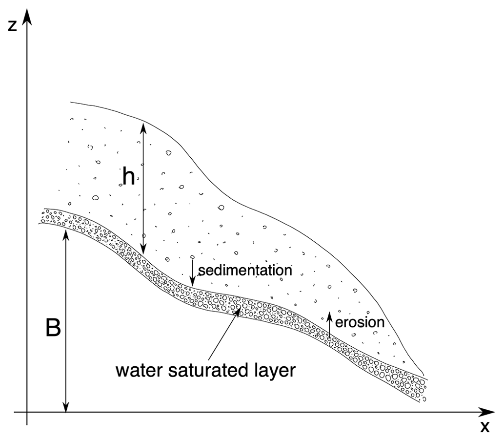
In this section, we present the set of partial differential equations governing the dynamics of lahars. Assuming that the lahar flow is a homogeneous mixture of water and n_s solid phases (see Fig. 1), its density ${\mathit{\rho }}_{\mathrm{m}}\left(x,y,t\right)$ is defined in terms of the volumetric fractions α_(⋅) and densities ρ_(⋅) of the components:

$$\begin{array}{}\text{(1)}& {\mathit{\rho }}_{\mathrm{m}}={\mathit{\alpha }}_{\mathrm{w}}{\mathit{\rho }}_{\mathrm{w}}+\sum _{i_{\mathrm{s}}=\mathrm{1}}^{n_{\mathrm{s}}}{\mathit{\alpha }}_{\mathrm{s},i_{\mathrm{s}}}{\mathit{\rho }}_{\mathrm{s},i_{\mathrm{s}}},\end{array}$$

where the subscript w denotes the water phase and the subscripts s denotes the class i_s of the solid phase. Equations are written in global Cartesian coordinates (x,y), with x and y orthogonal to the z axis, assumed to be parallel to gravitational acceleration $\mathit{g}=\left(\mathrm{0},\mathrm{0},g\right)$. We denote the flow thickness with $h\left(x,y,t\right)$ and the depth-averaged horizontal components of the flow velocity with $u\left(x,y,t\right)$ and $v\left(x,y,t\right)$, assuming that, due to the flow turbulence, solid phases are well-mixed with the liquid carrier phases and they have the same horizontal velocity. The flow moves over a topography, described by the variable $B\left(x,y,t\right)$. In principle, topography can change with time, but as a first approximation we neglect the changes associated with erosion and deposition, while these processes are modelled and accounted for the flow dynamics. Thus, we assume the topography to be a function of space only.

Figure 1 Sketch of the lahar.

With the notation introduced above, conservation of mass for the flow mixture is written in the following way:

$$\begin{array}{}\text{(2)}& \begin{array}{rl}& {\displaystyle \frac{\partial {\mathit{\rho }}_{\mathrm{m}}h}{\partial t}}+{\displaystyle \frac{\partial \left({\mathit{\rho }}_{\mathrm{m}}hu\right)}{\partial x}}+{\displaystyle \frac{\partial \left({\mathit{\rho }}_{\mathrm{m}}hv\right)}{\partial y}}\\ & =\sum _{i_{\mathrm{s}}=\mathrm{1}}^{n_{\mathrm{s}}}\left[{\mathit{\rho }}_{\mathrm{s},i_{\mathrm{s}}}\right(E_{\mathrm{s},i_{\mathrm{s}}}-D_{\mathrm{s},i_{\mathrm{s}}}\left)\right]\\ & +{\mathit{\rho }}_{\mathrm{w}}\left\{D_{\mathrm{w}}+{\displaystyle \frac{{\mathit{\alpha }}_{\mathrm{d}}}{\mathrm{1}-{\mathit{\alpha }}_{\mathrm{d}}}}\sum _{i_{\mathrm{s}}=\mathrm{1}}^{n_{\mathrm{s}}}\left[\right(E_{\mathrm{s},i_{\mathrm{s}}}-D_{\mathrm{s},i_{\mathrm{s}}}\left)\right]\right\},\end{array}\end{array}$$

where E_s and D_s are the volumetric rate of erosion and deposition of solid particles, respectively, and D_w is the rate of loss of water, not associated with the deposition of particles (for example, associated with evaporation or other processes). The first term on the right-hand side accounts for the loss and entrainment of solid particles, while the last term accounts for the loss of water. This term accounts not only for the loss due to the rate D_w, but also for the loss associated with particle erosion and sedimentation. In fact, we assume both the pre-existing erodible layer and the flow deposit to be water-saturated, with the volume fraction of water given by α_w.

The two equations for momentum conservation are

$$\begin{array}{}\text{(3a)}& {\displaystyle }\begin{array}{rl}& {\displaystyle \frac{\partial \left({\mathit{\rho }}_{\mathrm{m}}hu\right)}{\partial t}}+{\displaystyle \frac{\partial }{\partial x}}\left({\mathit{\rho }}_{\mathrm{m}}h{u}^{\mathrm{2}}+{\displaystyle \frac{\mathrm{1}}{\mathrm{2}}}{\mathit{\rho }}_{\mathrm{m}}g{h}^{\mathrm{2}}\right)+{\displaystyle \frac{\partial }{\partial y}}\left({\mathit{\rho }}_{\mathrm{m}}huv\right)\\ & =-{\mathit{\rho }}_{\mathrm{m}}gh{\displaystyle \frac{\partial B}{\partial x}}+F_x\\ & -u\left[\sum _{i_{\mathrm{s}}=\mathrm{1}}^{n_{\mathrm{s}}}\left({\mathit{\rho }}_{\mathrm{s},i_{\mathrm{s}}}{D}_{\mathrm{s},i_{\mathrm{s}}}\right)+{\mathit{\rho }}_{\mathrm{w}}\left(D_{\mathrm{w}}+{\displaystyle \frac{{\mathit{\alpha }}_{\mathrm{d}}}{\mathrm{1}-{\mathit{\alpha }}_{\mathrm{d}}}}\sum _{i_{\mathrm{s}}=\mathrm{1}}^{n_{\mathrm{s}}}{D}_{\mathrm{s},i_{\mathrm{s}}}\right)\right],\end{array}\text{(3b)}& {\displaystyle }\begin{array}{rl}& {\displaystyle \frac{\partial \left({\mathit{\rho }}_{\mathrm{m}}hv\right)}{\partial t}}+{\displaystyle \frac{\partial }{\partial x}}\left({\mathit{\rho }}_{\mathrm{m}}huv\right)+{\displaystyle \frac{\partial }{\partial y}}\left({\mathit{\rho }}_{\mathrm{m}}h{v}^{\mathrm{2}}+{\displaystyle \frac{\mathrm{1}}{\mathrm{2}}}{\mathit{\rho }}_{\mathrm{m}}g{h}^{\mathrm{2}}\right)=\\ & -{\mathit{\rho }}_{\mathrm{m}}gh{\displaystyle \frac{\partial B}{\partial y}}+F_{\mathrm{y}}\\ & -v\left[\sum _{i_{\mathrm{s}}=\mathrm{1}}^{n_{\mathrm{s}}}\left({\mathit{\rho }}_{\mathrm{s},i_{\mathrm{s}}}{D}_{\mathrm{s},i_{\mathrm{s}}}\right)+{\mathit{\rho }}_{\mathrm{w}}\left(D_{\mathrm{w}}+{\displaystyle \frac{{\mathit{\alpha }}_{\mathrm{d}}}{\mathrm{1}-{\mathit{\alpha }}_{\mathrm{d}}}}\sum _{i_{\mathrm{s}}=\mathrm{1}}^{n_{\mathrm{s}}}{D}_{\mathrm{s},i_{\mathrm{s}}}\right)\right],\end{array}\end{array}$$

where $\mathit{F}=\left(F_x,F_{\mathrm{y}}\right)$ is the vector of frictional forces and the last term on the right-hand side of both the equations considers the loss of momentum associated with particle sedimentation. Please note that there are no terms associated with erosion of solid particles in the momentum equations because they do not carry any horizontal momentum within the flow, although they change the inertia terms.

Flow temperature T changes with entrainment of water and solid particles eroded from the underlying terrain, and this in turn can change lahar properties (for example, viscosity). For this reason, we also solve for a transport equation for the internal energy e=C_vT (with C_v being the mass-averaged specific heat in the flow):

$$\begin{array}{}\text{(4)}& \begin{array}{rl}& {\displaystyle \frac{\partial }{\partial t}}\left({\mathit{\rho }}_{\mathrm{m}}he\right)+{\displaystyle \frac{\partial }{\partial x}}\left({\mathit{\rho }}_{\mathrm{m}}hue\right)+{\displaystyle \frac{\partial }{\partial y}}\left({\mathit{\rho }}_{\mathrm{m}}hve\right)\\ & =\sum _{i_{\mathrm{s}}=\mathrm{1}}^{n_{\mathrm{s}}}\left[{\mathit{\rho }}_{\mathrm{s},i_{\mathrm{s}}}{C}_{\mathrm{s},i_{\mathrm{s}}}\left(T_{\mathrm{s}}{E}_{\mathrm{s},i_{\mathrm{s}}}-T{D}_{\mathrm{s},i_{\mathrm{s}}}\right)\right]\\ & +{\mathit{\rho }}_{\mathrm{w}}{C}_{\mathrm{w}}{\displaystyle \frac{{\mathit{\alpha }}_{\mathrm{d}}}{\mathrm{1}-{\mathit{\alpha }}_{\mathrm{d}}}}\sum _{i_{\mathrm{s}}=\mathrm{1}}^{n_{\mathrm{s}}}\left[\left(T_{\mathrm{s}}{E}_{\mathrm{s},i_{\mathrm{s}}}-T{D}_{\mathrm{s},i_{\mathrm{s}}}\right)\right],\end{array}\end{array}$$

where C_s and C_w are the specific heats of solid and water, respectively, and T_s is the substrate temperature before erosion. In this equation, heat transfer by thermal conduction is neglected, as are thermal radiation and heating due to friction.

Additional transport equations for the mass of n_s solid classes are also considered.

$$\begin{array}{}\text{(5)}& \begin{array}{rl}& \partial {\displaystyle \frac{\left({\mathit{\alpha }}_{\mathrm{s},i_{\mathrm{s}}}{\mathit{\rho }}_{\mathrm{s},i_{\mathrm{s}}}h\right)}{\partial t}}+{\displaystyle \frac{\partial \left({\mathit{\alpha }}_{\mathrm{s},i_{\mathrm{s}}}{\mathit{\rho }}_{\mathrm{s},i_{\mathrm{s}}}hu\right)}{\partial x}}+{\displaystyle \frac{\partial \left({\mathit{\alpha }}_{\mathrm{s},i_{\mathrm{s}}}{\mathit{\rho }}_{\mathrm{s},i_{\mathrm{s}}}hv\right)}{\partial y}}\\ & ={\mathit{\rho }}_{\mathrm{s},i_{\mathrm{s}}}\left(E_{\mathrm{s},i_{\mathrm{s}}}-D_{\mathrm{s},i_{\mathrm{s}}}\right)i_{\mathrm{s}}=\mathrm{1},\mathrm{\dots },n_{\mathrm{s}}\end{array}\end{array}$$

Finally, we have n_s equations for the volume of solid particles in the water-saturated erodible layer:

$$\begin{array}{}\text{(6)}& {\displaystyle \frac{\partial {\mathit{\alpha }}_{\mathrm{s},i_{\mathrm{s}}}{h}_{\mathrm{s},i_{\mathrm{s}}}}{\partial t}}=\left(E_{\mathrm{s},i_{\mathrm{s}}}-D_{\mathrm{s},i_{\mathrm{s}}}\right)i_{\mathrm{s}}=\mathrm{1},\mathrm{\dots },n_{\mathrm{s}},\end{array}$$

where $h_{\mathrm{s},i_{\mathrm{s}}}$ is the thickness of each solid class in the layer, related to the total thickness h_e of this layer by the relationship

$$\begin{array}{}\text{(7)}& h_e={\displaystyle \frac{\mathrm{1}}{\mathrm{1}-{\mathit{\alpha }}_{\mathrm{w}}}}\sum _{i_{\mathrm{s}}=\mathrm{1}}^{n_{\mathrm{s}}}{h}_{\mathrm{s},i_{\mathrm{s}}}.\end{array}$$

2.1.2 Constitutive equations

The set of Eqs. (1)–(7) constitute a set of 4 + n_s partial differential equations for the unknown state variables Q=h, u, v, T, ${\mathit{\alpha }}_{\mathrm{s},\mathrm{1}},\mathrm{\dots },{\mathit{\alpha }}_{\mathrm{s},n_{\mathrm{s}}}$. In order to close the system and to be able to solve the equations, the terms accounting for friction, deposition, and erosion should be defined as functions of the state variables Q.

The friction term appearing in the momentum equations is written in the following way:

$$\begin{array}{}\text{(8)}& \mathit{F}=\left(F_x,F_{\mathrm{y}}\right)={\mathit{\rho }}_{\mathrm{m}}gh\left({\displaystyle \frac{u}{\sqrt{u^{\mathrm{2}}+v^{\mathrm{2}}}}}{s}_{\mathrm{f}},{\displaystyle \frac{u}{\sqrt{u^{\mathrm{2}}+v^{\mathrm{2}}}}}{s}_{\mathrm{f}}\right),\end{array}$$

where s_f is defined, according to O'Brien et al. (1993), as the total friction slope, given by the sum of three non-dimensional terms:

$$\begin{array}{}\text{(9)}& s_{\mathrm{f}}=s_{\mathrm{y}}+s_{\mathrm{v}}+s_{\mathrm{t}}.\end{array}$$

Here, s_y is the velocity-independent yield slope, s_v is the viscous slope, and s_t is the turbulent slope. These three terms, as done in the numerical code FLO-2D, are written in the following way:

$$\begin{array}{}\text{(10)}& s_{\mathrm{f}}={\displaystyle \frac{{\mathit{\tau }}_{\mathrm{y}}}{{\mathit{\rho }}_{\mathrm{m}}gh}}+{\displaystyle \frac{K\mathit{\mu }\sqrt{u^{\mathrm{2}}+v^{\mathrm{2}}}}{\mathrm{8}{\mathit{\rho }}_{\mathrm{m}}g{h}^{\mathrm{2}}}}+{\displaystyle \frac{n_{\mathrm{td}}^{\mathrm{2}}\left(u^{\mathrm{2}}+v^{\mathrm{2}}\right)}{h^{\mathrm{4}/\mathrm{3}}}},\end{array}$$

where τ_y is yield strength, K is an empirical resistance parameter, μ is fluid viscosity, and n_t is the Manning roughness coefficient. In the FLO-2D model (O'Brien et al., 1993), yield strength τ_y and fluid viscosity μ_m are defined through two empirical relationships derived from field observations:

$$\begin{array}{}\text{(11a)}& {\displaystyle }{\mathit{\mu }}_{\mathrm{m}}=a_{\mathrm{1}}\exp \left(b_{\mathrm{1}}{\mathit{\alpha }}_{\mathrm{s}}\right),\text{(11b)}& {\displaystyle }{\mathit{\tau }}_{\mathrm{y}}=a_{\mathrm{2}}\exp \left(b_{\mathrm{2}}{\mathit{\alpha }}_{\mathrm{s}}\right),\end{array}$$

where a_i and b_i are coefficients defined by laboratory experiments and α_s is the total volumetric fraction of solid (${\mathit{\alpha }}_{\mathrm{s}}={\sum }_{i_{\mathrm{s}}=\mathrm{1}}^{n_{\mathrm{s}}}{\mathit{\alpha }}_{\mathrm{s},i_{\mathrm{s}}})$. In the original formulation of O'Brien et al. (1993) the empirical parameters a₁ and b₁ are model constants, which do not vary with flow temperature. Here, we notice that the parameter a₁ has the units of a dynamic viscosity and it can be seen as the limit viscosity of the mixture when the dispersed solid fraction goes to zero. Thus, it should represent the dynamic viscosity of water. Commonly this parameter can be assumed to be constant, but in order to account for the dependence of water viscosity on its temperature, which could potentially affect lahar dynamics and runout, here we account for an additional correction factor Γ(T^c), which is a function of the temperature expressed in degrees Celsius:

$$\begin{array}{}\text{(12)}& a_{\mathrm{1}}=\left[{\mathit{\mu }}^{\mathrm{ref}}\cdot \mathrm{\Gamma }\left(T^{\mathrm{c}}\right)\right],\end{array}$$

where μ^ref denotes the viscosity at a reference temperature T^ref. Following Crittenden et al. (2012), the equation used to compute the factor Γ(T^c) is given by

$$\mathrm{\Gamma }\left(T\right)=C\cdot \mathit{\gamma }\cdot {\mathrm{10}}^A,$$

where the coefficients γ and A are given by

$$\begin{array}{c}{\displaystyle }\left\{\begin{array}{ll}\mathit{\gamma }={\mathrm{10}}^{-\mathrm{3}},& \mathrm{for}\mathrm{0}<T^{\mathrm{c}}<\mathrm{20}\mathit{°}\mathrm{C}\\ & \\ \mathit{\gamma }=\left(\mathrm{1.002}\cdot {\mathrm{10}}^{-\mathrm{3}}\right)\left({\mathrm{10}}^B\right),& \mathrm{for}{T}^{\mathrm{c}}\ge \mathrm{20}\mathit{°}\mathrm{C}\end{array}\right.\\ {\displaystyle }\left\{\begin{array}{ll}A=\frac{\mathrm{1301}}{\mathrm{998.333}+\mathrm{8.1855}\left(T^{\mathrm{c}}-\mathrm{20}\right)+\mathrm{0.00585}{\left(T^{\mathrm{c}}-\mathrm{20}\right)}^{\mathrm{2}}}-\mathrm{1.30223}& \mathrm{for}\mathrm{0}<T^{\mathrm{c}}<\mathrm{20}\mathit{°}\mathrm{C}\\ & \\ A=\frac{\mathrm{1.3272}\left(\mathrm{20}-T^{\mathrm{c}}\right)-\mathrm{0.001053}{\left(T^{\mathrm{c}}-\mathrm{20}\right)}^{\mathrm{2}}}{T^{\mathrm{c}}+\mathrm{105}}& \mathrm{for}{T}^{\mathrm{c}}\ge \mathrm{20}\mathit{°}\mathrm{C}\end{array}\right.\end{array}$$

and C is a constant such that $\mathrm{\Gamma }\left(T^{\mathrm{c},\mathrm{ref}}\right)=\mathrm{1}$. With this choice, when $T^{\mathrm{c}}=T^{\mathrm{c},\mathrm{ref}}$ and α_s=0, μ=μ^ref. With respect to the original work of O'Brian et al. (1993), the original relationship for yield strength has also been modified. In fact, here we take

$$\begin{array}{}\text{(13)}& {\mathit{\tau }}_{\mathrm{y}}=a_{\mathrm{2}}\left(\exp \left(b_{\mathrm{2}}{\mathit{\alpha }}_{\mathrm{s}}\right)-\mathrm{1}\right)\end{array}$$

In this way, yield stress disappears when solid fraction α_s goes to zero, recovering the Newtonian behaviour of water.

The values of the three components of the total friction slope (see Eq. 10) strongly depend on volumetric solid fraction, flow thickness, and velocity. In Fig. 2, for fixed values of the empirical parameters a_i and b_i (i= 1, 2) and for three different values of the total solid volume fraction (α_s=0.1 in Fig. 2a; α_s=0.35 in Fig. 2b; α_s=0.6 in Fig. 2c), we plotted the values of the three terms as a function of flow thickness and velocity. These diagrams (in logarithmic scale for all the variables) highlight how these terms can vary in a non-linear way by several orders of magnitude when thickness, velocity, and solid fraction vary in ranges that can be observed in lahars, potentially resulting in the presence of a stiff term in the system of equations. For this reason, a robust solver that allows the coupling between the gravitational and frictional terms is needed.

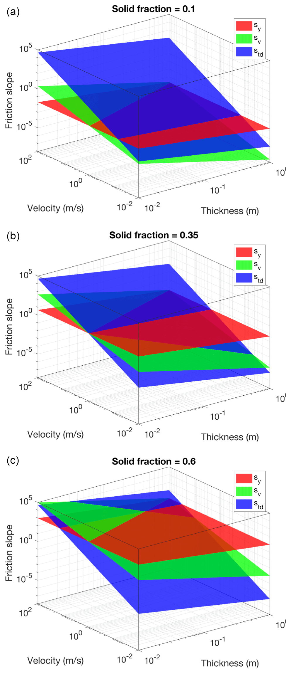
Figure 2 Contribution of the yield slope (s_y), viscous slope (s_v), and turbulent slope (s_td) to the total friction slope for three different solid volume fractions: 10 % (a), 35 % (b), and 60 % (c). The friction parameters have the following values: K=24.0, $a_{\mathrm{1}}=\mathrm{8.9}\cdot {\mathrm{10}}^{-\mathrm{4}}$, b₁=22.1, n_t=0.1, a₂=0.272, and $b_{\mathrm{2}}=\mathrm{22.0}.$

We also note that the presence of the yield strength term, i.e. a term independent of the velocity that opposes the motion, allows the flow to stop with a thickness that depends on the slope of the topography and on the fraction of solid material in the flow. This critical thickness can be calculated analytically and allows for the validation of the correct implementation of the discretization of the friction terms in the numerical model. Below we present a figure illustrating this relationship, where each line represents the critical thickness threshold line between the steady and unsteady condition for different total solid percentages in the flow. We can see that an increase of 10 % in the solid volume fraction for a fixed slope approximately corresponds to a factor of 4.5 increase in the critical thickness. We also observe that such a critical thickness is not only relevant for flow stoppage, but also for the initial triggering of the flow, and that this relationship can also be formulated in terms of critical liquid volume fraction. Thus, given a thickness of the permeable layer and a slope, we can compute the critical liquid volume fraction over which the lahar is triggered because the gravitational force exceeds the yield strength. For example, for a slope of 20° and a thickness of 1 m, a 60 % liquid volume would trigger a lahar, while a 50 % liquid volume would not. It is also worth noting that these critical thresholds depend on the values of the parameters for the yield strength.

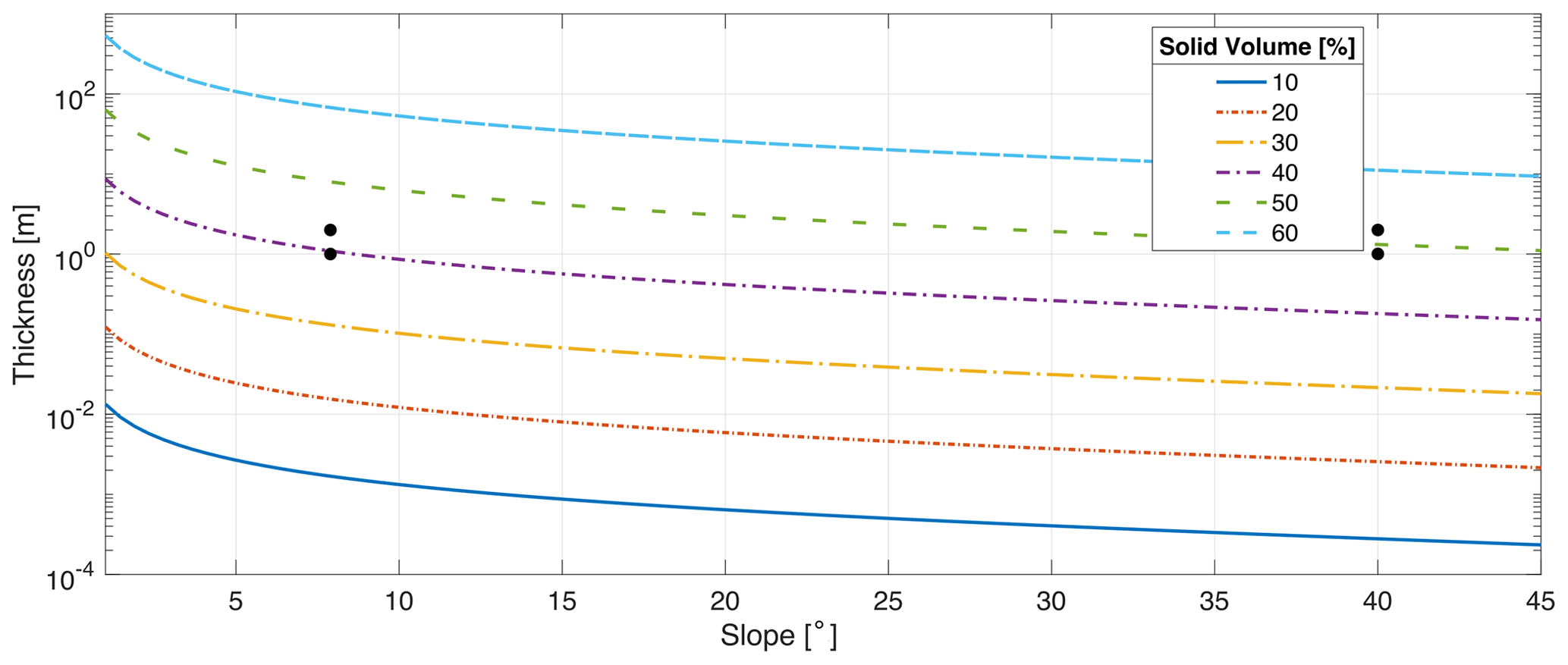
Figure 3 Critical thickness as a function of topography slope and solid volume fraction computed with the following values for the yield strength parameters: a₂=0.272 and $b_{\mathrm{2}}=\mathrm{22.0}.$ The four black dots represent couples of slope and thickness values used to test the capability of the numerical solver to properly reproduce the triggering conditions of lahars.

2.1.3 Erosion term

Following the parameterization by Fagents and Baloga (2006), we adopted an empirical relationship for the volumetric erosion rate E_tot of the substrate.

$$\begin{array}{}\text{(14)}& E_{\mathrm{tot}}=\mathit{ϵ}h\sqrt{u^{\mathrm{2}}+v^{\mathrm{2}}}\left(\mathrm{1}-{\mathit{\alpha }}_{\mathrm{s}}\right)\end{array}$$

This relation states that erosion is proportional to the thickness of the flow, the modulus of flow velocity, and the volumetric fraction of water in the flow through an empirical constant ϵ (with units [L]⁻¹). In the original work by Fagents and Baloga (2006), it is assumed that the rate of turbulent entrainment diminishes with increasing flow density. In fact, as the flow entrains solid sediment, turbulence is progressively dampened (Costa, 1988). Here, because the density is linearly proportional to the water volume fraction, we directly introduced a dependence of the erosion rate on this variable. From the total erosion rate, we compute the entrainment rates of the solid phases, which are then used in the governing equations, as

$$\begin{array}{}\text{(15)}& E_{i_{\mathrm{s}}}={\mathit{\beta }}_{i_{\mathrm{s}}}\left(\mathrm{1}-{\mathit{\alpha }}_{\mathrm{d}}\right)E_{\mathrm{tot}},\end{array}$$

where ${\mathit{\beta }}_{i_{\mathrm{s}}}$ represents the relative volumetric fractions of the solid particles in the erodible substrate ($\sum {\mathit{\beta }}_{i_{\mathrm{s}}}=\mathrm{1}$). When erosion occurs, not only solid particles are entrained in the flow, but also the water present in the deposit, here assumed to saturate its voids. This water entrainment from the erodible substrate is given by

$$\begin{array}{}\text{(16)}& E_{\mathrm{w}}={\mathit{\alpha }}_{\mathrm{d}}{E}_{\mathrm{tot}}.\end{array}$$

2.1.4 Sedimentation term

Sedimentation of particles from the flow is modelled as a volumetric flux at the flow bottom and is assumed to occur at a rate which is proportional to the volumetric fraction of particles in the flow and to the particle settling velocity $w_{\mathrm{s},i_{\mathrm{s}}}$:

$$\begin{array}{}\text{(17)}& D_{\mathrm{s},i_{\mathrm{s}}}={\mathit{\alpha }}_{\mathrm{s},i_{\mathrm{s}}}\cdot w_{\mathrm{s},i_{\mathrm{s}}}\left(d_{\mathrm{s},i_{\mathrm{s}}},{\mathit{\rho }}_{\mathrm{s},i_{\mathrm{s}}},{\mathit{\nu }}_{\mathrm{m}}\right).\end{array}$$

The particle settling velocity $w_{\mathrm{s},i_{\mathrm{s}}}$ is a function of the particle diameter $d_{\mathrm{s},i_{\mathrm{s}}}$, the particle density ${\mathit{\rho }}_{\mathrm{s},i_{\mathrm{s}}}$, and the mixture kinematic viscosity ${\mathit{\nu }}_{\mathrm{m}}=\frac{{\mathit{\mu }}_{\mathrm{m}}}{{\mathit{\rho }}_{\mathrm{m}}}$, and it is obtained by solving the following non-linear equation:

$$w_{\mathrm{s}}^{\mathrm{2}}\left(d_{\mathrm{s},i_{\mathrm{s}}}\right)C_{\mathrm{D}}\left(Re\right)={\displaystyle \frac{\mathrm{4}}{\mathrm{3}}}{d}_{\mathrm{s},i_{\mathrm{s}}}g\left({\displaystyle \frac{{\mathit{\rho }}_{\mathrm{s},i_{\mathrm{s}}}-{\mathit{\rho }}_{\mathrm{a}}}{{\mathit{\rho }}_{\mathrm{a}}}}\right).$$

The gas–particle drag coefficient C_D is a function of the particle Reynolds number ($Re=\frac{d_{\mathrm{s},i_{\mathrm{s}}}{w}_{\mathrm{s}}}{{\mathit{\nu }}_{\mathrm{m}}}$), and it is calculated by assuming spherical particles (although in the future it can be generalized for more realistic shapes; Bagheri et al., 2015; Dioguardi and Mele, 2015) through the following relations (Gidaspow, 1994):

$$\left\{\begin{array}{lcl}{C}_{\mathrm{D}}=\frac{\mathrm{24}}{Re}\left(\mathrm{1}+\mathrm{0.15}R{e}^{\mathrm{0.687}}\right)& & Re\le \mathrm{1000},\\ & & \\ C_{\mathrm{D}}=\mathrm{0.44}& & Re>\mathrm{1000}.\end{array}\right.$$

The dependence of the Reynolds number on the mixture kinematic viscosity acts on the settling velocity as a sort of hindered settling. In fact, mixture viscosity increases with the total volumetric fraction of solids, and thus the settling velocity decreases. This approach is described in Koo (2002), where several effective-medium models are analysed for determining settling velocities of particles in a viscous fluid. Effective-medium theories have been developed for predicting the transport properties of suspensions consisting of multiple particles in a fluid. In particular, the sedimentation velocity is computed using the effective viscosity of the suspension instead of the viscosity of the continuous phase.

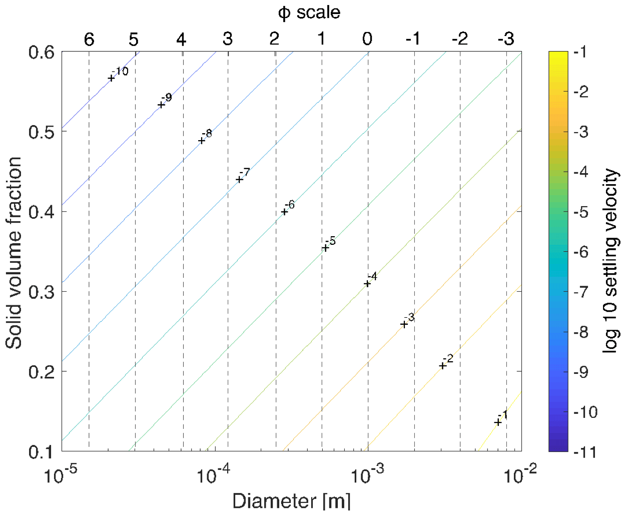
Figure 4 Effective settling velocity. Values of the settling velocity are represented by the different contours, as a function of particle diameter and total solid volume fraction.

When considering the settling of solid particles, it is important to remember that we assume the flow deposit formed because of sedimentation being saturated in water, with the volume fraction of water given by α_w. Thus, the lahar does not lose solid particles only because of sedimentation, but water too, with the volumetric deposition rate of water related to that of solid particles by the following equation:

$$\begin{array}{}\text{(18)}& D_{\mathrm{w}}={\displaystyle \frac{{\mathit{\alpha }}_{\mathrm{d}}}{\mathrm{1}-{\mathit{\alpha }}_{\mathrm{d}}}}\sum _{i_{\mathrm{s}}=\mathrm{1}}^{n_{\mathrm{s}}}{D}_{\mathrm{s},i_{\mathrm{s}}}.\end{array}$$

2.2 Numerical implementation

The numerical solution of the equations is based on the algorithm developed by de' Michieli Vitturi et al. (2019, 2023) for the code IMEX-SfloW2D, in particular on an operator splitting technique, where the advective, gravitational, and friction terms governing the fluid dynamics of the lahar are integrated in one step, while the erosion and deposition terms are integrated in a second step. This allows ad hoc numerical methods to be used for the different physical processes, optimizing and simplifying the overall solution process.

The numerical integration of the advective, gravitational, and friction terms is based on an implicit–explicit (IMEX) Runge–Kutta scheme, where the conservative fluxes and the gravitational terms are treated explicitly, while the stiff terms of the equations, represented by friction, are integrated implicitly. For the explicit spatial discretization of the fluxes, a modified version of the finite-volume central-upwind Kurganov and Petrova (2007) scheme has been adopted. The scheme, described in de' Michieli Vitturi et al. (2019, 2023) and Biagioli et al. (2021), has a second-order accuracy in space and guarantees the positivity of the flow thickness. The spatial accuracy is obtained with a discontinuous piecewise bilinear reconstruction of the flow variables in order to compute their values at the sides of each cell interface and thus the numerical fluxes. The slopes of the linear reconstructions of flow variables in the x and y direction are constrained by appropriate geometric limiters, allowing switching between low- and high-resolution schemes.

The implicit part of the IMEX Runge–Kutta scheme is solved using a Newton–Raphson method with an optimum step size control, where the Jacobian of the implicit terms is computed with a complex-step derivative approximation. The use of an implicit discretization of the stiff friction terms allows for larger time steps, controlled by the CFL condition, establishing a relationship between time step, flow velocity, and cell sizes.

After each Runge–Kutta procedure, the erosion, deposition, and air entrainment terms are integrated explicitly, and the flow variables and the topography at the centres of the computational cells are updated.

The numerical scheme is also designed to be well-balanced, i.e. to correctly preserve steady states. This property is important for the numerical simulation of lahars, for which the flow should be triggered only when the gravitational force exceeds the frictional forces, and thus a proper balance of these terms must also exist in the discretized equations resulting from the numerical schemes.

3 Model validation and applications

In this section we present a few applications of the proposed lahar model aimed at showing its robustness, applicability, and performance. Concerning the numerical tests aimed at demonstrating the mathematical accuracy for the code verification, the reader is referred to de' Michieli Vitturi et al. (2019, 2023) where the code IMEX-SfloW2D, on which our model is based, is presented. Applications of the code to hazard assessment for lahars in the Neapolitan area will be presented in the companion paper by Sandri et al. (2024).

Firstly, we present the case of a lahar flow on a synthetic topography in order to investigate the triggering conditions. Secondly, we introduce and describe all the needed variables to perform an application on real topography, which is the Valle di Avella, one of the Apennine valleys adjacent to Mt. Vesuvius, where in the companion papers by Di Vito et al. (2024) and Sandri et al. (2024) we also perform geological investigations and hazard analysis for lahars. In such a test area we explore the effects that can potentially affect the results, such as computational grid size, numerical scheme order, water temperature, discretization of the grain size distribution, and erosion and deposition terms. As the two latter processes are by far the most relevant for the key output variables such as run distance, flow thickness, and speed, in the last subsection we use field observations to calibrate erosion and deposition terms.

3.1 Simulations on a synthetic topography: lahar trigger conditions

The first set of simulations we present is aimed at testing the capability of the numerical code to properly reproduce the triggering conditions of a lahar in terms of the relationship between initial thickness, solid fraction, and slope. As previously stated, the values of the friction parameters controlling the yield strength define a unique relationship between thickness, slope, and solid fraction, resulting in a threshold for the mobility of the flow (see Fig. 2).

For the tests we consider a high- and low-angle slope (5 and 40°, respectively) and two values of the initial thickness (1 and 2 m) with different values of the solid fraction (30 % and 40 %).

The topography has a constant slope for x<0 m and is flat for x>0 m. In the left region of the domain, from x= −55 m to x= −50 m, the topography is excavated with a constant depth (1 or 2 m). Then, from x= −50 m, this region is connected to the original topography with a quadratic function in order to have a smooth transition and a horizontal slope at the right end. The excavated volume is then filled with the liquid–solid mixture. In this way the free-surface elevation of the initial volume corresponds to the original topography elevation. The topography and the free surface are shown in the panels of Fig. 5 with cyan and orange solid lines, respectively.

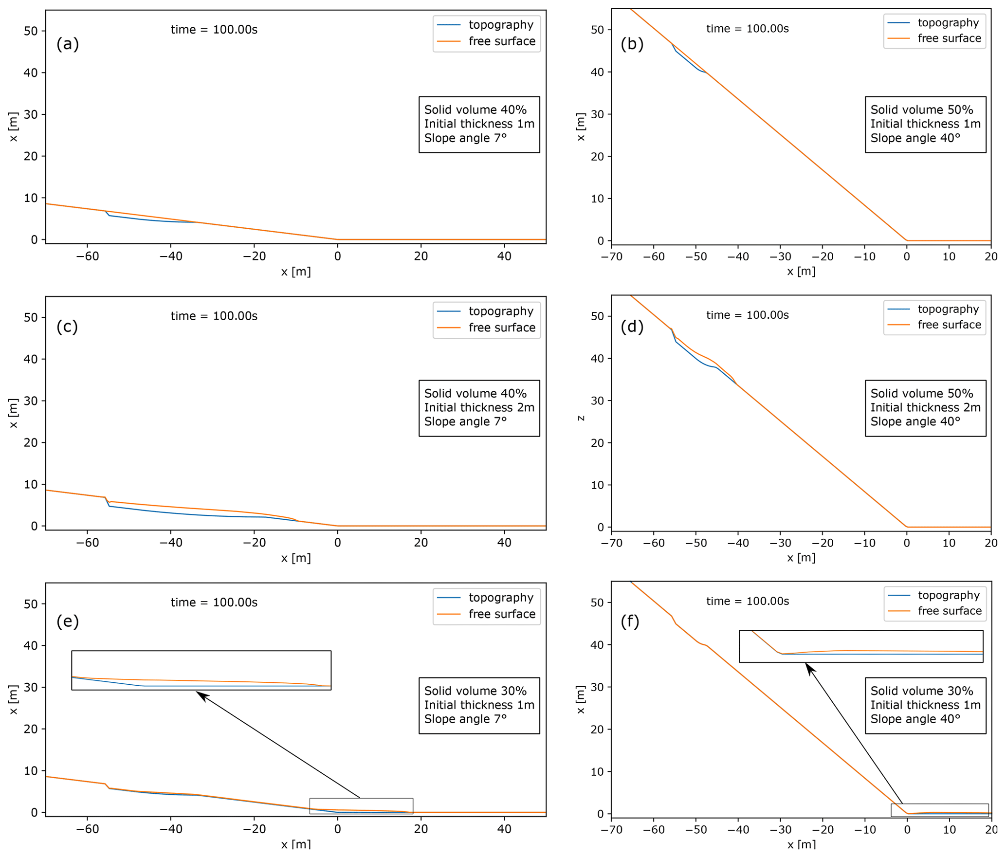
Figure 5 Flow free surface (red line) and topography (blue line) for six simulations with different initial solid volume and thickness as well as different slope.

For this suite of tests, both erosion and sedimentation are neglected in order to have a constant solid volume fraction during the simulations and thus a better understanding of its effect on flow mobility. For all the simulations done, we present in Fig. 5 the solutions in terms of the free surface of the flow at t= 100 s, corresponding to a steady state. In Fig. 5a the final solution obtained for a slope of 7°, an initial thickness of 1 m, and a solid volume percentage of 40 % is shown. By looking at the diagram presented in Fig. 3, we can see that the black marker for this combination of slope and thickness lies below the critical curve for 40 % solid (purple line); thus, the gravitational forces are smaller than the yield strength and the initial volume should not move. Indeed, this is what happens in Fig. 5a, even if a careful analysis shows that in the left part of the volume there is a small change in the final free surface with respect to the initial constant slope. This is an effect of the grid discretization, which results in a large slope for a very small area, over which the flow is mobilized.

Figure 5c shows the final solution for the same condition as Fig. 5a, except the initial thickness is increased to 2 m. For this thickness and for a slope of 7°, the marker in Fig. 3 is above the critical curve for 40 % solid (purple line), and thus the yield strength of the initial volume does not exceed the gravitational force. The liquid–solid mixture in this case is mobilized with a small runout of a few metres at t= 100 s. Both the flow thickness and the free-surface slope decrease, leading to a new steady condition reached when the flow momentum is dissipated by the friction forces.

Flow mobility also increases by decreasing the solid fraction. This is shown in Fig. 5e, representing the final solution for the same condition as Fig. 5a, except for the solid volume percentage, which was lowered from 40 % to 30 %. By looking at the diagram presented in Fig. 3, we can see that for this combination of slope and thickness the black marker lies well above the critical curve for 30 % solid volume (yellow line). In fact, the mixture moves along the slope and is able to reach the topography break in slope, where most of the initial volume has reached a stable condition at t= 100 s. We observe that a small portion of the flow is left at the base of the excavated area.

In the right panels of Fig. 5, a similar analysis is presented for a slope of 40°. The first two simulations we present are done with 50 % solid volume (Fig. 3, green line) and initial thickness slightly below (1 m) and above (2 m) the critical thickness for flow mobility. These initial conditions are represented by the right markers in Fig. 3. Figure 5b shows that, as expected, with an initial thickness of 1 m the flow does not move and at t= 100 s the free surface has not changed with respect to the initial condition, represented by the free surface parallel to the unmodified topography. When the initial thickness is increased to 2 m (Fig. 5d), the flow starts to move with a final runout of a few metres only at t = 100 s because of the high yield strength associated with the large solid fraction. An initial thickness of 1 m, associated with a 30 % solid volume, results in a flow capable of moving along the 40° slope leaving no deposit behind it, as shown in Fig. 5f. In fact, in this case, almost the whole initial volume reaches the flat part of the topography, with a long runout and a thin deposit due to the speed gained by the flow on the high-slope region.

3.2 Application to real topography: variable definition

As an application of the model, we consider a syn-eruptive lahar from a medium-sized eruption at Somma–Vesuvius that is characterized by a total erupted mass between 10¹¹ and 10¹² kg (Macedonio et al., 2008; Sandri et al., 2016). To this aim, as a test case, we selected a synthetic deposit taken from one of the tephra fallout simulations made using the code HAZMAP (Macedonio et al., 2005) presented by Sandri et al. (2016); we considered a lahar generated by heavy rainfall and we modelled the dynamics of the lahar in the Valle di Avella. In Sandri et al. (2016) a large number of tephra fallout simulations were performed for a probabilistic volcanic hazard analysis by varying the wind field and the size and intensity of the eruption. Among those, we selected a simulation that produced a substantial deposit (of the order of a few decimetres) on the Apennine flanks facing the Valle di Avella. The eruption source parameters associated with this simulation are an eruptive column height equal to 10.9 km, a mass eruption rate equal to 2.9 × 10⁶ kg s⁻¹, a duration of the fallout phase of 10 h, and total erupted mass as tephra fallout equal to 1.0 × 10¹¹ kg.

For a correct modelling of the areas invaded by lahars it is necessary to use a digital terrain model (DEM) as accurate as possible, such as that described in the companion paper by Sandri et al. (2024), which is used for this application.

For real-life applications, a critical element in the definition of the initial conditions of a syn-eruptive lahar is the proper identification of the areas of the topography where a lahar can be triggered and the lahar's initial volume. As regards the former, as already seen, the terrain slope is a key factor. On the basis of empirical observations, we assume that lahars cannot be generated if the slope is (i) less than a minimum threshold angle for remobilization (θ_min) or (ii) greater than an upper threshold angle (θ_max), which prevents the accumulation, during the deposit phase of fallout material, and which therefore cannot be remobilized by rainfall later to generate a lahar. The slope angle θ_max is fixed here at 40° (Bisson et al., 2014). As explained in the companion paper by Sandri et al. (2024), the value of the lower threshold depends on the local granulometry and other factors that are necessary to be considered for a hazard quantification in order to consider the uncertainty associated with this parameter. For this application we fixed θ_min=30°. Thus, on our computational grid we consider as possible sources of the lahar only the cells with a slope between 30 and 40°.

As regards the initial lahar volume, this is a consequence of the initial remobilization thickness h_tot (see Fig. 6 for a graphical representation of the variables related to thicknesses and porosity) and of the area of remobilization. In turn, h_tot mostly depends on two parameters.

• The first is the thickness of available compacted deposit, h_s (i.e. devoid of the water filling its pore); in this application the fallout deposit thickness is given by the ground tephra load provided by the HAZMAP simulation and selected from Sandri et al. (2016);

• The second is the amount of available water, denoted by h_r. Analysing the time series of rainfall at the OVO station located at the historical site of the Vesuvian Observatory since 1940 and the data shown by Fiorillo and Wilson (2004), the maximum rainfall was of the order of few tens of centimetres (the maximum recorded was 50 cm fallen in 48 h near Salerno on 26 October 1954). For this application we set the thickness of rainwater available to mobilize the water-saturated deposit to h_r= 0.5 m, i.e. equal to the maximum recorded value. We stress that this is a conservative choice, since lahars can also originate with less rainwater available, but in such cases their initial thickness (and thus volume) will be smaller. However, we also acknowledge that we do not account for the expected increases in the maximum rainfall in a few hours due to global warming that are becoming more and more frequent during the current decade (Esposito et al., 2018; Vallebona et al., 2015).

Let us call h_w the thickness of the water layer that we could extract from the water-saturated deposit; then h_w and h_s can be respectively expressed as a fraction of the thickness of the water-saturated deposit, h_d, which has a porosity α_d, as

$$\begin{array}{}\text{(19)}& h_{\mathrm{w}}=h_{\mathrm{d}}{\mathit{\alpha }}_{\mathrm{d}}\end{array}$$

and

$$\begin{array}{}\text{(20)}& h_{\mathrm{s}}=h_{\mathrm{d}}\left(\mathrm{1}-{\mathit{\alpha }}_{\mathrm{d}}\right).\end{array}$$

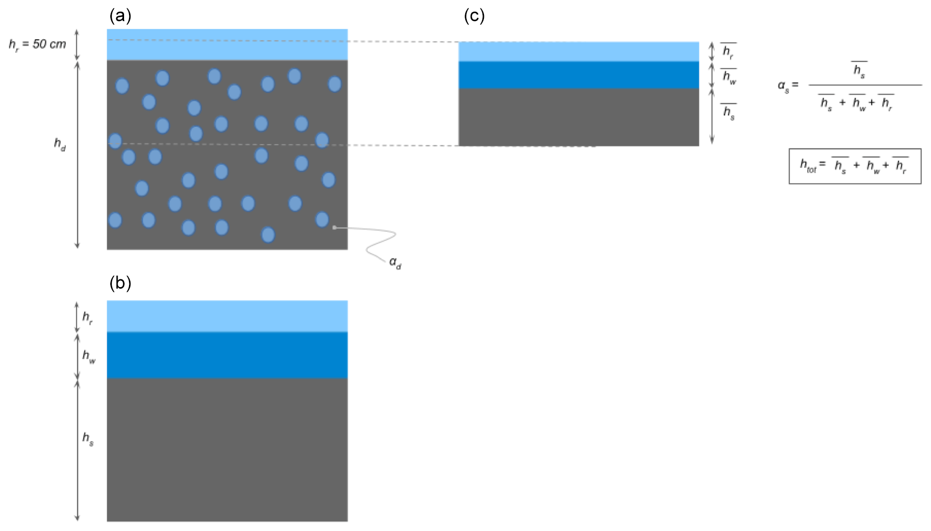
Figure 6 Definition of the variables used to define the initial thickness mobilizable h_tot. (a) The water-saturated deposit of thickness h_d, with porosity α_d, and the layer of rainwater available of maximum thickness h_r=50 cm (assumed). (b) Same as in (a) but if we imagine extracting all the pore-filling water and separating it into a layer of water of thickness h_w and a layer of compacted deposit of thickness h_s, which is the tephra fallout deposit simulated by the HAZMAP simulator in this study. (c) The thickness of the mobilizable layers of deposit ${\stackrel{\mathrm{‾}}{h}}_{\mathrm{s}}$, rainwater ${\stackrel{\mathrm{‾}}{h}}_{\mathrm{r}}$, and pore-filling water ${\stackrel{\mathrm{‾}}{h}}_{\mathrm{w}}$ depends on the availability of rain and deposits as well as the fixed solid fraction as of the initial flow.

The initial flow thickness that is remobilized, h_tot, will be the sum of three thicknesses:

• ${\stackrel{\mathrm{‾}}{h}}_{\mathrm{s}}\le h_{\mathrm{s}}$ from the solid part of the deposit,

• ${\stackrel{\mathrm{‾}}{h}}_{\mathrm{w}}\le h_{\mathrm{w}}$ from the water already filling the pores, and

• ${\stackrel{\mathrm{‾}}{h}}_{\mathrm{r}}\le h_{\mathrm{r}}$ from the rain (as said above, we assume h_r= 0.5 m).

There are relations linking these three addends. In particular, due to the condition of water saturation in the deposit,

$$\begin{array}{}\text{(21)}& {\mathit{\alpha }}_{\mathrm{d}}={\displaystyle \frac{{\stackrel{\mathrm{‾}}{h}}_{\mathrm{w}}}{{\stackrel{\mathrm{‾}}{h}}_{\mathrm{s}}+{\stackrel{\mathrm{‾}}{h}}_{\mathrm{w}}}}\end{array}$$

so that

$$\begin{array}{}\text{(22)}& {\stackrel{\mathrm{‾}}{h}}_{\mathrm{w}}={\displaystyle \frac{{\mathit{\alpha }}_{\mathrm{d}}}{(\mathrm{1}-{\mathit{\alpha }}_{\mathrm{d}})}}{\stackrel{\mathrm{‾}}{h}}_{\mathrm{s}}.\end{array}$$

Moreover, in the initial flow volume there is a relationship between water and solid content in terms of initial volumetric fraction α_s:

$$\begin{array}{}\text{(23)}& {\mathit{\alpha }}_{\mathrm{s}}={\displaystyle \frac{{\stackrel{\mathrm{‾}}{h}}_{\mathrm{s}}}{{\stackrel{\mathrm{‾}}{h}}_{\mathrm{s}}+{\stackrel{\mathrm{‾}}{h}}_{\mathrm{w}}+{\stackrel{\mathrm{‾}}{h}}_{\mathrm{r}}}}\end{array}$$

so that (combining Eq. 22)

$$\begin{array}{}\text{(24)}& {\stackrel{\mathrm{‾}}{h}}_{\mathrm{r}}={\displaystyle \frac{(\mathrm{1}-{\mathit{\alpha }}_{\mathrm{s}})}{{\mathit{\alpha }}_{\mathrm{s}}}}{\stackrel{\mathrm{‾}}{h}}_{\mathrm{s}}-{\displaystyle \frac{{\mathit{\alpha }}_{\mathrm{d}}}{\left(\mathrm{1}-{\mathit{\alpha }}_{\mathrm{d}}\right)}}{\stackrel{\mathrm{‾}}{h}}_{\mathrm{s}}={\displaystyle \frac{\mathrm{1}-{\mathit{\alpha }}_{\mathrm{d}}-{\mathit{\alpha }}_{\mathrm{s}}}{{\mathit{\alpha }}_{\mathrm{s}}(\mathrm{1}-{\mathit{\alpha }}_{\mathrm{d}})}}{\stackrel{\mathrm{‾}}{h}}_{\mathrm{s}}.\end{array}$$

We see from Eqs. (22) and (24) that both ${\stackrel{\mathrm{‾}}{h}}_{\mathrm{w}}$ and ${\stackrel{\mathrm{‾}}{h}}_{\mathrm{r}}$ are linear functions of ${\stackrel{\mathrm{‾}}{h}}_{\mathrm{s}}$. Considering the initial availability of remobilizable deposits, we can state that

$$\begin{array}{}\text{(25)}& {\stackrel{\mathrm{‾}}{h}}_{\mathrm{w}}+{\stackrel{\mathrm{‾}}{h}}_{\mathrm{s}}\le h_{\mathrm{d}},\end{array}$$

or, using Eq. (22),

$$\begin{array}{}\text{(26)}& {\stackrel{\mathrm{‾}}{h}}_{\mathrm{s}}\le \left(\mathrm{1}-{\mathit{\alpha }}_{\mathrm{d}}\right)h_{\mathrm{d}}.\end{array}$$

Considering, on the other hand, the available water from rain, we have

$$\begin{array}{}\text{(27)}& {\stackrel{\mathrm{‾}}{h}}_{\mathrm{r}}\le h_{\mathrm{r}},\end{array}$$

or, using Eq. (24),

$$\begin{array}{}\text{(28)}& {\stackrel{\mathrm{‾}}{h}}_{\mathrm{s}}\le {\displaystyle \frac{(\mathrm{1}-{\mathit{\alpha }}_{\mathrm{d}}){\mathit{\alpha }}_{\mathrm{s}}}{(\mathrm{1}-{\mathit{\alpha }}_{\mathrm{d}})-{\mathit{\alpha }}_{\mathrm{s}}}}{h}_{\mathrm{r}}.\end{array}$$

The maximum solid thickness ${\stackrel{\mathrm{‾}}{h}}_{\mathrm{s}}$ that can be remobilized, considering the availability of water-saturated deposits and rain as well as the a priori sampled initial solid fraction α_s, is then the maximum satisfying both conditions in Eqs. (26) and (28), i.e.

$$\begin{array}{}\text{(29)}& {\stackrel{\mathrm{‾}}{h}}_{\mathrm{s}}\le \min \left\{{\displaystyle \frac{(\mathrm{1}-{\mathit{\alpha }}_{\mathrm{d}}){\mathit{\alpha }}_{\mathrm{s}}}{\mathrm{1}-{\mathit{\alpha }}_{\mathrm{d}}-{\mathit{\alpha }}_{\mathrm{s}}}}{h}_{\mathrm{r}};\left(\mathrm{1}-{\mathit{\alpha }}_{\mathrm{d}}\right)h_{\mathrm{d}}\right\}.\end{array}$$

Once this is known, we can get the total initial thickness of the lahar by simply computing it as

$$\begin{array}{}\text{(30)}& h_{\mathrm{tot}}={\displaystyle \frac{{\stackrel{\mathrm{‾}}{h}}_{\mathrm{s}}}{{\mathit{\alpha }}_{\mathrm{s}}}}.\end{array}$$

The ashfall deposit which does not contribute to the initial volume of the lahar is added to the pre-existing topography as an erodible layer. The contribution of the ashfall deposits in the intermediate and distal areas has been significant in past sub-Plinian eruptions, as shown in the paper by Di Vito et al. (2024).

The steps described above are represented in Fig. 7 for the real-topography test application to Valle di Avella from the identification of areas “prone” to remobilization on the basis of geomorphological features, e.g. the terrain slope (Fig. 7a, red pixels), to the application of the criterion in Eqs. (29) and (30) to compute the initial thickness of lahar (Fig. 7b) from the rainwater available and the ashfall deposit (top panel, contour lines). For the case presented in Fig. 7 we assumed a deposit porosity α_d=0.22 and an initial solid fraction in the lahar α_s=0.29. With these values, Eqs. (29) and (30) give, for an ashfall deposit thickness of 0.4 m and an amount of rain of 0.5 m, an initial lahar thickness of approximately 0.8 m.

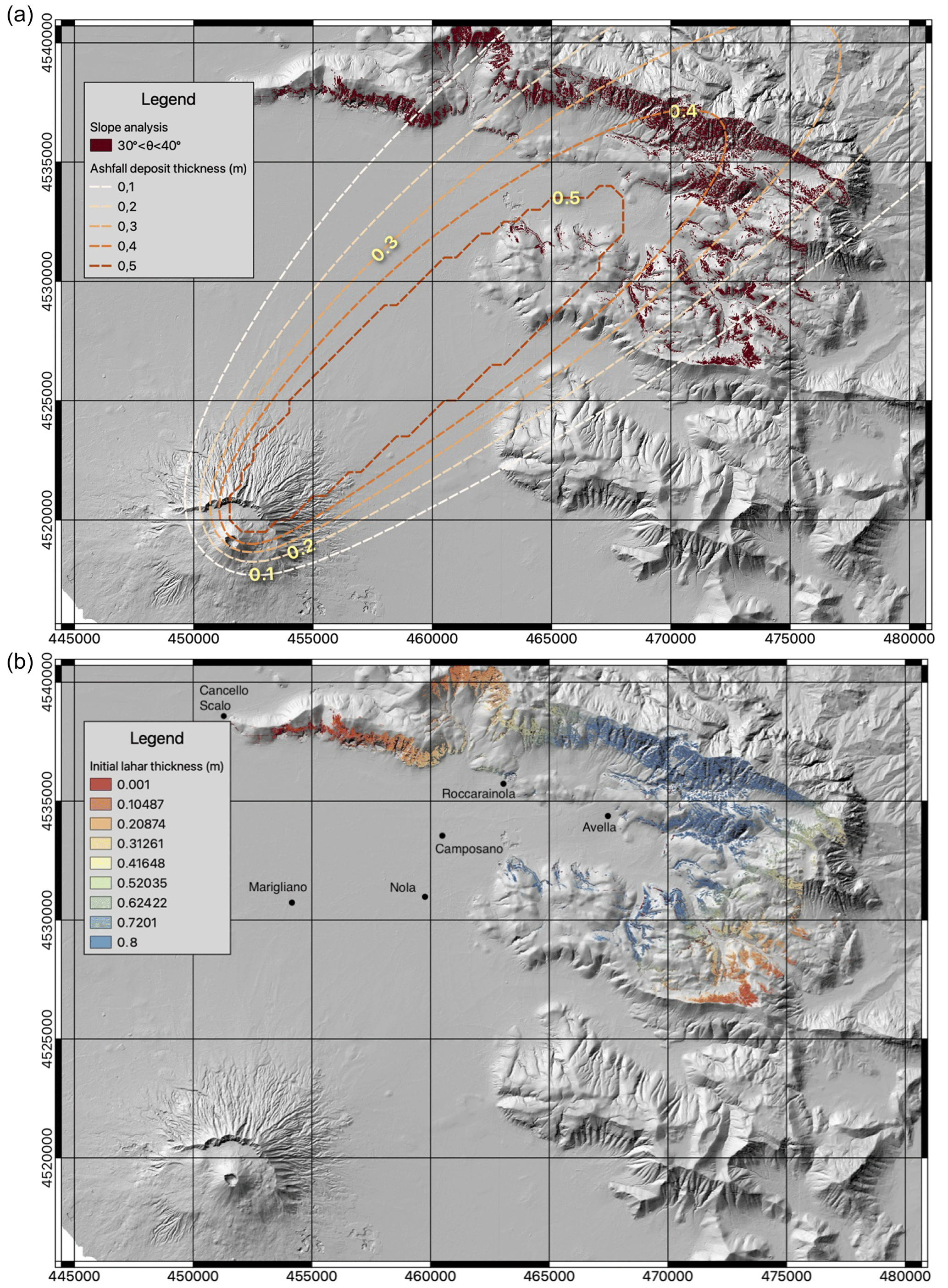
Figure 7 Steps for the definition of the initial lahar thickness. (a) Grid cells with a slope between θ_min and θ_max (red pixels) and the HAZMAP deposit thickness (contour lines). (b) The initial lahar thickness.

Concerning the grain size distribution of the remobilized deposits here we used that obtained by Di Vito et al. (2024) on the basis of field data analysis.

3.3 Application to real topography: sensitivity tests and description of the relevant output variables

We conduct a series of sensitivity tests on the real-topography test area in order to quantify the relevance of different terms and processes for the output of the simulations in terms of flow thickness and/or area.

We first present a reference simulation, extracted from the ensemble of simulations presented in Sandri et al. (2024), and for this case we show the temporal evolution of the flow and the most relevant output produced by the model. Then, with respect to this simulation, we vary several parameters to show the sensitivity of the results to several model parameters. For all the simulations presented in this analysis we used a value $\mathit{ϵ}={\mathrm{10}}^{-\mathrm{4}}$ m⁻¹ for the erosion coefficient (Eq. 14).

3.3.1 Flow evolution and relevant output

In this section we describe a reference simulation, obtained for a computational grid with cells of 50 m and a second-order numerical scheme in space, by applying a van Leer slope limiter to the reconstruction of the flow variable. For this simulation, the total grain size distribution is discretized with six bins from $\mathit{\varphi }=-\mathrm{3}$ to $\mathit{\varphi }=-\mathrm{7}$, and we assume an initial temperature of the lahar of 373 K. While we recognize that this temperature is more adequate for syn-eruptive lahars from pyroclastic density current deposits, here we used this value to better show the effect of the temperature on the lahar dynamics. In fact, later in the paper, we compare the results with those obtained with a colder lahar (300 K).

The initial thickness of the lahar is shown in the bottom panel of Fig. 7, and its temporal evolution is presented in the four panels of Fig. 8. After 1 h from the mobilization (Fig. 8a) the lahar already invaded a large portion of the Valle di Avella, with its maximum thickness reaching a few metres in its southern part and a thickness of a few millimetres still moving on the flanks of the Apennines facing the valley. At this time, the lahar has already reached the localities of Avella, Roccarainola, and Camposano, which all are inside the case-study valley, while after 2 h the lahar has reached the city of Nola, just outside the valley. After 12 h of flow time, the lahar has already reached the localities of Marigliano and Cancello Scalo, the first being in the more open plain, while the second is near the WNW Apennine sector of the valley. After 24 h of flow time, the lahar has already reached the city of Acerra in the open plain. Although this simulation is not aimed at reproducing a particular event from the past, but at showing the model's ability to describe the different phenomena that may characterize a future lahar in the Avella Valley, it is interesting to note that these extents are corroborated by some historical sources on the events of the 1631 eruption, for which it is reported that the localities of Marigliano and Nola were reached by lahars, and by geological pieces of evidence reported in Di Vito et al. (2024).

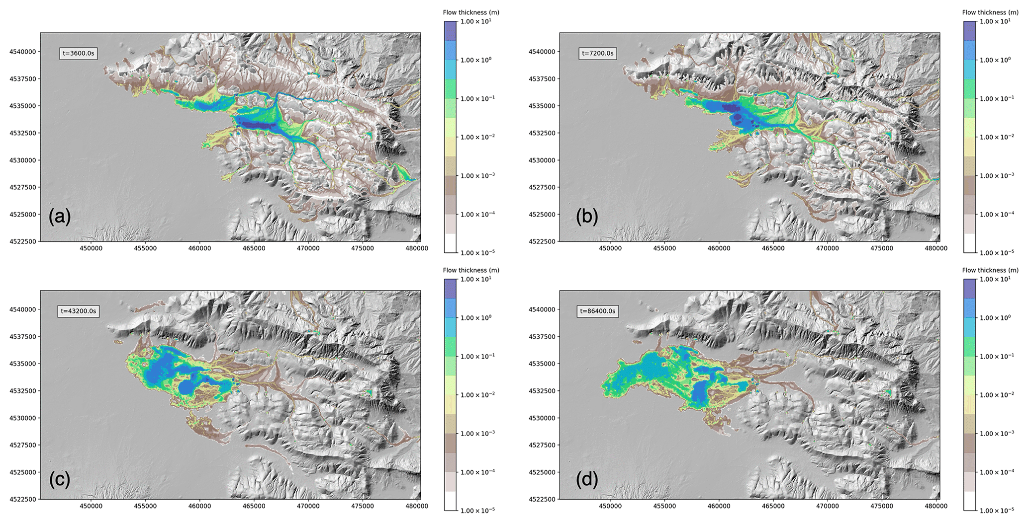
Figure 8 Lahar thickness temporal evolution: (a) 3600 s, (b) 7200 s, (c) 43 200 s, and (d) 86 400 s.

The area invaded by the lahar changes with time and its evolution is presented in Fig. 9. The model computes at each time step the invaded area as the sum of the areas of the grid cells where flow thickness is greater than a fixed threshold. For this analysis, two thresholds on the minimum flow thickness have been applied: a “physical” threshold set to 10⁻³ m (represented in Fig. 9 by the solid blue line), which allows us to analyse the dynamics of the bulk of the lahar, and a “numerical” threshold set to 10⁻⁵ m (represented by the dashed red line). It is important to remark that such a small threshold does not correspond to a thickness for which the flow is properly described by our model equations because for such values forces like surface tension become larger than gravity and friction (Hong et al., 2016). In any case, this small threshold can provide information on the dynamics of the very thin tail of the lahar, where the velocity goes rapidly to zero because of friction forces. Figure 9 shows that, for the larger physical threshold, at the beginning of the simulation (first 15 min) there is a rapid decrease in the area due to the channelization phase of the flow mobilized from the flanks of the Apennines. After this initial phase, the flow reaches the Valle di Avella and starts to spread out, with the area of the lahar increasing with time. For the lower thickness threshold, we observe that the area rapidly increases during the initial slumping phase of the lahar and reaches its maximum approximately 1 h after the mobilization. Then it decreases, first rapidly and then more slowly, increasing again after 15 h. This is due to the fact that tail of the flow gets thinner with time, and, as previously described, the presence of the yield strength term in the friction allows the flow to stop with a thickness that depends on the slope of the topography and on the fraction of solid material left in the flow. Thus, when the thickness is small enough, the tail of the lahar slows down and stops moving. Because of that, erosion becomes negligible and at the same time deposition occurs, further increasing the thinning of the deposit and the loss of sediments and water by the flow. This is shown well by the evolution of flow thickness on the flanks of the Apennines, as illustrated in Fig. 8. After 1 h from the mobilization, thickness is less than 1 mm, and, for the slope of the Apennines and the water content of the flow, this value is well below the critical thickness (see Fig. 3). Because of that, the flow stops moving and the only process occurring is the loss of water and sediments.

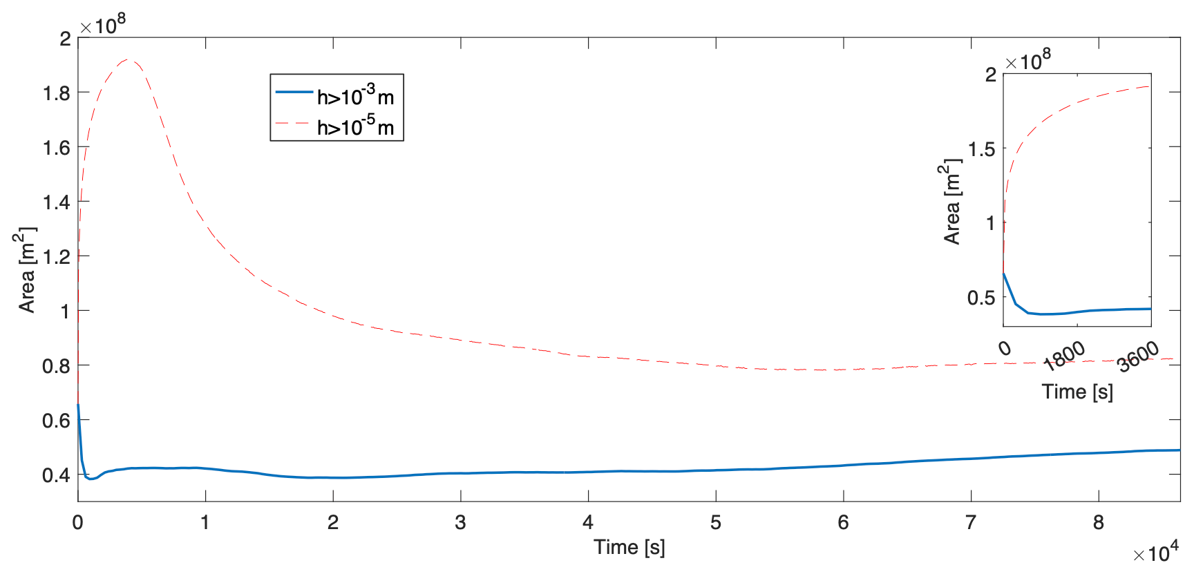
Figure 9 Area of the lahar versus time for the reference simulation. For the computation of the area two thresholds on thickness have been applied: a physical one (solid blue line, $h\ge {\mathrm{10}}^{-\mathrm{3}}$ m) and a numerical one (dashed red line, $h\ge {\mathrm{10}}^{-\mathrm{5}}$ m). The inset represents a detail of the first hour of simulation.

The mobility of the flow is mostly controlled by the solid fraction within the lahar, and this fraction can change because of erosion and deposition. Thus, the total erosion and deposition are important factors controlling the area invaded by the lahar. The final deposit and erosion thicknesses are presented in the left and right panels of Fig. 10, respectively, showing significant erosion where the flow is channelized, reaching a maximum value of a few decimetres. Conversely, deposition mostly occurs in the flat areas invaded by the lahar where the flow slows down, producing a maximum deposit thickness of the order of 1 m.

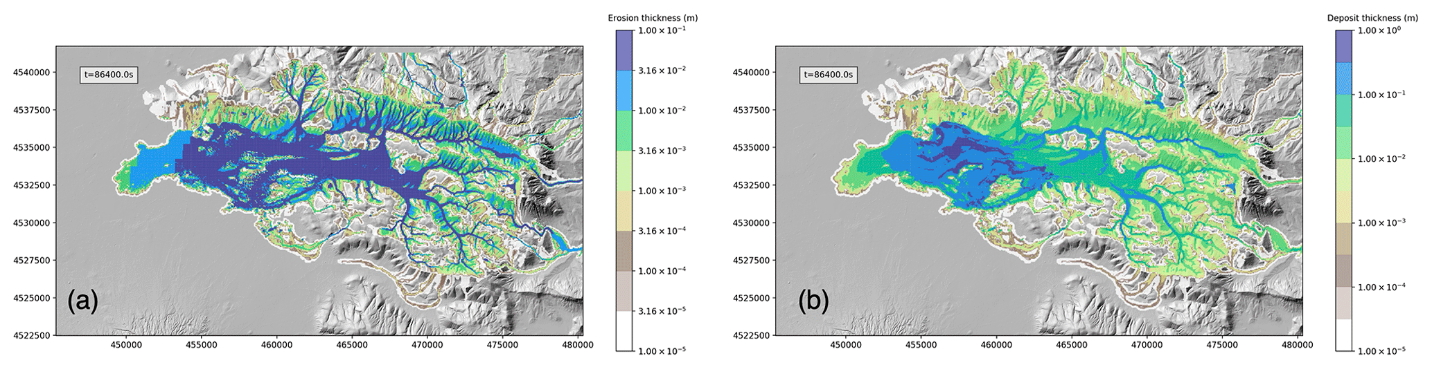
Figure 10 Total deposition (a) and erosion (b) after 24 h of simulation.

As shown by Eq. (17), deposition is proportional to the settling velocity of the sediments, which increases with their sizes. This is reflected in different depositional patterns for the different classes of particles, shown in the panels of Fig. 11. We observe that the thickness of the deposit for the different classes depends not only on the settling velocities, but also on the quantity of sediments available for deposition and thus on the initial grain size distribution of the lahar. This explains why the larger contribution to the deposit is given by class ϕ=5, for which the maximum thickness deposit 24 h after the mobilization of the lahar is about 1 m. For classes $\mathit{\varphi }=-\mathrm{3}$ and $\mathit{\varphi }=-\mathrm{1}$ the initial mass fractions are similar, and the difference in the final deposit is mostly due to the differences in settling velocities. In fact, Fig. 4 shows that, for the same total solid volume fraction of the lahar, a difference in size in the Krumbein scale of 2ϕ results in a difference in the settling velocity, and thus in the deposition rate, of 1 order of magnitude.

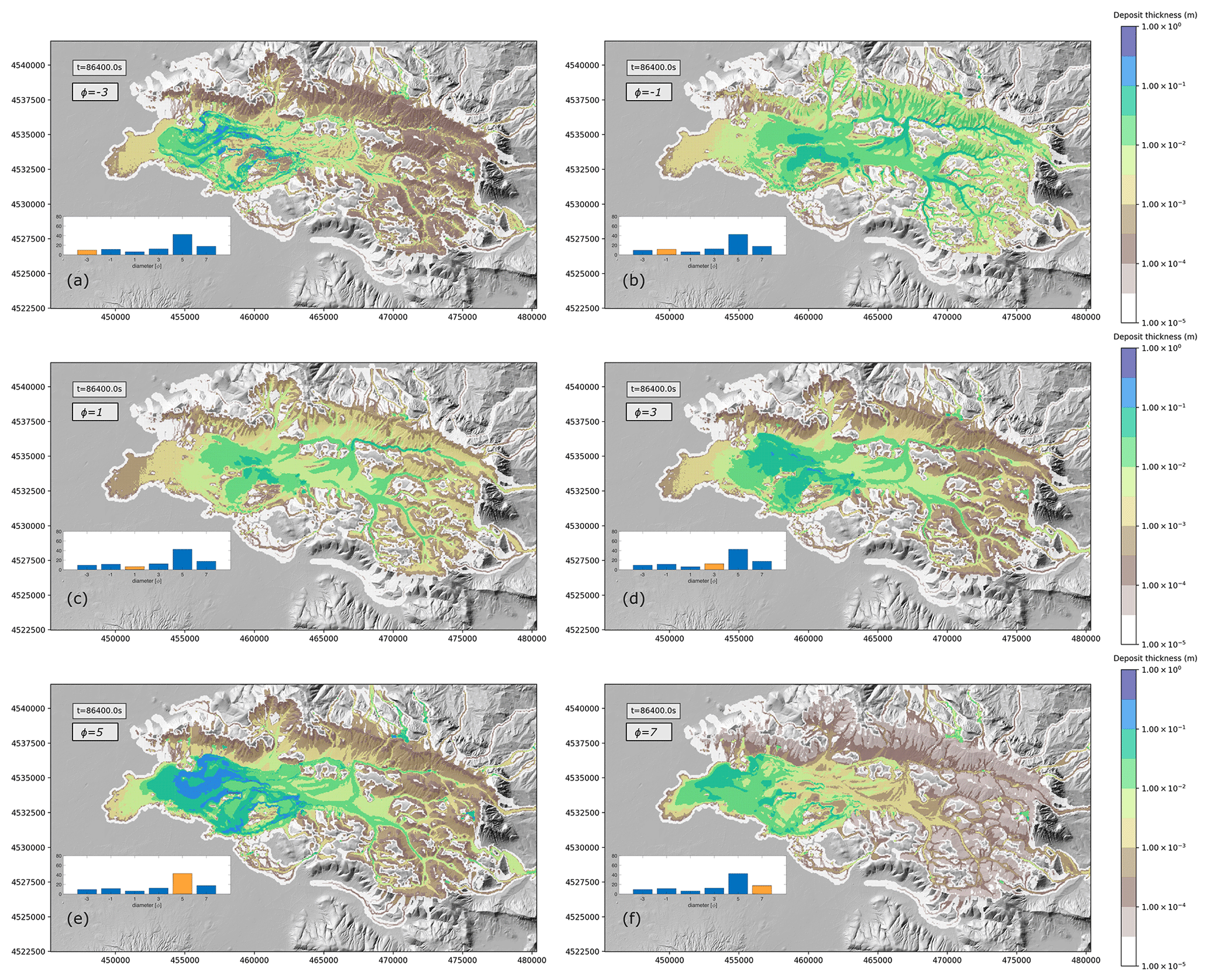
Figure 11 Total deposit thickness after 24 h of simulation for the six different classes of particles: (a) $\mathit{\varphi }=-\mathrm{3}$, (b) $\mathit{\varphi }=-\mathrm{1}$, (c) ϕ=1, (d) ϕ=3, (e) ϕ=5, and (f) ϕ=7. The insets in each panel show the initial total grain size distribution of the lahar, and the class for which the deposit is shown in the panel is represented in orange.

From the perspective of hazard assessment, it is not the flow thickness at the end of the simulation (here 24 h after the mobilization) that is important but rather the maximum thickness registered at each location reached by the lahar in the same time span, as shown in Fig. 12. This figure shows that the maximum thickness can exceed several metres over a large area of the domain, allowing us to identify the areas where the hazard is significant. Flow thickness may also be combined with dynamic pressure in order to assess, for different couples of thickness and dynamic pressure thresholds, the areas where these thresholds are exceeded simultaneously. Figure 13 shows, for two different thickness thresholds, the values of dynamic pressure exceeded during 24 h of simulation. For example, in Fig. 13b, the light green pixels represent the area where at some time the lahar produced, simultaneously, a thickness of at least 2 m and a dynamic pressure larger than 2000 Pa and smaller than 5000 Pa.

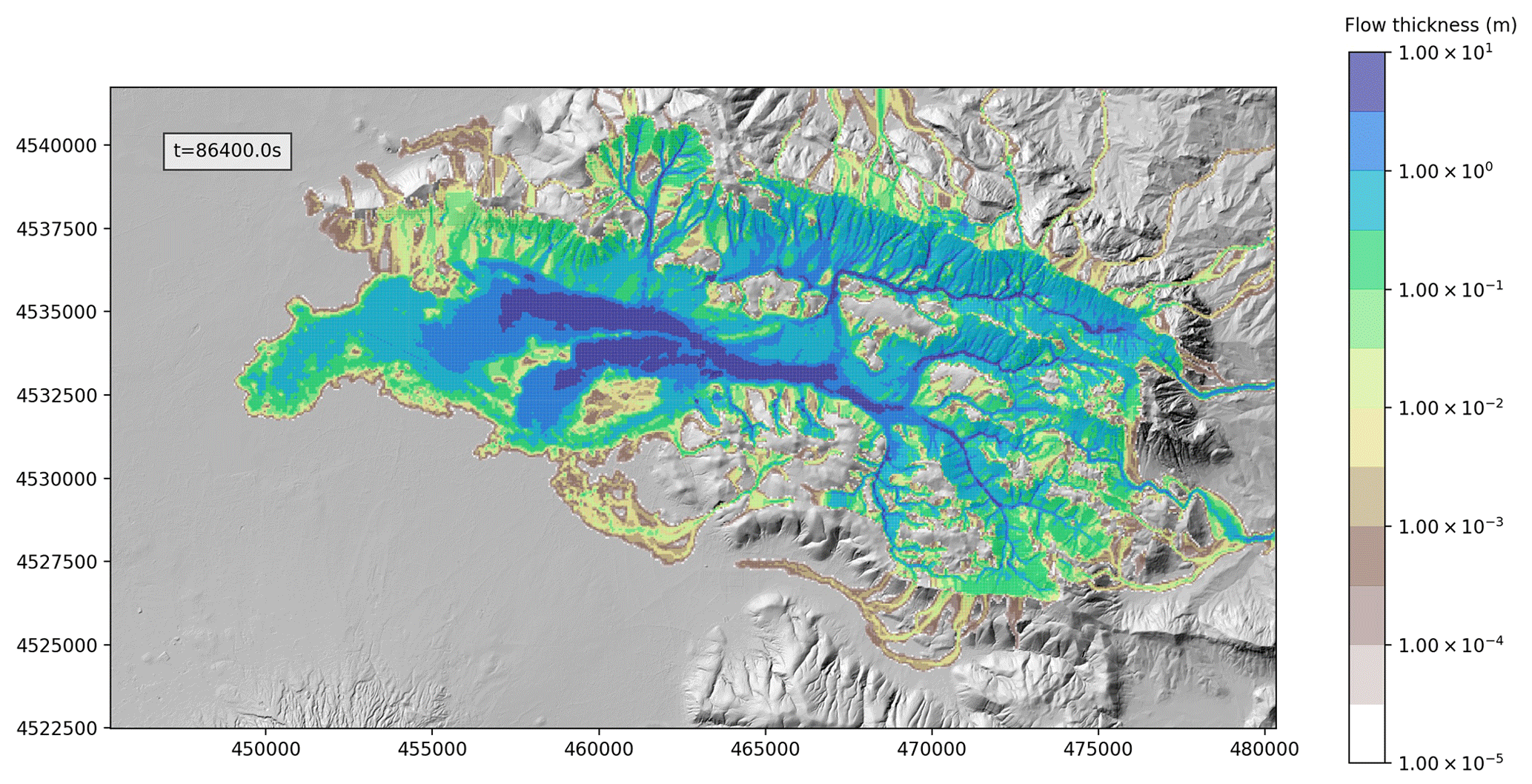
Figure 12 Maximum thickness of the flow in each cell of the computational grid during the 24 h of simulation.

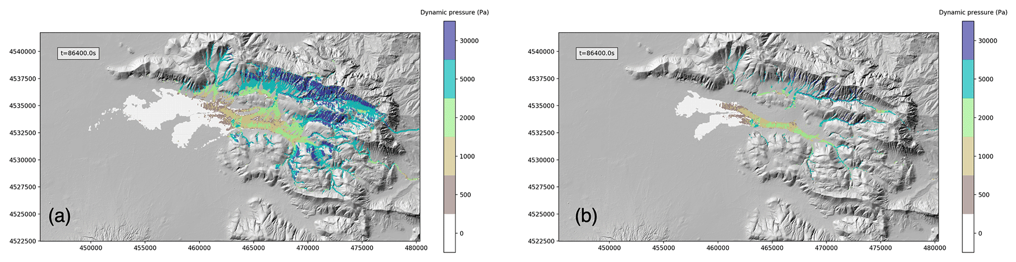
Figure 13 Maps of exceedance of flow thickness and dynamic pressure: (a) thickness threshold 0.5 m and (b) thickness threshold 2 m. The colours represent the dynamic pressure thresholds exceeded during the 24 h of simulation simultaneously with the thickness threshold.

3.3.2 Effects of grid size and numerical scheme order

In this section we want to present the effects of the resolution of the computational grid and of the spatial numerical scheme adopted (first- and second-order schemes). We remind the reader that the DEM resolution used for the simulations is 10 m, while the computational grid resolution used for the reference simulation presented in the previous section was 50 m. Thus, the smaller topographical features present in the original DEM are smoothed in the computational grid, possibly with an effect on the dynamics of the simulated flow. Here, we focus our interest on the first 2 h of the simulation and thus on the phase where the details of the topography can be more important because of the important canalization effects acting on the lahar when moving down the flanks of the Apennines into the Valle di Avella. All the simulations for this analysis have been performed on 16 cores of a multicore shared memory server SuperMicro 4 × 16-core AMD with 2.3 GHz.

In Fig. 14 we compare the flow thickness of the reference simulation (Fig. 14a) with a simulation obtained with a 100 m resolution computational grid (Fig. 14b), a simulation obtained with a 25 m resolution computational grid (Fig. 14c), and a simulation with a 50 m resolution computational grid but with a first-order spatial scheme (Fig. 14d). While there is a remarkable difference in the area invaded by the flow between the reference 50 m simulation and the 100 m simulation, the difference between the reference simulation and the 25 m one, in particular for significant flow thicknesses, is very small. We also have to account for the fact that, theoretically, the computational time required for a simulation when the grid cell size is decreased by a factor of 2 increases by a factor of 2³. In fact, the number of horizontal cells increases by a factor of 2², with the simulation being two-dimensional, and the time step decreases by a factor of 2 due to the well-known linear relationship between the spatial and temporal step associated with the use of an explicit integration scheme (CFL condition, Courant et al., 1928). In addition to this, the CPU time required for the initialization of the arrays and for the input–output procedures must be accounted for. For this particular case, the 100, 50, and 25 m resolution simulations required 1023, 6916, and 50 289 s, respectively. This suggests that, with the DEM we used, a 50 m resolution is adequate for a proper description of the flow dynamics, also in view of the utilization of the simulations for hazard studies, where a large number of runs is required and the computational time is an important constraint.

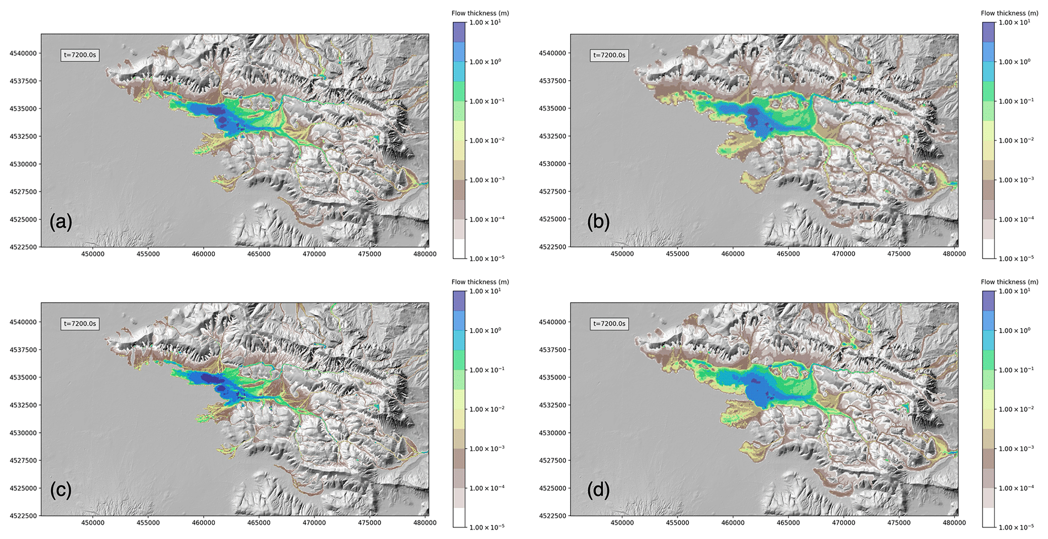
Figure 14 Maps of flow thickness at t= 7200 s for simulations with different grids or different numerical schemes: (a) 50 m grid resolution and second-order scheme with geometric limiter, (b) 100 m grid resolution and second-order scheme with geometric limiter, (c) 25 m grid resolution and second-order scheme with geometric limiter, and (d) 50 m grid resolution and first-order scheme (no geometric limits used).

Finally, in the bottom-right panel of Fig. 14, we can see the output of a simulation with the same resolution as the reference one (50 m), but without the use of geometric limiters for the linear reconstruction of flow variables at the interfaces of the computational cells. This makes the discretization scheme of first order, with respect to the second order obtained for the reference simulation. The difference in the results is striking, with the first-order simulation being more similar to the simulation obtained with the 100 m grid and the second-order simulation being similar to that obtained with the 25 m grid. The computational overhead associated with the use of geometrical limiters is small (6916 s vs. 6770 s), and thus their use is strongly suggested for this kind of simulation.

3.3.3 Effects of grain size discretization

In this section we present the sensitivity of model results to the discretization of grain size distribution. With respect to the reference simulation, where 6 classes were used, here we compare the solution after 4 h from the mobilization of the lahar with those at the same time for two simulations with the total grain size distribution described by 3 and 12 particle size classes, respectively. The results of this analysis are presented in Fig. 15, with the final flow thickness presented in the left panels and the deposit thickness in the right panels. The plots show small differences between the simulations with 3 (Fig. 15a–b) and 6 classes (Fig. 15c–d), which become almost negligible when comparing the simulations with 6 and 12 classes (Fig. 14e–f). For this test case, the increase in the number of classes from 6 to 12 resulted in an increase in the computational time of a factor of 1.3. Thus, the choice of using six classes for the reference simulations represents a good compromise between accuracy and efficiency.

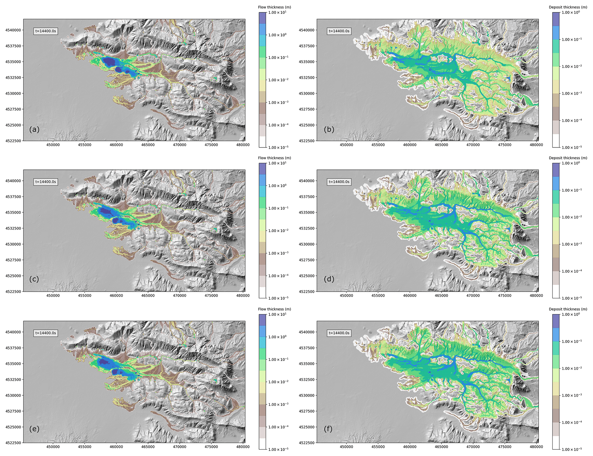
Figure 15 Maps of flow thickness (a, c, e) and deposit thickness (b, d, f) at t= 14 400 s for simulations with different discretizations of the total grain size distribution: (a–b) 3 classes, (c–d) 6 classes, and (e–f) 12 classes.

3.3.4 Effect of initial temperature

In this section we present a comparison between the output of the reference simulation (T= 373 K) and a simulation with a lower initial temperature (T= 300 K).

Figure 16 shows the invaded area (computed as the sum of the areas of the grid cells where flow thickness is greater than or equal to 10⁻³ m) versus time for the two simulations, where the result for the reference simulation is presented with a red line, while the result for the colder case is plotted with a blue line. We remark that here we are not plotting the area of the deposit of the lahar, but the area where the lahar is still moving, in order to better understand how flow viscosity affects the dynamics of the flow. In the initial phase (< 60 s), the difference between the two cases is negligible, while it becomes more significant with time, with the area of the colder flow exceeding that of the reference one. This can seem counterintuitive because we expect an increased mobility for the hotter flow due to the lower viscosity and thus a larger runout. But the initial phase is dominated by flow channelization, which is increased by the larger mobility and which results in a smaller footprint of the lahar. The different viscosity of the flow also affects the tail of the flow in a twofold way. Indeed, the lower viscosity results in a larger settling velocity of the sediments and a debulking which further increases the flow mobility. This is evident by looking at the reduced footprint of the flow left on the Apennines flanks in the simulation with the higher initial temperature (Fig. 14a) with respect to the simulation with the lower initial temperature (Fig. 17).

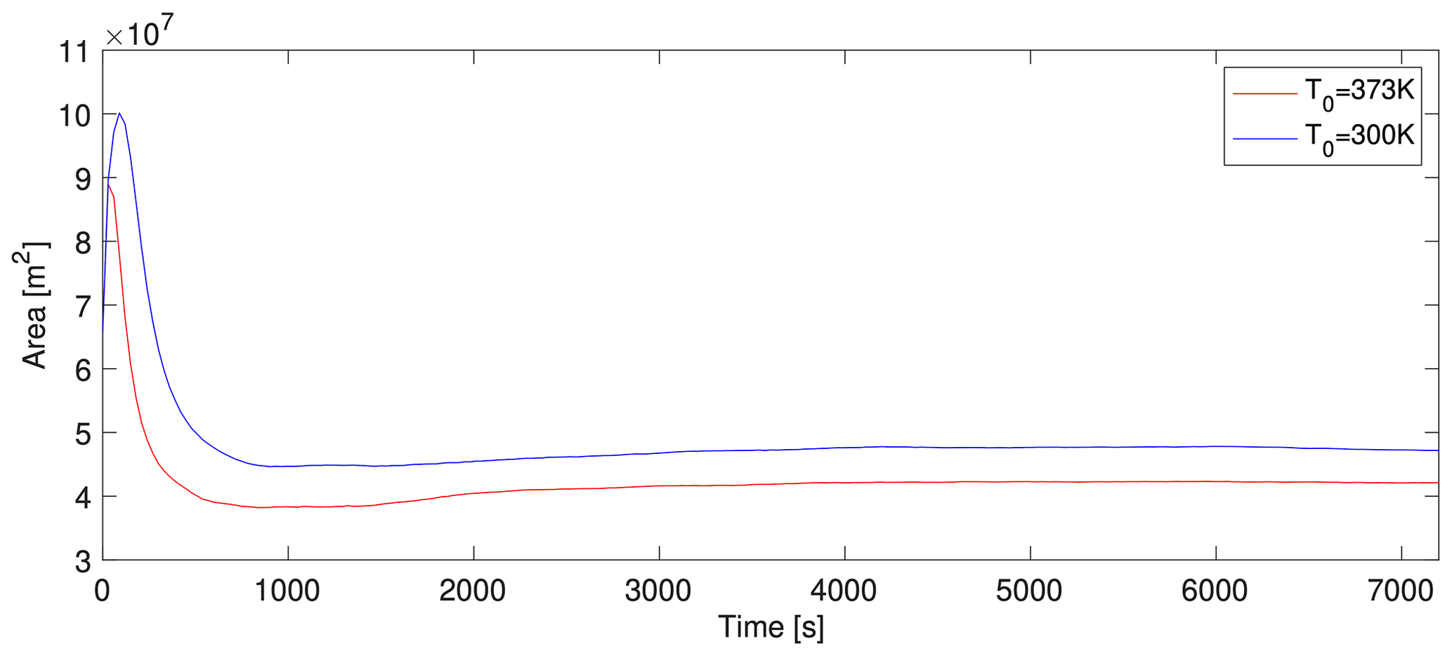
Figure 16 Area of the lahar versus time for the simulations with different initial temperatures: 300 K (blue line) and 373 K (red line). The area is computed as the sum of the areas of the grid cells where flow thickness is greater than 10⁻³ m.

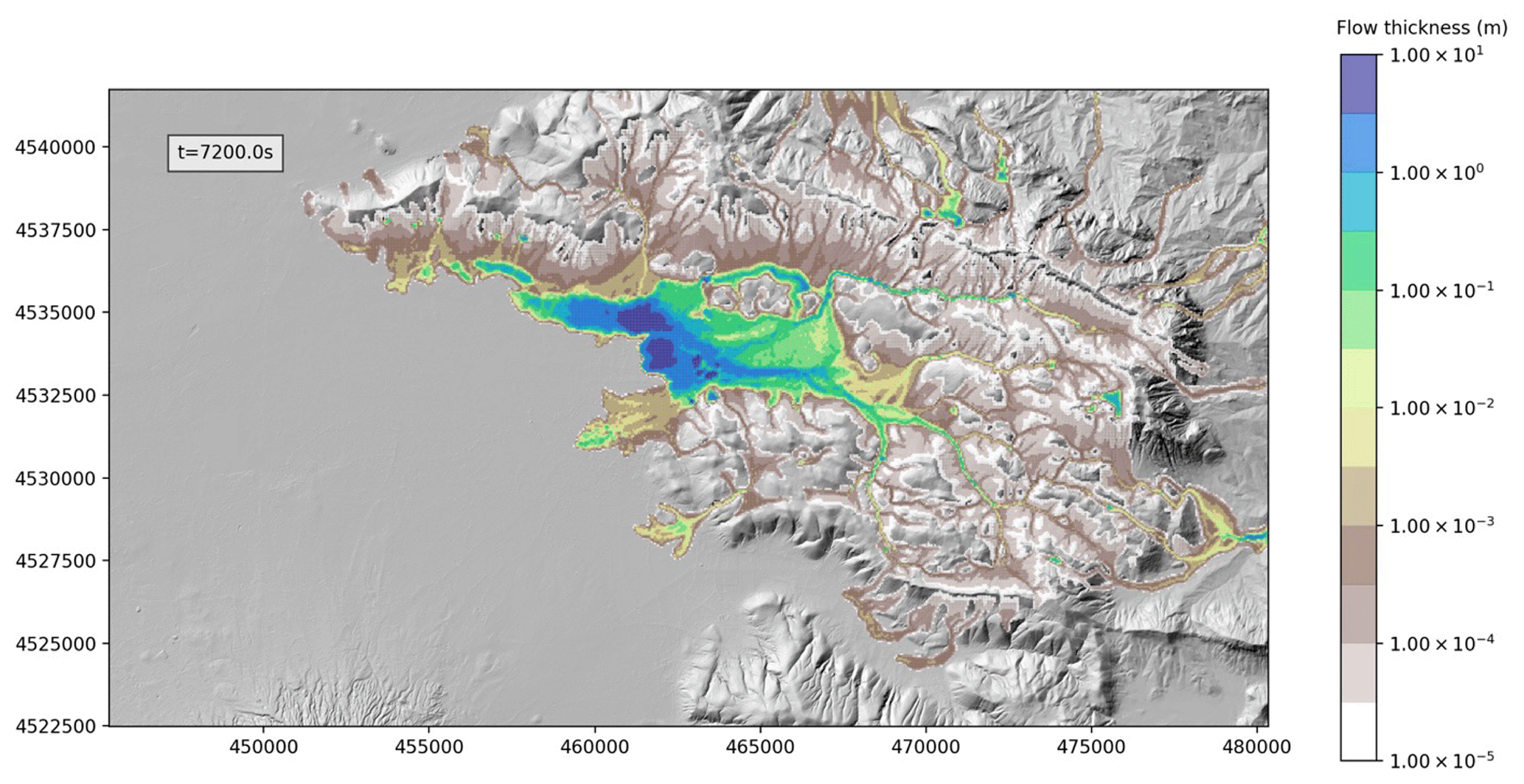
Figure 17 Maps of flow thickness at t= 7200 s for a simulation with an initial temperature T= 300 K.

3.3.5 Effects of erosion and deposition

As shown in the previous comparison, the viscosity of the flow has an effect on the debulking process, which in turn can affect the lahar propagation. Here we focus our attention on the effects of the main processes controlling lahar bulking and debulking, i.e. the deposition and erosion processes.

This is done by comparing in Fig. 18 the first 2 h of the reference simulation (Fig. 18a) with three additional test cases: a simulation without erosion (Fig. 18b), a simulation without deposition (Fig. 18c), and a simulation without erosion and deposition (Fig. 18d).

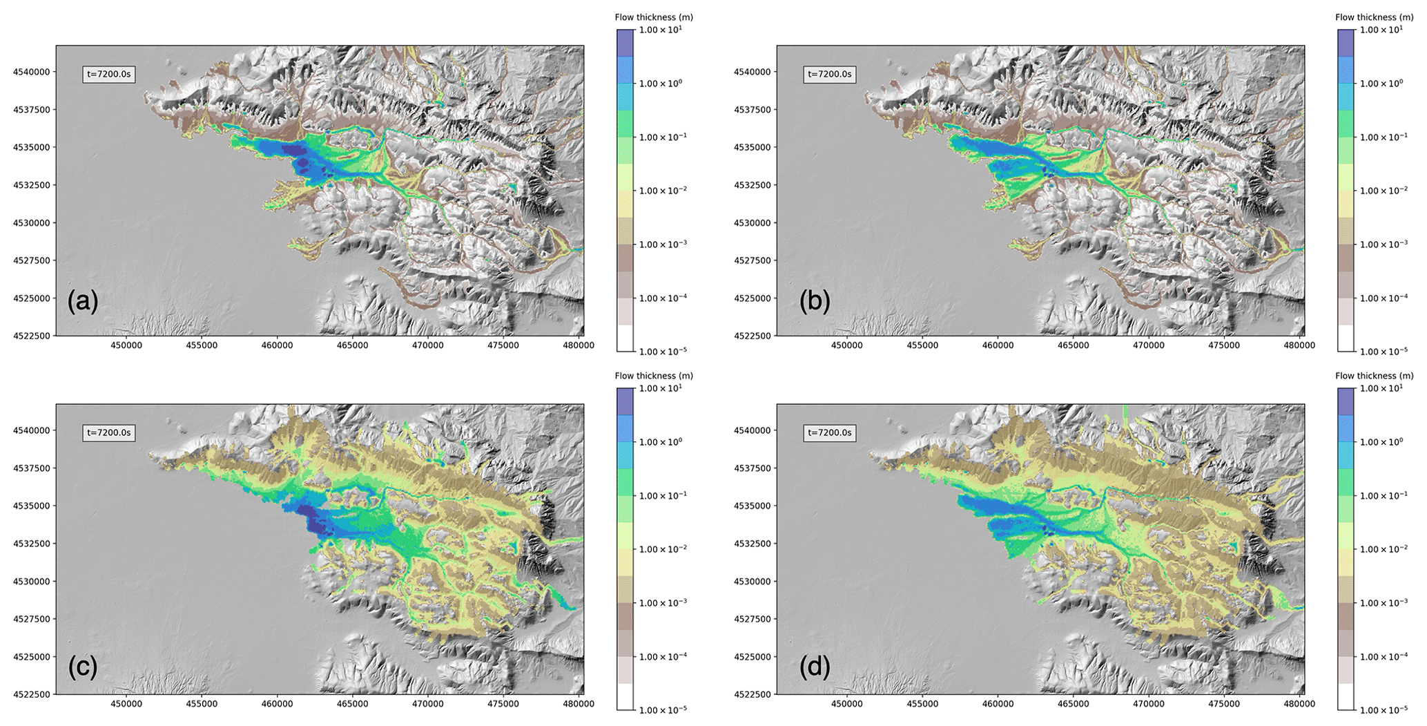
Figure 18 Maps of flow thickness at t= 7200 s for simulations with and without erosion and deposition: (a) reference simulation with erosion and deposition, (b) simulation with deposition and without erosion, (c) simulation with erosion and without deposition, and (d) simulation without erosion and deposition.

By comparing the flow thickness and the area covered by the flow of the reference simulation and that without erosion, we can see the twofold effect of the bulking associated with erosion. On one hand we observe the larger flow thickness; on the other hand, we observe a smaller runout due to the lower mobility associated with a higher solid volume fraction. This is particularly true in the Valle di Avella, where the front of the flow advanced about 2 km more for the simulation without erosion.

4 Conclusions

A new shallow layer model for describing lahar transport was presented. The proposed model does not describe all the general aspects of lahar behaviour (see Pudasaini, 2012) but contains the essential physics needed to reproduce the general features of lahars observed in nature, which is crucial for assessing their hazard.

In particular the model considers realistic particle size distribution as well as surface erosion and deposition processes through semi-empirical parameterizations calibrated from field data.

The model was developed with the aim of describing lahar propagation and deposits and assessing their hazard in contexts similar to that of the Vesuvius area, which is highly populated and prone to this kind of phenomenon after heavy rains (e.g. Fiorillo and Wilson, 2004).

The critical variables were identified and several sensitivity tests carried out using synthetic and real case topographies.

The variables used in order to define the source are the initial mobilizable thickness, the water-saturated deposit thickness, the layer of rainwater, and the thickness of compacted deposit, which is related to the others through the substrate porosity.

The steps used for the assessment of the initial lahar thickness were presented for the real-topography test application to Valle di Avella.

The comparisons of simulations obtained for different numerical grids (from 25 to 100 m), scheme order, and grain size discretization were useful to find a good compromise between resolution and computational speed. The DEM used, however, was at a resolution (10 m) finer than that of the computational grid.

The friction term is defined as the sum of a velocity-independent yield slope, a viscous slope, and turbulent slope (O'Brien et al., 1993). The yield strength and the fluid viscosity are considered functions of the total solid volumetric fraction in a consistent way. The values of the three terms strongly depend on volumetric solid fraction, flow thickness, and velocity. They can vary in a non-linear way by several orders of magnitude when thickness, velocity, and solid fraction vary in ranges typical for lahars. This can produce a stiff term in the system of equations, and, for this reason, a robust solver is needed that allows coupling between the gravitational and frictional terms to be accurately simulated.

Energy transport and temperature effects were also explored in order to better understand how flow viscosity affects the dynamics of the flow. When the friction is dominated by the yield slope term, the difference between the high- and low-temperature cases is negligible, while it becomes more significant with time, with the area of the colder flow exceeding that of the cold one. In fact, the lower viscosity in the case of the hot flow, besides increased mobility, also results in a larger settling velocity of the sediments and a debulking which further increases the flow mobility, producing a reduced footprint deposit area of the flow.

Effects of erosion and deposition were investigated by comparing the simulations (i) without erosion, (ii) without deposition, (iii) without erosion and deposition, and (iv) with erosion and deposition. By comparing flow thickness and area covered by the flow, we can see the twofold effect of the bulking associated with erosion that consists of larger flow thicknesses and smaller runouts due to the lower mobility associated with higher solid volume fractions.

The companion paper by Sandri et al. (2024) will show an application of the presented model for hazard analysis of lahars from Vesuvius deposits in the Neapolitan area, where a wide range of initial conditions are investigated to produce probabilistic hazard maps. To reach this goal, the companion paper considers 11 hydraulic catchments threatening the Campanian Plain, and in each catchment a large number of simulations accounts for the variability in the initial lahar volume, initial water fraction, and initial mass load of the ashfall deposit. The database of simulations considered in the analysis by Sandri et al. (2024) would allow one to also consider alternative realizations of the events of the 1631 eruption, permitting a counterfactual analysis that can be very insightful for lahar risk analysis (Aspinall and Woo, 2019), and it will be the focus of future research.