Statistical appraisal of geothermal heat flow observations in the Arctic

Geothermal heat flow is an important boundary condition for ice sheets, affecting, for example, basal melt rates, but for ice-covered regions, we only have sparse heat flow observations with partly high uncertainty of up to 30 m W m⁻². In this study, we first investigate the agreement between such pointwise heat flow observations and solid Earth models, applying a 1D steady-state approach to perform a statistical analysis for the entire Arctic region. We find that most of the continental heat flow observations have a high reliability and agreement to solid Earth models, except a few data points, such as, for example, the NGRIP (North Greenland Ice Core Project) point in central Greenland.

For further testing, we perform a conditional simulation with focus on Greenland in which the local characteristics of heat flow structures can be considered. Simple kriging shows that including or excluding the less reliable NGRIP point has a large influence on the surrounding heat flow. The geostatistical analysis with the conditional simulation supports the assumption that NGRIP might not only be problematic for representing a regional feature but likely is an outlier. Basal melt estimates show that such a local spot of high heat flow results in local high basal melt rates but leads to less variation than existing geophysical models.

1 Introduction

Geothermal heat flow (GHF) is a key factor of solid Earth–cryosphere interaction. Under ice-covered regions, such as Greenland, GHF is a boundary condition for ice sheet dynamics (Karlsson et al., 2021; Goodge, 2018). For example, Karlsson et al. (2021) state that GHF can contribute up to 25 % of total basal melt rates, while locally high heat flow can have a larger impact on ice sheet dynamics compared to a regionally higher value (McCormack et al., 2022). GHF itself is influenced by the solid Earth, first of all reflecting the thickness of the lithosphere (Lösing and Ebbing, 2021), as well as hydrological processes (Gooch et al., 2016) or crustal heat production variations (Bons et al., 2021), making heat flow for continental settings highly variable (Reading et al., 2022). Furthermore, maps of GHF are often based on interpolation of sparse observations, so isolated points might distort the distribution. However, geothermal heat flow is complicated to measure directly. Borehole measurements are expensive and therefore sparse in large parts of the Arctic (and Antarctic), which is covered with ice and snow most of the year. Additionally, observations are often concentrated in areas of economic interest or areas that are easily accessible (Stål et al., 2022). Therefore, Arctic heat flow observations are distributed very heterogeneously, with dense data coverage in regions around the mid-oceanic ridge, Scandinavia, and the north of Canada, while Siberia, Greenland, and the Arctic Ocean north of Alaska are poorly covered (Lucazeau, 2019; Fig. 2).

Ice temperature profiles present another option to estimate GHF in glacial areas (e.g., Dahl-Jensen et al., 2003). If the borehole reaches the ice–bedrock interface, GHF can be estimated using models of heat transport in the column of ice (e.g., Weertman, 1968; Rasmussen et al., 2013). However, not all boreholes reach the bedrock, so the ice temperature profiles need to be extrapolated (e.g., Kinnard et al., 2006; Buchardt and Dahl-Jensen, 2007), leading to large uncertainties for estimated heat flow values. The NGRIP (North Greenland Ice Core Project) point in central Greenland is a particularly notorious example (Buchardt and Dahl-Jensen, 2007), with a wide range of values between 63 m W m⁻² (for example, Martos et al., 2018) and 970 m W m⁻² (Smith-Johnsen et al., 2020) being suggested in the literature. The latter estimate is highly unlikely, but even the most conservative estimates well exceed the mean of Greenland with 60 m W m⁻² (Colgan et al., 2022).

In turn, estimating heat flow from geophysical data gives the possibility of overcoming the sparseness, although with the abovementioned uncertainty. For example, Curie depth estimates based on magnetic data are a classical tool to infer heat flow. For Greenland, heat flow was derived from Curie depth estimates based on satellite magnetic (Fox Maule et al., 2009) or aeromagnetic (Martos et al., 2018) compilations. Thermal models of the entire lithosphere can also be constrained by a variety of geophysical data sets (i.e., gravity and surface wave data), but these models typically lack lateral resolution within the crust (Afonso et al., 2019; Pasyanos et al., 2014; Fullea et al., 2021).

A more geostatistical approach is to compare proxies in a region with poorly known heat flow with similar proxies in regions with good coverage. Upper-mantle seismic velocity was one of the first proxies used to infer GHF (Shapiro and Ritzwoller, 2004), while Artemieva (2019) applied a thermal isostasy model. More recently, machine learning algorithms (specifically based on random forest regression) have been used to predict geothermal heat flow based on a variety of geographical/geophysical proxies (Colgan et al., 2022; Rezvanbehbahani et al., 2017; Lösing and Ebbing, 2021). See Colgan et al. (2022) for an extended discussion of GHF models for Greenland. However, such heat flow maps can only present regional heat flow, as they are limited by the availability and resolution of data. The non-linear optimization heuristic used in the machine learning techniques is also highly sensitive to isolated data points. Colgan et al. (2022) and Rezvanbehbahani et al. (2017) study this by omitting or varying the estimated GHF value for individual data points, respectively, and find that particularly the NGRIP point presents a challenge, as it is a highly uncertain and isolated measurement. But without additional information, local structures and regional features cannot be distinguished based on sparse point measurements. Heat flow anomalies can be as small as a few tens of kilometers due to shallow crustal heat production and the effect of subglacial topography (Reading et al., 2022). Thus, the interpolation (or random forest regression) of GHF observations is prone to large biases if local anomalies are mistaken for regional features. Nevertheless, local GHF anomalies are crucial for solid Earth–cryosphere interaction (McCormack et al., 2022).

In this study, we approach the question of local vs. regional effects on GHF from two angles. First, we evaluate a database of GHF measurements by testing each individual measurement's consistency with a lithospheric temperature model based on estimates of Moho and LAB (lithosphere–asthenosphere boundary) depths. Second, we use geostatistical analysis and conditional simulation to investigate the spatial scale of heat flow in Greenland. Our results can help decide whether to exclude points for interpolation and machine learning on a regional scale or in regions with sparse data, as they are not trustworthy for such applications.

2 Methods

For any heat flow observation, it is unknown whether the observed value reflects the regional setting or a local anomaly. Assuming that regional structures are in agreement with LAB and Moho depth models, it should be possible to find a set of thermal parameters (heat conductivity and heat productivity), such that GHF can be predicted from stationary 1D heat flow modeling (Lösing et al., 2020; Furlong and Chapman, 1987; Artemieva and Mooney, 2001). If no combination of the parameters within their given ranges lead to an agreement, the GHF observation should be considered suspicious or a local anomaly. For example, points in areas of exceptionally local high heat production from radiogenic sources (Bons et al., 2021) should lead to an incompatibility between the lithospheric model and GHF data.

We assume that geophysical LAB depth can be seen as a representation of the large-scale lithospheric temperature field, so we compare the predicted temperature at the LAB to an assumed LAB temperature of 1315 °C. If the temperature deviation surpasses a threshold of 100 K, we assume that the corresponding GHF observation probably is locally influenced and therefore cannot resolve the regional assumptions of the geophysical models. Choosing such high deviation, we take uncertainties from the used models for Moho and LAB depths into account.

We assume vertical heat flux within the lithosphere, which is a common assumption at least for the continental domain (Afonso et al., 2013; Lösing et al., 2020). Furthermore, the lithospheric columns are assumed to be in thermal equilibrium, resulting in the following temperature equation:

$$\begin{array}{}\text{(1)}& k_{\mathrm{1}}{\displaystyle \frac{{\partial }^{\mathrm{2}}T}{\partial z^{\mathrm{2}}}}=h\left(z\right),\end{array}$$

with the crustal thermal conductivity k₁, the temperature T, the depth z, and the heat productivity h.

Assuming no heat generation in the lithospheric mantle, the temperature increases linearly with depth, so that the temperature in the lithospheric mantle at a given depth can be calculated with

$$\begin{array}{}\text{(2)}& T\left(z\right)=T\left(M\right)+{\displaystyle \frac{q_{\mathrm{D}}}{k_{\mathrm{2}}}}(z-M),\end{array}$$

with the Moho depth M, the mantle heat flux q_D, and the mantle thermal conductivity k₂.

Heat production A is assumed constant with depth, following Lösing et al. (2020). The heat flux q at a certain depth is then

$$\begin{array}{}\text{(3)}& q\left(z\right)=q_{\mathrm{0}}-Az,\end{array}$$

where q₀ is the heat flux at the surface. When calculated at z=M, we get q_D.

For the temperature distribution in the crust we get

$$\begin{array}{}\text{(4)}& T\left(z\right)=T\left(\mathrm{0}\right)+{\displaystyle \frac{z{q}_{\mathrm{0}}-\frac{\mathrm{1}}{\mathrm{2}}A{z}^{\mathrm{2}}}{k_{\mathrm{1}}}}.\end{array}$$

Further derivations can be taken from Lösing et al. (2020).

The Moho temperature then can be determined by means of this temperature distribution; thus, a temperature at a certain depth in the lithospheric mantle is

$$\begin{array}{}\text{(5)}& T\left(z\right)=T\left(\mathrm{0}\right)+{\displaystyle \frac{M{q}_{\mathrm{0}}-\frac{\mathrm{1}}{\mathrm{2}}A{M}^{\mathrm{2}}}{k_{\mathrm{1}}}}+{\displaystyle \frac{q_{\mathrm{D}}}{k_{\mathrm{2}}}}(z-M).\end{array}$$

The mantle heat flux q_D can be calculated using Eq. (3). We now can use a Bayesian inversion coupled with a Monte Carlo Markov Chain (MCMC) algorithm to fit the heat flow observations to the temperature profile based on geophysical data and Eq. (5). This approach is based on the method presented in Lösing et al. (2020). The goal is to adjust a parameter vector so that the calculated model corresponds as closely as possible to the given model M (here the LAB temperature). For this purpose, Eq. (5) is used to define a forward operator F(Θ) that calculates the temperature at the LAB for a given parameter vector Θ. As a result, we also get estimates for the crustal and mantle thermal conductivity k₁ and k₂ and crustal heat production A. The principle of the algorithm is explained in Fig. 1.

Figure 1 Scheme of the MCMC algorithm as described in the text.

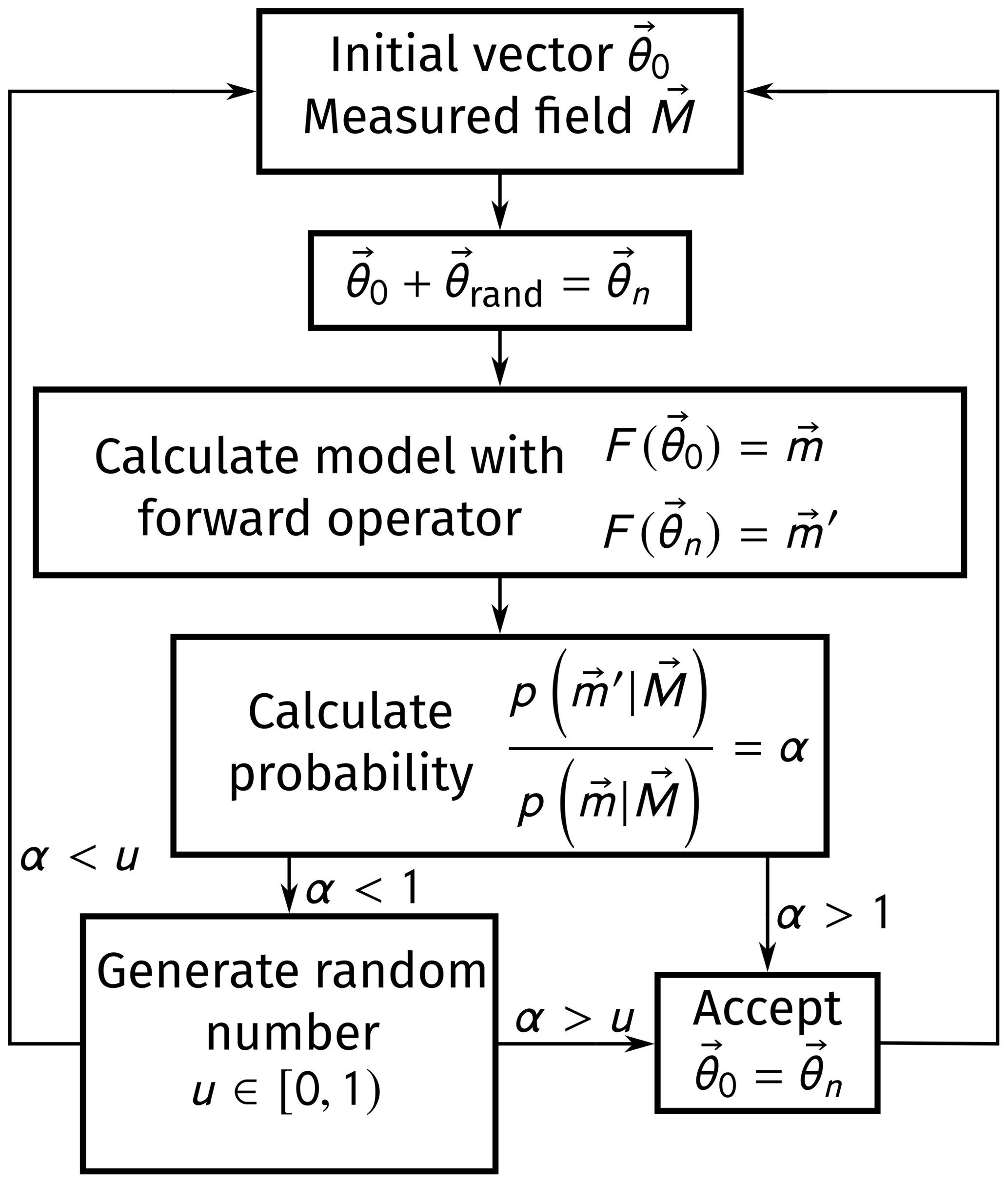
First, initial values for the thermal parameters are stored in a vector Θ. The forward operator now takes this vector and calculates a corresponding proposed model F(Θ)=m. A standard deviation of ${\mathit{\sigma }}_T^{\mathrm{2}}=\mathrm{100}$ K is allowed, due to uncertainties in the Moho and LAB depth models which were not precisely quantified – at least for the LAB depth (Afonso et al., 2019). The standard deviation is given by the relationship ${\mathit{\sigma }}_z={\mathit{\sigma }}_{T}k/q$ resulting in a few tens of kilometers of uncertainty for the input depths. For each iteration, we change the initial parameter vector Θ by adding random perturbations Θ_rand drawn from the so-called proposal distribution. We use a component-wise Gaussian distribution as proposal, which first randomly selects a thermal parameter to change and then perturbs this parameter by a value drawn from a zero-mean Gaussian distribution. The probability of a certain Θ depends on the prior distribution and the likelihood function (i.e., data fit) according to Bayes' law:

$$\begin{array}{}\text{(6)}& L\left(\mathit{M}\right|\mathbf{\Theta })=\prod _{i=\mathrm{1}}^N{\displaystyle \frac{\mathrm{1}}{\sqrt{\mathrm{2}\mathit{\pi }{\mathit{\sigma }}_M^{\mathrm{2}}}}}\exp -{\displaystyle \frac{{\left(F(\mathbf{\Theta }{)}_i-{\mathit{M}}_i\right)}^{\mathrm{2}}}{\mathrm{2}{\mathit{\sigma }}_M^{\mathrm{2}}}}.\end{array}$$

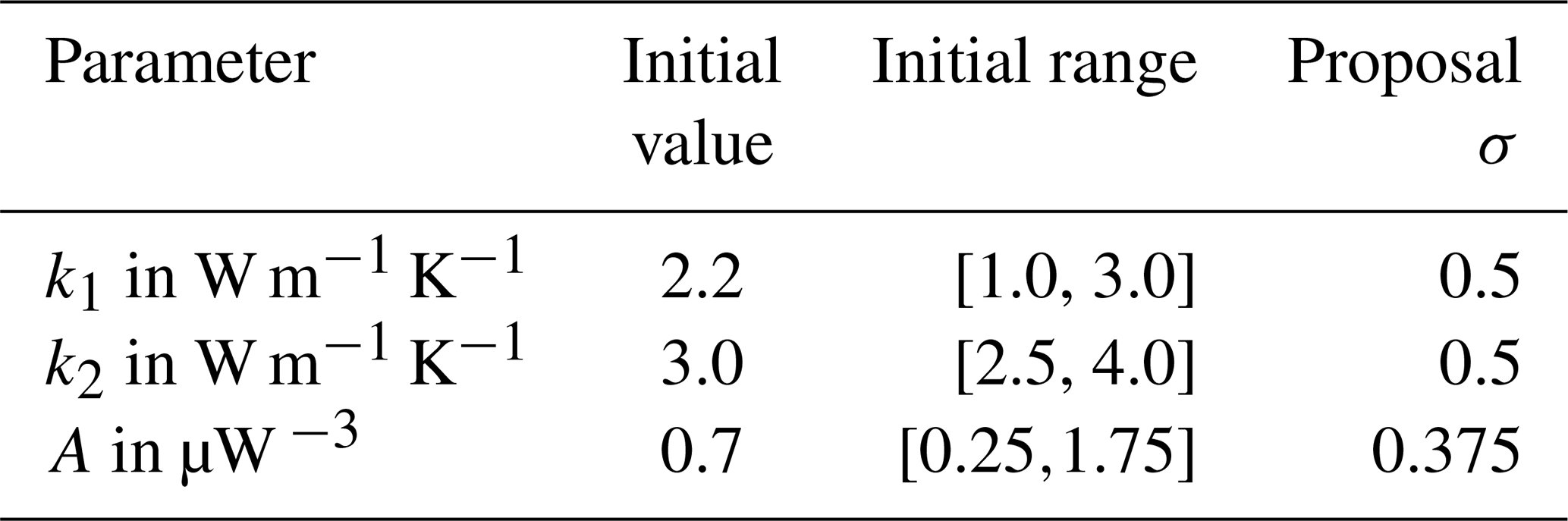
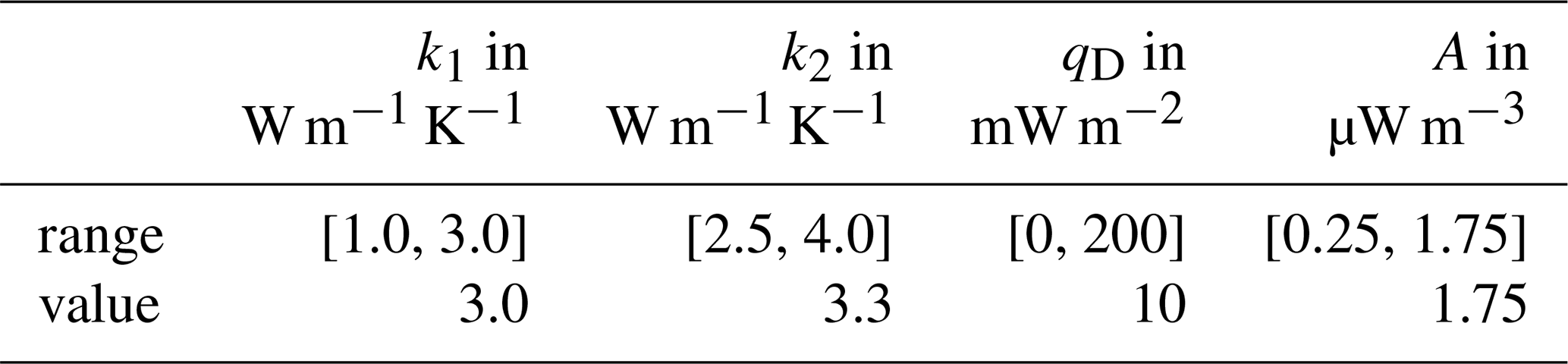
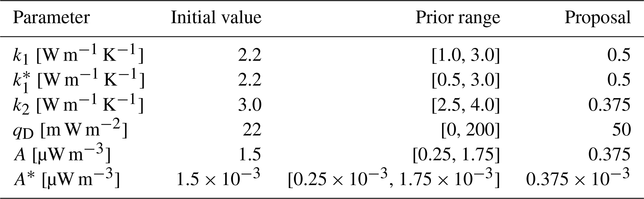
If the proposed model has a higher probability than the current model, then its parameter vector will be used as the new initial parameter vector. If the probability is lower, the proposed model can still be accepted with a probability $P_{\mathrm{new}}/P_{\mathrm{old}}>u$, where u is a uniformly distributed random number between 0 and 1. This prevents the algorithm being caught in local minima (Lösing et al., 2020). To deliver representative results, a certain number of iterations and burn-in iterations are needed. In our case, 10 000 iterations with 5000 discarded burn-in iterations are sufficient, relying on the convergence of the likelihood of the iterations as criterion. To eliminate random fluctuations, the mean of the accepted iterations gives the resulting parameter vector. We use wide uniform priors based on plausible ranges for each thermal parameter relying on previous studies (e.g., Artemieva and Mooney, 2001; Furlong and Chapman, 1987; Jaupart and Mareschal, 2014). Although higher crustal heat production up to 5 µW m⁻³ is seen for some local features, we use a more conservative value appropriate for a regional scale. The prior ranges, starting values, and proposal sizes are shown in Table 1. The proposal was tuned to achieve an acceptance ratio of 20 % to 40 %. We assume the surface temperature to be 0 °C and the LAB temperature to be 1315 °C (according to Lösing et al., 2020).

Table 1 Prior information for the inversion: initial value, range, and proposal for each iteration.

2.1 Kriging interpolation and conditional simulation

Kriging interpolation of irregularly spaced data sets provides estimates with confidence intervals (Cosentino et al., 2023). Here, we assume the mean value m₀ as given and constant, thus “simple kriging” results (Chiles and Delfiner, 1999).

$$\begin{array}{}\text{(7)}& Z^{*}=m_{\mathrm{0}}+\sum _{\mathit{\alpha }}{\mathit{\lambda }}_{\mathit{\alpha }}\left(Z_{\mathit{\alpha }}-m_{\mathit{\alpha }}\right),\end{array}$$

with the kriging estimator Z^*, the weights λ_α, the given observations Z_α, and the mean of the observations m_α. The weights are adjusted so that the resulting estimator (Eq. 7) is unbiased and the error variance minimal (Cosentino et al., 2023). A crucial parameter for kriging interpolation is the covariance function, which determines how quickly the weighting decreases with distance (Chiles and Delfiner, 1999). Here, we use the Gaussian covariance model (Webster and Oliver, 2007),

$$\begin{array}{}\text{(8)}& \mathit{\gamma }\left(r\right)={\mathit{\sigma }}^{\mathrm{2}}\left(\mathrm{1}-\exp \left[-{\left(s\cdot {\displaystyle \frac{r}{\mathrm{\ell }}}\right)}^{\mathrm{2}}\right]\right)+n,\end{array}$$

in which r represents the distance of the points, σ² the variance of the model, $s=\sqrt{\mathit{\pi }}/\mathrm{2}$ the rescaling factor, ℓ the length scale, and n the nugget.

The correlation length scale ℓ can be estimated using a semivariogram which represents the dissimilarity of pairs of points at a certain distance. Closer points tend to be more similar, increasing the distance of the points, so the dissimilarity usually also increases. The correlation length is defined as the point at which the dissimilarity reaches a certain threshold. The nugget describes small-scale effects, which is when points with very small distances have an offset to the original point (Wackernagel, 1998). A minimum number of 100 points should be used for a representative variogram for which we can define distances that resolve the resolution of the data, as well as getting an accurate estimate for the mean semivariance (Cosentino et al., 2023).

Kriging interpolation is based on a geostatistical approach, such that the interpolation result is a multivariate normal distribution. The mean (i.e., expected) value at each point is typically taken as the result and the pointwise standard deviation as uncertainty. However, this is much smoother than any realization of the actual distribution because it neglects the correlation of errors at different locations. Sparse and uneven distributed data by itself can lead to overestimation of the correlation lengths, which results in unrealistic uncertainty estimates (Chiles and Delfiner, 1999; Hadavand and Deutsch, 2020). Assuming that there is a geological region similar to the study area but with higher data coverage, we can use the covariance function (especially the correlation length) estimated for that region in the study area instead. Conditional simulation can be used to generate realizations that show possible smaller-scale variations. We use this to assess the likelihood of the NGRIP result being a local anomaly or measurement error. Conditional simulation is based on a two-stage kriging evaluation combined with an unconditional simulation. First, the given points are interpolated using the kriging method (Z^*(x)). Then a sample is drawn from the unconditional multivariate normal distribution (S(x)) based on the covariance matrix, which is in turn based on the Gaussian covariance function Eq. (8).

Finally, the unconditional sample S is conditioned upon the known data points. To do this, the difference between S(X) and the interpolated values of S(X) at the observation locations giving S^*(X) is calculated and gives the kriging variation. A conditional sample T is then obtained by

$$\begin{array}{}\text{(9)}& T\left(x\right)=Z^{*}\left(x\right)+\left(S\left(x\right)-S^{*}\left(x\right)\right).\end{array}$$

The small-scale structure of T represents possible random fluctuations, while the overall large-scale trend agrees with the kriging interpolation result (Chiles and Delfiner, 1999; Hadavand and Deutsch, 2020). The advantage of conditional simulation is the ability to overcome difficulties when dealing with sparse data to estimate non-linear and small-scale quantities (Hadavand and Deutsch, 2020).

2.2 Data

The heat flow observations analyzed in this work are located in the Arctic region north of 65° N. Observations are taken from the data sets of Lucazeau (2019) and Colgan et al. (2022). Lucazeau (2019) has introduced a global compilation of published heat flow observations. Compared to earlier compilations (e.g., Pollack et al., 1993), significant changes can be found, especially for oceanic heat flow, e.g., due to a better quality of sampling in hydrothermal regions. There are 1488 observations available for our study area. Colgan et al. (2022) compiled a database for Greenland, with 417 additional points. The analysis of the heat flow observations is mainly based on these combined 1905 points (Fig. 2).

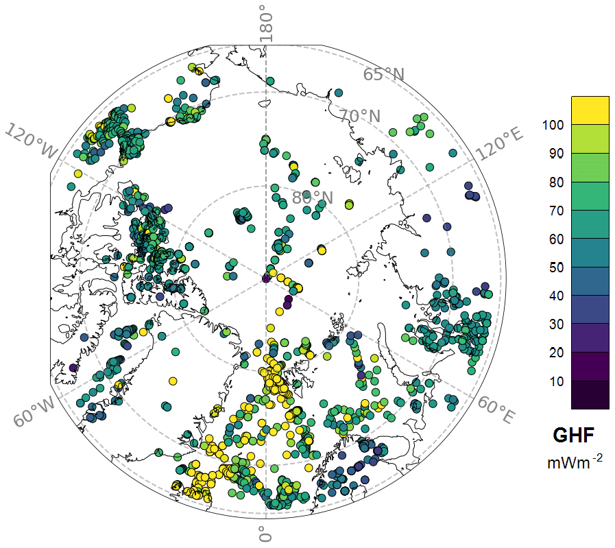
Figure 2 Heat flow for the Arctic region. Data points are from Colgan et al. (2022) and Lucazeau (2019).

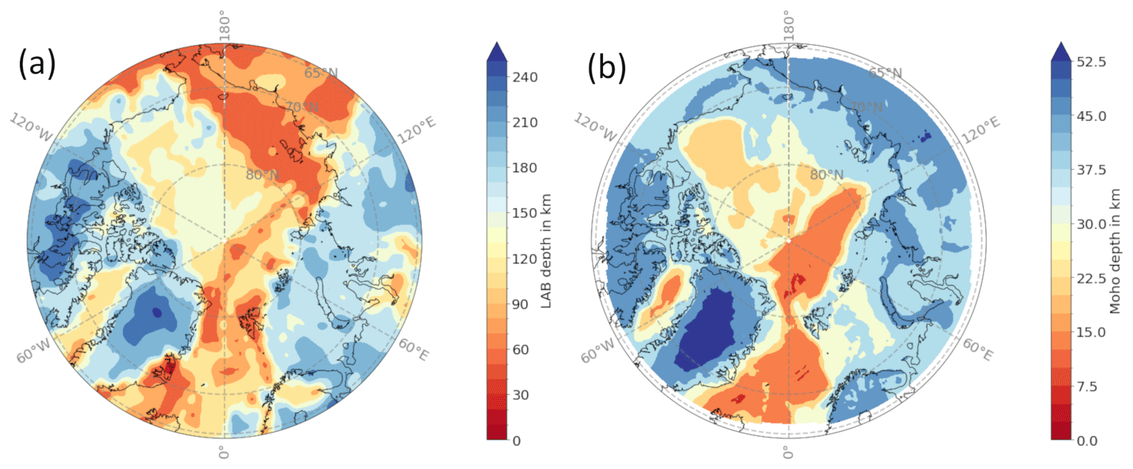
Figure 3 Input data: (a) LAB depth from the LithoRef18 (Afonso et al., 2013) and (b) Moho depth from the ArcCRUST model (Lebedeva-Ivanova et al., 2019).

In addition to the heat flow observations, we use models for the LAB depth (Afonso et al., 2019) and Moho depth (Lebedeva-Ivanova et al., 2019) for our calculations in order to make statements about the reliability to the heat flow points in relation to these solid Earth models (see Fig. 3).

The LAB depth is derived from a joint inversion of gravity anomalies, geoid height, and satellite-derived gravity gradients, and constraints from seismic, thermal, and petrological data are used (Afonso et al., 2019). For Moho depth, we use the ArcCRUST model, which is calculated from 3D-forward and 3D-inverse gravity modeling, with constraints from sediment thickness, rifting age, density, and oceanic lithosphere age (Lebedeva-Ivanova et al., 2019). These models and databases are among the most recent available for the Arctic.

For the regional analysis of continental Greenland, 47 heat flow observations are used from the Colgan et al. (2022) database which are located on Greenland or directly on the coast and extend down to 60° N.

3 Results

3.1 Agreement to solid Earth models

At each heat flow point, an ensemble of possible thermal parameter results from the MCMC approach is calculated for which we use the mean at each location as the most likely result. The correlation between the estimated thermal parameters and input parameters can be found in Appendix A.

The distribution of these mean values for the thermal parameters (Fig. 4) highlights important spatial trends and underlines where we have no fit to the LAB temperature. For most of the points in the oceanic parts, but also some points on continental lithosphere, the thermal parameters tend to strive to the upper end of the allowed parameter range, mostly coinciding with a bad fit of the LAB temperature (compare to Fig. 5). These values are unrealistically high for the thermal parameters in oceanic lithosphere, underlining the problems of applying the 1D steady-state approach to oceanic lithosphere. But this we test with the half-space cooling model. We could say that on continents that rules out the data point but requires more work on the thermal model in the oceans.

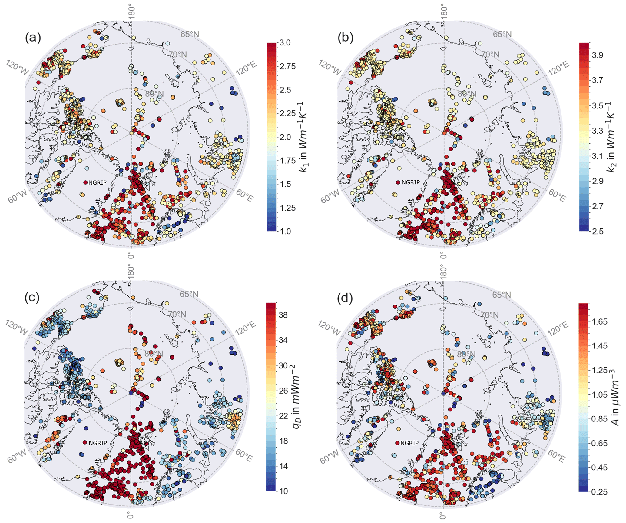
Figure 4 Distribution of the thermal parameter from the inversion with q_D calculated with Eq. (3) after 10 000 iterations per point. (a) Crustal thermal conductivity k₁, (b) mantle thermal conductivity k₂, (c) mantle heat flux q_D, and (d) crustal heat production A.

We see a trend towards the mean values of the prior parameter range for crustal (Fig. 4a) and mantle (Fig. 4b) thermal conductivity, probably indicating that they are not well resolved. This can also be seen in the distribution of the parameter correlation in Fig. A1 in the Appendix A, e.g., in relation to the Moho depth. The distribution of the crustal heat production tends to follow the GHF, with higher values at oceanic lithosphere and lower values in the continents. We also find low crustal thermal conductivity in the region of Scandinavia, which could give a hint to problematic input parameters, e.g., that the LAB in the model by Afonso et al. (2019) is too shallow (compare also to the lithospheric model by, e.g., Artemieva and Thybo, 2008). The calculated mantle heat flow follows the LAB depth and is therefore higher in oceanic lithosphere and lower in continental lithosphere. Somewhat paradoxically, the standard deviations from the MCMC runs are very small for the thermal conductivities (Appendix A) at the locations where we could not fit the temperature profile, which is caused by the result clinging to the boundary of the parameter ranges.

Our analysis shows that about two-thirds of the heat flow points can be fit with solid Earth models if adequate thermal parameters are selected (Fig. 5). However, given the range of parameters that we allow, it was impossible to achieve the desired 100 K threshold for LAB temperature at 628 locations. Most of these points are located in the oceanic lithosphere.

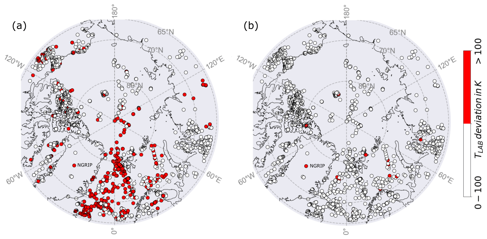
Figure 5 Deviation of the calculated compared to the pre-defined LAB temperature (a) with q_D calculated with the crustal heat production A and (b) q_D as a free parameter within the inversion. Most of the points lie within the 100 K uncertainty. For panel (a), 628 points (red) have a higher deviation, while for panel (b), the number reduces to 18 points.

Comparing Figs. 4 and 5a, we see that most of the high-parameter values occur where the LAB temperature could not be fit, so this strictly linear approach might not be appropriate to resolve oceanic lithosphere in particular. Allowing small jumps in the heat flow at the Moho leads to a non-linear representation of the temperature profile and could improve the fit of the LAB temperature for more heat flow points, e.g., where half-space cooling is assumed. We can imply this within our inversion by choosing q_D as a free parameter and estimate its value with the MCMC algorithm. To include q_D as free parameter to the inversion, we use the range based on Lösing et al. (2020), with a minimum of 0 m W m⁻², maximum of 200 m W m⁻², and a proposed standard deviation of 50 m W m⁻². With this, we reduce the number from 628 to 18 heat flow points that do not fit the solid Earth models and are able to accommodate oceanic points (Fig. 5b).

Figure 6 shows the corresponding distribution of the thermal parameters with q_D as free parameter. Mantle heat flux is highly variable, while mantle and crustal thermal conductivities and the crustal heat production tend towards the middle of the prior ranges. At points where the LAB temperature could not be fit, the crustal heat production and crustal thermal conductivity tend to have higher values and correspondingly lower standard deviations (Appendix A).

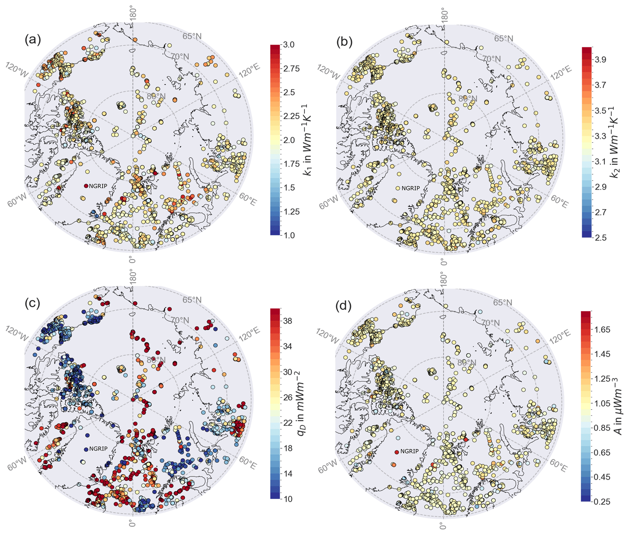
Figure 6 Distribution of the thermal parameter from the inversion with q_D as a free parameter after 10 000 iterations per point. (a) Crustal thermal conductivity k₁, (b) mantle thermal conductivity k₂, (c) mantle heat flux q_D, and (d) crustal heat production A.

To further analyze a possible limitation of our model within oceanic lithosphere, we compare a Curie depth calculated with our approaches both with and without q_D as free parameter to a Curie depth calculated with the half-space cooling model (Fig. 7). For both of our 1D approaches, we overestimate the Curie depth. We get a higher mean deviation from the half-space cooling Curie depth when q_D is not a free parameter. With q_D free, the Curie depths itself are highly scattered for younger oceanic lithosphere. For older lithosphere, our approaches underestimate the Curie depth, with a better fit for fixed q_D. Despite the deviation, we see a similar trend for the different Curie depths in oceanic lithosphere. To further evaluate oceanic lithosphere, a more advanced model like a plate model could be considered, but within our study, we may rely on the results from our simplified approach and do not necessarily need to clip oceanic lithosphere.

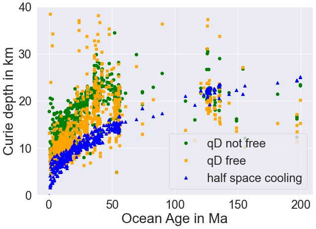
Figure 7 Comparison of the calculated associated parameter Curie depth with three different approaches within oceanic lithosphere. Blue triangles show the calculation with the half-space cooling model, while orange marks and green dots show the Curie depths calculated from the thermal parameters estimated with the 1D steady-state approach with and without q_D as a free parameter, respectively.

Comparing calculated Curie depths from our model, as described above, with the Curie depths from models with changed priors (Appendix B), we mostly get high correlations, except for about one-sixth of the points of the half-space cooling correlation. This shows that our approach seems to be robust against changes in the prior parameter ranges. The 18 remaining points are therefore especially interesting, since non-linear assumptions still do not lead to a fit. While 17 of the new low reliability points are close to other observations and can therefore be excluded without losing information on a regional scale, the NGRIP point is nearly solitary for central Greenland. Leaving it out leads either to a data gap or high uncertainties in the area of central Greenland when taking the information only from the surrounding points. However, considering this point within regional studies could be problematic, since it appears to not fit the regional geophysical models.

For NGRIP, also all parameters lie at the outer edge of the ranges (seen in Fig. 4; discrete values in Table 2), which shows that this heat flow observation of 130 m W m⁻² (Colgan et al., 2022) cannot be brought in line with the solid Earth models using these ranges and preferably should be assumed as local structure or excluded from further studies.

Table 2 Thermal parameters estimated for the NGRIP point with q_D as a free parameter within the inversion.

3.2 Kriging interpolation

Simple kriging and conditional simulation allows an investigation of the influence of isolated points in sparse regions. Due to computational costs, we limit the analysis to Greenland, but the method could also be applied to other regions. We rely on 47 heat flow observations on Greenland or directly at the coast. Within this data set, NGRIP is the only point that does not show an agreement with the regional solid Earth model.

Unfortunately, there are not enough data points in Greenland to get reliable results from the semivariogram analysis. However, if applied to the whole Arctic, the semivariogram results in a length scale of 600 km. Still, following Fox Maule et al. (2005), smaller length scales could be more reasonable. Additionally, the length scale for heat flow should be similar in geologically similar regions. Since Greenland was once part of Laurentia on the North American plate (Geoffroy et al., 2001), as well as connected to Norway (Mosar et al., 2002), we assume that a similar spatial variability occurs as in the other Precambrian shields of Scandinavia or North America (Näslund et al., 2005). Both regions are well covered with heat flow data, so a more reliable semivariogram can be estimated. With the Gaussian variogram model, we obtain a length scale for GHF of 125 km from the Scandinavian data set (Appendix C), which we then applied to Greenland (Fig. 8).

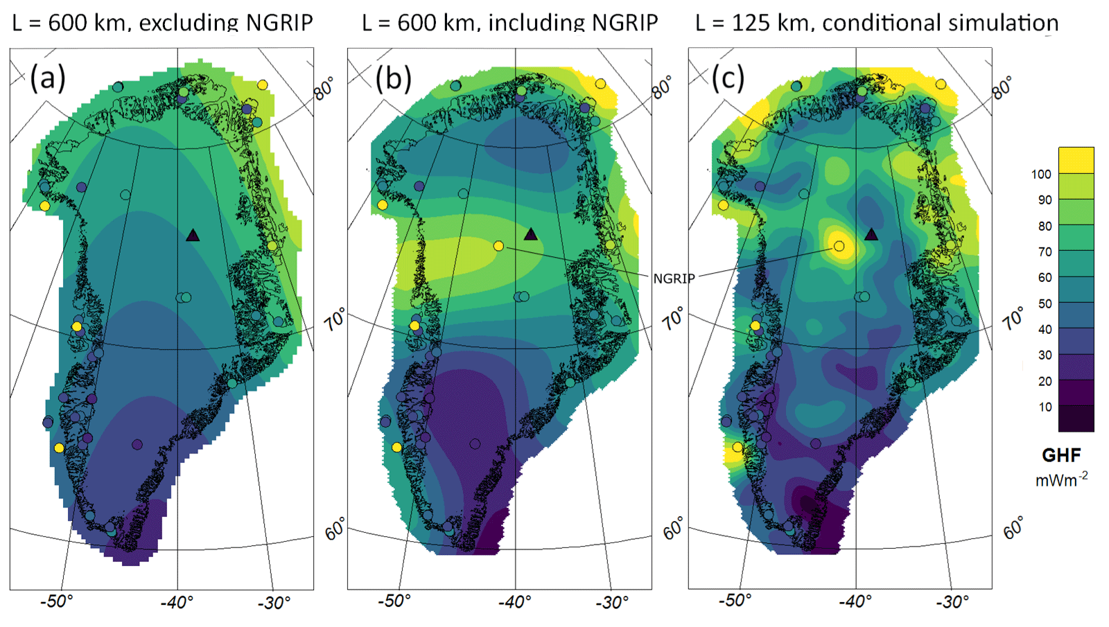
Figure 8 Kriging interpolation results for heat flow observations, (a) With a length scale of 600 km excluding the NGRIP point and (b) with a length scale of 600 km including NGRIP. (c) An example of a conditional simulation with a length scale of 125 km and NGRIP included. The triangle marks the position of the EastGRIP drill site.

Carrying out kriging interpolation, we find that, not surprisingly, NGRIP has a crucial impact on the interpolated heat flow field. Leaving it out (Fig. 8a) results in low to medium heat flow values in central Greenland, whereas, with NGRIP included (Fig. 8b), lower values are estimated in the north and significantly higher values are found in the vicinity of NGRIP, extending c. 300 km west and south. The corresponding uncertainty maps show nearly constant uncertainties of 32 m W m⁻² for Fig. 8a and 22 m W m⁻² for Fig. 8b (Appendix D). With a shorter correlation length of 125 km, and applying conditional simulation, a more realistic picture of what heat flow might look like emerges (Fig. 8c). As expected, the reduced correlation length limits the influence of the NGRIP point's high heat flow to a local area. In southern Greenland – where more points exist – GHF is comparable for all three approaches. Of course, the conditional simulation does not provide any additional constraints on the actual data (Hadavand and Deutsch, 2020).

To further judge the viability of the NGRIP point, we use conditional simulation without NGRIP as input. Simulating the unseen local structures in this way is useful if the stationary heat flow modeling (previous section) implies disagreement between regional geophysical models and the measured or inferred heat flow. Using conditional simulation, the statistical distribution of the small-scale variations can be probed to assess the possibility of a similarly extreme point occurring. We generate 100 conditional simulations of heat flow without NGRIP to investigate whether heat flow of more than 100 m W m⁻² is even possible at the NGRIP location with our assumed geostatistical parameters. An area with 500 km radius around NGRIP will be used as the “vicinity” of NGRIP.

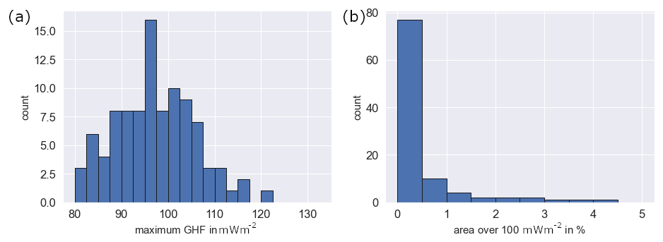
Figure 9 (a) Maximum GHF and (b) percentage of the area with a GHF over 100 m W m⁻² from 100 conditional simulations without NGRIP in the area 500 km around the NGRIP point.

In total, 38 % of the simulated heat flow fields exceed 100 m W m⁻² in the vicinity of NGRIP (Fig. 9a). A single realization reached 120 m W m⁻², but the reported value of 130 m W m⁻² is never attained. Additionally, most simulations have less than 1 % of the NGRIP area vicinity with heat flow values above 100 m W m⁻² (Fig. 9b). An area of 1 % is roughly 60 km by 60 km, so it is comparable to the length scale a single GHF hot spot in the area around NGRIP would have. However, in 13 simulations, an area of more than 1 % is covered with heat flow values higher than 100 m W m⁻², up to almost 5 % in a single simulation. Within our analysis, 60 % of the realizations have a maximum heat flow of less than 100 m W m⁻² and 87 % of the realizations have an area of less than 1 %, where 100 m W m⁻² values are reached. Thus, we can interpret this as a 40 % chance that there are any “hot spots” above 100 m W m⁻², and even if they did exist, it would be very unlikely (much less than 5 %) that NGRIP randomly “hits” the hot spot. Therefore, the high value of NGRIP cannot be explained with lateral variation at a length scale of 125 km and would be essentially incompatible with the assumed geostatistical parameters.

EastGRIP (East Greenland Ice-Core Project; triangle in Fig. 8) is a drill site in NNE Greenland with no published heat flow value so far (Rasmussen et al., 2023). This point is close to NGRIP (approximately 190 km) and could provide information on the spatial influence of NGRIP. Although its heat flow value is not yet published, we can still use the location of this point and predict interpolated values for the three different scenarios (Fig. 8). Without NGRIP, EastGRIP gets a heat flow of 61 m W m⁻². Including NGRIP increases the heat flow at EastGRIP to 81 m W m⁻² so that we see an influence of the high heat flow of NGRIP. The conditional simulation example gives the EastGRIP heat flow at 59 m W m⁻², which is significantly lower than the NGRIP value. Performing 50 conditional simulations with NGRIP, we get a variety of possible values for EastGRIP (Fig. 10).

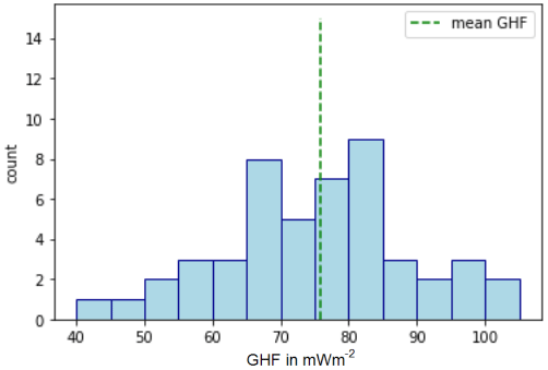
Figure 10 Heat flow values for EastGRIP extracted from 50 conditional simulations with NGRIP.

In these 50 simulations, the heat flow for EastGRIP varies from 40 to 110 m W m⁻², with a mean and median of 75 m W m⁻². Most of the simulated GHF values for EastGRIP lie within the range of 65 to 85 m W m⁻². So, we would rather assume elevated GHF at EastGRIP if the high heat flow at NGRIP is not an outlier.

3.3 Basal melt estimates

Although our models can be deemed unrealistic, we would like to briefly explore the importance for basal melt rates, following the approach from Karlsson et al. (2021) (Fig. 11). This shows the effect that local heat flow structures (Fig. 11c) might have on basal melts compared to two different regional heat flow maps (Fig. 11a and b) with an estimated geothermal basal melt for Greenland of 4.9 Gt yr⁻¹ for local structures and 5.0 Gt for regional structures.

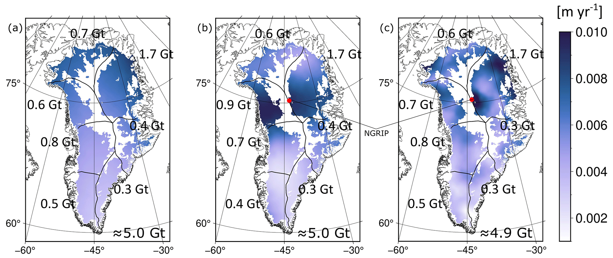
Figure 11 Basal melt estimates for Greenland based on the kriging interpolated heat flow map (a) without NGRIP and 600 km correlation length, (b) with NGRIP and 600 km correlation length, and (c) the heat flow map from the conditional simulation with 125 km correlation length and NGRIP. Blanked out areas are considered to be frozen at the ice–bedrock interface. Red point marks the location of NGRIP.

All of our maps provide similar results for the basal melt (Table 3), with insignificant variations within the single areas. It can be seen that the basal melt for a regional GHF map also shows a regional pattern following the geothermal heat, flow while we see local spots of high basal melt where we have hot spots of GHF within the local-scale map. Karlsson et al. (2021) use an average of three GHF maps (Fox Maule et al., 2009; Shapiro and Ritzwoller, 2004; Martos et al., 2018) and calculate a total geothermal basal melt of $\mathrm{5.3}+\mathrm{2.8}/-\mathrm{2.2}$ Gt. Basal melt calculated from our HF (heat flow) maps is slightly below the estimates from Karlsson et al. (2021) but would still be within their standard deviation.

Karlsson et al. (2021)

Table 3 Basal melt rates in gigatonnes per year for Greenland for four different HF maps. The different areas are the same used in Karlsson et al. (2021): NO – north, NW – northwest, NW – northeast, CW – central-west, CE – central-east, SW – southwest, SE – southeast.

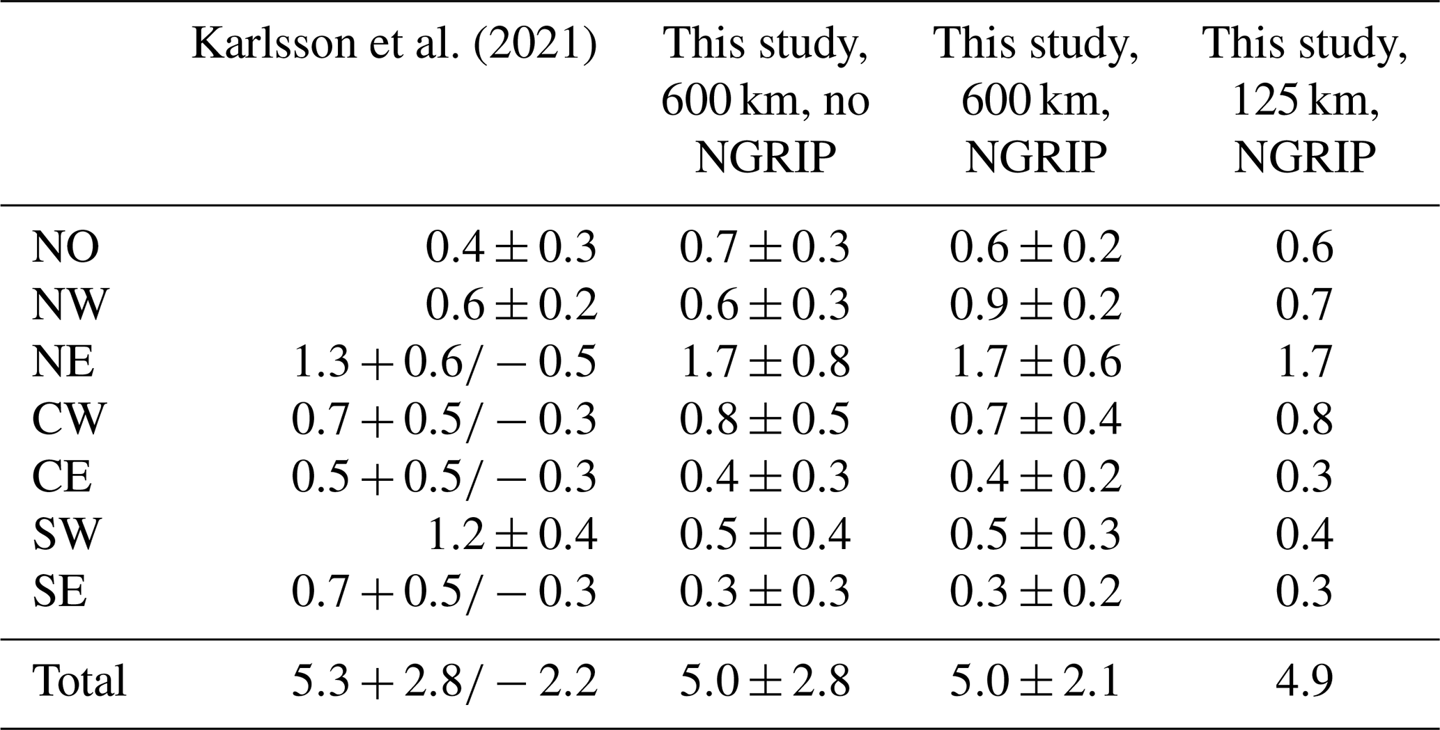
The largest contribution to basal melt from our GHF maps with 1.7 Gt comes from NE Greenland where the NGRIP point, and therefore the hot spot around NGRIP, is located. Excluding NGRIP leads to the same basal melt rate for this region. Karlsson et al. (2021) provide an estimate of $\mathrm{1.3}+\mathrm{0.6}/-\mathrm{0.5}$ Gt for this region so that our estimates are slightly higher but within the standard deviation. The major difference between our estimates and the estimate from Karlsson et al. (2021) can be found in southern Greenland, where Karlsson et al. (2021) estimate significantly more basal melt than our estimate, showing the importance of a careful assessment of heat flow data and models in order to provide accurate uncertainty estimates.

4 Discussion

We performed two analyses to appraise the spatial influence of heat flow observations. First, we used 1D stationary heat flow modeling to assess the compatibility between heat flow measurements and regional geophysical models of crustal thickness and LAB depth. Second, we focused on Greenland and relied on two related geostatistical techniques to investigate the impact of the enigmatic NGRIP point on the inferred heat flow.

We find that most of the heat flow observations in the Arctic and Greenland can be made compatible with solid Earth models, at least when allowing non-stationary heat flow at the Moho boundary. However, the stationary model fails consistently in the oceanic domain, particularly in young oceanic lithosphere. This is not surprising, since freshly formed oceanic lithosphere is cooling rapidly and far from stationary conditions.

We allow wide ranges for the geothermal parameters. Therefore, our quality criteria are fairly lenient and attention should be focused on the heat flow points that are incompatible with the geophysical models. Non-agreement could be due to four reasons: (i) our thermal model might not be adequate for this point, (ii) it could be a measurement error, (iii) the geophysical models are incorrect, or (iv) the measurement is affected by local anomalies. Thus, incompatible heat flow observations should be used with caution for regional studies, as they could represent local anomalies due to local crustal heat production (Bons et al., 2021; Hasterok and Chapman, 2011) or hydrological processes or measurement errors. In Scandinavia, incompatibility is probably due to an incorrect LAB depth, highlighting how our method can also be used to scrutinize the geophysical input models. Here, other LAB depth models (e.g., Artemieva and Thybo, 2008; Plomerová and Babuška, 2010) might improve the results, but nevertheless, such models are only available for local areas and do not cover all of our investigation area.

Deciding between the four different reasons is difficult, but the spatial distribution can be helpful. For example, in the case of the incompatible points in northern Scandinavia, there is a clear spatial correlation between incompatibility and an unusually shallow LAB depth. Likewise, any clustering of incompatible points suggests systematic issues rather than local anomalies or measurement errors. However, ultimately additional (geophysical) data will be needed to clearly determine the reason for the incompatibility.

Our second analysis is based on geostatistics. The NGRIP point is our particular focus, since it controls the interpolated heat flow over most of central Greenland, as the next heat flow observation is about 300 km away. A thorough assessment of this point is essential due to its impact on ice sheet modeling (Rogozhina et al., 2016).

We perform jackknifing for NGRIP to test its influence on the length scale of the available data that the whole of the Arctic provides. Simple kriging interpolation with poor data coverage always leads to high uncertainties (Chiles and Delfiner, 1999), which reach up to about 32 m W m⁻² when NGRIP is excluded from the interpolation data set. Additionally, performing the simple kriging interpolation with the regional length scales of 600 km confirms that excluding or including a single point can have a large influence on heat flow estimated for central Greenland.

We infer that the high GHF (above 130 m W m⁻²) measured at NGRIP is also incompatible with other heat flow estimates based on the conditional simulation. This assessment is not necessarily in disagreement with the NGRIP data because its GHF estimate is based on an extrapolated ice temperature profile since the ice–bedrock interface was not reached during drilling (Dahl-Jensen et al., 2003). An ensemble of conditional simulations shows that the high GHF (above 130 m W m⁻²) estimated at NGRIP is not compatible with other heat flow measurements in Greenland. Conditional simulations have higher variance than the pointwise standard deviation inferred by kriging interpolation because error covariances are taken into account. But even with these additional sources of variance, only about 10 % of the simulations reach values higher than 110 m W m⁻² in the vicinity of NGRIP. Provided that our geostatistical parameters (correlation and length and variance) are correct, values of GHF of more than 130 m W m⁻² are implausible and probably confined to a small region.

There are several studies of GHF in Greenland that assume large areas of elevated GHF. Martos et al. (2018) infer the GHF from the Curie depth calculated from magnetic data while assuming constant thermal conductivity (2.8 W m⁻¹ K⁻¹) and heat production (2.5 µW m⁻³). They predict an area of elevated GHF for NW–SE Greenland. After removing incompatible points, our approach estimates thermal conductivities of 2.25 W m⁻¹ K⁻¹ or lower for Greenland. The crustal heat production varies between 0.5 and 1.25 µW m⁻³. For both parameters, we estimate values that are below the assumed constant values Martos et al. (2018) use. In particular, the constant heat production they assume exceeds our range for the crustal heat production by far. Artemieva (2019) uses a thermal isostasy model based on seismic Moho depth data, topography, and the assumption that isostatic anomalies can be translated in LAB depth topography. In the region of CE Greenland, anomalously high GHF of 110 m W m⁻² is calculated that extends across Greenland. According to our analysis, such high heat flow would not influence such a large area onshore, as predicted in the model. However, the region around NGRIP shows GHF of up to 75 m W m⁻², which is compatible with our conditional simulation and interpolation results. The machine learning approach employed by Colgan et al. (2022) also suggests that the NGRIP point is incompatible with their geophysical data sets. A machine learning model without this point results in no elevated GHF for central Greenland. This is in line with the results from kriging and the conditional simulations and confirms that NGRIP should be used with caution for regional studies.

Calculating the basal melt from our GHF maps, we find that the general basal melt is similar to calculations with regional heat flow models. Our local NGRIP structure seems to punctually provide more basal melt. As stated in McCormack et al. (2022), local hot spots could have a significant influence, and not considering those structures could lead to underestimating the basal melts. When considering a local hot structure, we get similar basal melt to when choosing the same mean heat flow for Greenland without local structures. Within the single areas, the basal melt varies between the different models so that these local structures from the heat flow give local structures with high basal melts. Such local high basal melt rates could contribute to the sliding of ice shields.

Also, the area with the highest difference between the heat flow maps is found at a region not included in the calculations for basal melts, since radar data clearly show that there is no basal melt at the blanked out regions. This could be changed in future so that the contribution of these regions could be considered.

In order to verify local GHF structures, local information such as magnetic data or radar data should be included in the calculation in addition to more direct GHF observations such as the not-yet-published EastGRIP point. Furthermore, heat flow modeling could be improved by including the temperature at the top of the bedrock, as derived from ice temperature profiles in Yardim et al. (2021) and Løkkegaard et al. (2023). Using the different GHF maps in conjunction with ice temperature profiles within the 1D stationary HF equation could provide information on the reliability of the GHF maps.

With this new approach, we provide information on the reliability and locality of points and show that assuming smaller length scales is appropriate for Greenland. This approach is also applicable to the global heat flow database for evaluation of data points.

5 Conclusions

We evaluate whether the heat flow observations in the Arctic region are in agreement with regional geophysical models of LAB and Moho boundary depths using a 1D stationary heat flow model. We adjust thermal parameters (heat conductivity and radiogenic production) in a Bayesian framework, trying to reconcile geophysical LAB estimates with the heat flow data. GHF points where geophysical models and the GHF measurements disagree, are flagged, and further analyzed. The exact reason for the disagreement cannot be determined from our approach alone; it is possible that a GHF measurement only reflects local structures, e.g., due to an anomalously high crustal heat production or the disagreement could indicate errors in the GHF or geophysical models. In any case, GHF observations incompatible with regional assumptions should be used with caution for interpolations or machine learning approaches – irrespective of the reason of the disagreement. Heat flow observations are scarcely available throughout the Arctic and distributed unevenly. Due to this reason, single points are influencing large areas, creating the risk of systematic biases when used for interpolation or machine learning approaches. Conditional simulation is a geostatistical technique to incorporate local effects. While closely related to kriging interpolation, conditional simulation generates maps that include more spatial heterogeneity. This helps to investigate the occurrence of local hot spots and their spatial extent. We applied this technique to investigate whether the anomalously high GHF measurement at NGRIP is widely plausible, given the expected variability in heat flow in Greenland. Our conditional simulation results overall indicate a low probability that reported high GHF values for NGRIP are plausible. This is in line with the high uncertainty in the GHF estimate. The reliability of the GHF maps should be studied in the future in detail by replacing the constant surface temperature with observations on ice temperature profiles from radar (Yardim et al., 2021) and additional local geophysical data to obtain information on small scales.

Appendix A

The estimated mean parameters (Fig. A1; main diagonal) cover the entire range of allowed values (Table 1). Both mantle and crustal thermal conductivities show a bimodal distribution, with each having a peak at the upper boundary and the middle of their prior range. The crustal heat production is distributed nearly uniformly, again with a peak at the upper boundary. The peaks at the upper boundary of the parameter range are mostly due to points with a bad fit of the LAB temperature. Other points where the parameters also fall at the edge of the range might also be problematic, although a fit to the LAB temperature was possible. Moho and LAB depth are separated into two depths representing the continental and oceanic parts.

When looking at the correlation plots in the lower triangle, we see a high correlation between the surface heat flow q₀ and the mantle heat flow q_D. In general, there is a positive correlation from the fitted parameters to q₀ and q_D, respectively, and a slightly negative correlation between the depths and the surface heat flow and mantle heat flow.

The standard deviation of the thermal parameter estimation with the inversion is displayed in Fig. A2 for q_D (calculated) and Fig. A3 for q_D (treated as a free parameter). For both calculations, most of the points get a standard deviation from about 0.4 to 0.5 W m⁻¹ K⁻¹ for k₁ and 0.3 to 0.4 W m⁻¹ K⁻¹ for k₂. Extremely low standard deviations are mostly found where we cannot fit the temperature profiles and the parameters values themselves stick to the edges of the range. With q_D (calculated), we find low standard deviations for the crustal heat production A; when q_D is a free parameter, A gets higher standard deviations. We get highly variable standard deviations for the estimated q_D. In particular, the estimation of k₁ and k₂ seems to be quite uncertain.

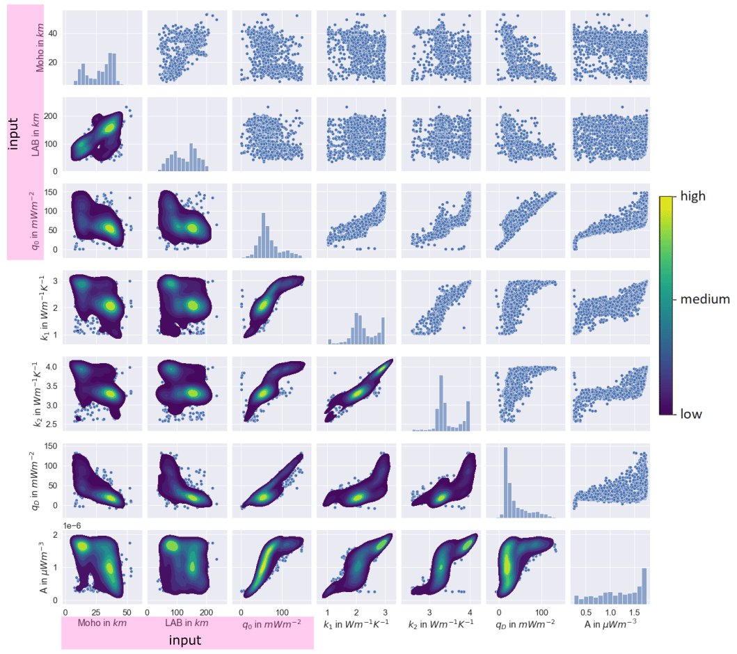
Figure A1 Correlations between the input parameters Moho and LAB depths and surface heat flow and the output parameters from the inversion crustal thermal conductivity k₁, mantle thermal conductivity k₂, mantle heat flux q_D, and crustal heat production A for all heat flow points. The upper triangle shows the inversion results as scatterplots; on the diagonal we find the histograms for each parameter. The lower triangle displays the density of the parameter combinations. Note that points with a GHF of more than 150 m W m⁻² are neglected in this figure for the purpose of clarification.

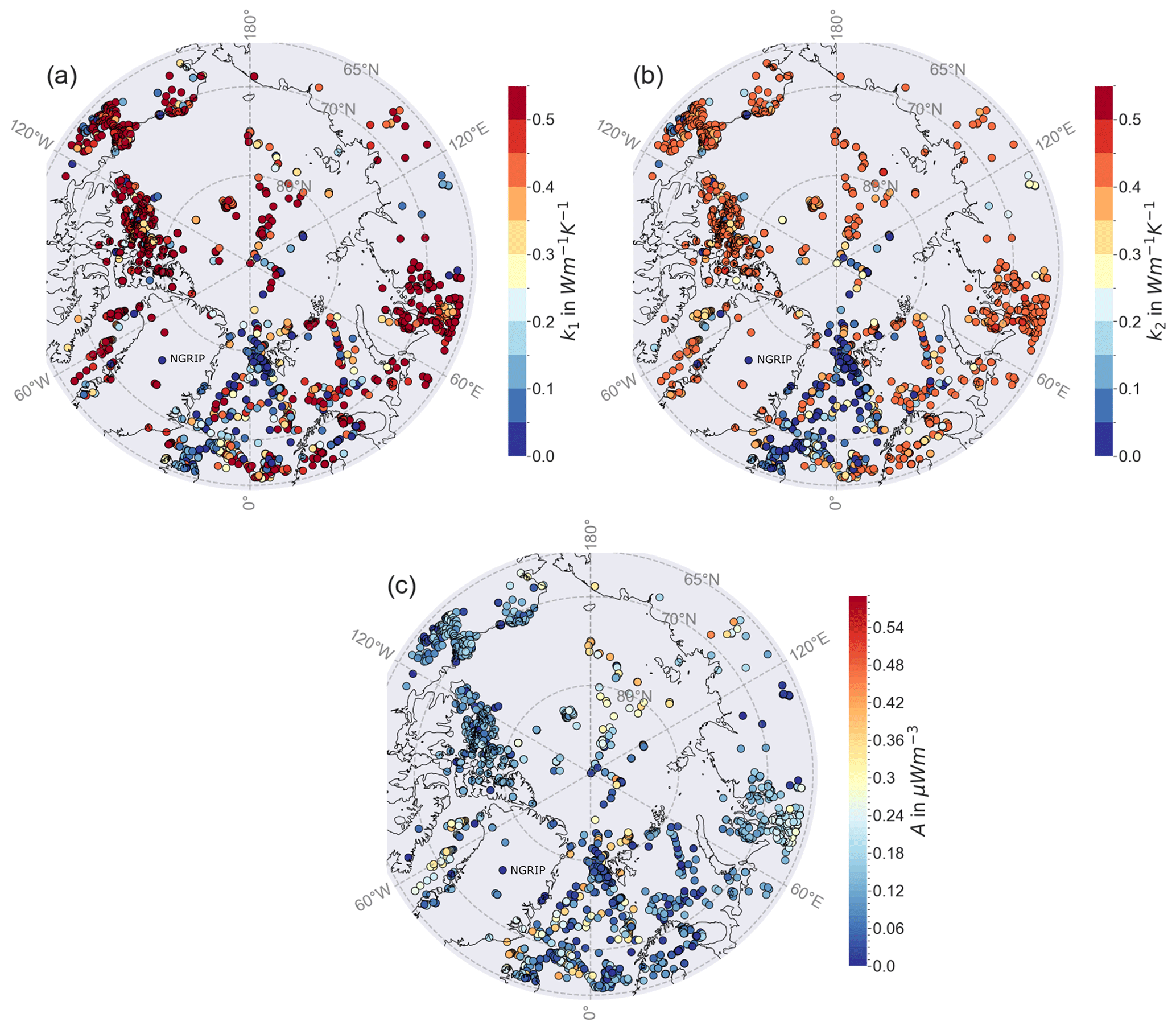
Figure A2 Distribution of the standard deviation of the thermal parameters with q_D calculated with Eq. (3). (a) Crustal thermal conductivity k₁, (b) mantle thermal conductivity k₂, and (c) crustal heat production A.

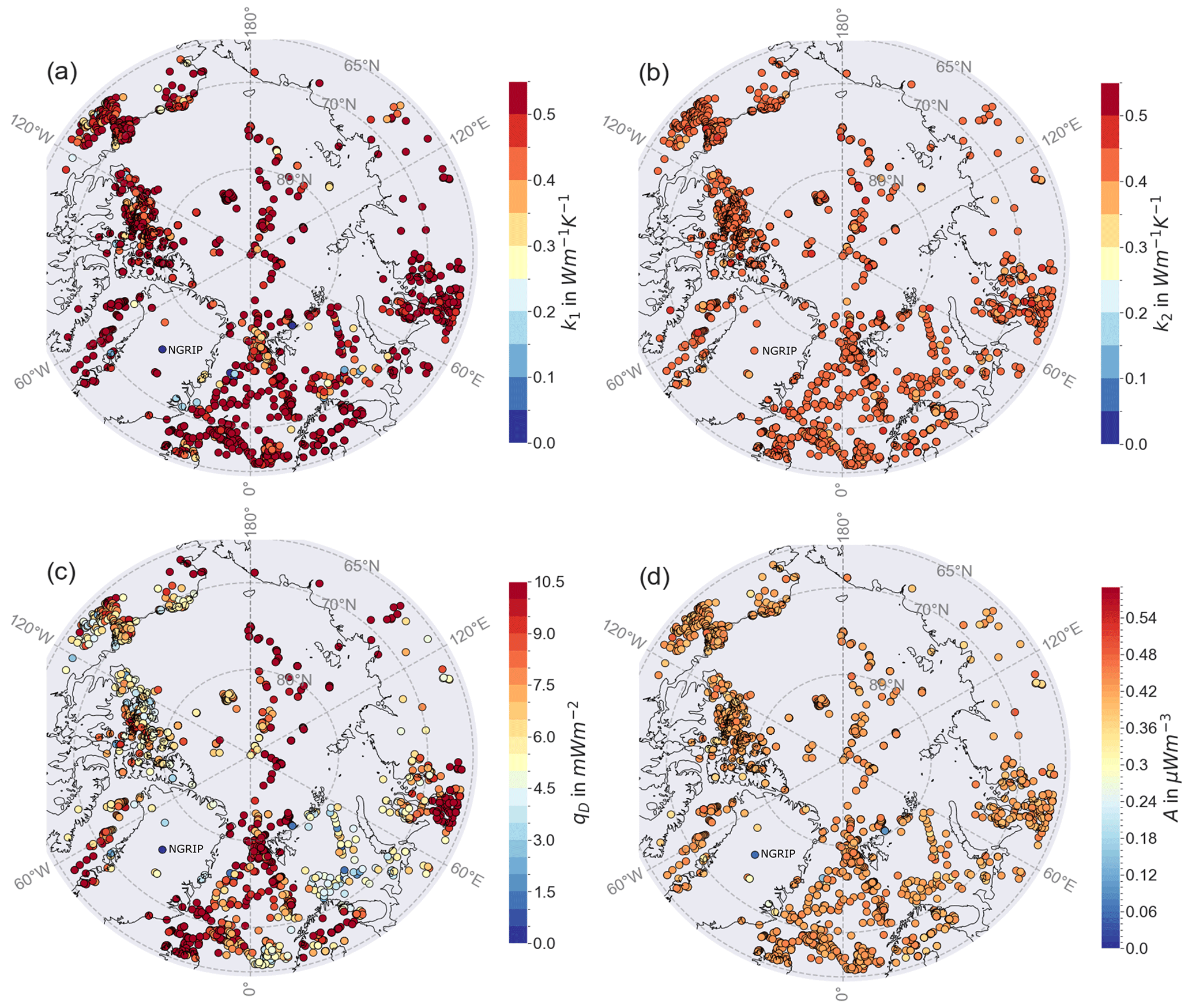
Figure A3 Distribution of the standard deviation of the thermal parameters with q_D as a free parameter. (a) Crustal thermal conductivity k₁, (b) mantle thermal conductivity k₂, (c) mantle heat flux q_D, and (d) crustal heat production A.

Appendix B

To verify that the results from our 1D stationary HF approach could basically represent an appropriate parameter distribution for whole of the area, we calculate a reference depth with different approaches. These approaches include more appropriate assumptions especially for oceanic lithosphere. The plots in Fig. B1 show the correlation between the Curie depths. We compare the reference model from the 1D stationary HF approach

$$\begin{array}{}\text{(B1)}& z_{\mathrm{Curie}}={\displaystyle \frac{\frac{q_{\mathrm{0}}}{k_{\mathrm{1}}}-\sqrt{{\left(\frac{q_{\mathrm{0}}}{k_{\mathrm{1}}}\right)}^{\mathrm{2}}-\mathrm{2}\cdot \frac{A}{k_{\mathrm{1}}}\cdot \left(T_{\mathrm{Curie}}-T_{\mathrm{0}}\right)}}{\frac{A}{k_{\mathrm{1}}}}},\end{array}$$

where T_Curie=580 °C is the temperature at the Curie depth with the Curie depth from the half-space cooling model, as well as the Curie depths from the 1D stationary HF approach, according to Eq. (B1), with variations in the prior and proposal of the thermal parameters.

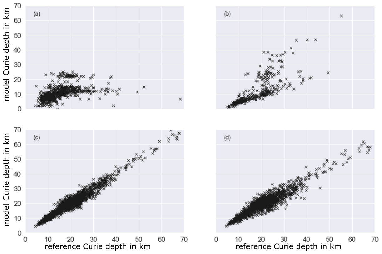
Figure B1 Correlation of different Curie depth approaches (y axis) to the reference Curie depth calculated with the 1D stationary heat flow equation with q_D estimated within the inversion (x axis). (a) Half-space cooling model (oceanic lithosphere), (b) given k₁ for Greenland points, (c) lower crustal heat production (oceanic lithosphere), and (d) combination of panel (c) with a lower crustal thermal conductivity k₁.

Table B1 Prior information for the inversion: initial value, range, and proposal for each iteration.

• a.

  For oceanic lithosphere, the assumption of purely vertical heat flow is not appropriate. We calculate the Curie depth z_Curie, based on the half-space cooling model, which is the standard approach for oceanic lithosphere

  $$\begin{array}{}\text{(B2)}& z_{\mathrm{Curie}}\left(t\right)=\mathrm{2}\sqrt{\mathit{\kappa }t}\cdot {\mathrm{erf}}^{-\mathrm{1}}\left({\displaystyle \frac{z_{\mathrm{Curie}}-T_{\mathrm{0}}}{z_{\mathrm{LAB}}-T_{\mathrm{0}}}}\right),\end{array}$$

  with the time t, temperatures T for the Curie and LAB depths, and the surface and the thermal diffusivity $\mathit{\kappa }=\mathrm{1.5}\times {\mathrm{10}}^{-\mathrm{6}}$ m² s⁻¹ (Beardsmore and Cull, 2001). Despite the different approach, we find a high correlation between the half-space cooling approach and the 1D stationary HF approach for shallow Curie depths.

• b.

  For Greenland, we change the prior of the crustal thermal conductivity to given values from the Colgan et al. (2022) database and calculate the Curie depths based on Eq. (B1). Due to a shift to lower Curie depths, we get a low correlation. Probably the shift comes from lower crustal thermal conductivities given in the database compared to the estimated ones.

• c.

  Crustal heat production can be assumed negligible for oceanic lithosphere (Beardsmore and Cull, 2001). Therefore, the prior range for heat production is set to lower values (A^* in Table B1), and the Curie depth is calculated with Eq. (B1). Changing the crustal heat production does not have a strong effect on the Curie depth.

• d.

  Last, we can adjust both the range for the crustal heat production and thermal conductivity. Based on the Colgan et al. (2022) database, the crustal thermal conductivity could be lower than initially assumed. The used values A^* and $k_{\mathrm{1}}^{*}$ are displayed in Table B1. Combining this with the assumption of lower crustal heat production within the oceanic crust, we calculate the Curie depths (Eq. B1). We get a good correlation but a higher deviation for the Curie depths compared to approach (c).

Based on the correlation of the Curie depths, we can assume that our initial approach is appropriate for the analysis, since it is robust to changes in the parameter space. Even for the comparison for the oceanic crust, we find somewhat high correlations between the different approaches for shallow Curie depths.

Appendix C

Due to the geological similarity, we take the length scales calculated from the semivariogram for the heat flow in Scandinavia (Lucazeau, 2019). Here, we have a high data coverage so that estimates based on the semivariogram are appropriate (Fig. C1). For Scandinavia, we calculate a length scale of 125 km.

Comparing the semivariograms (Fig. C2), we see that for Scandinavia we get a lot of points, especially on short distances, so that the Gaussian variogram model can easily be fitted. For the semivariogram of Greenland, we see that we generally get fewer points to fit. A fit with the Gaussian variogram model is possible, but there are large outliers up to a distance of 500 km, so that it is less appropriate to rely on this semivariogram for length-scale estimates.

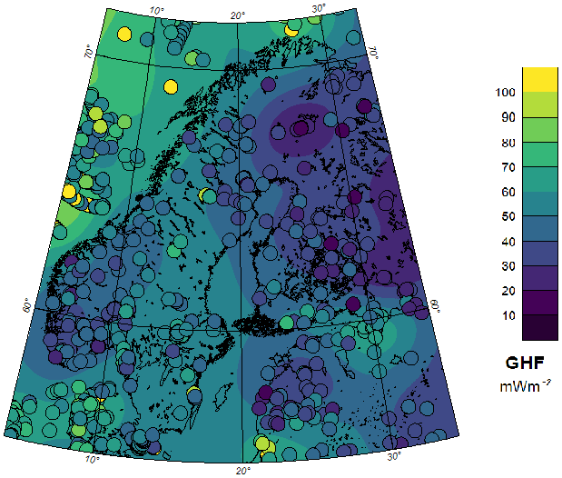
Figure C1 Kriging interpolation of the heat flow and observation distribution in Scandinavia.

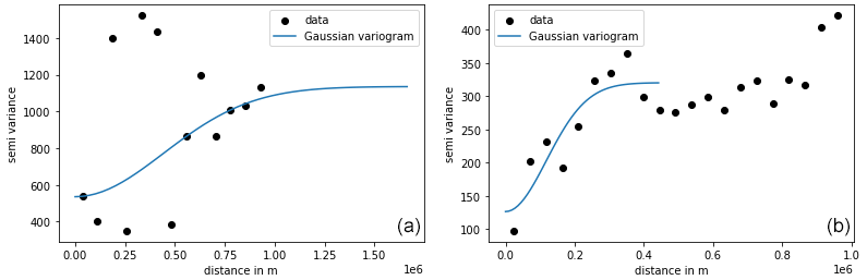
Figure C2 Semivariogram for the given heat flow observations for (a) Greenland and (b) Scandinavia.

Appendix D

Kriging provides the uncertainties for our interpolated heat flow map. For both regional heat flow maps, the uncertainty maps are shown in Fig. D1. While excluding NGRIP (right) shows uncertainties between 29 and 35 m W m⁻², including NGRIP (left) leads to lower uncertainties of 20 to 25 m W m⁻², with higher uncertainties at northeast Greenland. Within both maps, we get edge effects.

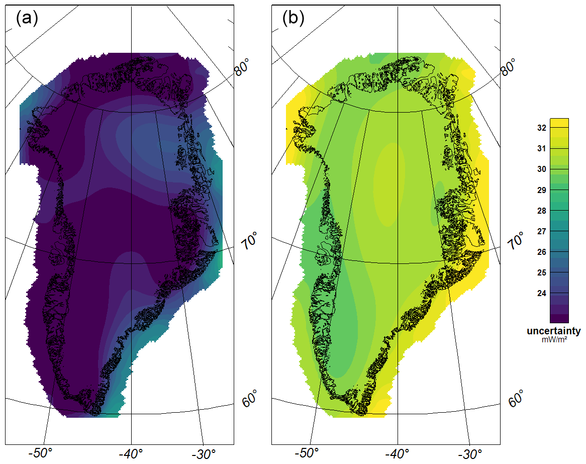
Figure D1 Uncertainty maps of the kriging interpolation (a) with and (b) without NGRIP.