Seismic wave modeling of fluid-saturated fractured porous rock: including fluid pressure diffusion effects of discretely distributed large-scale fractures

The scattered seismic waves of fractured porous rock are strongly affected by the wave-induced fluid pressure diffusion effects between the compliant fractures and the stiffer embedding background. To include these poroelastic effects in seismic modeling, we develop a numerical scheme for discretely distributed large-scale fractures embedded in fluid-saturated porous rock. Using Coates and Schoenberg's local-effective-medium theory and Barbosa's dynamic linear slip model characterized by complex-valued and frequency-dependent fracture compliances, we derive the effective viscoelastic compliances in each spatial discretized cell by superimposing the compliances of the background and the fractures. The effective governing equations for fractured porous rocks are viscoelastic anisotropic and numerically solved by the mixed-grid-stencil frequency-domain finite-difference method. The main advantage of our proposed modeling scheme over poroelastic modeling schemes is that the fractured domain can be modeled using a viscoelastic solid, while the rest of the domain can be modeled using an elastic solid. We have tested the modeling scheme in a single fracture model, a fractured model, and a modified Marmousi model. The good consistency between the scattered waves off a single horizontal fracture calculated using our proposed scheme and the poroelastic modeling validates that our modeling scheme can properly capture the fluid pressure diffusion (FPD) effects. In the case of a set of aligned fractures, the scattered waves from the top and bottom of the fractured reservoir are strongly influenced by the FPD effects, and the reflected waves from the underlying formation can retain the relevant attenuation and dispersion information. The proposed numerical modeling scheme can also be used to improve migration quality and the estimation of fracture mechanical characteristics in inversion.

1 Introduction

Fluid-saturated porous rocks in a reservoir, which are characterized by a heterogeneous internal structure consisting of a solid skeleton and interconnected fluid-filled voids, are often permeated by much more compliant and permeable fractures. Although the fractures typically occupy only a small volume, they tend to dominate the overall mechanical and hydraulic properties of the reservoir (Liu et al., 2000; Gale et al., 2014). Thus, fracture detection, characterization, and imaging are of great importance for hydrocarbon exploration and production. Seismic waves are widely used for these purposes because their amplitude, phase, and anisotropy properties can be strongly affected by the fractures (Chapman, 2003; Gurevich, 2003; Brajanovski et al., 2005; Rubino et al., 2014). Therefore, appropriate numerical modeling methods are required for the interpretation, migration, and inversion of seismic data from porous media containing discretely distributed fractures.

Biot's poroelastic theory (Biot, 1956a, b) is the fundamental theory to describe elastic wave propagation in fluid porous media, including the dynamic interactions between rock and pore fluid. However, the original theory, assuming a macroscopically homogeneous porous media saturated by a single fluid phase, fails to explain the measured velocity dispersion and attenuation of seismic waves (Nakagawa and Schoenberg, 2007). In recent decades, many researchers have found that if porous media contains mesoscale heterogeneity, a local fluid pressure gradient will be induced at a scale comparable to the fluid pressure diffusion length at the seismic frequency band, thus causing significant velocity dispersion and attenuation (White et al., 1975; Dutta and Odé, 1979a, b; Johnson, 2001; Müller et al., 2008; Norris, 1993; Gelinsky and Shapiro, 1997; Kudarova et al., 2016). Fractures embedded in homogeneous porous background are special heterogeneities, exhibiting strong mechanical contrasts with background. When seismic waves travel through fluid-saturated fractured porous rocks, local fluid pressure gradients will be induced between the fractures and the background in response to the strong compressibility contrast. To return the equilibrium state, fluid pressure diffusion (FPD) occurs between the fractures and the embedding background, which in turn changes the fluid stiffening effect on the fractures and thus their mechanical compliances depending on frequency (Barbosa et al., 2016a, b).

When the fractures with spacing and length much smaller than the wavelengths are uniformly and regularly distributed, the properties of the fractured rocks are homogeneous at macroscopic scale and can be described by a representative elementary volume (REV). Various effective medium theories are available for estimating the fracture-induced anisotropy, attenuation, and dispersion in a poroelastic context (Hudson, 1981; Thomsen, 1995; Chapman, 2003; Brajanovski et al., 2005; Krzikalla and Müller, 2011; Galvin and Gurevich, 2015; Guo et al., 2017a, b). However, large-scale fractures with much larger spacing and length typically have a more complex discrete distribution rather than a regular one; therefore, the properties of rocks containing such fractures cannot be modeled by the effective medium theory. In contrast, the linear slip model (LSM) (Schoenberg, 1980), which represents individual fractures as nonwelded interfaces with discontinuous displacement tensors, is not limited by the assumption of regular distribution and can be used to model the discretely distributed fractures. Due to the discrete distribution, the effects of large-scale fractures are not uniform and vary spatially, which means that their effects cannot be represented by a single REV. In the framework of LSM, two numerical schemes are available to assess the seismic response of discretely distributed large-scale fractures: the local-effective-medium schemes (Coates and Schoenberg, 1995; Oelke et al., 2013) and the explicit-interface scheme (Zhang, 2005; Cui et al., 2018; Khokhlov et al., 2021). The local-effective-medium scheme uses a very coarse mesh to discretize background media and incorporates the additional effects of fractures within each discretized cell based on LSM; that is, it regards each discretized cell as a REV. The advantage is that it requires no special treatment of the displacement discontinuity conditions on the fractures, which means no additional memory and computation costs. The explicit-interface scheme uses a very fine mesh to discretize fractures and directly treats the displacement discontinuity across each fracture without any equivalent treatment, resulting expensive memory and computation costs.

The common aspect of the aforementioned numerical modeling schemes is that they are all implemented in a purely elastic LSM with real-valued compliance boundaries and represent both the embedding background and fractures as elastic solids; thus, the impact of FPD effects on seismic scattering cannot be accounted for. A dynamic linear slip model incorporating FPD effects should be considered when implementing numerical modeling of seismic waves propagating in fluid-saturated porous rocks containing discretely distributed large-scale fractures. Nakagawa and Schoenberg (2007) developed an extended poroelastic LSM (PLSM) for a single fracture. The proposed model representing both the background and the fracture as poroelastic media can appropriately incorporate the frequency-related effects, but it will also result in a higher computational consumption and more memory requirements. Rubino et al. (2015) proposed a frequency-dependent complex-valued normal compliance for a set of aligned fractures with a separation much smaller than the prevailing seismic wavelength. Despite the ability of including the FPD across the fractures, the model is not suitable for modeling discretely distributed fractures. In the context of viscoelasticity, Barbosa et al. (2016a) developed a viscoelastic linear slip model (VLSM) for an individual fracture with explicit complex-valued and frequency-dependent fracture compliances to account for the impact of FPD on the fracture stiffness. That provides a viscoelasticity-based modeling algorithm for discretely distributed large-scale fractures with smaller computational costs and memory requirements than the poroelasticity-based modeling.

In this paper, we develop a viscoelastic numerical modeling scheme to simulate seismic wave propagation in fluid-saturated porous media containing discretely distributed large-scale fractures. To capture the FPD effects between the fractures and background, we use the local-effective-medium theory based on Barbosa's VLSM to derive the effective anisotropic viscoelastic compliances in each numerical cell by superimposing the compliances of the background and the fractures. The effective anisotropic viscoelastic governing equations of the fractured porous rock are then numerically solved using the mixed-grid-stencil frequency-domain finite-difference method (FDFD) (Hustedt et al., 2004; Operto et al., 2009; Liu et al., 2018). Compared to poroelastic modeling scheme, the main advantage of our modeling scheme is that it uses VLSM-based viscoelastic modeling to account for FPD effects in the domain permeated by fractures, while in the rest fracture-free domain, it uses elastic modeling. To validate that the proposed viscoelastic modeling scheme can capture the impact of FPD effects on seismic wave scattering, we compare the scattered waves of a single horizontal fracture obtained using our proposed modeling scheme with the poroelastic modeling scheme and elastic modeling scheme. Numerical examples of a fractured reservoir are presented to demonstrate that the proposed modeling scheme can properly simulate the wave attenuation and dispersion due to the FPD effects between the fracture system and background. A set of rock physics models were generated by the Marmousi model to test the proposed modeling scheme and code. The scheme can be used not only to study the impact of mechanical and hydraulic of fracture properties on seismic scattering but can also to improve migration quality and the estimation of fracture mechanical characteristics in inversion.

2 Review of the LSM

The LSM was originally proposed by Schoenberg (1980) to represent a solid- or fluid-infilled fracture permeated in a pure solid background, and then it was extended by other researchers (e.g., Nakagawa, Barbosa) to represent a poroelastic fracture to include the FPD effects. We briefly review the original LSM and its poroelastic and viscoelastic extensions.

2.1 The original LSM

Schoenberg (1980) presented the original LSM in the context of elasticity, representing both the background and the fracture as elastic solids. The original LSM assumes that across a fracture surface the stresses are continuous while the displacements are discontinuous. The discontinuous displacement vector of a horizontal fracture is linearly related to the stress tensor through the fracture compliance, which can be written as

$$\begin{array}{}\text{(1)}& \begin{array}{rl}& \left[u_x\right]=Z_{\mathrm{T}}{\mathit{\sigma }}_{xz},\\ & \left[u_y\right]=Z_{\mathrm{T}}{\mathit{\sigma }}_{yz},\\ & \left[u_z\right]=Z_{\mathrm{N}}{\mathit{\sigma }}_{zz},\end{array}\end{array}$$

where [u_i] represents the discontinuous displacement components, σ_ij represents the stress components, and $Z_{\mathrm{N}}=h/H$ and $Z_{\mathrm{T}}=h/\mathit{\mu }$ are the normal and tangential compliance of the fracture, respectively. H and μ are the P-wave and shear modulus of the fracture, and h is the thickness of the fracture. Due to the simple expression, the original LSM can be easily incorporated into the local-effective-medium theory to model seismic wave scattering off large-scale fractures. However, the original LSM was derived in a purely elastic context, only suitable for fractures filled with pure solids or fluids; thus, it is not competent to describe the FPD effects.

2.2 Nakagawa's PLSM

Nakagawa and Schoenberg (2007) presented a PLSM in the framework of poroelasticity, representing the fracture as a highly compliant and porous thin isotropic, homogeneous layer embedded in a much stiffer and much less porous background (Nakagawa et al., 2007; Barbosa et al., 2016a). Similar to the classic LSM, the PLSM assumes that across a fracture surface the stresses are continuous while the displacements are discontinuous. The discontinuous displacement components for a horizontal fracture are (Nakagawa and Schoenberg, 2007)

$$\begin{array}{}\text{(2)}& \begin{array}{rl}& \left[u_x\right]=Z_{\mathrm{T}}{\mathit{\sigma }}_{xz},\\ & \left[u_y\right]=Z_{\mathrm{T}}{\mathit{\sigma }}_{yz},\\ & \left[u_z\right]=Z_{{\mathrm{N}}_{\mathrm{D}}}\left({\mathit{\sigma }}_{zz}+\mathit{\alpha }{P}_{\mathrm{f}}\right),\\ & \left[w_z\right]=-\mathit{\alpha }{Z}_{{\mathrm{N}}_{\mathrm{D}}}\left({\mathit{\sigma }}_{zz}+{\displaystyle \frac{\mathrm{1}}{B}}{P}_{\mathrm{f}}\right),\end{array}\end{array}$$

where $Z_{{\mathrm{N}}_{\mathrm{D}}}=h/H_{\mathrm{D}}$ and $Z_{\mathrm{T}}=h/\mathit{\mu }$ are the fracture's drained normal compliance and tangential compliance, respectively; H_D and H_U are the fracture's drained and undrained P-wave modulus, respectively; α is Biot's effective stress coefficient of the fracture; and $B=\mathit{\alpha }M/H_{\mathrm{U}}$ is the fracture's uniaxial Skempton coefficient. Since the PLSM represents both the background and the fracture as poroelasticity, it is capable of describing the discontinuous displacement of the relative fluid in addition to the solid, implying that it can properly handle the FPD effects between the background and the fracture. Although it is difficult to incorporate the PLSM into the effective medium theory to obtain the effective moduli of the fractured porous rock, these boundary conditions can be easily incorporated into the poroelastic finite-difference algorithm for modeling seismic wave scattering off large-scale fractures parallel to the coordinate axis. An alternative wavenumber domain method for modeling the scattered waves by poroelastic fractures is presented by Nakagawa and Schoenberg (2007) based on the PLSM.

2.3 Barbosa's VLSM

Barbosa et al. (2016a) derived a VLSM that accounts for the FPD effects between a fracture and background and the resulting stiffening effect impact on the fracture. The background is assumed to be not impacted by the FPD and can be represented by an elastic solid, whose properties are computed according to Gassmann's equation (Gassmann, 1951). By representing fractures as extremely thin viscoelastic layers, the poroelastic effects were incorporated into the classical LSM through complex-valued and frequency-dependent compliances. These compliances characterize the mechanical properties of the fluid-saturated fracture.

The discontinuous displacement components of the VLSM (Barbosa et al., 2016a) for a horizontal fracture are

$$\begin{array}{}\text{(3)}& \begin{array}{rl}& \left[u_x\right]=Z_{\mathrm{T}}{\mathit{\sigma }}_{xz},\\ & \left[u_y\right]=Z_{\mathrm{T}}{\mathit{\sigma }}_{yz},\\ & \left[u_z\right]=Z_{\mathrm{N}}{\mathit{\sigma }}_{zz}+Z_X{\mathit{\epsilon }}_{xx},\end{array}\end{array}$$

where Z_N and Z_T are generalized normal and tangential compliances of the fracture, respectively, and Z_X is a parameter that relates to the coupling between horizontal and vertical deformation of the fracture. The normal compliance Z_N and additional parameter Z_X are complex-valued and frequency-dependent, while the tangential compliance $Z_{\mathrm{T}}=h/\mathit{\mu }$ is the same as for elastic and poroelastic models. The two frequency-dependent and complex-valued compliances are

$$\begin{array}{}\text{(4)}& \begin{array}{rl}& Z_{\mathrm{N}}=Z_{{\mathrm{N}}_{\mathrm{U}}}+Z_{{\mathrm{N}}_{\mathrm{D}}}{\displaystyle \frac{G_{\mathrm{1}}\left(\mathrm{1}+i\right)}{\sqrt{\mathit{\omega }}+G_{\mathrm{2}}\left(\mathrm{1}+i\right)}},\\ & Z_X=-{\displaystyle \frac{G_{\mathrm{3}}\left(\mathrm{1}+i\right)}{\sqrt{\mathit{\omega }}+G_{\mathrm{4}}\left(\mathrm{1}+i\right)}},\end{array}\end{array}$$

where $Z_{{\mathrm{N}}_{\mathrm{U}}}=h/H_{\mathrm{U}}$ and $Z_{{\mathrm{N}}_{\mathrm{D}}}=h/H_{\mathrm{D}}$ are the fracture's undrained and drained normal compliance, respectively, and ω is the angular frequency. The four real-valued parameters G₁, G₂, G₃, and G₄ are defined as

$$\begin{array}{}\text{(5)}& \begin{array}{rl}& G_{\mathrm{1}}={\displaystyle \frac{{\mathit{\kappa }}^{\mathrm{b}}}{\mathit{\eta }{Z}_{{\mathrm{N}}_{\mathrm{D}}}}}{\displaystyle \frac{{\left(B^{\mathrm{b}}-B^{\mathrm{f}}\right)}^{\mathrm{2}}}{\sqrt{D^{\mathrm{b}}}}},G_{\mathrm{2}}={\displaystyle \frac{{\mathit{\kappa }}^{\mathrm{b}}}{\mathit{\eta }{Z}_{{\mathrm{N}}_{\mathrm{D}}}}}{\displaystyle \frac{B^{\mathrm{f}}}{{\mathit{\alpha }}^{\mathrm{f}}\sqrt{D^{\mathrm{b}}}}},\\ & G_{\mathrm{3}}={\displaystyle \frac{\mathrm{2}\sqrt{\mathrm{2}}{\mathit{\alpha }}^{\mathrm{b}}{\mathit{\mu }}^{\mathrm{b}}\left(B^{\mathrm{f}}-B^{\mathrm{b}}\right)\sqrt{D^{\mathrm{b}}}}{H_{\mathrm{D}}^{\mathrm{b}}}},\\ & G_{\mathrm{4}}={\displaystyle \frac{\sqrt{\mathrm{2}}{\mathit{\kappa }}^{\mathrm{b}}{D}^{\mathrm{f}}}{Z_{\mathrm{T}}{\mathit{\mu }}^{\mathrm{f}}{\mathit{\kappa }}^{\mathrm{f}}\sqrt{D^{\mathrm{b}}}}},\end{array}\end{array}$$

where κ is the permeability, η is the viscosity of the fluid, $D=\frac{\mathit{\kappa }}{\mathit{\eta }}\frac{H_{\mathrm{D}}M}{H_{\mathrm{U}}}$ is the diffusivity, and the other parameters are defined in the same way as in poroelasticity. The parameters in Eq. (5) with superscripts b correspond to background properties, and the parameters with superscripts f correspond to fracture parameters.

In the low-frequency limit, the two frequency-dependent and complex-valued parameters become

$$\begin{array}{}\text{(6)}& \begin{array}{rl}& Z_{\mathrm{N}}=Z_{{\mathrm{N}}_{\mathrm{U}}}+Z_{{\mathrm{N}}_{\mathrm{D}}}{\displaystyle \frac{G_{\mathrm{1}}}{G_{\mathrm{2}}}},\\ & Z_X=-{\displaystyle \frac{G_{\mathrm{3}}}{G_{\mathrm{4}}}}.\end{array}\end{array}$$

The frequency-independent and real-valued parameters in Eq. (6) indicate the elastic behavior of the fracture, which is expected, since the fluid pressure between the fracture and background at low frequencies has enough time to equilibrate within a half-wave period (i.e., the fracture is softest), resulting in no dispersion and attenuation of the seismic waves.

In the high-frequency limit, the two frequency-dependent and complex-valued parameters become

$$\begin{array}{}\text{(7)}& \begin{array}{rl}& Z_{\mathrm{N}}=Z_{{\mathrm{N}}_{\mathrm{U}}},\\ & Z_X=\mathrm{0}.\end{array}\end{array}$$

Equation (7) indicates that the fracture model collapses to an elastic thin layer model in the high-frequency limit, which is consistent with the original LSM that computes the properties of both the fracture and background using Gassmann's equations. This because at high frequencies the fluid pressure between the fracture and background has no time to equilibrate within a half-wave period; i.e., the fracture is hardest and behaves as being sealed. The VLSM considering FPD effects can be incorporated into the local-effective-medium theory to simulate the poroelastic seismic response of large-scale fractures, while its low- and high-frequency limits can be used to model the elastic seismic response.

According to Barbosa et al. (2016a), there are two distinct frequency regimes due to the FPD effect, and the characteristic frequency for the transition between the two regimes is

$$\begin{array}{}\text{(8)}& {\mathit{\omega }}_m=\mathrm{2}\mathit{\pi }{f}_m={\left({\displaystyle \frac{\mathrm{2}}{h}}\right)}^{\mathrm{2}}\left({\displaystyle \frac{e_{\mathrm{b}}^{\mathrm{2}}}{e_{\mathrm{f}}^{\mathrm{2}}+e_{\mathrm{f}}{e}_{\mathrm{b}}}}\right)D_{\mathrm{f}},\end{array}$$

where h is the thickness of the fracture, D is the diffusivity, $e=\mathit{\kappa }/\mathit{\eta }\sqrt{D}$, and the subscripts b and f correspond to background fracture parameters, respectively.

3 Seismic modeling of fractured porous rock

In this section, we focus on the implementation of seismic modeling of fluid-saturated porous media containing discretely distributed large-scale fractures in the 2-D case. We develop a viscoelastic modeling scheme based on the VLSM and local-effective-medium theory (Coates and Schoenberg, 1995) to incorporate the FPD effects between fractures and background. To validate that the proposed viscoelastic modeling scheme can capture the impact of FPD effects on seismic wave scattering of fractures, we outline the implementation of the poroelastic modeling scheme using an explicit application of the PLSM.

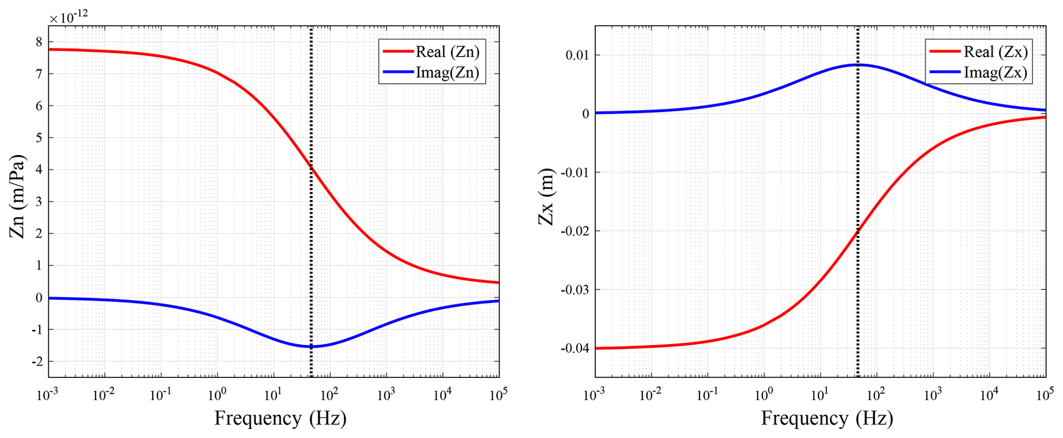
Figure 1 Complex-valued and frequency-dependent Z_N and Z_X. The dashed vertical line denotes the characteristic frequency computed using Eq. (8).

3.1 Viscoelastic modeling based on VLSM

To incorporate the VLSM into viscoelastic finite-difference modeling algorithms, we adopt Coates and Schoenberg's local-effective-medium theory (1995) to account for the property of each fracture. We first provide the specific derivation of the effective viscoelastic–anisotropic stiffness matrix of the numerical cell by superimposing the compliances of the background and the fractures. The porous background is assumed to be unaffected by the FPD in the presence of fractures because of the small amount of diffusing fluid and large compliance contrast between background and fluid. Thus, the rock background can be represented by an elastic homogeneous solid, and its strain tensor ε^b can be expressed as

$$\begin{array}{}\text{(9)}& {\mathit{\epsilon }}_{ij}^{\mathrm{b}}=s_{ijkl}^{\mathrm{b}}{\mathit{\sigma }}_{kl},\left(i,j=x,y,z\right),\end{array}$$

where the compliance tensor s^b is computed according to Gassmann's equation (Rubino et al., 2015), and σ is the average stress tensor. The exceeded strain tensor ε^c induced by a single fracture with surface S in a representative volume V (e.g., the volume of numerical cell) is given by (Sayers and Kachanov, 1995; Liu et al., 2000)

$$\begin{array}{}\text{(10)}& {\mathit{\epsilon }}_{ij}^c=s_{ijkl}^c{\mathit{\sigma }}_{kl}={\displaystyle \frac{\mathrm{1}}{\mathrm{2}V}}\int \left(\left[u_i\right]n_j+\left[u_j\right]n_i\right)\mathrm{d}S,\end{array}$$

where s^c is the extra compliance tensor resulting from the fractures, [u_i] is the ith component of the displacement discontinuity on S, and n_i is the ith component of the fracture normal. Note that Eq. (10) is applicable to finite, nonplanar fractures in the long wavelength limit; i.e., the applied stress is assumed to be constant over the representative volume.

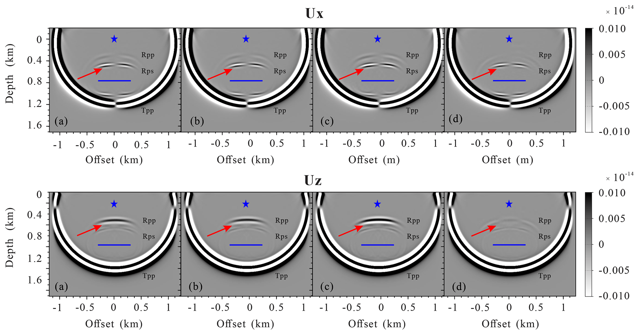
Figure 2 Snapshots of the wavefield components U_x and U_z for a single horizontal fracture model at 280 ms: (a) the PLSM-based poroelastic modeling, (b) the VLSM-based viscoelastic modeling, (c) the LVLSM-based elastic modeling, and (d) the HVLSM-based elastic modeling. The blue asterisk and line represent the source and the fracture, respectively.

If we assume that the interface of the fracture is normal to the z axis (fracture normal vector n is (0,0,1)), substituting Eq. (3) into Eq. (10), we can obtain the nonzero element of the exceeded fracture strain tensor:

$$\begin{array}{}\text{(11)}& \begin{array}{rl}& {\mathit{\epsilon }}_{xz}^c={\displaystyle \frac{S}{V}}{Z}_{\mathrm{T}}{\mathit{\sigma }}_{xz},\\ & {\mathit{\epsilon }}_{yz}^c={\displaystyle \frac{S}{V}}{Z}_{\mathrm{T}}{\mathit{\sigma }}_{yz},\\ & {\mathit{\epsilon }}_{zz}^c={\displaystyle \frac{S}{V}}\left(Z_{\mathrm{N}}{\mathit{\sigma }}_{zz}+Z_X{\mathit{\epsilon }}_{xx}^{\mathrm{b}}\right).\end{array}\end{array}$$

For simplicity, we use an abbreviated Voigt notation for the stresses, strains, and stiffness and compliance tensors, and rewrite the Eqs. (9) and (11) as

$$\begin{array}{}\text{(12)}& {\displaystyle }{\widehat{\mathit{\epsilon }}}^{\mathrm{b}}={\widehat{\mathbf{S}}}^{\mathrm{b}}\widehat{\mathit{\sigma }},\text{(13)}& {\displaystyle }{\widehat{\mathit{\epsilon }}}^c={\displaystyle \frac{S}{V}}\left({\widehat{\mathbf{Z}}}^{\mathrm{I}}\widehat{\mathit{\sigma }}+{\widehat{\mathbf{Z}}}^{\mathrm{II}}\widehat{\mathit{\epsilon }}\right)={\displaystyle \frac{S}{V}}\left({\widehat{\mathbf{Z}}}^{\mathrm{I}}+{\widehat{\mathbf{Z}}}^{\mathrm{II}}{\widehat{\mathbf{S}}}^{\mathrm{b}}\right)\widehat{\mathit{\sigma }},\end{array}$$

where $\widehat{\mathit{\epsilon }}={\left[{\mathit{\epsilon }}_{xx},{\mathit{\epsilon }}_{yy},{\mathit{\epsilon }}_{zz},\mathrm{2}{\mathit{\epsilon }}_{yz},\mathrm{2}{\mathit{\epsilon }}_{xz},\mathrm{2}{\mathit{\epsilon }}_{xy}\right]}^{\mathrm{T}}$ is the strain matrix, $\widehat{\mathit{\sigma }}={\left[{\mathit{\sigma }}_{xx},{\mathit{\sigma }}_{yy},{\mathit{\sigma }}_{zz},{\mathit{\sigma }}_{yz},{\mathit{\sigma }}_{xz},{\mathit{\sigma }}_{xy}\right]}^{\mathrm{T}}$ is the stress matrix, and ${\widehat{\mathbf{S}}}^{\mathrm{b}}$ is the compliance matrix of background. Note that in this paper the “∧” symbol is used to indicate matrices to distinguish them from tensors, which is used to distinguish a tensor. The 6×6 fracture compliance matrix ${\widehat{\mathbf{Z}}}^{\mathrm{I}}$ and additional dimensionless matrix ${\widehat{\mathbf{Z}}}^{\mathrm{II}}$ according to the Voigt notation are defined as

$$\begin{array}{}\text{(14)}& \begin{array}{rl}& {\widehat{\mathbf{Z}}}^{\mathrm{I}}=\left[\begin{array}{cccccc}\mathrm{0}& \mathrm{0}& \mathrm{0}& \mathrm{0}& \mathrm{0}& \mathrm{0}\\ \mathrm{0}& \mathrm{0}& \mathrm{0}& \mathrm{0}& \mathrm{0}& \mathrm{0}\\ \mathrm{0}& \mathrm{0}& Z_{\mathrm{N}}& \mathrm{0}& \mathrm{0}& \mathrm{0}\\ \mathrm{0}& \mathrm{0}& \mathrm{0}& Z_{\mathrm{T}}& \mathrm{0}& \mathrm{0}\\ \mathrm{0}& \mathrm{0}& \mathrm{0}& \mathrm{0}& Z_{\mathrm{T}}& \mathrm{0}\\ \mathrm{0}& \mathrm{0}& \mathrm{0}& \mathrm{0}& \mathrm{0}& \mathrm{0}\end{array}\right],\\ & {\widehat{\mathbf{Z}}}^{\mathrm{II}}=\left[\begin{array}{cccccc}\mathrm{0}& \mathrm{0}& \mathrm{0}& \mathrm{0}& \mathrm{0}& \mathrm{0}\\ \mathrm{0}& \mathrm{0}& \mathrm{0}& \mathrm{0}& \mathrm{0}& \mathrm{0}\\ Z_X& \mathrm{0}& \mathrm{0}& \mathrm{0}& \mathrm{0}& \mathrm{0}\\ \mathrm{0}& \mathrm{0}& \mathrm{0}& \mathrm{0}& \mathrm{0}& \mathrm{0}\\ \mathrm{0}& \mathrm{0}& \mathrm{0}& \mathrm{0}& \mathrm{0}& \mathrm{0}\\ \mathrm{0}& \mathrm{0}& \mathrm{0}& \mathrm{0}& \mathrm{0}& \mathrm{0}\end{array}\right].\end{array}\end{array}$$

The average strain in a homogeneous porous rock containing single fracture can be expressed as the sum of the strains of background and the fractures:

$$\begin{array}{}\text{(15)}& \widehat{\mathit{\epsilon }}={\widehat{\mathit{\epsilon }}}^{\mathrm{b}}+{\widehat{\mathit{\epsilon }}}^c.\end{array}$$

Substituting Eqs. (12) and (13) into Eq. (15), we can obtain the average strain matrix:

$$\begin{array}{}\text{(16)}& \widehat{\mathit{\epsilon }}=\left[{\widehat{\mathbf{S}}}^{\mathrm{b}}+{\displaystyle \frac{S}{V}}\left({\widehat{\mathbf{Z}}}^{\mathrm{I}}+{\widehat{\mathbf{Z}}}^{\mathrm{II}}{\widehat{\mathbf{S}}}^{\mathrm{b}}\right)\right]\widehat{\mathit{\sigma }}.\end{array}$$

Thus, the effective stiffness matrix C can be expressed as

$$\begin{array}{}\text{(17)}& \mathbf{C}={\left[{\widehat{\mathbf{S}}}^{\mathrm{b}}+{\displaystyle \frac{S}{V}}\left({\widehat{\mathbf{Z}}}^{\mathrm{I}}+{\widehat{\mathbf{Z}}}^{\mathrm{II}}{\widehat{\mathbf{S}}}^{\mathrm{b}}\right)\right]}^{-\mathrm{1}}.\end{array}$$

The effective stiffness matrix of case of an inclined fracture can be obtained by rotating the coordinate axis to keep z axis perpendicular to fracture interface. We define the inclined fracture as having an angle φ and an azimuth angle θ, and then the rotation matrix can be obtained as

$$\begin{array}{}\text{(18)}& \widehat{\mathbf{R}}=\left[\begin{array}{ccc}\cos \mathit{\theta }\cos \mathit{\phi }& -\sin \mathit{\theta }& \cos \mathit{\theta }\sin \mathit{\phi }\\ \sin \mathit{\theta }\cos \mathit{\phi }& \cos \mathit{\theta }& \sin \mathit{\theta }\sin \mathit{\phi }\\ -\sin \mathit{\phi }& \mathrm{0}& \cos \mathit{\phi }\end{array}\right],\end{array}$$

as well as the corresponding stress bond matrix ${\widehat{\mathbf{A}}}_{\mathit{\sigma }}\left(\widehat{\mathbf{R}}\right)$ and strain bond matrix ${\widehat{\mathbf{A}}}_{\mathit{\epsilon }}\left(\widehat{\mathbf{R}}\right)$. The new stress matrix ${\widehat{\mathit{\epsilon }}}^{\prime }$ and strain matrix ${\widehat{\mathit{\sigma }}}^{\prime }$ can be expressed as

$$\begin{array}{}\text{(19)}& {\widehat{\mathit{\epsilon }}}^{\prime }={\widehat{\mathbf{A}}}_{\mathit{\epsilon }}{\mathit{\epsilon }}^{\prime },{\widehat{\mathit{\sigma }}}^{\mathbf{\prime }}={\widehat{\mathbf{A}}}_{\mathit{\sigma }}{\mathit{\sigma }}^{\prime }.\end{array}$$

By substituting Eq. (19) into Eq. (13), the new exceed fracture strain matrix can be obtained:

$$\begin{array}{}\text{(20)}& {\widehat{\mathit{\epsilon }}}^c={\displaystyle \frac{S}{V}}{\widehat{\mathbf{A}}}_{\mathit{\epsilon }}\left({\widehat{\mathbf{Z}}}^{\mathrm{I}}+{\widehat{\mathbf{Z}}}^{\mathrm{II}}{\widehat{\mathbf{S}}}^{\mathrm{b}}\right){\widehat{\mathbf{A}}}_{\mathit{\epsilon }}^{\mathrm{T}}\widehat{\mathit{\sigma }}.\end{array}$$

Finally, substituting Eqs. (12) and (20) into Eq. (15), the average strain matrix of each numerical cell containing discretely distributed fractures with the same arbitrary direction can be expressed as

$$\begin{array}{}\text{(21)}& \widehat{\mathit{\epsilon }}=\left[{\widehat{\mathbf{S}}}^{\mathrm{b}}+{\displaystyle \frac{S}{V}}{\widehat{\mathbf{A}}}_{\mathit{\epsilon }}\left({\widehat{\mathbf{Z}}}^{\mathrm{I}}+{\widehat{\mathbf{Z}}}^{\mathrm{II}}{\widehat{\mathbf{S}}}^{\mathrm{b}}\right){\widehat{\mathbf{A}}}_{\mathit{\epsilon }}^{\mathrm{T}}\right]\widehat{\mathit{\sigma }},\end{array}$$

and the corresponding effective stiffness matrix C is

$$\begin{array}{}\text{(22)}& \mathbf{C}={\left[{\widehat{\mathbf{S}}}^{\mathrm{b}}+{\displaystyle \frac{S}{V}}{\widehat{\mathbf{A}}}_{\mathit{\epsilon }}\left({\widehat{\mathbf{Z}}}^{\mathrm{I}}+{\widehat{\mathbf{Z}}}^{\mathrm{II}}{\widehat{\mathbf{S}}}^{\mathrm{b}}\right){\widehat{\mathbf{A}}}_{\mathit{\epsilon }}^{\mathrm{T}}\right]}^{-\mathrm{1}}.\end{array}$$

If the background media is isotropic, the C can be simplified as

$$\begin{array}{}\text{(23)}& \mathbf{C}={\mathbf{C}}^{\mathrm{iso}}{\left[\mathit{I}+{\displaystyle \frac{S}{V}}{\widehat{\mathbf{A}}}_{\mathit{\epsilon }}\left({\widehat{\mathbf{Z}}}^{\mathrm{I}}{\mathbf{C}}^{\mathrm{iso}}+{\widehat{\mathbf{Z}}}^{\mathrm{II}}\right){\widehat{\mathbf{A}}}_{\mathit{\epsilon }}^{\mathrm{T}}\right]}^{-\mathrm{1}}.\end{array}$$

If we ignore the interaction between different fractures and the FPD along the fracture interfaces, the result can be easily extended to the case of multiple sets of discretely distributed large-scale fractures with arbitrary orientation:

$$\begin{array}{}\text{(24)}& \mathbf{C}={\mathbf{C}}^{\mathrm{iso}}{\left[\mathit{I}+\sum _{r=\mathrm{1}}^{N_c}{\displaystyle \frac{S_r}{V}}{\widehat{\mathbf{A}}}_{\mathit{\epsilon }r}\left({\widehat{\mathbf{Z}}}_r^{\mathrm{I}}{\mathbf{C}}^{\mathrm{iso}}+{\widehat{\mathbf{Z}}}_r^{\mathrm{II}}\right){\widehat{\mathbf{A}}}_{\mathit{\epsilon }r}^{\mathrm{T}}\right]}^{-\mathrm{1}},\end{array}$$

where N_c is total number of the fracture directions and the subscript r denotes the rth direction. The derived effective stiffness matrix is to be employed in the viscoelastic finite-difference modeling of discretely distributed large-scale fractures in porous rock.

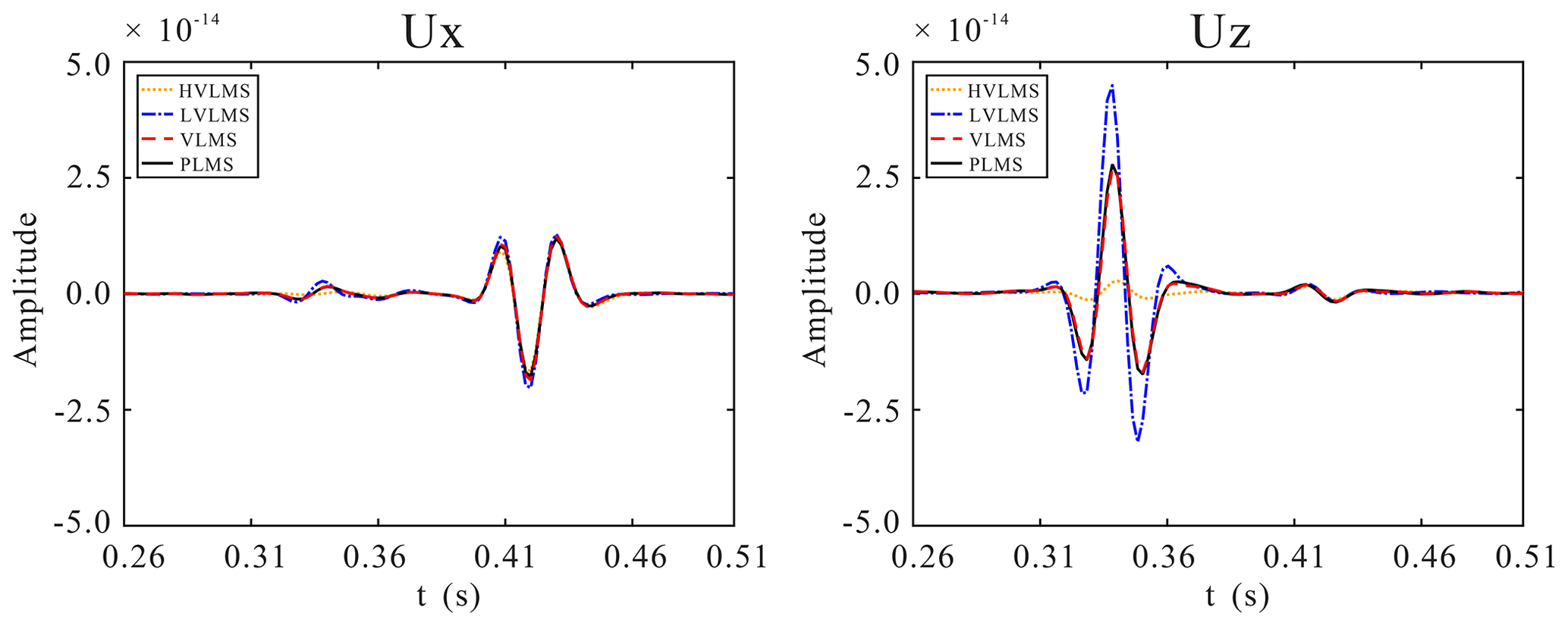
Figure 3 Comparison of 1-D seismograms components U_x and U_z at (1200 m, 0 m) for a single horizontal fracture model.

Since the local-effective-medium theory assumes that the real structure of the fractured porous rock is substituted by ideal continua, the balance equations of classical continuum mechanics can be applied without considering the discontinuity at the fracture interfaces, and the constitutive equations can be characterized by the effective viscoelastic stiffness. Combined with the effective complex-valued and frequency-dependent tilted transversely isotropic (TTI) viscoelastic stiffness, the 2-D frequency-domain second-order heterogeneous governing equations with a perfectly matched layer (PML) of fractured porous rock can be expressed as

$$\begin{array}{}\text{(25)}& \begin{array}{rl}{\mathit{\omega }}^{\mathrm{2}}\mathit{\rho }{u}_x& +{\displaystyle \frac{\mathrm{1}}{{\mathit{\xi }}_x}}{\partial }_x\left({\displaystyle \frac{c_{\mathrm{11}}}{{\mathit{\xi }}_x}}{\partial }_x{u}_x+{\displaystyle \frac{c_{\mathrm{13}}}{{\mathit{\xi }}_z}}{\partial }_z{u}_z+{\displaystyle \frac{c_{\mathrm{15}}}{{\mathit{\xi }}_z}}{\partial }_z{u}_x+{\displaystyle \frac{c_{\mathrm{15}}}{{\mathit{\xi }}_x}}{\partial }_x{u}_z\right)\\ & +{\displaystyle \frac{\mathrm{1}}{{\mathit{\xi }}_z}}{\partial }_z\left({\displaystyle \frac{c_{\mathrm{15}}}{{\mathit{\xi }}_x}}{\partial }_x{u}_x+{\displaystyle \frac{c_{\mathrm{35}}}{{\mathit{\xi }}_z}}{\partial }_z{u}_z+{\displaystyle \frac{c_{\mathrm{55}}}{{\mathit{\xi }}_z}}{\partial }_z{u}_x+{\displaystyle \frac{c_{\mathrm{55}}}{{\mathit{\xi }}_x}}{\partial }_x{u}_z\right)\\ & =\mathrm{0},\\ {\mathit{\omega }}^{\mathrm{2}}\mathit{\rho }{u}_z& +{\displaystyle \frac{\mathrm{1}}{{\mathit{\xi }}_x}}{\partial }_x\left({\displaystyle \frac{c_{\mathrm{15}}}{{\mathit{\xi }}_x}}{\partial }_x{u}_x+{\displaystyle \frac{c_{\mathrm{35}}}{{\mathit{\xi }}_z}}{\partial }_z{u}_z+{\displaystyle \frac{c_{\mathrm{55}}}{{\mathit{\xi }}_z}}{\partial }_z{u}_x+{\displaystyle \frac{c_{\mathrm{55}}}{{\mathit{\xi }}_x}}{\partial }_x{u}_z\right)\\ & +{\displaystyle \frac{\mathrm{1}}{{\mathit{\xi }}_z}}{\partial }_z\left({\displaystyle \frac{c_{\mathrm{13}}}{{\mathit{\xi }}_x}}{\partial }_x{u}_x+{\displaystyle \frac{c_{\mathrm{33}}}{{\mathit{\xi }}_z}}{\partial }_z{u}_z+{\displaystyle \frac{c_{\mathrm{35}}}{{\mathit{\xi }}_z}}{\partial }_z{u}_x+{\displaystyle \frac{c_{\mathrm{35}}}{{\mathit{\xi }}_x}}{\partial }_x{u}_z\right)\\ & =\mathrm{0},\end{array}\end{array}$$

where u_x and u_z are the horizontal and vertical components of particle displacement vector, ρ is the effective density, c_ij represents the components of complex-valued and frequency-dependent effective stiffness matrix, and ξ_x and ξ_z are the frequency-domain PML damping functions.

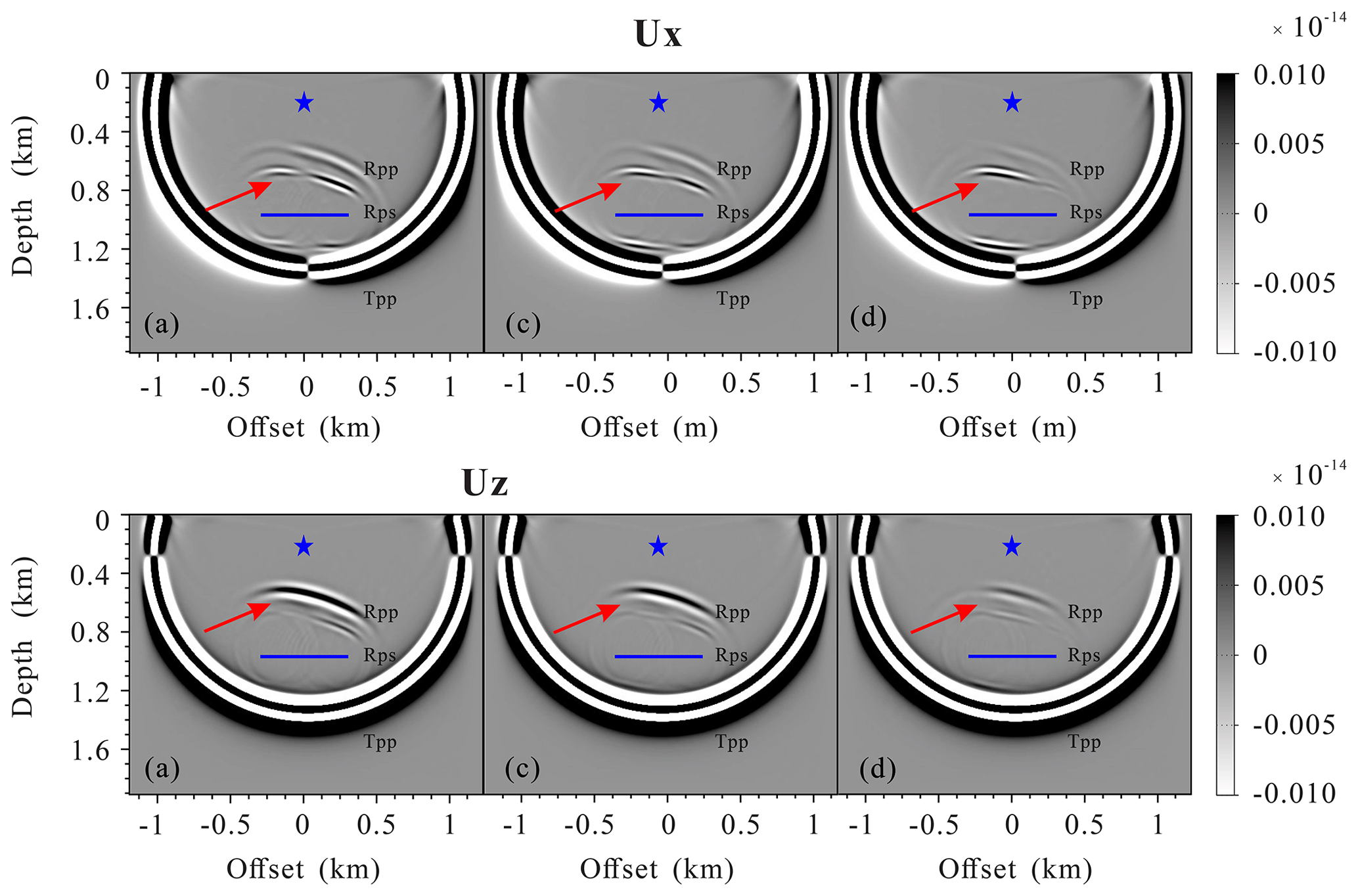
Figure 4 Snapshots of the wavefields components U_x and U_z for a single inclined fracture model at 280 ms: (a) the PLSM-based poroelastic modeling, (b) the VLSM-based viscoelastic modeling, (c) the LVLSM-based elastic modeling, and (d) the HVLSM-based elastic modeling. The blue asterisk and line represent the source and the fracture, respectively.

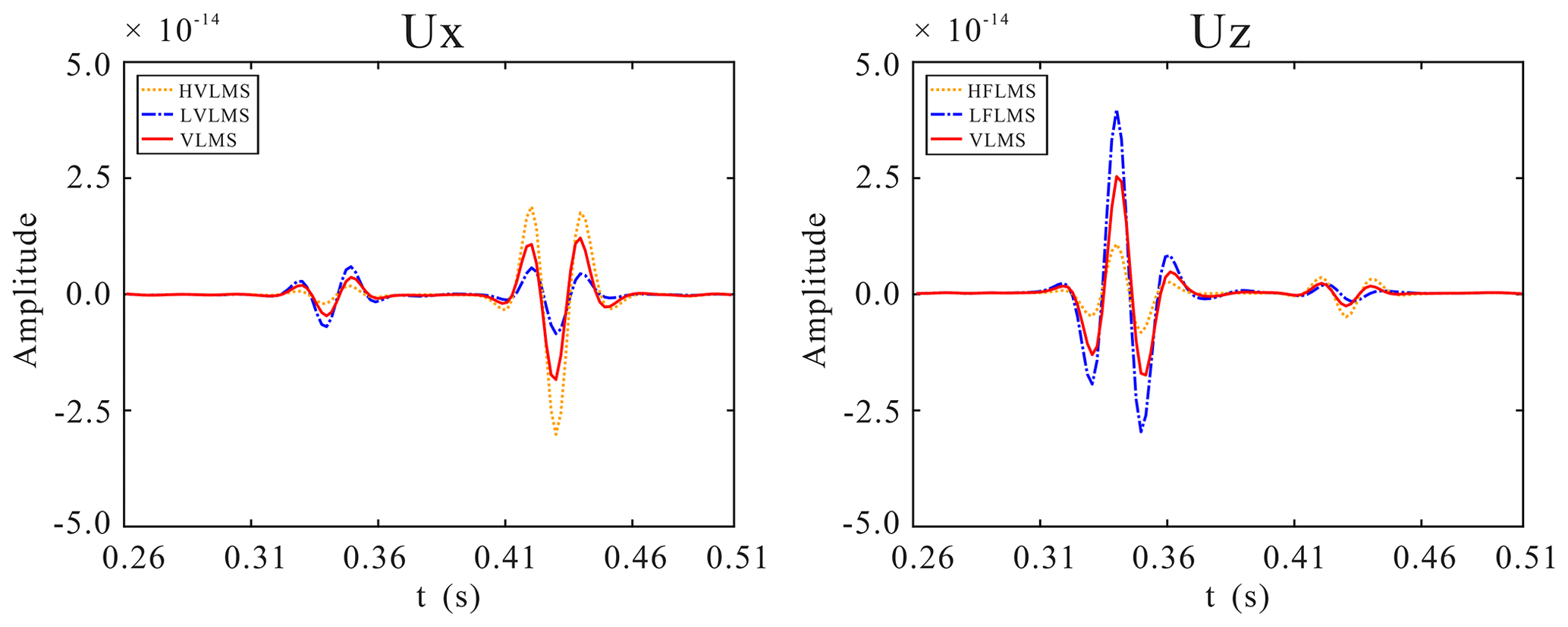
Figure 5 Comparison of 1-D seismograms components U_x and U_z at (1000, 0 m) for a single inclined fracture model.

In time domain, the governing equations are integral differential equations, which require special processing for the convolution operations, resulting in high computational costs. Although the problem can be relieved by memory functions, it still requires high memory requirements. Instead, the governing equations can be straightforwardly solved using FDFD. To efficiently and accurately model seismic wave propagation in fluid-saturated fractured porous rock, we solve the second-order heterogeneous governing equations with the mixed-grid-stencil FDFD method (Jo et al., 1996; Hustedt et al., 2004). The mixed system of governing equations is formulated by combining the classical Cartesian coordinate system (CS) and the 45° rotated coordinate system (RS):

$$\begin{array}{}\text{(26)}& \begin{array}{rl}{\mathit{\omega }}^{\mathrm{2}}\mathit{\rho }{u}_x& +w_{\mathrm{1}}\left(A_c{u}_x+B_c{u}_z\right)\\ & +\left(\mathrm{1}-w_{\mathrm{1}}\right)\left(A_r{u}_x+B_r{u}_z\right)=\mathrm{0},\\ {\mathit{\omega }}^{\mathrm{2}}\mathit{\rho }{u}_z& +w_{\mathrm{1}}\left(C_c{u}_x+D_c{u}_z\right)\\ & +\left(\mathrm{1}-w_{\mathrm{1}}\right)\left(C_r{u}_x+D_r{u}_z\right)=\mathrm{0},\end{array}\end{array}$$

where the optimal averaging coefficient w₁=0.5461 (Jo et al., 1996). The coefficients A_c, B_c, C_c, D_c and A_r, B_r, C_r, D_r are functions of the damping functions, effective stiffness coefficients, and spatial derivative operators, and the detailed expressions are given in Appendix A. We follow Hustedt et al. (2004) and Liu et al. (2018) to discretize the derivative operation on the mixed systems using the mixed-grid stencil. After discretization and arrangement, the mixed system of governing equations can be written in matrix from as

$$\begin{array}{}\text{(27)}& \begin{array}{rl}& \left[\begin{array}{ll}\mathbf{M}+w_{\mathrm{1}}{\mathbf{A}}_c+\left(\mathrm{1}-w_{\mathrm{1}}\right){\mathbf{A}}_r& w_{\mathrm{1}}{\mathbf{B}}_c+\left(\mathrm{1}-w_{\mathrm{1}}\right){\mathbf{B}}_r\\ w_{\mathrm{1}}{\mathbf{C}}_c+\left(\mathrm{1}-w_{\mathrm{1}}\right){\mathbf{C}}_r& \mathbf{M}+w_{\mathrm{1}}{\mathbf{D}}_c+\left(\mathrm{1}-w_{\mathrm{1}}\right){\mathbf{D}}_r\end{array}\right]\\ & \left[\begin{array}{l}{\mathit{u}}_x\\ {\mathit{u}}_z\end{array}\right]=\left[\begin{array}{l}\mathrm{0}\\ \mathrm{0}\end{array}\right],\end{array}\end{array}$$

where M denotes the diagonal mass matrix of coefficients ω²ρ, and blocks A_c, B_c, C_c, D_c and A_r, B_r, C_r, D_r form the stiffness matrices for the CS and RS stencils, respectively, and the corresponding coefficients of submatrices are given in Appendix B.

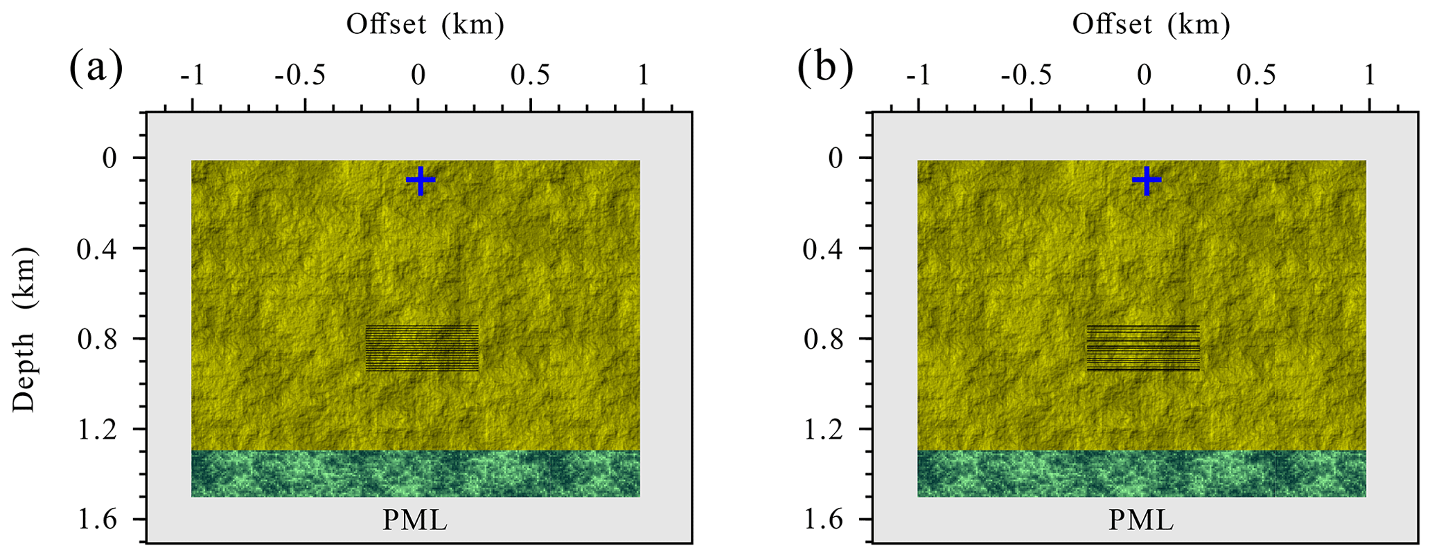
Figure 6 Schematic diagram of the fractured reservoir model with a set of aligned horizontal fractures: (a) regular distribution and (b) random distribution. The black segments present the fracture system. The extension of each fracture is 500 m.

To improve the modeling accuracy of the mixed-grid stencil, the acceleration term ω²ρ is approximated using a weighted average over the mixed operator stencil nodes:

$$\begin{array}{}\text{(28)}& \begin{array}{rl}{\left[{\mathit{\omega }}^{\mathrm{2}}\mathit{\rho }\right]}_{i,j}& \approx {\mathit{\omega }}^{\mathrm{2}}\left[w_{m\mathrm{1}}{\mathit{\rho }}_{i,j}\right.\\ & +w_{m\mathrm{2}}\left({\mathit{\rho }}_{i+\mathrm{1},j}+{\mathit{\rho }}_{i-\mathrm{1},j}+{\mathit{\rho }}_{i,j+\mathrm{1}}+{\mathit{\rho }}_{i,j-\mathrm{1}}\right)\\ & +w_{m\mathrm{3}}\left({\mathit{\rho }}_{i+\mathrm{1},j+\mathrm{1}}+{\mathit{\rho }}_{i-\mathrm{1},j-\mathrm{1}}+{\mathit{\rho }}_{i-\mathrm{1},j+\mathrm{1}}\right.\\ & \left.\left.+{\mathit{\rho }}_{i+\mathrm{1}j-\mathrm{1}}\right)\right],\end{array}\end{array}$$

where the optimal coefficients w_m1=0.6248, w_m2=0.09381, and $w_{m\mathrm{3}}=\left(\mathrm{1}-w_{m\mathrm{1}}-\mathrm{4}{w}_{m\mathrm{2}}\right)/\mathrm{4}$ are computed by Jo et al. (1996).

Figure 7 Seismogram components U_x and U_z of the fractured reservoir model with a set of regularly distributed aligned horizontal fractures calculated using (a) the LVLSM, (b) the VLSM, and (c) the HVLSM. A and B are the scattered P wave from top and bottom, respectively; C and D are the scattered converted shear S wave from top and bottom, respectively; and F and G are the reflected P wave and shear converted S wave, respectively.

In order to assess the FPD effects on the seismic response, a similar procedure can be adopted in the implementation of elastic modeling by replacing the frequency-dependent fracture compliances with its low- or high-frequency limit compliances. The main advantage of our VLSM-based modeling scheme over poroelastic modeling schemes is that the fractured domain can be modeled using a viscoelastic solid, while the rest of the domain can be modeled using an elastic solid.

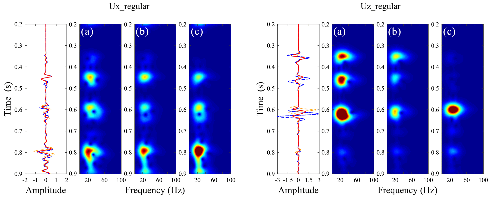
Figure 8 Time–frequency distributions of the middle trace for (b) the LVLSM, (c) the PLSM, and (d) the HVLSM cases in Fig. 7.

Figure 9 Seismogram components U_x and U_z of the fractured reservoir model with a set of randomly distributed aligned horizontal fractures calculated using (a) the LVLSM, (b) the VLSM, and (c) the HVLSM. A and B are the scattered P wave from top and bottom, respectively; C and D are the scattered converted shear S wave from top and bottom, respectively; and F and G are the reflected P wave and shear converted S wave, respectively.

3.2 Poroelastic modeling based on PLSM

The poroelastic modeling means that we numerically solve Biot's equations and adopt an explicit implementation of the PLSM across each fracture instead of using the effective media theory. Hence, the poroelastic modeling can naturally deal with the FPD between fracture and background and account for its impact on wave scattering. To verify the effectiveness of the viscoelastic modeling based on VLSM, we compared the results obtained from the viscoelastic scheme with those obtained from the poroelastic scheme. Although it is difficult to implement an explicit application of PLSM for an arbitrarily orientated fracture, it is relatively straightforward for a horizontal or vertical fracture. In the following, we outline the poroelastic modeling for a single horizontal fracture embedded in an isotropic homogeneous background with an explicit implementation of the PLSM. In frequency the domain, the governing equations for an isotropic poroelastic media in the absence of fractures can be written as (Biot, 1962)

$$\begin{array}{}\text{(29)}& \begin{array}{rl}& -{\mathit{\omega }}^{\mathrm{2}}\mathit{\rho }{u}_i-{\mathit{\omega }}^{\mathrm{2}}{\mathit{\rho }}_{\mathrm{f}}{w}_i={\partial }_i{\mathit{\sigma }}_{ij},\\ & -{\mathit{\omega }}^{\mathrm{2}}{\mathit{\rho }}_{\mathrm{f}}{u}_i-{\mathit{\omega }}^{\mathrm{2}}{\mathit{\rho }}_w{w}_i+i\mathit{\omega }{\displaystyle \frac{\mathit{\eta }}{\mathit{\kappa }}}{w}_i=-{\partial }_i{P}_{\mathrm{f}},\\ & {\mathit{\sigma }}_{ij}=\left(H_{\mathrm{U}}-\mathrm{2}\mathit{\mu }\right){\partial }_i{u}_i+\mathit{\alpha }M{\partial }_i{w}_i+\mathit{\mu }\left({\partial }_j{u}_i+{\partial }_i{u}_j\right),\\ & -P_{\mathrm{f}}=\mathit{\alpha }M{\partial }_i{u}_i+M{\partial }_i{w}_i.\end{array}\end{array}$$

In the presence of fractures, the spatial derivative of stress remains unchanged. However, due to the discontinuity of particle displacements across the fracture interface, its spatial derivative consists of two parts, i.e., the background and the fracture:

$$\begin{array}{}\text{(30)}& \begin{array}{rl}& {\displaystyle \frac{\partial u_x}{\partial z}}={\left({\displaystyle \frac{\partial u_x}{\partial z}}\right)}_{\mathrm{BG}}+{\left({\displaystyle \frac{\partial u_x}{\partial z}}\right)}_{\mathrm{FR}},\\ & {\displaystyle \frac{\partial u_z}{\partial z}}={\left({\displaystyle \frac{\partial u_z}{\partial z}}\right)}_{\mathrm{BG}}+{\left({\displaystyle \frac{\partial u_z}{\partial z}}\right)}_{\mathrm{FR}},\\ & {\displaystyle \frac{\partial w_z}{\partial z}}={\left({\displaystyle \frac{\partial w_z}{\partial z}}\right)}_{\mathrm{BG}}+{\left({\displaystyle \frac{\partial w_z}{\partial z}}\right)}_{\mathrm{FR}}.\end{array}\end{array}$$

The spatial derivative of the background is described by the Eq. (29):

$$\begin{array}{}\text{(31)}& \begin{array}{rl}& {\left({\displaystyle \frac{\partial u_x}{\partial x}}\right)}_{\mathrm{BG}}={\displaystyle \frac{H_{\mathrm{D}}}{\mathrm{4}\mathit{\mu }\left(H_{\mathrm{D}}-\mathit{\mu }\right)}}{\mathit{\sigma }}_{xx}-{\displaystyle \frac{H_{\mathrm{D}}-\mathrm{2}\mathit{\mu }}{\mathrm{4}\mathit{\mu }\left(H_{\mathrm{D}}-\mathit{\mu }\right)}}{\mathit{\sigma }}_{zz}\\ & +{\displaystyle \frac{\mathrm{2}\mathit{\alpha }\mathit{\mu }}{\mathrm{4}\mathit{\mu }\left(H_{\mathrm{D}}-\mathit{\mu }\right)}}{P}_{\mathrm{f}},\\ & {\left({\displaystyle \frac{\partial u_z}{\partial z}}\right)}_{\mathrm{BG}}=-{\displaystyle \frac{H_{\mathrm{D}}-\mathrm{2}\mathit{\mu }}{\mathrm{4}\mathit{\mu }\left(H_{\mathrm{D}}-\mathit{\mu }\right)}}{\mathit{\sigma }}_{xx}+{\displaystyle \frac{H_{\mathrm{D}}}{\mathrm{4}\mathit{\mu }\left(H_{\mathrm{D}}-\mathit{\mu }\right)}}{\mathit{\sigma }}_{zz}\\ & +{\displaystyle \frac{\mathrm{2}\mathit{\alpha }\mathit{\mu }}{\mathrm{4}\mathit{\mu }\left(H_{\mathrm{D}}-\mathit{\mu }\right)}}{P}_{\mathrm{f}},\\ & {\left({\displaystyle \frac{\partial w_x}{\partial x}}+{\displaystyle \frac{\partial w_z}{\partial z}}\right)}_{\mathrm{BG}}=-{\displaystyle \frac{\mathrm{2}\mathit{\alpha }\mathit{\mu }}{\mathrm{4}\mathit{\mu }\left(H_{\mathrm{D}}-\mathit{\mu }\right)}}{\mathit{\sigma }}_{xx}\\ & -{\displaystyle \frac{\mathrm{2}\mathit{\alpha }\mathit{\mu }}{\mathrm{4}\mathit{\mu }\left(H_{\mathrm{D}}-\mathit{\mu }\right)}}{\mathit{\sigma }}_{zz}-{\displaystyle \frac{H_{\mathrm{U}}-\mathit{\mu }}{M\left(H_{\mathrm{D}}-\mathit{\mu }\right)}}{P}_{\mathrm{f}}.\end{array}\end{array}$$

The fracture-induced spatial derivative can be obtained based on the PLSM:

$$\begin{array}{}\text{(32)}& \begin{array}{rl}& {\left({\displaystyle \frac{\partial u_x}{\partial z}}\right)}_{\mathrm{FR}}={\displaystyle \frac{\mathrm{\Delta }{u}_x}{\mathrm{\Delta }z}}={\displaystyle \frac{Z_{\mathrm{T}}}{\mathrm{\Delta }z}}{\mathit{\sigma }}_{xz},\\ & {\left({\displaystyle \frac{\partial u_z}{\partial z}}\right)}_{\mathrm{FR}}={\displaystyle \frac{\mathrm{\Delta }{u}_z}{\mathrm{\Delta }z}}={\displaystyle \frac{Z_{{\mathrm{N}}_{\mathrm{D}}}}{\mathrm{\Delta }z}}\left({\mathit{\sigma }}_{zz}+\mathit{\alpha }{P}_{\mathrm{f}}\right),\\ & {\left({\displaystyle \frac{\partial w_z}{\partial z}}\right)}_{\mathrm{FR}}={\displaystyle \frac{\mathrm{\Delta }{w}_z}{\mathrm{\Delta }z}}=-{\displaystyle \frac{Z_{{\mathrm{N}}_{\mathrm{D}}}}{\mathrm{\Delta }z}}\left(\mathit{\alpha }{\mathit{\sigma }}_{zz}+{\displaystyle \frac{H_{\mathrm{U}}}{M}}{P}_{\mathrm{f}}\right).\end{array}\end{array}$$

By substituting Eqs. (31)–(32) into Eq. (30) and the rewritten Eq. (29), we obtain the governing equations for numerical simulation of elastic wave in fractured poroelastic media in matrix form:

$$\begin{array}{}\text{(33)}& -{\mathit{\omega }}^{\mathrm{2}}\widehat{\mathbf{R}}\widehat{\mathit{u}}=\mathrm{\nabla }{\widehat{\mathbf{S}}}^{-\mathrm{1}}{\mathrm{\nabla }}^{\mathrm{T}}\widehat{\mathit{u}},\end{array}$$

where $\widehat{\mathit{u}}={\left(u_x,u_z,w_x,w_z\right)}^{\mathrm{T}}$ is the displacement vector and $\widehat{\mathbf{R}}$, $\widehat{\mathbf{S}}$, and ∇ are the density, compliance, and spatial derivative matrix, respectively. The three matrices in Eq. (33) are defined as

$$\begin{array}{}\text{(34)}& {\displaystyle }\widehat{\mathbf{R}}=\left[\begin{array}{cccc}\mathit{\rho }& \mathrm{0}& {\mathit{\rho }}_{\mathrm{f}}& \mathrm{0}\\ \mathrm{0}& \mathit{\rho }& \mathrm{0}& {\mathit{\rho }}_{\mathrm{f}}\\ {\mathit{\rho }}_{\mathrm{f}}& \mathrm{0}& {\mathit{\rho }}_m& \mathrm{0}\\ \mathrm{0}& {\mathit{\rho }}_{\mathrm{f}}& \mathrm{0}& {\mathit{\rho }}_m\end{array}\right],\left({\mathit{\rho }}_m={\mathit{\rho }}_w-{\displaystyle \frac{i\mathit{\eta }}{\mathit{\omega }\mathit{\kappa }}}\right),\text{(35)}& {\displaystyle }\mathrm{\nabla }=\left[\begin{array}{cccc}{\partial }_x& \mathrm{0}& {\partial }_z& \mathrm{0}\\ \mathrm{0}& {\partial }_z& {\partial }_x& \mathrm{0}\\ \mathrm{0}& \mathrm{0}& \mathrm{0}& {\partial }_x\\ \mathrm{0}& \mathrm{0}& \mathrm{0}& {\partial }_z\end{array}\right],\text{(36)}& {\displaystyle }\widehat{\mathbf{S}}=\left[\begin{array}{cccc}\frac{H_{\mathrm{D}}}{\mathrm{4}\mathit{\mu }\left(H_{\mathrm{D}}-\mathit{\mu }\right)}& -\frac{H_{\mathrm{D}}-\mathrm{2}\mathit{\mu }}{\mathrm{4}\mathit{\mu }\left(H_{\mathrm{D}}-\mathit{\mu }\right)}& \mathrm{0}& -\frac{\mathrm{2}\mathit{\alpha }\mathit{\mu }}{\mathrm{4}\mathit{\mu }\left(H_{\mathrm{D}}-\mathit{\mu }\right)}\\ -\frac{H_{\mathrm{D}}-\mathrm{2}\mathit{\mu }}{\mathrm{4}\mathit{\mu }\left(H_{\mathrm{D}}-\mathit{\mu }\right)}& \frac{H_{\mathrm{D}}}{\mathrm{4}\mathit{\mu }\left(H_{\mathrm{D}}-\mathit{\mu }\right)}+\frac{Z_{{\mathrm{N}}_{\mathrm{D}}}}{\mathrm{\Delta }z}& \mathrm{0}& -\frac{\mathrm{2}\mathit{\alpha }\mathit{\mu }}{\mathrm{4}\mathit{\mu }\left(H_{\mathrm{D}}-\mathit{\mu }\right)}-\frac{\mathit{\alpha }{Z}_{{\mathrm{N}}_{\mathrm{D}}}}{\mathrm{\Delta }z}\\ \mathrm{0}& \mathrm{0}& \frac{\mathrm{1}}{\mathit{\mu }}+\frac{Z_{\mathrm{T}}}{\mathrm{\Delta }z}& \mathrm{0}\\ -\frac{\mathrm{2}\mathit{\alpha }\mathit{\mu }}{\mathrm{4}\mathit{\mu }\left(H_{\mathrm{D}}-\mathit{\mu }\right)}& -\frac{\mathrm{2}\mathit{\alpha }\mathit{\mu }}{\mathrm{4}\mathit{\mu }\left(H_{\mathrm{D}}-\mathit{\mu }\right)}-\frac{\mathit{\alpha }{Z}_{{\mathrm{N}}_{\mathrm{D}}}}{\mathrm{\Delta }z}& \mathrm{0}& -\frac{H_{\mathrm{U}}-\mathit{\mu }}{M\left(H_{\mathrm{D}}-\mathit{\mu }\right)}-\frac{H_{\mathrm{U}}{Z}_{{\mathrm{N}}_{\mathrm{D}}}}{M\mathrm{\Delta }z}\end{array}\right].\end{array}$$

A compact discretized wave equation system that contains only displacement field can be obtained by using second-order difference operators to discretize the new governing equations:

$$\begin{array}{}\text{(37)}& \left[\begin{array}{cccc}{\mathbf{G}}_{\mathrm{11}}& {\mathbf{G}}_{\mathrm{12}}& {\mathbf{G}}_{\mathrm{13}}& {\mathbf{G}}_{\mathrm{14}}\\ {\mathbf{G}}_{\mathrm{21}}& {\mathbf{G}}_{\mathrm{22}}& {\mathbf{G}}_{\mathrm{23}}& {\mathbf{G}}_{\mathrm{24}}\\ {\mathbf{G}}_{\mathrm{31}}& {\mathbf{G}}_{\mathrm{32}}& {\mathbf{G}}_{\mathrm{33}}& {\mathbf{G}}_{\mathrm{34}}\\ {\mathbf{G}}_{\mathrm{41}}& {\mathbf{G}}_{\mathrm{42}}& {\mathbf{G}}_{\mathrm{43}}& {\mathbf{G}}_{\mathrm{44}}\end{array}\right]\left[\begin{array}{c}vec{u}_x\\ vec{u}_z\\ vec{w}_x\\ vec{w}_z\end{array}\right]=\left[\begin{array}{c}\mathrm{0}\\ \mathrm{0}\\ \mathrm{0}\\ \mathrm{0}\end{array}\right],\end{array}$$

where blocks ${\mathbf{G}}_{i,j}\left(i,j=\mathrm{1}\mathrm{\dots }\mathrm{4}\right)$ form the stiffness matrices of the discretized system of the poroelastic wave equations. The poroelastic modeling based on PLSM will be used to validate the other modeling schemes.

4 Numerical examples

In this section, we apply different numerical modeling schemes on three fractured models to examine the FPD effects on seismic wave scattering. We mainly focus on the amplitudes and phases of the scattered and reflected waves.

4.1 Single fracture model

Here, we numerically simulate the scattering of seismic waves from a single fracture embedded in a homogeneous background. The model measures 2000 m × 1500 m with a grid interval of 5 m (namely, the numerical grids size is 401×301) surrounded by a 200 m thick PML boundary. The fracture is parallel to the x axis (a horizontal fracture) and located 750 m directly below the source (1000,30 m), with a 500 m horizontal extension. A Ricker wavelet with a central frequency of 35 Hz is used as the temporal source excitation. The material properties of the fracture and background are given in Table 1, modified from Nakagawa and Schoenberg (2007) and Barbosa et al. (2016a). For comparison, we present the seismic wavefields obtained using the poroelastic modeling based on PLSM, the viscoelastic modeling based on VLSM, and the elastic modeling based on the low-frequency limit of VLSM (LVLSM) and high-frequency limit of VLSM (HVLSM). For the convenience of observation of the impact of the FPD on the scattered P and S wave of the fracture, we apply the pressure source in all four schemes.

Table 1 Physical properties of the materials employed in the numerical modeling.

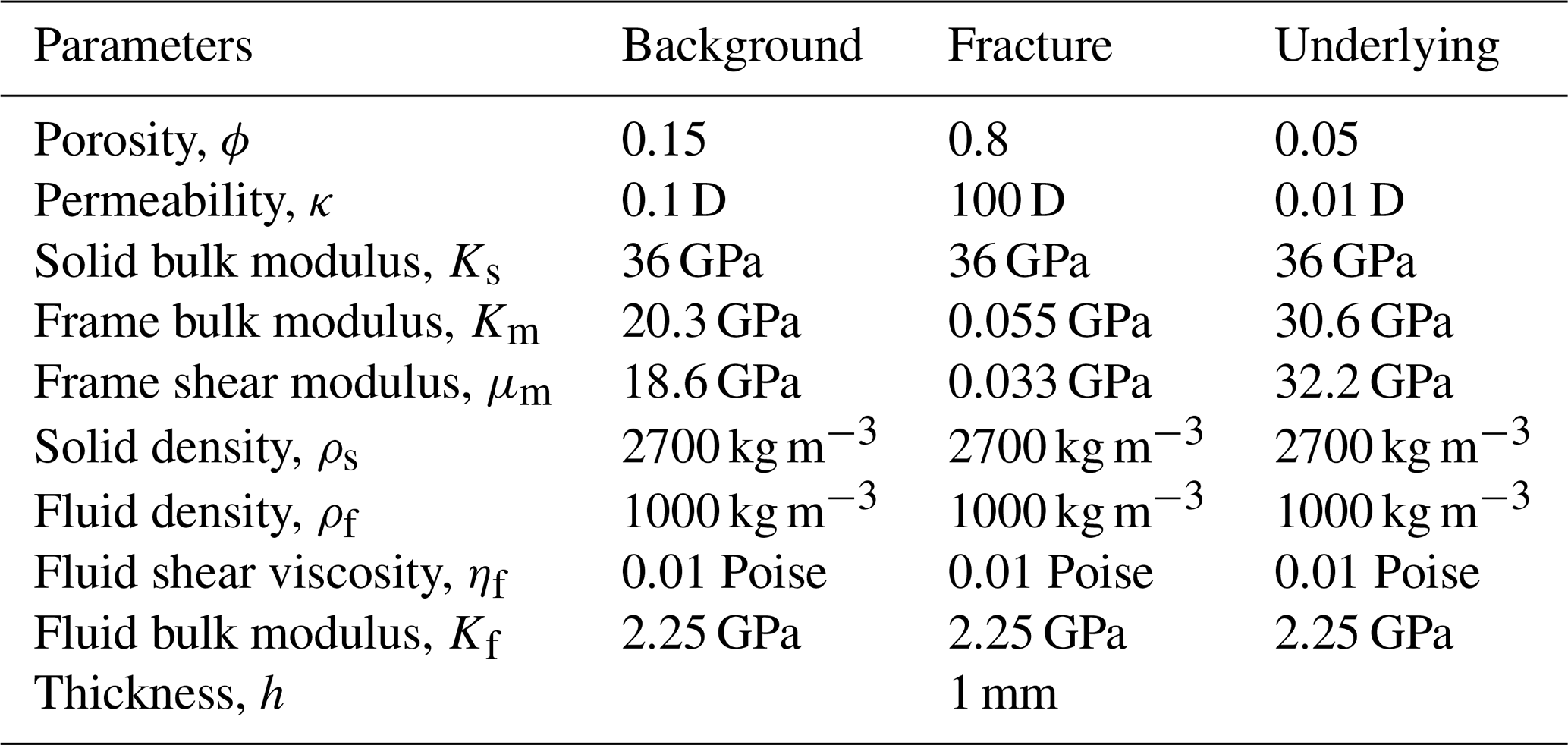
Figure 1 shows the complex-valued and frequency-dependent fracture normal compliance Z_N and dimensionless parameter Z_X computed from Eq. (6). The mechanical compliance of the fracture is strongly controlled by FPD effects. It can be observed that the real part of the fracture normal compliance decreases with the increment of frequency, while the imaginary part has a peak at the characteristic frequency, corresponding to the maximal dispersion. The central frequency (35 Hz) of the Ricker wavelet used for numerical simulation is close to the characteristic frequency (46 Hz), which ensures that the impact of the FPD effects on seismic scattering is significant in the seismic frequency band.

Figure 2 shows the 280 ms snapshots of the displacement fields for the single horizontal fracture model models. The displacement fields are calculated by the PLSM-based poroelastic modeling, the VLSM-based viscoelastic modeling, the LVLSM-based elastic modeling, and the HVLSM-based elastic modeling, respectively. The asterisk represents the source and the blue line represents the fracture. To make the small scattered wave visible, the large amplitude is clipped; thus, the transmitted compressional waves (T_PP), scattered compressional waves (S_PP), and scattered converted waves (S_PS) can be seen clearly. It should be noted that the slow P waves are invisible in the poroelastic modeling, due to the high diffusion and attenuation of slow P waves in the background media. Figure 3 present the comparison of 1-D seismograms at (1200, 0 m).

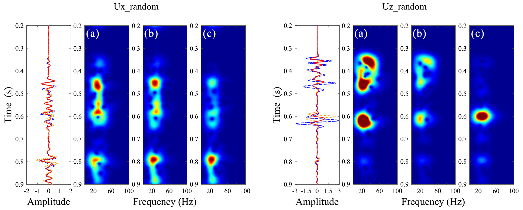
Figure 10 Time–frequency distributions of the middle trace for (b) the LVLSM, (c) the PLSM, and (d) the HVLSM cases in Fig. 9.

We consider the poroelastic modeling as a reference scenario because it can naturally incorporate the FPD effects. Figures 2 and 3 suggest very good agreement between the S_PP amplitude calculated using the PLSM-based and VLSM-based modeling, while the HVLSM-based modeling obviously underestimates the S_PP amplitude, and the LVLSM-based modeling overestimates the S_PP amplitude. This is to be expected, since the scattering behavior of a fracture is mainly controlled by the stiffness contrast with respect to the background. The HVLSM assumes there is insufficient time for fluid exchange at the fracture interface; the fracture behaves as being sealed and the stiffness of the saturated fracture is maximal, resulting in an underestimated stiffness contrast between fracture and background. The LVLSM assumes there is enough time for fluid flow between the fracture and background, and the deformation of the fracture is maximal, resulting in an overestimated stiffness contrast with background. The VLSM derived from poroelastic theory, however, can properly incorporate the FPD effects, leading to a frequency-dependent stiffness contrast equivalent to the PLSM. It can be noted that the S_PP amplitudes obtained using the LVLSM-based modeling are comparable to that of the PLSM-based modeling, because the FPD effects mainly occur at seismic frequencies closer to the low-frequency limit. The S_PP travel time obtained using the four modeling schemes shows good consistency. Figures 2 and 3 also show that the discrepancy of the S_PS amplitudes is almost negligible, because the S wave scattering behavior is mainly controlled by the drained stiffness contrast between the fracture and the background. The comparison of different modeling schemes demonstrates that the VLSM-based viscoelastic modeling can appropriately capture the FPD effects on wave scattering of a fluid-saturated fracture, while the two elastic modeling schemes cannot correctly estimate the scattered waves.

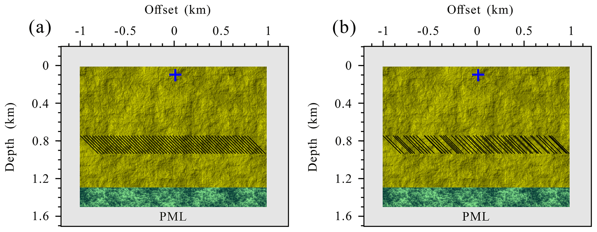
Figure 11 Schematic diagram of the fractured reservoir model with a set of aligned inclined fractures: (a) regular distribution and (b) random distribution. The black segments present the fracture system. The extension of each fracture is 282.8 m.

Figure 12 Seismogram components U_x and U_z of the fractured reservoir model with a set of regularly distributed aligned inclined fractures calculated using (a) the LVLSM, (b) the VLSM, and (c) the HVLSM. A and B are the scattered P wave from top and bottom, respectively; C and D are the scattered converted shear S wave from top and bottom, respectively; and F and G are the reflected P wave and shear converted S wave, respectively.

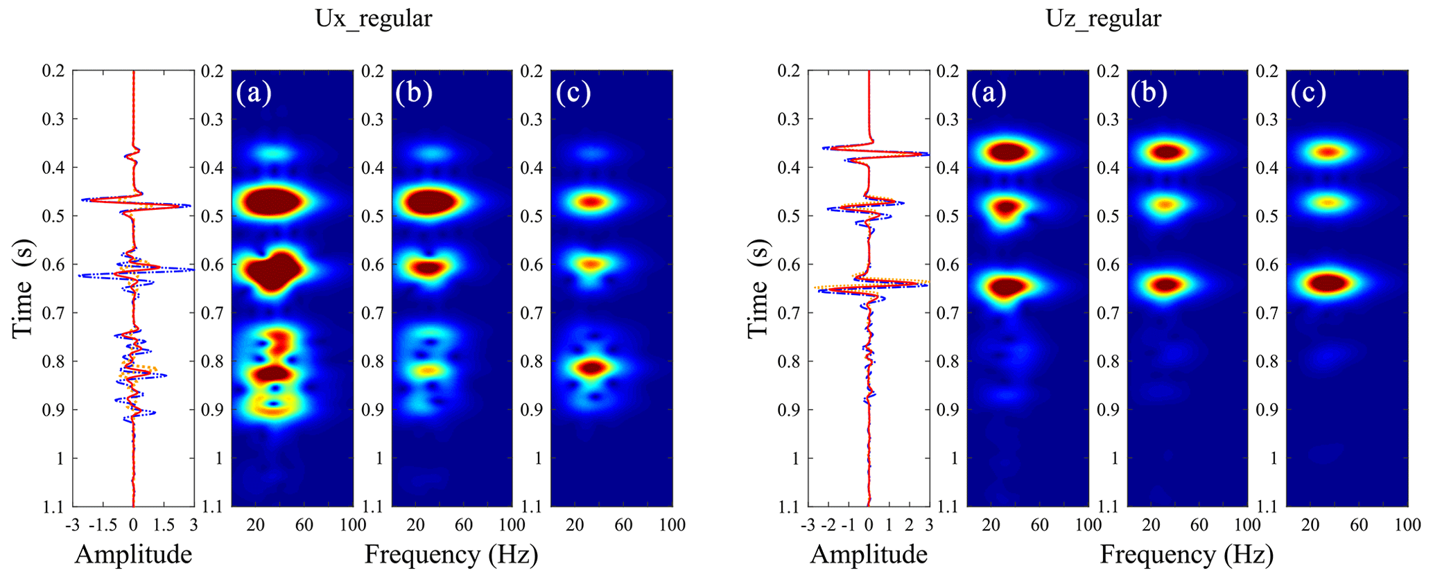
Figure 13 Time–frequency distributions of the middle trace for (b) the LVLSM, (c) the PLSM, and (d) the HVLSM cases in Fig. 12.

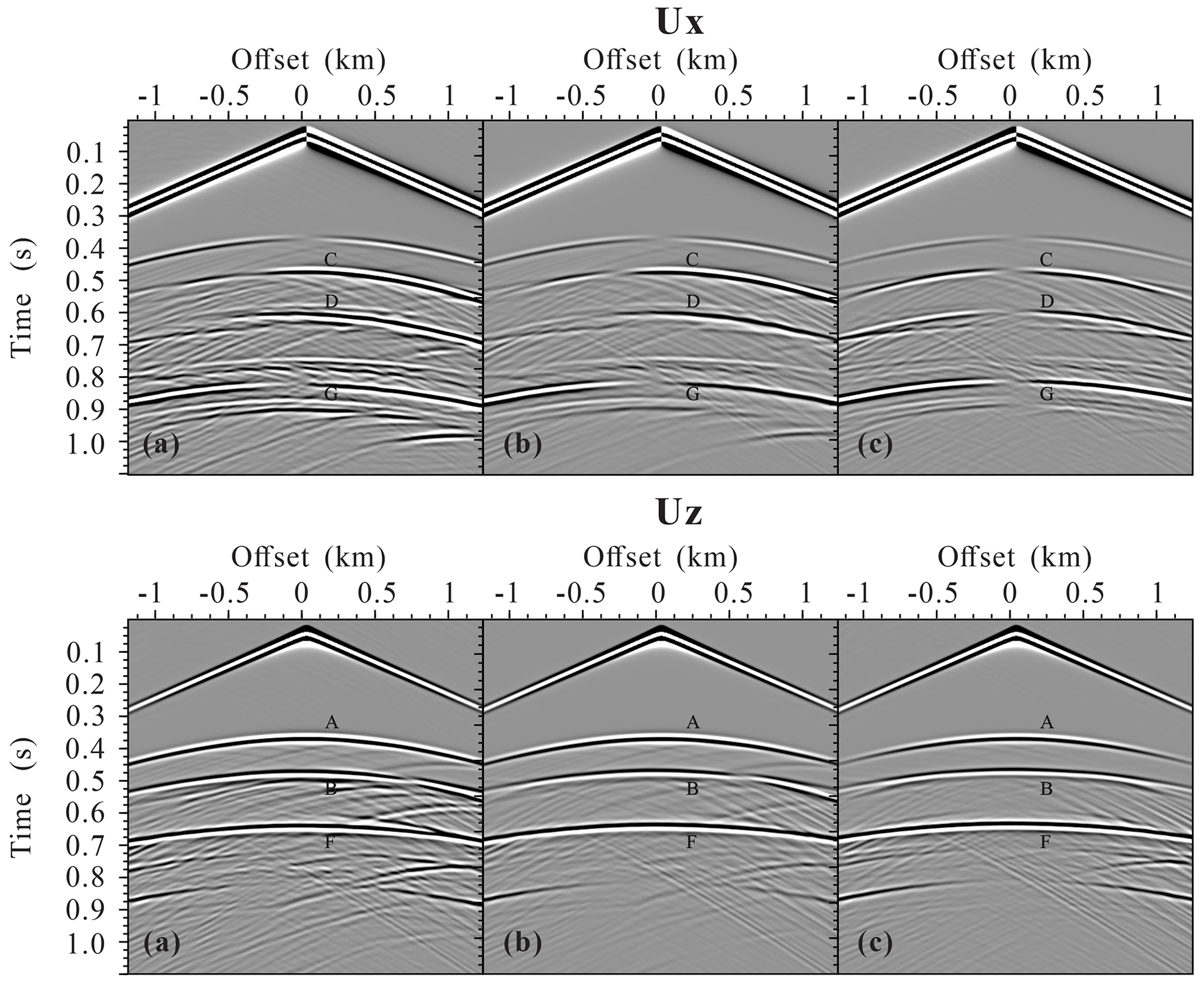
Figure 14 Seismogram components U_x and U_z of the fractured reservoir model with a set of randomly distributed aligned inclined fractures calculated using (a) the LVLSM, (b) the VLSM, and (c) the HVLSM. A and B are the scattered P wave from top and bottom, respectively; C and D are the scattered converted shear S wave from top and bottom, respectively; and F and G are the reflected P wave and shear converted S wave, respectively.

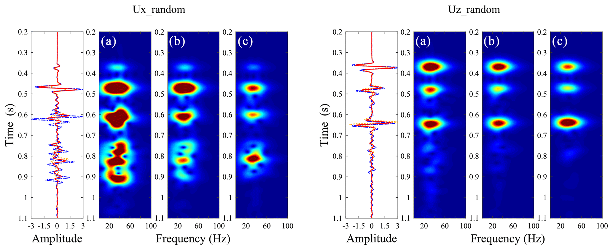
Figure 15 Time–frequency distributions of the middle trace for (b) the LVLSM, (c) the PLSM, and (d) the HVLSM cases in Fig. 14.

The proposed modeling scheme is also applicable to the inclined fracture. Figure 4 shows the 280 ms snapshots of the displacement fields for the single inclined fracture model. Figure 5 is the comparison of 1-D seismograms at (1200, 0 m). Figures 4 and 5 show that both the scattered P and S waves of a single inclined fracture are strongly affected by the FPD effects.

4.2 Fractured reservoir model

In addition to a single fracture, we are more interested in the scattering behavior of discretely distributed fracture system. To this end, we designed two fractured reservoir models containing a set of regularly distributed aligned horizontal fractures and a set of randomly distributed aligned horizontal fractures, respectively, as illustrated in Fig. 6. There are 200 horizontal fractures spread over a space of 200 m, each extending 500 m. The material properties of the fracture, background (yellow region), and underlying (green region) formation are given in Table 1. The model size, grid interval, and source location are the same as those in the previous numerical examples. Though a set of aligned horizontal fracture structures is not practical in the actual subsurface, it helps to illustrate the impact of FPD effects on the amplitude and phase of scattered waves of fractures.

Figure 7 presents the seismograms of the fractured reservoir model with a set of regularly distributed aligned horizontal fractures. The scattered compressional wave (S_PP) and scattered converted wave (S_PS) from the top and bottom of the fractured reservoir, the reflected compressional wave (R_PP), and the converted wave (R_PS) from the underlying formation can be clearly identified. Due to the regular distribution of aligned fractures, the fractured reservoir is equivalent to an anisotropic homogeneous media, and therefore the diffracted wave is generated only at the edges of the fractured reservoir. Similar to the single fracture case, the amplitude of the S_PP from the top and bottom of the fractured reservoir obtained by the HVLSM-based modeling is weakest (underestimated), that obtained by LVLSM-based modeling is strongest (overestimated), and that obtained by the VLSM-based modeling is intermediate. We notice that the S_PP amplitudes from the bottom of the fractured reservoir obtained by the LVLSM-based and HVLSM-based modeling are slightly smaller than those from the top, while the S_PP amplitude from the bottom obtained by the VLSM-based modeling is much smaller than that from the top. This is expected, since the VLSM-based modeling scheme can capture the wave attenuation and dispersion due to the FPD effects between the fracture system and background, while the LVLSM and HVLSM represent non-attenuated and non-dispersive elastic processes. Further evidence for attenuation is that the R_PP amplitudes of the underlying formation calculated by the HVLSM-based and LVLSM-based modeling are almost equal, while the R_PP amplitude calculated by the VLSM-based modeling is much smaller. Figure 7 also shows that the arrival times of S_PP from the bottom and R_PP from underlying formation obtained by the three modeling schemes are different.

To show the trend of frequency-dependent attenuation and dispersion, time–frequency distribution of the middle trace was computed for three modeling schemes. Figure 8 clearly shows that the frequency content and energy of the scattered and reflected waves calculated by VLSM tend to decrease strongly, while the frequency content and energy calculated by HVLSM and LVLSM remain steady. The impact of FPD effects on the S_PS and R_PS is similar to that of the S_PP and R_PP but to a much weaker extent.

In addition to regularly distributed fractures, our proposed modeling scheme can also simulate the wave scattering of randomly distributed fractures. Figure 9 presents the seismograms of the fractured reservoir model with a set of randomly distributed aligned horizontal fractures. Figure 10 presents the time–frequency distributions of the middle trace for three modeling scheme cases in Fig. 9. Due to the random distribution of aligned fractures, the fractured reservoir exhibits a stronger heterogeneity, resulting in a more prevalent diffracted wave (coda wave) in Fig. 9 than in Fig. 7. Except for the diffracted wave, the scattered and reflected waves in the random distribution case are similar to those in the regular distribution case due to the FPD effect. The two fractured reservoir models suggest that the scattered waves from the bottom of the fractured reservoir are attenuated and dispersed by the FPD effects, and the reflected waves can retain the relevant attenuation and dispersion information.

To validate the effectiveness of our proposed modeling scheme in a more practical underground fractured reservoir, we replace a set of aligned horizontal fractures in the original model with a set of aligned inclined fractures, as illustrated in Fig. 11. Figure 12 presents the seismograms of the fractured reservoir model with a set of regularly distributed aligned inclined fractures, and Fig. 13 shows the time–frequency distributions of the middle trace for three modeling schemes. Figures 14 and 15 present the seismograms of the fractured reservoir model with a set of randomly distributed aligned inclined fractures and the time–frequency distributions of the middle trace for three modeling schemes, respectively. All results of PLSM-based modeling capture the influence of FPD effects on the amplitude and phase of scattered waves, validating the effectiveness of our proposed modeling scheme. Figures 12 and 14 also show the different scattering characteristics of the randomly and regularly distributed incline fractures: many coda waves are generated by the randomly distributed fractures due to a stronger heterogeneity.

4.3 Modified Marmousi model

We test the proposed VLSM-based modeling scheme on a more complex modified Marmousi model. To modify the Marmousi model, we generate a porosity model, permeability model, and discrete large-scale fracture system; transform the original P-wave velocity and density into the fluid-saturated bulk and shear modulus of the background by a constant Poisson ratio of 0.5; and finally obtain the grain bulk modulus, the frame bulk, and shear modulus of the background through the Gassmann equation and empirical formula ($K_{\mathrm{m}}={\left(\mathrm{1}-\mathit{\varphi }\right)}^{\frac{\mathrm{3}}{\left(\mathrm{1}-\mathit{\varphi }\right)}}{K}_{\mathrm{s}})$. The input physical properties and elastic modulus models of the modified Marmousi model are present in Fig. 11. The fluid density, bulk modulus, and viscosity are the same as in Table 1. The model size is 4250 m× 1750 m with a grid interval of 5 m and a 100 m thick PML boundary. The source is located at the surface (2125, 0 m). A Ricker wavelet with a central frequency of 25 Hz is used as the temporal source excitation.

Figure 16 The physical properties and elastic modulus models of the modified Marmousi model.

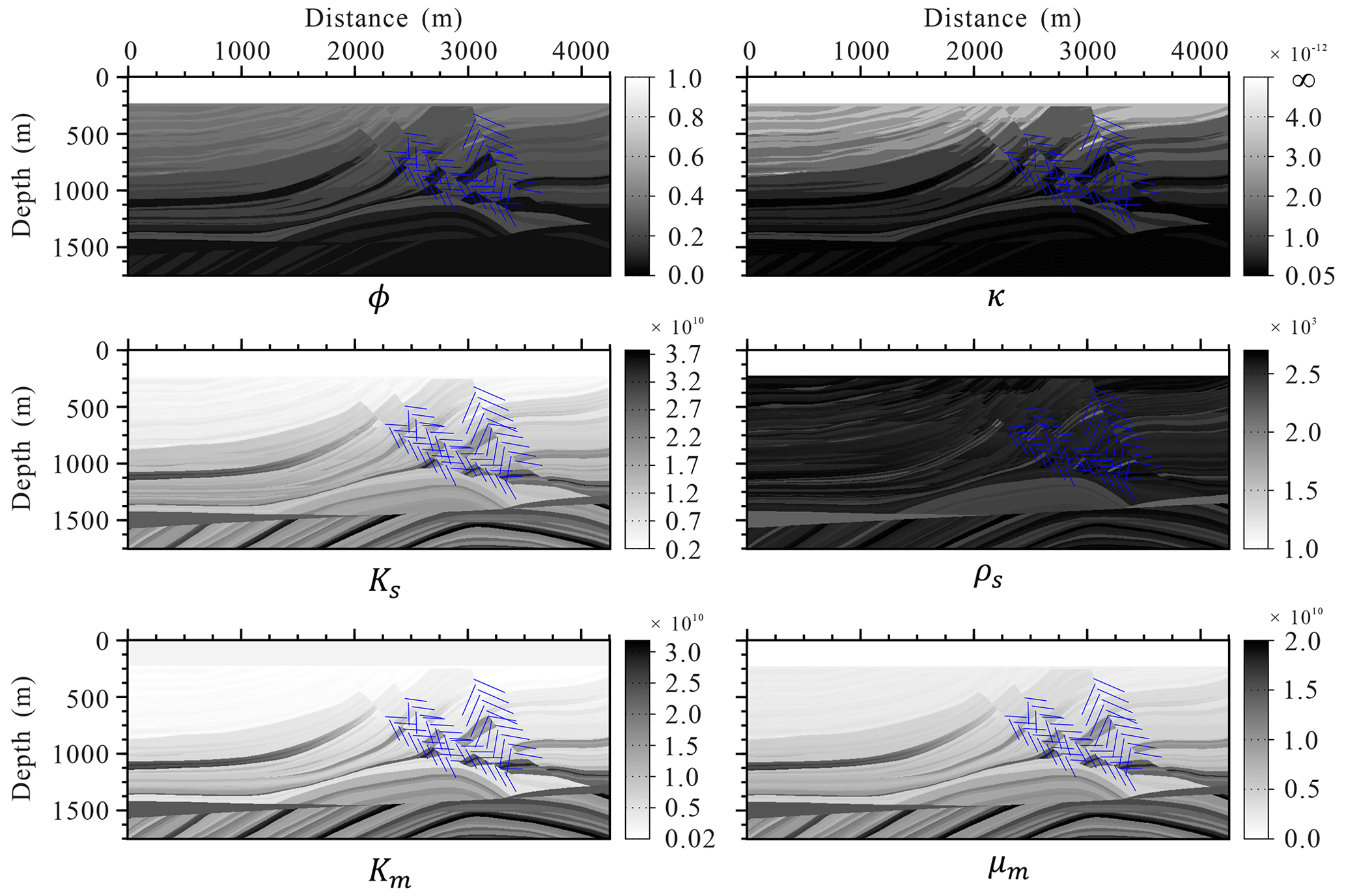
Figure 17 shows the snapshots of displacement fields at 1000 ms. The figure clearly shows the scattered P and S waves by the discretely distributed large-scale fractures. The results with such a complex model clearly verify the numerical implementation and the code. We also calculate the seismograms of the displacement shown in Fig. 18. The seismograms obtained by our proposed modeling scheme present the scattered seismic waves by the discrete fractures.

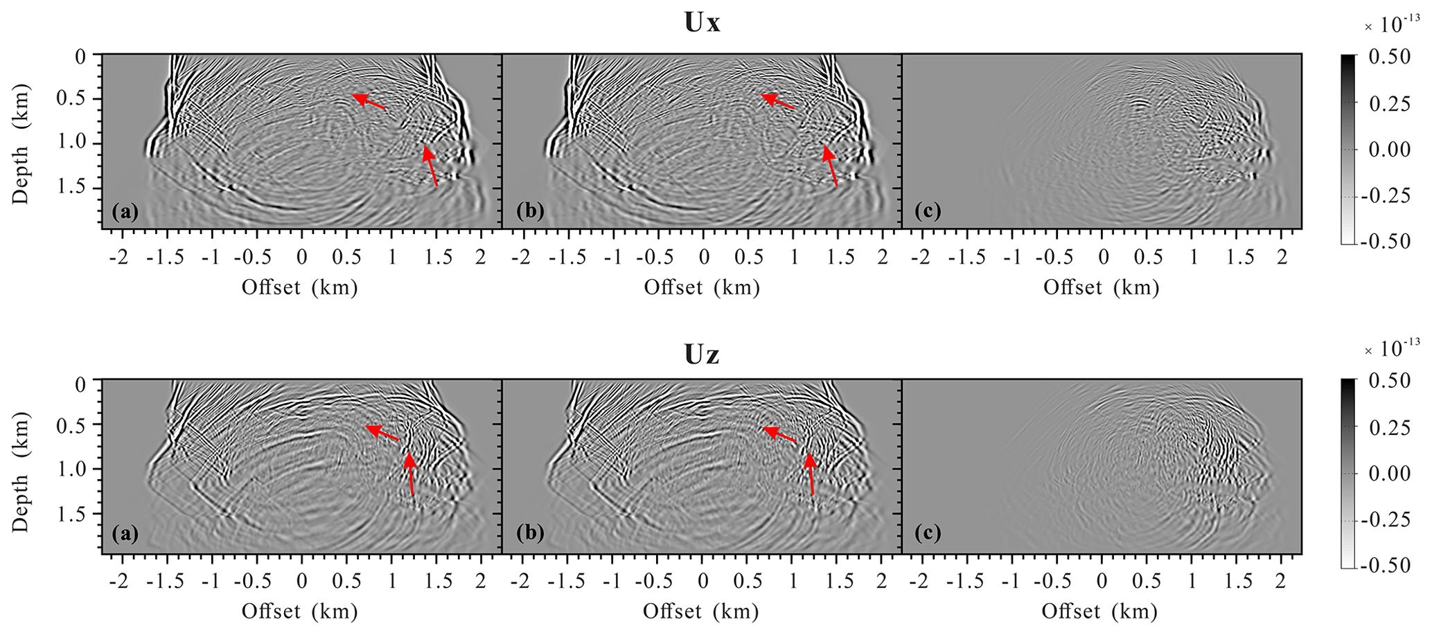
Figure 17 Snapshots of the wavefields components U_x and U_z at 1000 ms: (a) the original Marmousi model without fractures, (b) the modified Marmousi model with fractures, and (c) the differences.

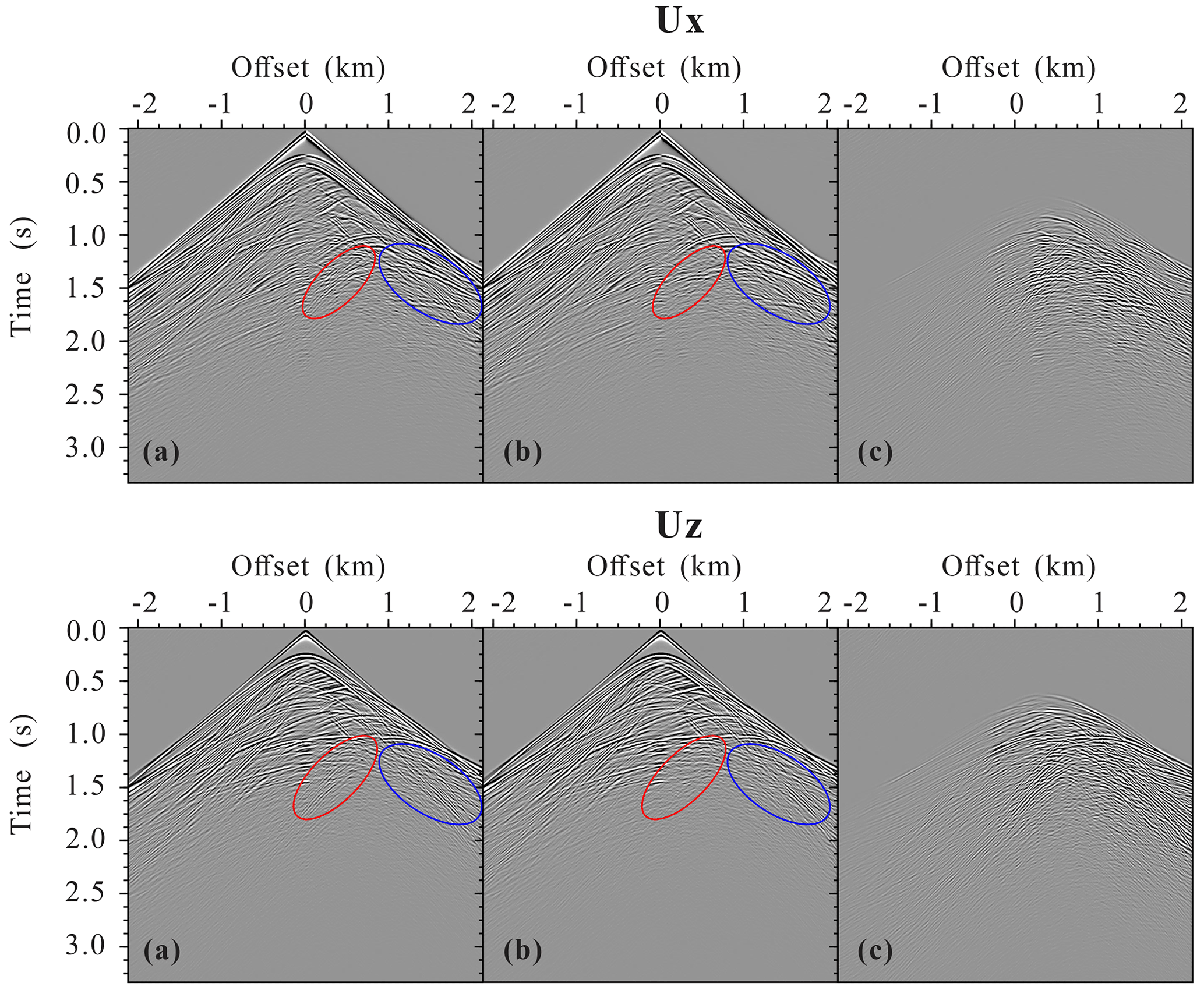
Figure 18 Seismogram components U_x and U_z: (a) the modified Marmousi model with fractures, (b) the original Marmousi model without fractures, and (c) the differences.

5 Conclusions

In this work, we have developed a numerical modeling scheme including FPD effects for discretely distributed large-scale fractures embedded in fluid-saturated porous rock. To capture the FPD effects between the fractures and background, the fractures are represented as Barbosa's VLSM with complex-valued and frequency-dependent fracture compliances. Using Coates and Schoenberg's local-effective-medium theory and Barbosa's VLSM, we derive the effective anisotropic viscoelastic compliances in each spatial discretized cell by superimposing the compliances of the background and the fractures. The effective governing equations of each numerical cell are expressed by the derived effective compliances and discretized by the mixed-grid-stencil FDFD method. The proposed modeling scheme can be used to study the impact of mechanical and hydraulic fracture properties on seismic scattering. The main advantage of our proposed modeling scheme over poroelastic modeling schemes is that the fractured domain can be modeled using a viscoelastic solid, while the rest of the domain can be modeled using an elastic solid.

The scattered P wave of a fluid-saturated horizontal fracture calculated by VLSM-based modeling is strongly affected by the FPD effects, while the scattered S wave is less sensitive, which is consistent with the result of PLSM-based modeling. However, the LVLSM-based modeling overestimates the scattered P wave and the HVLSM-based modeling underestimates the scattered P wave. The numerical results show that the proposed VLSM-based modeling can include the FPD effects and thus accurately estimate the scattered wave of the horizontal fracture. The results of the fractured reservoir models show that the amplitudes of the scattered waves from the top of the fractured reservoir are affected by the fluid stiffening effects due to the FPD effects. The scattered waves from the bottom of the fractured reservoir are also attenuated and dispersed by the FPD effects in addition to the fluid stiffening effects, and the reflected waves can retain the relevant attenuation and dispersion information. Randomly distributed fractures can also result in a different scattering characteristic than regularly distributed fractures; i.e., a large number of coda waves are generated due to increased inhomogeneity. The results of the modified Marmousi model clearly show the scattered waves by the discretely distributed large-scale fractures and verify the proposed numerical modeling scheme. The proposed numerical modeling scheme is expected not only to improve the estimations of seismic wave scattering from discretely distributed large-scale fractures but can also to improve migration quality and the estimation of fracture mechanical characteristics in inversion.

Appendix A: The coefficients related to spatial derivative operators

We define coefficient vectors ${\mathit{T}}_k\left(k=\mathrm{1},\mathrm{2},\mathrm{3},\mathrm{4}\right)$ and the derivative operate vector D(c) as

$$\begin{array}{}\text{(A1)}& {\displaystyle }\begin{array}{rl}& {\mathit{T}}_{\mathrm{1}}={\displaystyle \frac{\mathrm{1}}{{\mathit{\xi }}_x{\mathit{\xi }}_x}}\left[\mathrm{1}\mathrm{0}\mathrm{0}\mathrm{0}\right],{\mathit{T}}_{\mathrm{2}}={\displaystyle \frac{\mathrm{1}}{{\mathit{\xi }}_x{\mathit{\xi }}_z}}\left[\mathrm{0}\mathrm{1}\mathrm{0}\mathrm{0}\right],\\ & {\mathit{T}}_{\mathrm{3}}={\displaystyle \frac{\mathrm{1}}{{\mathit{\xi }}_x{\mathit{\xi }}_z}}\left[\mathrm{0}\mathrm{0}\mathrm{1}\mathrm{0}\right],{\mathit{T}}_{\mathrm{4}}={\displaystyle \frac{\mathrm{1}}{{\mathit{\xi }}_z{\mathit{\xi }}_z}}\left[\mathrm{0}\mathrm{0}\mathrm{0}\mathrm{1}\right],\end{array}\text{(A2)}& {\displaystyle }\mathit{D}\left(c\right)=\left[{\partial }_x\left(c{\partial }_x\right){\partial }_x\left(c{\partial }_z\right){\partial }_z\left(c{\partial }_x\right){\partial }_z\left(c{\partial }_z\right)\right],\end{array}$$

where ξ_x and ξ_z are the PML damping function and c represents effective stiffness. Then, the expression of A_c, B_c, C_c, D_c is written in matrix form:

$$\begin{array}{}\text{(A3)}& \left[\begin{array}{c}{A}_c\\ B_c\\ C_c\\ D_c\end{array}\right]=\left[\begin{array}{cccc}\mathit{D}\left(c_{\mathrm{11}}\right)& \mathit{D}\left(c_{\mathrm{15}}\right)& \mathit{D}\left(c_{\mathrm{15}}\right)& \mathit{D}\left(c_{\mathrm{55}}\right)\\ \mathit{D}\left(c_{\mathrm{15}}\right)& \mathit{D}\left(c_{\mathrm{55}}\right)& \mathit{D}\left(c_{\mathrm{13}}\right)& \mathit{D}\left(c_{\mathrm{35}}\right)\\ \mathit{D}\left(c_{\mathrm{15}}\right)& \mathit{D}\left(c_{\mathrm{13}}\right)& \mathit{D}\left(c_{\mathrm{55}}\right)& \mathit{D}\left(c_{\mathrm{35}}\right)\\ \mathit{D}\left(c_{\mathrm{55}}\right)& \mathit{D}\left(c_{\mathrm{35}}\right)& \mathit{D}\left(c_{\mathrm{35}}\right)& \mathit{D}\left(c_{\mathrm{33}}\right)\end{array}\right]\left[\begin{array}{c}{\mathit{T}}_{\mathrm{1}}\\ {\mathit{T}}_{\mathrm{2}}\\ {\mathit{T}}_{\mathrm{3}}\\ {\mathit{T}}_{\mathrm{4}}\end{array}\right].\end{array}$$

We formulate A_r, B_r, C_r, D_r in a similar way by defining the coefficient vectors ${{\mathit{T}}^{\prime }}_k\left(k=\mathrm{1},\mathrm{2},\mathrm{3},\mathrm{4}\right)$ and D^′(c) as

$$\begin{array}{}\text{(A4)}& {\displaystyle }\begin{array}{rl}& {{\mathit{T}}^{\prime }}_{\mathrm{1}}={\displaystyle \frac{\mathrm{1}}{\mathrm{2}{\mathit{\xi }}_x{\mathit{\xi }}_x}}\left[\mathrm{1}\mathrm{1}\mathrm{1}\mathrm{1}\right],{{\mathit{T}}^{\prime }}_{\mathrm{2}}={\displaystyle \frac{\mathrm{1}}{\mathrm{2}{\mathit{\xi }}_x{\mathit{\xi }}_z}}\left[-\mathrm{1}\mathrm{1}-\mathrm{1}\mathrm{1}\right],\\ & {{\mathit{T}}^{\prime }}_{\mathrm{3}}={\displaystyle \frac{\mathrm{1}}{\mathrm{2}{\mathit{\xi }}_x{\mathit{\xi }}_z}}\left[-\mathrm{1}-\mathrm{1}\mathrm{1}\mathrm{1}\right],{{\mathit{T}}^{\prime }}_{\mathrm{4}}={\displaystyle \frac{\mathrm{1}}{\mathrm{2}{\mathit{\xi }}_z{\mathit{\xi }}_z}}\left[\mathrm{1}-\mathrm{1}-\mathrm{1}\mathrm{1}\right],\end{array}\text{(A5)}& {\displaystyle }{\mathit{D}}^{\prime }\left(c\right)=\left[{\partial }_{x^{\prime }}\left(c{\partial }_{x^{\prime }}\right){\partial }_{x^{\prime }}\left(c{\partial }_{z^{\prime }}\right){\partial }_{z^{\prime }}\left(c{\partial }_{x^{\prime }}\right){\partial }_{z^{\prime }}\left(c{\partial }_{z^{\prime }}\right)\right].\end{array}$$

The expression of A_r, B_r, C_r, D_r is written as

$$\begin{array}{}\text{(A6)}& \left[\begin{array}{c}{A}_r\\ B_r\\ C_r\\ D_r\end{array}\right]=\left[\begin{array}{cccc}{\mathit{D}}^{\prime }\left(c_{\mathrm{11}}\right)& {\mathit{D}}^{\prime }\left(c_{\mathrm{15}}\right)& {\mathit{D}}^{\prime }\left(c_{\mathrm{15}}\right)& {\mathit{D}}^{\prime }\left(c_{\mathrm{55}}\right)\\ {\mathit{D}}^{\prime }\left(c_{\mathrm{15}}\right)& {\mathit{D}}^{\prime }\left(c_{\mathrm{55}}\right)& {\mathit{D}}^{\prime }\left(c_{\mathrm{13}}\right)& {\mathit{D}}^{\prime }\left(c_{\mathrm{35}}\right)\\ {\mathit{D}}^{\prime }\left(c_{\mathrm{15}}\right)& {\mathit{D}}^{\prime }\left(c_{\mathrm{13}}\right)& {\mathit{D}}^{\prime }\left(c_{\mathrm{55}}\right)& {\mathit{D}}^{\prime }\left(c_{\mathrm{35}}\right)\\ {\mathit{D}}^{\prime }\left(c_{\mathrm{55}}\right)& {\mathit{D}}^{\prime }\left(c_{\mathrm{35}}\right)& {\mathit{D}}^{\prime }\left(c_{\mathrm{35}}\right)& {\mathit{D}}^{\prime }\left(c_{\mathrm{33}}\right)\end{array}\right]\left[\begin{array}{c}{{\mathit{T}}^{\prime }}_{\mathrm{1}}\\ {{\mathit{T}}^{\prime }}_{\mathrm{2}}\\ {{\mathit{T}}^{\prime }}_{\mathrm{3}}\\ {{\mathit{T}}^{\prime }}_{\mathrm{4}}\end{array}\right].\end{array}$$

Appendix B: Parsimonious staggered-grid stencil

The nine coefficients of the CS stencil for the submatrix A_c of Eq. (27) are

$$\begin{array}{}\text{(B1)}& \begin{array}{rl}& A_{ci+\mathrm{1},j}={\displaystyle \frac{c_{\mathrm{11}i+\mathrm{0.5},j}}{{\mathrm{\Delta }}^{\mathrm{2}}{\mathit{\xi }}_{xi}{\mathit{\xi }}_{xi+\mathrm{0.5}}}},A_{ci-\mathrm{1},j}={\displaystyle \frac{c_{\mathrm{11}i-\mathrm{0.5},j}}{{\mathrm{\Delta }}^{\mathrm{2}}{\mathit{\xi }}_{xi}{\mathit{\xi }}_{xi-\mathrm{0.5}}}},\\ & A_{ci,j+\mathrm{1}}={\displaystyle \frac{c_{\mathrm{55}i,j+\mathrm{0.5}}}{{\mathrm{\Delta }}^{\mathrm{2}}{\mathit{\xi }}_{z\mathrm{j}}{\mathit{\xi }}_{zj+\mathrm{0.5}}}},A_{ci,j-\mathrm{1}}={\displaystyle \frac{c_{\mathrm{55}i,j-\mathrm{0.5}}}{{\mathrm{\Delta }}^{\mathrm{2}}{\mathit{\xi }}_{z\mathrm{j}}{\mathit{\xi }}_{zj-\mathrm{0.5}}}},\\ & A_{ci,j}=-{\displaystyle \frac{c_{\mathrm{11}i+\mathrm{0.5},j}}{{\mathrm{\Delta }}^{\mathrm{2}}{\mathit{\xi }}_{xi}{\mathit{\xi }}_{xi+\mathrm{0.5}}}}-{\displaystyle \frac{c_{\mathrm{11}i-\mathrm{0.5},j}}{{\mathrm{\Delta }}^{\mathrm{2}}{\mathit{\xi }}_{xi}{\mathit{\xi }}_{xi-\mathrm{0.5}}}}\\ & -{\displaystyle \frac{c_{\mathrm{55}i,j+\mathrm{0.5}}}{{\mathrm{\Delta }}^{\mathrm{2}}{\mathit{\xi }}_{zj}{\mathit{\xi }}_{zj+\mathrm{0.5}}}}-{\displaystyle \frac{c_{\mathrm{55}i,j-\mathrm{0.5}}}{{\mathrm{\Delta }}^{\mathrm{2}}{\mathit{\xi }}_{zj}{\mathit{\xi }}_{zj-\mathrm{0.5}}}},\\ & A_{ci+\mathrm{1},j+\mathrm{1}}={\displaystyle \frac{c_{\mathrm{15}i+\mathrm{1},j}+c_{\mathrm{15}i,j+\mathrm{1}}}{\mathrm{4}{\mathrm{\Delta }}^{\mathrm{2}}{\mathit{\xi }}_{xi}{\mathit{\xi }}_{zj}}},\\ & A_{ci+\mathrm{1},j-\mathrm{1}}=-{\displaystyle \frac{c_{\mathrm{15}i+\mathrm{1},j}+c_{\mathrm{15}i,j-\mathrm{1}}}{\mathrm{4}{\mathrm{\Delta }}^{\mathrm{2}}{\mathit{\xi }}_{xi}{\mathit{\xi }}_{zj}}},\\ & A_{ci-\mathrm{1},j+\mathrm{1}}=-{\displaystyle \frac{c_{\mathrm{15}i-\mathrm{1},j}+c_{\mathrm{15}i,j+\mathrm{1}}}{\mathrm{4}{\mathrm{\Delta }}^{\mathrm{2}}{\mathit{\xi }}_{xi}{\mathit{\xi }}_{zj}}},\\ & A_{ci-\mathrm{1},j-\mathrm{1}}={\displaystyle \frac{c_{\mathrm{15}i-\mathrm{1},j}+c_{\mathrm{15}i,j-\mathrm{1}}}{\mathrm{4}{\mathrm{\Delta }}^{\mathrm{2}}{\mathit{\xi }}_{xi}{\mathit{\xi }}_{zj}}}.\end{array}\end{array}$$

The nine coefficients of the RS stencil for the submatrix A_r of Eq. (27) are

$$\begin{array}{}\text{(B2)}& \begin{array}{rl}& A_{ri+\mathrm{1},j}={\displaystyle \frac{c_{\mathrm{11}i+\mathrm{0.5},j-\mathrm{0.5}}-c_{\mathrm{55}i+\mathrm{0.5},j-\mathrm{0.5}}}{\mathrm{4}{\mathrm{\Delta }}^{\mathrm{2}}{\mathit{\xi }}_{xi}{\mathit{\xi }}_{zj-\mathrm{0.5}}}}\\ & +{\displaystyle \frac{c_{\mathrm{11}i+\mathrm{0.5},j+\mathrm{0.5}}-c_{\mathrm{55}i+\mathrm{0.5},j+\mathrm{0.5}}}{\mathrm{4}{\mathrm{\Delta }}^{\mathrm{2}}{\mathit{\xi }}_{zj}{\mathit{\xi }}_{xi+\mathrm{0.5}}}},\\ & A_{ri-\mathrm{1},j}={\displaystyle \frac{c_{\mathrm{11}i-\mathrm{0.5},j+\mathrm{0.5}}-c_{\mathrm{55}i-\mathrm{0.5},j+\mathrm{0.5}}}{\mathrm{4}{\mathrm{\Delta }}^{\mathrm{2}}{\mathit{\xi }}_{xi}{\mathit{\xi }}_{zj+\mathrm{0.5}}}}\\ & +{\displaystyle \frac{c_{\mathrm{11}i-\mathrm{0.5},j-\mathrm{0.5}}-c_{\mathrm{55}i-\mathrm{0.5},j-\mathrm{0.5}}}{\mathrm{4}{\mathrm{\Delta }}^{\mathrm{2}}{\mathit{\xi }}_{zj}{\mathit{\xi }}_{xi-\mathrm{0.5}}}},\\ & A_{ri,j+\mathrm{1}}={\displaystyle \frac{c_{\mathrm{55}i-\mathrm{0.5},j+\mathrm{0.5}}-c_{\mathrm{11}i-\mathrm{0.5},j+\mathrm{0.5}}}{\mathrm{4}{\mathrm{\Delta }}^{\mathrm{2}}{\mathit{\xi }}_{xi}{\mathit{\xi }}_{zj+\mathrm{0.5}}}}\\ & +{\displaystyle \frac{c_{\mathrm{55}i+\mathrm{0.5},j+\mathrm{0.5}}-c_{\mathrm{11}i+\mathrm{0.5},j+\mathrm{0.5}}}{\mathrm{4}{\mathrm{\Delta }}^{\mathrm{2}}{\mathit{\xi }}_{zj}{\mathit{\xi }}_{xi+\mathrm{0.5}}}},\\ & A_{ri,j-\mathrm{1}}={\displaystyle \frac{c_{\mathrm{55}i+\mathrm{0.5},j-\mathrm{0.5}}-c_{\mathrm{11}i+\mathrm{0.5},j-\mathrm{0.5}}}{\mathrm{4}{\mathrm{\Delta }}^{\mathrm{2}}{\mathit{\xi }}_{xi}{\mathit{\xi }}_{zj-\mathrm{0.5}}}}\\ & +{\displaystyle \frac{c_{\mathrm{55}i-\mathrm{0.5},j-\mathrm{0.5}}-c_{\mathrm{11}i-\mathrm{0.5},j-\mathrm{0.5}}}{\mathrm{4}{\mathrm{\Delta }}^{\mathrm{2}}{\mathit{\xi }}_{zj}{\mathit{\xi }}_{xi-\mathrm{0.5}}}},\\ & A_{ri,j}=-{\displaystyle \frac{c_{\mathrm{11}i+\mathrm{0.5},j-\mathrm{0.5}}-\mathrm{2}{c}_{\mathrm{15}i+\mathrm{0.5},j-\mathrm{0.5}}+c_{\mathrm{55}i+\mathrm{0.5},j-\mathrm{0.5}}}{\mathrm{4}{\mathrm{\Delta }}^{\mathrm{2}}{\mathit{\xi }}_{xi}{\mathit{\xi }}_{xi+\mathrm{0.5}}}}\\ & -{\displaystyle \frac{c_{\mathrm{11}i-\mathrm{0.5},j+\mathrm{0.5}}-\mathrm{2}{c}_{\mathrm{15}i-\mathrm{0.5},j+\mathrm{0.5}}+c_{\mathrm{55}i-\mathrm{0.5},j+\mathrm{0.5}}}{\mathrm{4}{\mathrm{\Delta }}^{\mathrm{2}}{\mathit{\xi }}_{xi}{\mathit{\xi }}_{xi-\mathrm{0.5}}}}\\ & -{\displaystyle \frac{c_{\mathrm{11}i+\mathrm{0.5},j+\mathrm{0.5}}+\mathrm{2}{c}_{\mathrm{15}i+\mathrm{0.5},j+\mathrm{0.5}}+c_{\mathrm{55}i+\mathrm{0.5},j+\mathrm{0.5}}}{\mathrm{4}{\mathrm{\Delta }}^{\mathrm{2}}{\mathit{\xi }}_{zj}{\mathit{\xi }}_{zj+\mathrm{0.5}}}}\\ & -{\displaystyle \frac{c_{\mathrm{11}i-\mathrm{0.5},j-\mathrm{0.5}}+\mathrm{2}{c}_{\mathrm{15}i-\mathrm{0.5},j-\mathrm{0.5}}+c_{\mathrm{55}i-\mathrm{0.5},j-\mathrm{0.5}}}{\mathrm{4}{\mathrm{\Delta }}^{\mathrm{2}}{\mathit{\xi }}_{zj}{\mathit{\xi }}_{zj-\mathrm{0.5}}}}\\ & A_{ri+\mathrm{1},j+\mathrm{1}}={\displaystyle \frac{c_{\mathrm{11}i+\mathrm{0.5},j+\mathrm{0.5}}+\mathrm{2}{c}_{\mathrm{15}i+\mathrm{0.5},j+\mathrm{0.5}}+c_{\mathrm{55}i+\mathrm{0.5},j+\mathrm{0.5}}}{\mathrm{4}{\mathrm{\Delta }}^{\mathrm{2}}{\mathit{\xi }}_{zj}{\mathit{\xi }}_{zj+\mathrm{0.5}}}},\\ & A_{ri+\mathrm{1},j-\mathrm{1}}={\displaystyle \frac{c_{\mathrm{11}i+\mathrm{0.5},j-\mathrm{0.5}}-\mathrm{2}{c}_{\mathrm{15}i+\mathrm{0.5},j-\mathrm{0.5}}+c_{\mathrm{55}i+\mathrm{0.5},j-\mathrm{0.5}}}{\mathrm{4}{\mathrm{\Delta }}^{\mathrm{2}}{\mathit{\xi }}_{xi}{\mathit{\xi }}_{xi+\mathrm{0.5}}}},\\ & A_{ri-\mathrm{1},j+\mathrm{1}}={\displaystyle \frac{c_{\mathrm{11}i-\mathrm{0.5},j+\mathrm{0.5}}-\mathrm{2}{c}_{\mathrm{15}i-\mathrm{0.5},j+\mathrm{0.5}}+c_{\mathrm{55}i-\mathrm{0.5},j+\mathrm{0.5}}}{\mathrm{4}{\mathrm{\Delta }}^{\mathrm{2}}{\mathit{\xi }}_{xi}{\mathit{\xi }}_{xi-\mathrm{0.5}}}},\\ & A_{ri-\mathrm{1},j-\mathrm{1}}={\displaystyle \frac{c_{\mathrm{11}i-\mathrm{0.5},j-\mathrm{0.5}}+\mathrm{2}{c}_{\mathrm{15}i-\mathrm{0.5},j-\mathrm{0.5}}+c_{\mathrm{55}i-\mathrm{0.5},j-\mathrm{0.5}}}{\mathrm{4}{\mathrm{\Delta }}^{\mathrm{2}}{\mathit{\xi }}_{zj}{\mathit{\xi }}_{zj-\mathrm{0.5}}}}.\end{array}\end{array}$$

The coefficients of the submatrices B_c, C_c, D_c and B_r, C_r, D_r can be inferred easily from those of submatrix A_c and A_r, respectively.