the Creative Commons Attribution 4.0 License.
the Creative Commons Attribution 4.0 License.
 | 02 Feb 2024
Integration of automatic implicit geological modelling in deterministic geophysical inversion
Jérémie Giraud
Guillaume Caumon
Lachlan Grose
Vitaliy Ogarko
Paul Cupillard
We propose and evaluate methods for the integration of automatic implicit geological modelling into the geophysical (potential field) inversion process. The objective is to enforce structural geological realism and to consider geological observations in a level set inversion, which inverts for the location of the boundaries between rock units. We propose two approaches. In the first approach, a geological correction term is applied at each iteration of the inversion to reduce geological inconsistencies. This is achieved by integrating an automatic implicit geological modelling scheme within the geophysical inversion process. In the second approach, we use automatic geological modelling to derive a dynamic prior model term at each iteration of the inversion to limit departures from geologically feasible outcomes. We introduce the main theoretical aspects of the inversion algorithm and perform the proof of concept using two synthetic studies. The analysis of the results using indicators measuring geophysical, petrophysical, and structural geological misfits demonstrates that our approach effectively steers the inversion towards geologically consistent models and reduces the risk of geologically unrealistic outcomes. Results suggest that the geological correction may be effectively applied to pre-existing geophysical models to increase their geological realism and that it can also be used to explore geophysically equivalent models.
- Article
(12339 KB) - Full-text XML
-
Supplement
(677 KB) - BibTeX
- EndNote


One of the long-standing challenges faced by geophysical inversion in general, and potential field studies in particular, is the recovery of geologically meaningful inverse models. One of the chief factors explaining this is the strong non-uniqueness of the solution to the inverse problem because an infinite number of models can fit a given potential field dataset, thereby allowing a wide range of geologically unrealistic outcomes. This has prompted the development of a number of approaches using prior information or constraints during inversion that aim at limiting the search space to models fitting the geophysical measurements (see, e.g., Lelièvre and Farquharson, 2016; Moorkamp, 2017; Wellmann and Caumon, 2018; Giraud et al., 2021b, and references therein). Earlier proposals comprise the use and design of regularisation schemes that account for prior information about the spatial variations in the inverted properties (e.g. smoothness constraints; Li and Oldenburg, 1996) or are a departure from a reference model based on some hypothesis (e.g. smallness constraints; Hoerl and Kennard, 1970). A more recent, and drastic, approach to reducing the size of the search space is to consider the geometry of the contact between rock units instead of the distribution of petrophysical values. In such a case, the physical properties of the rock units are assumed to be known a priori and can be kept constant during inversion. This idea was proposed decades ago for ray-based inversion in reflection seismology (Gjoystdal et al., 1985), but it raises challenges regarding the automatic maintenance of consistent relationships between geological interfaces (Caumon et al., 2004). More recently, surface-based inversion has become practical for seismic or for potential field inversion by using either an explicit formulation for the interface between rock units (Galley et al., 2020, 2021) or using level sets in the inversion (e.g. Dahlke et al., 2020; Giraud et al., 2021a; Li et al., 2017, 2020; Rashidifard et al., 2021; Zheglova et al., 2018, 2013). In the implicit boundary representation, the unit boundaries correspond to the zero iso value of the implicit functions representing the signed distance to the interfaces. In this type of modelling, the algorithms invert directly for the location of the contacts between the geological units by adjusting the location of these level sets, thereby allowing the automatic deformation of the geological units using geophysical data. Implicit formulations have a better ability than explicit surfaces to maintain the volumetric validity throughout model updates and can additionally deal with topological changes (Collon et al., 2016; Wellmann and Caumon, 2018).
In exploration geophysics, recent studies have applied level set inversion to the recovery of the geometry of one or two anomalous units in both single-physics or multi-physics inversions (Zheglova et al., 2018; Li et al., 2016, 2017). Subsequent works comprise the extension and modification of level set inversion by Giraud et al. (2021a) and Rashidifard et al. (2021), whose framework addresses an arbitrary number of rock units in a 3D gravity inversion. In comparison to the direct inversion of physical properties (i.e. density, electrical resistivity, and seismic velocities), these geometrical inversions present a direct pathway to obtain geologically realistic outcomes from the inversion of potential field data. Nonetheless, to the best of our knowledge, level set inversions still lack the capability to ensure the geological plausibility of inverted models, in the sense that they can produce alterations of the original models that can potentially violate geological principles while exploring the geophysical data space. To mitigate this, several solutions may be devised. One possibility, explored recently by Güdük et al. (2021) and Liang et al. (2023), consists of computing the geophysical response directly on geological models. In what follows, we propose two alternative approaches for the integration of geophysical inversion and geological modelling that allow more freedom for the geophysical component of the workflow as a result of applying a geological correction either during or after the level-set-based geophysical inversion. In the first case, one can think of ensuring geological plausibility a posteriori using an ad hoc process in which an existing geophysical inverse model undergoes modifications until it satisfies the geological plausibility conditions. This could be applied, for instance, to existing rock unit models obtained from previous geophysical processing or interpretation. In the second case, there is the possibility of integrating geological modelling principles, data, and rules directly within the geophysical inversion algorithm. In this contribution, we will focus on, and explore, the following two avenues:
- a.
the application of geological correction to the proposed model at each iteration of the geophysical inversion to ensure that the search for a model honouring geophysical measurements does not decrease the geological realism (introduced in Sect. 3.3.1 and tested in Sect. 5.1 and 5.2); and
- b.
the incorporation of a geological term in the objective function of the geophysical inverse problem (introduced in Sect. 3.3.2 and tested in Sect. 5.2).
In the two points above, the recovery of geological parameters from models proposed during inversion is necessary. At each iteration of the inversion, geological quantities such as the orientation of a contact or its location are extracted from the current model and subsequently fed to a geological modelling engine. The geological modelling engine will, in turn, propose the geological realisation closest to the geophysical inverse model from which a “geological correction” can be calculated and applied to the model update. This forms the basis of geological correction (point (a.) above) and ensures that geological consistency with principles and data is maintained throughout inversion. The same principle is used in point (b.) but for the definition of a constraint term as part of the inversion's objective function.
The main objective of this contribution is to introduce the methodology allowing the integration of automated geological modelling in the geophysical inversion process, as mentioned above, and to provide idealised proofs of concept in the form of two synthetic examples. This paper is divided into six sections, as follows. In the second section, we introduce the inversion algorithm that we use to integrate geological constraints. Following this, in Sect. 3, we provide the elements of implicit geological modelling required by the automated geological modelling process used to constrain geophysical inversion. In this section, we also detail how the geological constraints are applied, using the approaches (a) and (b) mentioned above, through an automated geological modelling process. In Sect. 4, we introduce the series of metrics that we consider to assess inversion convergence and also the recovered models from both the geological and geophysical points of view. Section 5 presents the proof of concept, using two synthetic examples of 3D models representing idealised scenarios. In the Discussion (Sect. 6), we place our findings in the broader context of subsurface modelling, discuss the limitations and implications of our work, and review potential extensions of the proposed method.
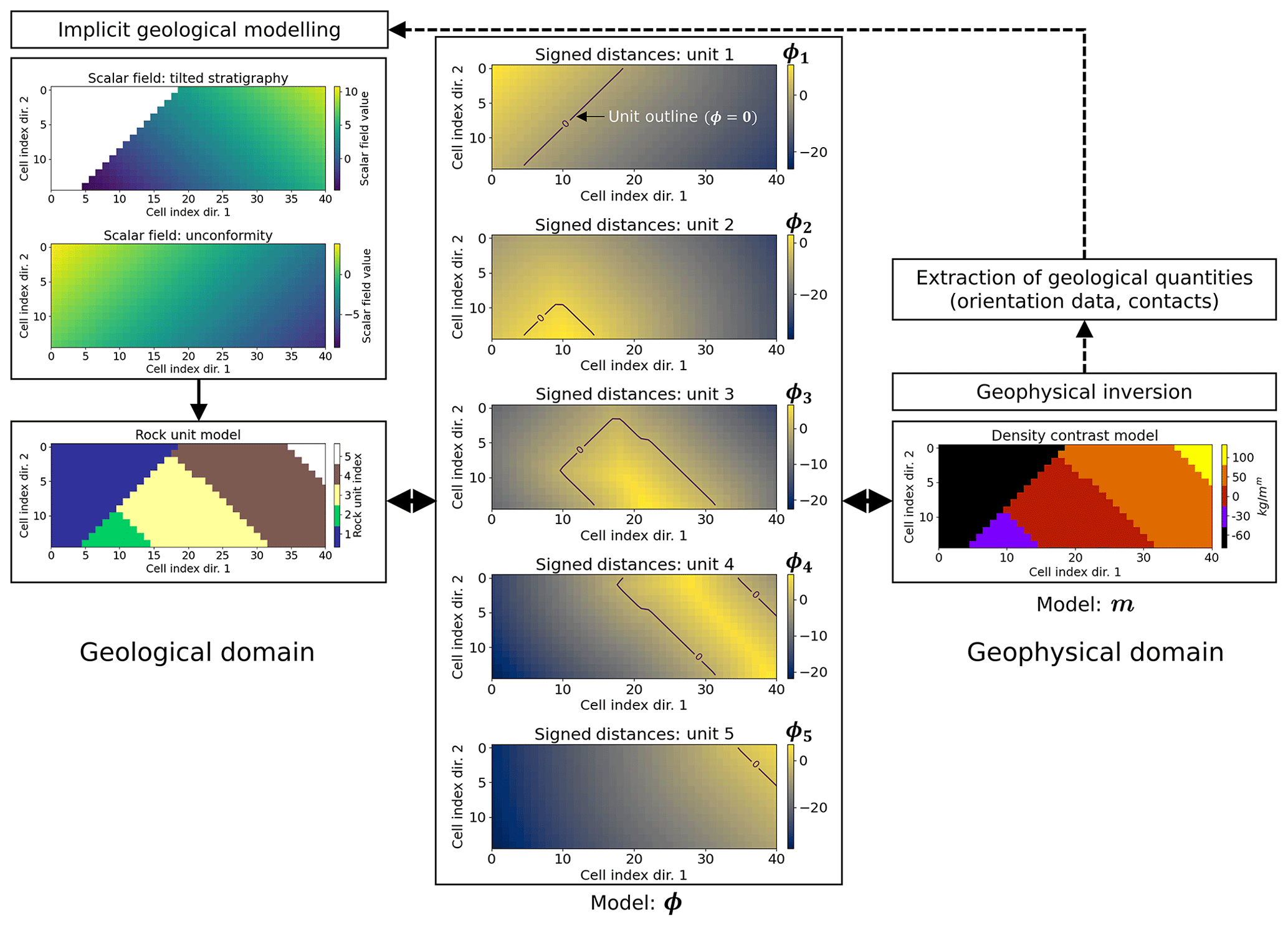
Figure 1Proposed strategy to link implicit geological modelling with geophysical level set inversion. The geological domain represents implicit geological modelling (left-hand side) and relates to Sect. 3.1 and 3.2. The middle and right-hand side panels illustrate the link between the signed distances and density contrasts introduced in Sect. 2.1. The dashed line with an arrow connecting the geophysical inversion to the geological domain symbolises the exchange of information between geological and geophysical modelling that can be used to link the two modelling processes.
2.1 Pre-requisite: linking rock unit boundaries to physical property inversion
The proposed method relies on the formulation of the model using an implicit model formulation in the form of signed distances to interfaces between rock units (right-hand side of Fig. 1). As proposed by Giraud et al. (2021a), this modelling approach considers rock units to be one or more rock types characterised by the same physical value (e.g. each unit is characterised by a single density value within the modelled area). Each rock unit is modelled by a unique signed-distance scalar field covering the study area. In a study considering nr rock units of known contrasting physical properties, we consider a set of nr signed-distance fields ϕ={ϕk, k=1, …, nr} over nm model cells corresponding to the distance to the boundaries of rock units. These signed distances are calculated using the fast-marching method of Sethian (1996) to maintain the following properties:
In our level set inversions, ϕ is the primary variable considered for inversion. It constitutes the proxy for a direct link that maps the geophysical and geological representations of the subsurface. We map these signed distances to petrophysical properties using
where is a vector storing the physical property value assigned to each of the nr geological units (e.g. density contrasts for the different rock units in the case of gravity inversion). Similar to Giraud et al. (2021a), H is the smeared-out Heaviside function, which is calculated following Osher and Fedkiw (2003). This smearing is useful for the calculation of the sensitivity matrix of the calculated data to changes in ϕ from Eq. (2). When adapting it to our problem, H is defined for the kth rock unit in the ith model cell as
where τ={τi, i=1, …, nm} defines the volume of rock at which the boundary is allowed to vary between two successive iterations of the inversion. To the best of our knowledge, it is common to set all τi values to a constant, equal to (Li et al., 2017), in a regular mesh of cells with a volume of . In our implementation, we extend this to the possibility of using spatially varying boundary thicknesses by allowing the neighbourhood defined by τ to vary in space. This enables the anchoring of the model at observation points where τi= 0, e.g. at surface observations, in boreholes, and along seismic lines. In extreme scenarios, the volume occupied by boundaries with of cells with a volume of may cover extensive parts of the study area or, conversely, prevent the model from evolving when τ=0 everywhere.
At each iteration of the inversion, m is updated from the changes in ϕ, δϕ, which are required by the process of optimising the objective function (also called the cost function; see Sect. 2.2) within the domain defined by non-null values of τ.
2.2 General formulation
We formulate the inverse problem in the least squares sense, taking gravity data inversion as an example. By adjusting the words of Giraud et al. (2021a), the choice of a least squares framework is motivated by the flexibility it allows in terms of the number of constraints and the forms of prior information that can be used in the inversion. Note that it corresponds to a maximum a posteriori estimator (Tarantola, 2005).
The objective function to minimise reads as follows:
where dobs is the observed data, and dcalc is the gravity response of the density contrast model m(ϕ). We use , where Sm is the sensitivity matrix of the gravity data d to changes in densities m(ϕ). The first term of Eq. (4) corresponds to a data misfit term, whereas the second term is a regularisation term that minimises deviations from the prior model. λp is a positive scalar weighting the regularisation term. Wp is an inverse diagonal variance matrix of dimensions (nmnr)×(nmnr), whose values can vary in space according to prior information to favour or discourage specific changes or features in the model. We note that the definition of Wp used here differs from Giraud et al. (2021a), where Wp is constituted of line vectors and has the dimensions nr×(nmnr). This allows for more flexibility when translating prior information into constraints on a cell-by-cell basis. ϕprior is the signed distances of a prior model. For simplicity, we do not include data measurement and modelling errors in the term of Eq. (4) but instead stop the inversion when the solution reaches a prescribed misfit level. Naturally, variable measurement errors could be integrated by replacing this term by the more general expression , where Cd would be the data covariance matrix.
We solve Eq. (4) iteratively and calculate the update of the signed distances δϕk that reduces Ψ(ϕk,dobs) at each iteration k. To solve for δϕk, we build the system of equations given in Appendix A, which requires the sensitivity matrix Sϕ,k of dcalc(m(ϕk)) with respect to changes in ϕk, using the chain rule:
where is obtained analytically from Eqs. (2) and (3) (see Giraud et al., 2021a, for details).
It can be shown that the objective function Ψ(ϕ,dobs) is equal to the log-posterior probability density distribution, as formulated in the Bayesian framework (Tarantola, 2005; see their Chapters 1 and 3 for more details). Here, the problem is therefore cast as a maximum a posteriori estimation. At the kth iteration, we calculate ϕk+1, such that and the updated model m(ϕk+1) is calculated consistently with Eq. (2) by selecting the rock unit with the largest signed-distance value at each model cell i=1, …, nm.
We remind the reader that the vector contains the physical property values assigned to the different geological units (see Eq. 2). In Eq. (6), the argmax function leads to the selection of the density contrast corresponding to the highest value of ϕ, which, intuitively, corresponds to the “innermost” rock unit. Following the same rationale as Zheglova et al. (2013), we then calculate the signed distances corresponding to the updated boundaries of mk+1 to maintain the signed-distance properties of ϕk+1, as introduced in Sect. 2.1. We note that at any given iteration, the search space is restricted to the vicinity of boundaries between rock units, as defined by the boundary's neighbourhood controlled by τ, which determines the current inversion's domain. This localisation dramatically reduces the volume of rock and the number of model cells considered for modification between two successive iterations to satisfy geophysical data fit requirements.
2.3 Prior model constraints on signed distances
Using a prior structural geological model, the corresponding signed distances ϕprior to boundaries can be calculated. We remind the reader that in Eq. (4), the prior model constraints on signed distances are given as .
This allows the inversion to explore the part of the model space remaining within the neighbourhood of ϕprior. The size of this neighbourhood globally depends on λp, which controls the relative importance assigned to the prior model term during inversion compared to the geophysical data misfit term. It is also locally determined by Wp, which tunes the importance of the prior model term for each model cell. Similar to other least squares inversions, λp can be set manually by trial and error, for example, by starting with a high value that will be reduced until model changes occur. Alternatively, the L-curve (Hansen and Johnston, 2001; Hansen and O'Leary, 1993) or general cross-validation principle (Farquharson and Oldenburg, 2004) may be used. In instances where a geological prior model is used, it is generally obtained before geophysical inversion and remains constant throughout inversion. In this contribution, our objective is to use, as a prior model, the result of a geological modelling process anchored only to the geological data and principles to better explore the admissible geological and geophysical parameter space.
The goal of this section is to introduce possible methods for extracting geological information in the form of the contact location and orientation data (angles) of geological features from inverted models that can be subsequently treated as geological data to implicit geological modelling.
3.1 Pre-requisite: implicit geological modelling in a nutshell
In implicit modelling, geological structures (e.g. faults, foliations, intrusions, and stratigraphic horizons) are represented by iso values of one or several 3D scalar fields (see Wellmann and Caumon, 2018, for a review). For example, fault surfaces are generated as iso values of signed-distance functions (possibly restricted to a given region of space), and strata are generated as iso values of a relative geological time function. For each geological surface or series of surfaces, the 3D scalar field is obtained by least squares interpolation between the spatial measurement points. In this paper, we use LoopStructural, which is an open-source Python library for implicit 3D geological modelling (Grose et al., 2021). In LoopStructural, geological features are modelled backwards in time, starting with the most recent. Faults are modelled by first modelling the fault surface and fault displacement vector by building a structural frame consisting of three signed-distance fields representing the fault geometry and kinematics. The fault can then be applied to the faulted features by restoring the observations of the faulted surface prior to interpolating the faulted surface. This means that the kinematics of the fault are directly incorporated into the surface description.
LoopStructural uses a discrete implicit modelling approach, where the implicit function is approximated using a piecewise combination of basis functions on a predefined support, such as a linear tetrahedron on a tetrahedral mesh or a trilinear basis function on a Cartesian grid. Discrete implicit modelling forms an under-constrained system of equations because geological observations are sparse, and there are usually more degrees of freedom than geological constraints (location or orientation of geological features). To ensure the stability of the solution, a continuous regularisation term is added. Usual choices for regularisation constraints are some type of discrete smoothness constraint (Frank et al., 2007; Irakarama et al., 2021) or the minimisation of a continuous energy (Irakarama et al., 2022; Renaudeau et al., 2019). In this study, we use the finite difference regularisation, as implemented in LoopStructural, which minimises the second derivative of the scalar fields in all directions, using a finite difference scheme on a Cartesian grid (following Irakarama et al., 2021).
Geological observations such as the location of contacts, form lines, fault locations, and structural measurements can constrain the value and/or the gradient of the implicit function (Frank et al., 2007). Geological observations (further denoted as dgeol) are incorporated by finding the mesh element which contains the observation point and adding the linear constraint for the relevant degrees of freedom (nodes of the element). Orientation data can be used to constrain the gradient of the implicit function g as follows:
where n is the normal vector of the geological surface at the location x. As Eq. (7) constrains both the direction and magnitude of the gradient of the scalar field, an alternative formulation, used to impose only the orientation, is to find two tangent vectors, e.g. the strike vector vstrike and dip vector vdip, and to set the following:
Geological contacts or the location of geological features are integrated into the implicit modelling by setting the value of the implicit function as follows:
where val is the value of the implicit function given at the location x. The value should represent the distance to a reference horizon (for example, zero when the observation is located directly on the surface, such as a fault surface, being modelled) or the cumulative stratigraphic thickness to some reference horizon for different conforming stratigraphic interfaces. The implicit function is determined by solving the resulting regularised, overdetermined problem using least squares minimisation. For this reason, LoopStructural uses a conjugate gradient algorithm to iteratively find the solution of the system of equations.
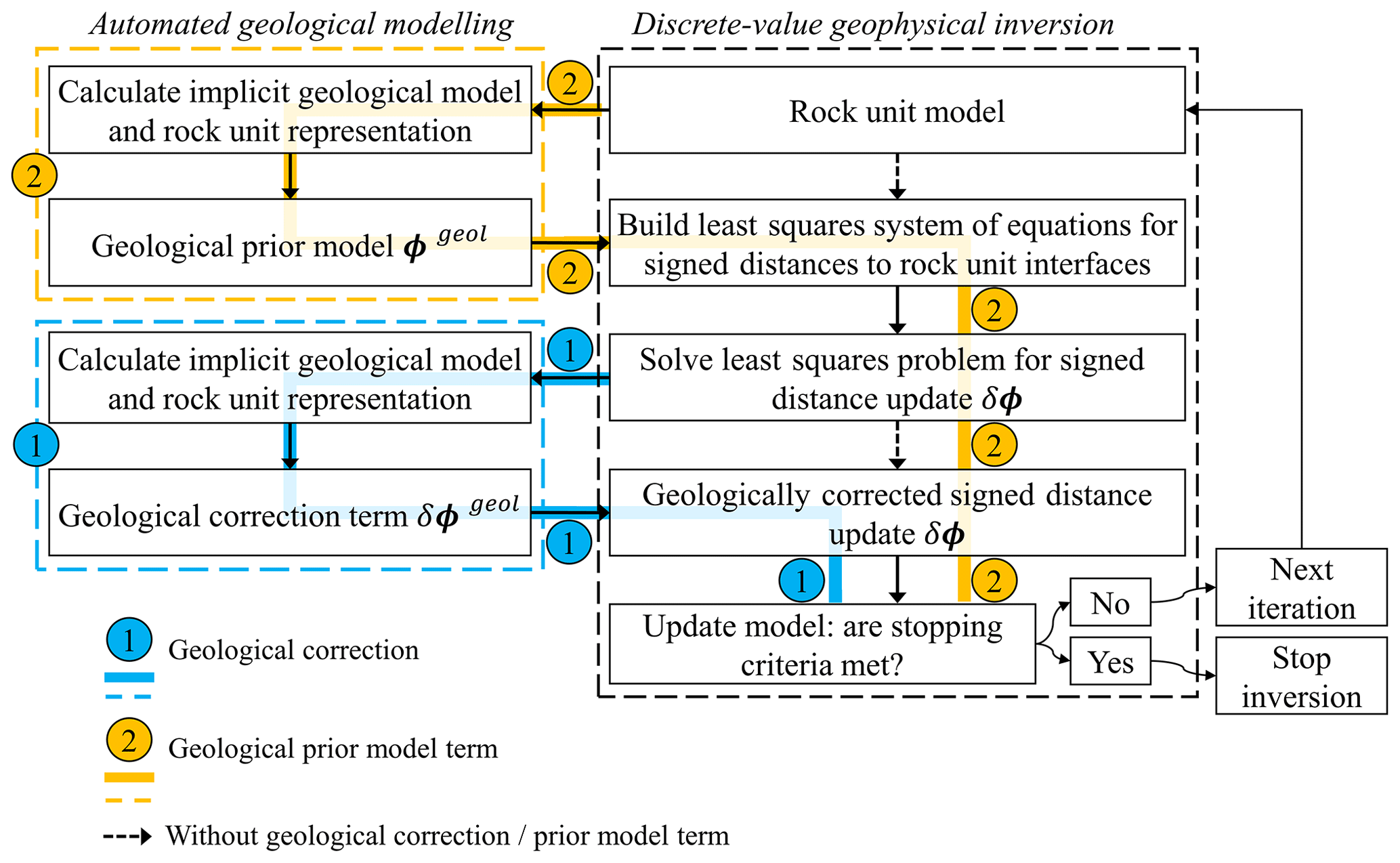
Figure 2Summary of the proposed approaches to the integration of geological modelling in geophysical inversion with the iterative use of the geological correction term with a fixed prior (1) or an update of the prior geological model (2). Note that the combination of both is possible. This flowchart has been modified from Giraud et al. (2022).
In the next few subsections, we introduce how to recover input data for implicit geological modelling, as mentioned above, from models obtained through geophysical inversion. More specifically, we detail how to
-
extract the location of contacts between units from geophysical regions to constrain stratigraphic contacts; and
-
retrieve orientation data from the plane approximating the location of the contacts between non-conformable units to model an unconformity using both geological and geophysical modelling.
We note that while we use LoopStructural, the generation of geological models using the data provided in this paper can be carried out with other implicit geological modelling engines, such as through the GeoModeller application programming interface (Calcagno et al., 2008; Guillen et al., 2008), GemPy (De La Varga et al., 2019), SKUA-GOCAD (Jayr et al., 2008), Petrel (Souche et al., 2015), or Leapfrog Geo software (Cowan and Beatson, 2002).
3.2 Recovering structural information from and for geophysical inversion
3.2.1 Stratigraphic information
In implicit geological modelling, interfaces are defined by iso values of one or several scalar fields analogous to signed distances or to relative geological time. This opens up pathways to integrate implicit geological modelling and level set inversion as introduced above and illustrated in Fig. 2. Stratigraphic information are recovered from the current geophysical model by identification of the contacts between rock units. More specifically, the 3D coordinates of the top of the different units within a given layered stratigraphy are extracted from 3D rock unit models and stored as input data (as in Eq. 9) for implicit geological modelling.
3.2.2 Orientation observations: example of a subplanar unconformity
In some cases, interpretive orientation data can be used as input to geological modelling (e.g. Sprague and de Kemp, 2005). Similarly, the geophysical level set approach provides region boundary orientation, which can be used to locally constrain the planar orientations of geological interfaces.
For instance, let us consider the example of a roughly planar erosion surface affecting some older stratigraphic series which constitute an unconformity. We propose recovering the average normal vector n to this plane, which is required for the implicit model to be well posed in the absence of post-erosional stratigraphic data, by the
-
identification of the contact locations for the surface of interest from the current geophysical model ϕ; and
-
calculation of the best-fitting plane approximating the identified locations of the selected contacts (constrained least squares fit through a least squares minimisation process; see Appendix B).
After it is recovered, the vector n is normalised and used with Eqs. (7) or (8) in implicit geological modelling.
3.3 Automated geological modelling during inversion
3.3.1 Geological correction
A way to promote geological consistency at each iteration of the geophysical inversion is to adjust the model update δϕ to limit changes in ϕ that contradict the geological data and principles. For this, we apply what we further refer to as a “geological correction term” to the update term δϕ, which is obtained from solving Eq. (4). In what follows, we introduce the “geological” signed distances or relative geological time values fgeol to the rock units corresponding to the geological model derived from the geological data dgeol and the current geophysical update of ϕ. fgeol can be seen as a re-parameterisation of the geological model in a way that is compatible with the geophysical signed-distance values ϕ. In other words, the application of fgeol consists of the calculation of the geological image of the geophysical signed-distance values ϕ. It is computed using the following:
-
extraction of geological information from the current signed-distance model (with contacts and orientation data corresponding to the current model; see Sect. 3.2.1);
-
utilisation of this geological information as input to an implicit geological modelling engine (here LoopStructural), where it is used to calculate the corresponding geological model together with geological data dgeol; and
-
computation of signed distances fgeol from the geological model to calculate the geological correction term δϕgeol.
At the kth iteration, we first calculate , the updated signed distance obtained from solving the geophysical inverse problem formulated in Eq. (4) around the current model,
and then we use it to calculate the geological correction term as follows:
Calculating provides the closest geological model that honours the geological information extracted from , together with geological data and knowledge encapsulated in dgeol (i.e. it is the geological image of image of . In this way, returns a set of signed-distance values which account for the relation between units (e.g. stratigraphic thickness and age relationships), known locations of contacts (e.g. seismic interpretation, borehole data, and surface geological observations), orientation data, and models proposed by geophysical inversion. Using δϕgeol, we update the signed distances as follows:
where α adjusts the importance given to the geological correction term.
As a consequence of Eq. (11), is equal to 0 at all locations that the proposed geophysical update δϕ does not conflict with geological modelling and differs elsewhere, thereby steering the inversion towards the region of the geophysical model space corresponding to geologically consistent models. The contribution of the geological term to the model update during geophysical inversion is illustrated in Fig. 2, following flow no. (1).
In what follows, we set to balance the contributions of the different terms.
3.3.2 Geological term into the cost function
A possible shortcoming of the approach proposed in Sect. 3.3.1 is that the geophysical solution at iteration k remains anchored on the prior model ϕprior (Eq. 4). In this section, we propose instead to integrate geological modelling in the cost function so that the inversion can explore a larger portion of the model space. This can be achieved by considering the implicit geological model calculated in the same fashion as δϕgeol in Sect. 3.3.1. In such a case, δϕgeol can be used as a substitute for δϕprior by setting in Eq. (4) to solve the problem at the next iteration (flow no. (2) in Fig. 2). Therefore, Eq. (4) becomes a function of dgeol, and Ψ(ϕ,dobs) is rewritten as , since the inversion solves a geophysical and geological problem at each iteration. At iteration k, combining Eqs. (4) and (12), we obtain the update of the signed distances by minimising the following:
where we set ϕgeol=fgeol.
The above inverse methodologies can produce different outcomes for the inverted models in terms of the rock unit geometries and spatial distribution of physical properties. For the evaluation of inversion results, this section proposes metrics adapted to the chosen model parameterisation.
4.1 Overlap coefficient
The overlap coefficient (OC; Szymkiewicz, 2017) is a similarity measure related to the Jaccard index (Jaccard, 1901) that measures the overlap between two sets. When applied to geological modelling, it is a measure of the dissimilarity between discrete representations of the subsurface. To compare the inverted rock type model minv and the reference model mref, OC can be written as
where ⋂ denotes the intersection of values of sets; card is the cardinality operator, which returns the size of a given set; card(mref⋂minv) is number of model cells for which the rock types from mref and minv are the same, while min(card(mref),card(minv)) returns the size of the smallest set (here the number of model cells); and 𝟙 is the indicator function, such that if and are equal, and = 0 otherwise. In this paper, mref and minv have the same discretisation. Therefore, OC represents the relative volume of rock assigned with the correct rock unit. Full dissimilarity is characterised by a value of OC equal to zero, and perfect similarity is characterised by a value of one.
4.2 Density contrast model misfit
In our analysis of synthetic cases, we assess the ability of the inversion to recover the reference density contrast model using the root mean square error ERRm as a measure of the difference between the reference and inverted models. It is calculated as
It corresponds to the standard deviation of the misfit between the retrieved and reference models. It is routinely used to evaluate the capacity of inversion algorithms to recover the reference petrophysical model in synthetic studies.
4.3 Geophysical data misfit
We assess whether the estimated model adequately reflects the measured geophysical data and monitor the inversion's stability using the root mean square error ERRd as a measure of the geophysical data misfit. It corresponds to a normalisation of the data misfit term in Eq. (4). We calculate it as
It is one of the metrics most commonly used to evaluate the capability of the inversion to reproduce field measurements.
4.4 Adjacency matrix
Similar to the posterior analysis of Giraud et al. (2019), we analyse rock unit models recovered from inversion using adjacency matrices. Adjacency defines which rock bodies are in contact (Egenhofer, 1989) and is one of the simplest ways to assess a geological model from a quantitative point of view. For details, we refer the reader to Pellerin et al. (2015) and Thiele et al. (2016), who show its usefulness in the context of geological modelling. In this work, we simply use the number of grid faces located at the boundary between units with the indices i and j, respectively, as a coefficient for Ai,j of the corresponding nr×nr adjacency matrix A. From a more abstract standpoint, this representation amounts to a consideration of the geological model as a non-oriented graph (Godsil and Royle, 2001), where the nodes correspond to the rock units and the edges correspond to adjacency relationships. It can be calculated globally for a general overview (i.e. one adjacency matrix calculated for the full model) or locally for more detailed analysis (i.e. adjacency matrices calculated only at certain locations).
4.5 Signed-distance misfit
To quantify the difference between rock unit boundary locations in the reference and recovered models from an implicit modelling point of view, we propose a metric using signed distances to these interfaces. It is calculated as
Like the density contrast model misfit measures ERRm introduced above, the signed-distance misfit ERRϕ measures the discrepancy between two models. Here, it offers quantitative insight into the distance between the interfaces of two structural models with the same discretisation.
This section introduces the proof of concept of the proposed approach, using two idealised examples. They illustrate the capability of the proposed inversion scheme to interleave geological modelling and geophysical inversion to recover geologically consistent models. We first explore the case of a layered stratigraphy before moving on with an example of the investigation of the dip of a planar unconformity.
5.1 Geological correction: layered stratigraphy
5.1.1 Survey set-up
The synthetic example presented here is an extension from Giraud et al. (2022), which shows a summarised example of the use of a geological correction term. We present it in more detail and expand on the analysis and interpretation of results.
The reference geological structural model is generated starting from the Claudius dataset in the Carnarvon Basin (Western Australia; interpreted from WesternGeco seismic data made available by Geoscience Australia). This real-world dataset is freely available online for benchmarking purposes (https://github.com/Loop3D/ImplicitBenchmark, last access: 8 August 2023) and used as a toy model in the LoopStructural package (Grose et al., 2021). Here, the Claudius dataset, which consists of points sampled from interpreted seismic horizons in 3D, is used for the generation of implicit models in LoopStructural.
In this work, we start from an upturned version of the original model (Fig. 4a). We assume that two hypothetical, perpendicular 2D seismic profiles (see their location in Fig. 3c), together with general knowledge of the area, provide sufficient information to build a prior rock model from which ϕprior is calculated. We assume that these seismic profiles and their close neighbourhood can be treated as low-uncertainty zones. Low-uncertainty areas also comprise the single shallowest layer of model cells of the model under the assumption that the top layer can be well-constrained by geological field observations such as the nature of directly observable rocks. To convey increasing uncertainty with distance to seismic section, we assign Wp with values inversely proportional to the squared distance to the seismic profiles (Fig. 3d), starting from a value of 1 along the profiles. As a consequence, the prior model weight (Fig. 3d) decreases rapidly with distance to the seismic lines. Inversion is, therefore, mostly free to update the model as Wij≪1 in a large portion of the study area away from the seismic lines, while remaining strongly influenced in their vicinity.
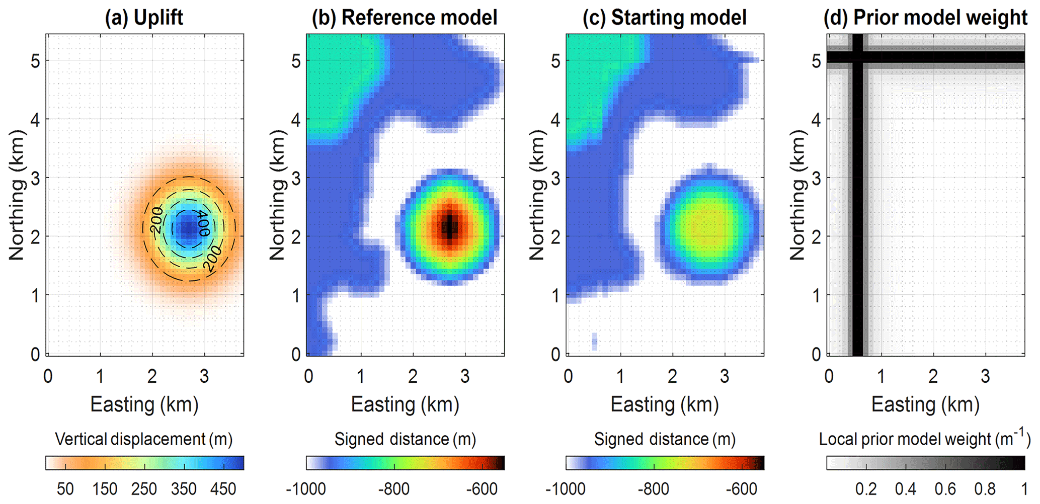
Figure 3(a) Dome added to the original model. (b) Reference model, with a signed-distance field of unit 1 at a depth equal to −1000 m. (c) Starting model, with signed-distance field of unit 1 at depth equal to −1000 m, (d) Weights Wp assigned to the prior model term in Eq. (4). We note that the starting model, as shown in panel (c), also corresponds to the prior model.
For our testing, we modified the original geological model further with the manual exaggeration of a dome present in the original model, which affects all units in the synthetic example (Fig. 3a). The resulting model is shown in Fig. 4a, where it is marked by the red arrow at the intersection of the two vertical slices. It is characterised by a vertical Gaussian displacement field with an amplitude of 500 m and a standard deviation of 350 m in both horizontal directions and centred around coordinates easting (2700 m) and northing (2125 m). We note from Fig. 3b that the added dome constitutes a noticeable difference with the starting model.
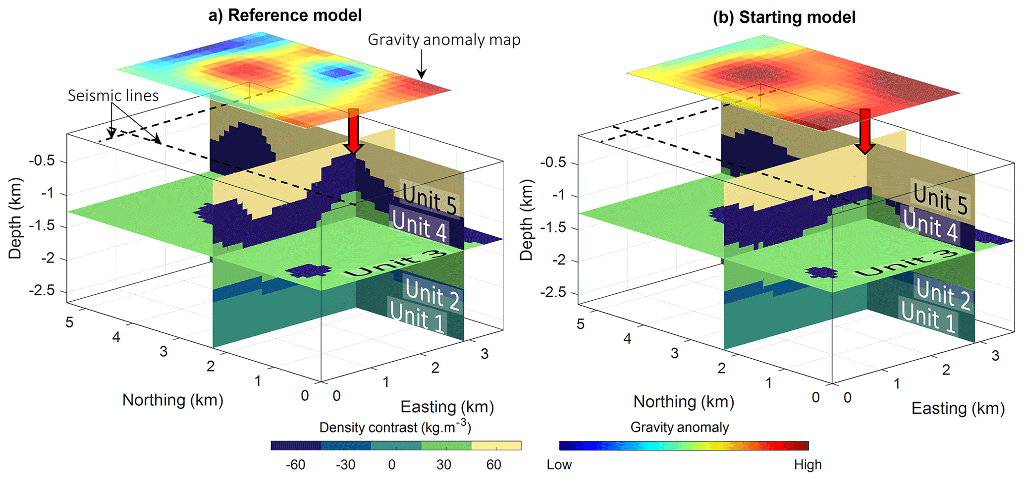
Figure 4Synthetic model for proof-of-concept testing. Reference model (a), with the corresponding gravity anomaly shown above the model. Starting model (b). The location of the seismic sections used to derive the prior model is shown by the dashed lines. The red arrows show the dome location. The two colour bars and their respective palettes are common to panels (a) and (b). This figure has been modified and adjusted from Giraud et al. (2022).
In what follows, we test the capability of the level-set-based inversion to recover the uplift, both without and with geological correction. We use a starting model in which the dome is nearly missing (see Fig. 3b for the example of unit 1 and Fig. 4b for a 3D view of the model), thereby simulating the scenario in which little to no indication about it is present in the 2D seismic and geological information. In addition to the dome, we increased the discrepancy between the starting model and the reference model by subsampling the reference geological dataset generating the starting model. It is obtained by retaining one out of every nine points of the original dataset (i.e. points from 2D surfaces) used to generate the reference model in LoopStructural. This generates fine-scale variations in the model, as can be seen from the comparison of Fig. 3b and c. From the comparison of the reference and starting gravity data (Fig. 4a and b, respectively), it appears that the perturbations of the reference model generate a strong starting data misfit for the starting model. We set up inversions such that ϕstart=ϕprior. To define the geological data dgeol used in the calculation of the geological correction term, as in Eqs. (7) and (8), we assume to only have knowledge of the stratigraphic column and of the average orientation of layers. In this example, the stratigraphic column is conformable, meaning that all geological layers are represented with one continuous relative geological time function. Consequently, the influence of geological correction is to guide or steer inversion towards a model with conformable layers arranged following the deposition order encoded in the stratigraphic column.
5.1.2 Inversion results and interpretation
Due to the overall simplicity of the model, the inversion converges in about 10 iterations and takes only a few seconds on a laptop computer. Inversion results are shown in Fig. 5.
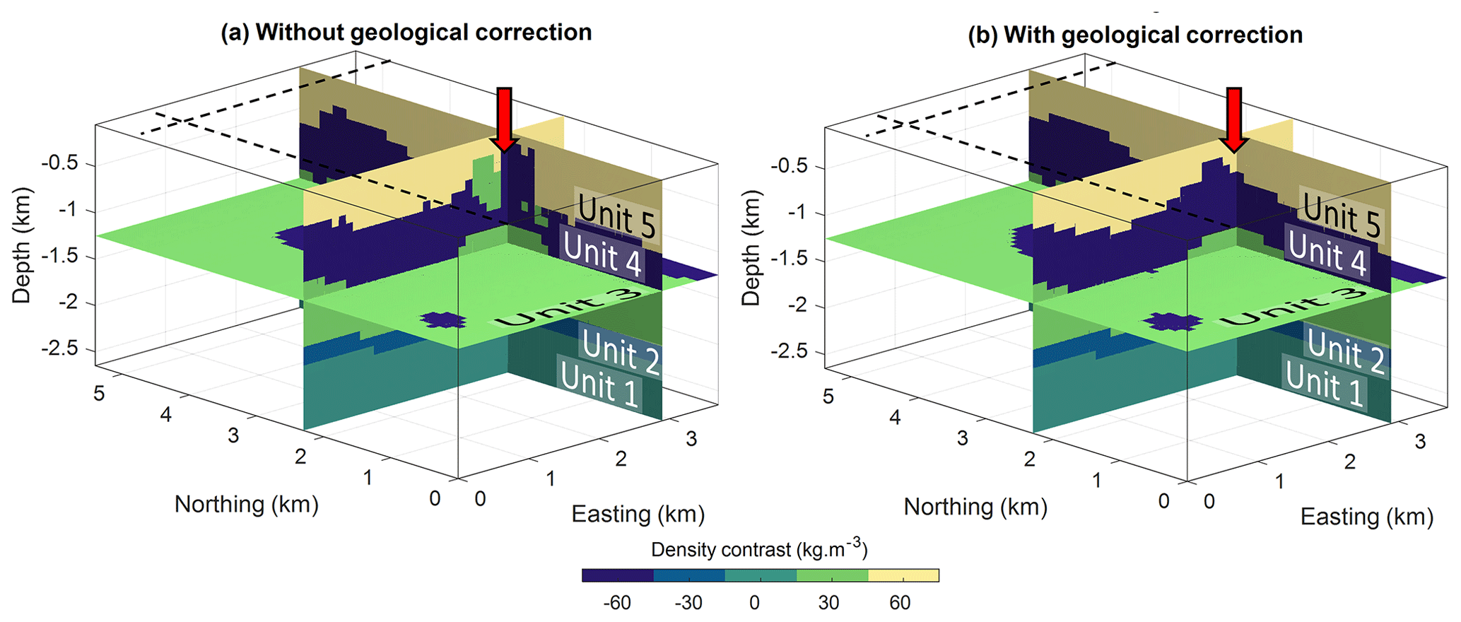
Figure 5Inversion results for the proof of concept: (a) without the application of geological correction (b) and using geological correction. This figure has been modified and adjusted from Giraud et al. (2022).
When no geological correction is applied (α=0 in Eq. 12), the requirement to only reduce the data misfit component of Eq. (4) (the evolution of which is shown in Fig. 4a and b) leads the inversion to produce geologically unfeasible features (abnormal stratigraphic contacts; Fig. 5a). On the contrary, consistent stratigraphic contacts and conformable stratigraphic units are obtained when the geological correction is applied with α=0.5 (Fig. 5b). Visually, the recovered model looks comparable to the reference model. Because the two recovered models have a different rock type representation, we consider other indicators to obtain a finer analysis. The value of α=0.5 was chosen without a rigorous analysis of its impact on the results. A naïve trial-and-error approach revealed that a value of 0.5 effectively “corrected” the course taken by uncorrected geophysical inversion and prevented the appearance of artefacts.
We complement our comparison of inverted models using the adjacency relationships introduced in Sect. 4.4. In a layered stratigraphy such the one as presented here, this can be useful for identifying geological contacts violating age relationships. In addition, it may be an indicator of the ruggedness of the surface contact as it measures the overall contact area. To compare the recovered models with the reference model, we calculate the difference between their respective adjacency matrices (Fig. 6). In Fig. 6a and b, we observe the occurrence of contacts absent from the reference model, where the adjacency between the units only follows the depositional order (the stratigraphic column; see Fig. 6d). Following geological rules, the contacts between units 3 and 5 recorded by the adjacency matrices of the starting model (Fig. 6a) and inversion without geological correction (Fig. 6b) should be forbidden. The comparison of adjacency matrices indicates that, in this case, inversion allows contact between units that are in disagreement with the reference model and which violate geological principles. It is interesting to note, however, that geophysical inversion reduces the number of such contacts, even in the absence of geological correction.
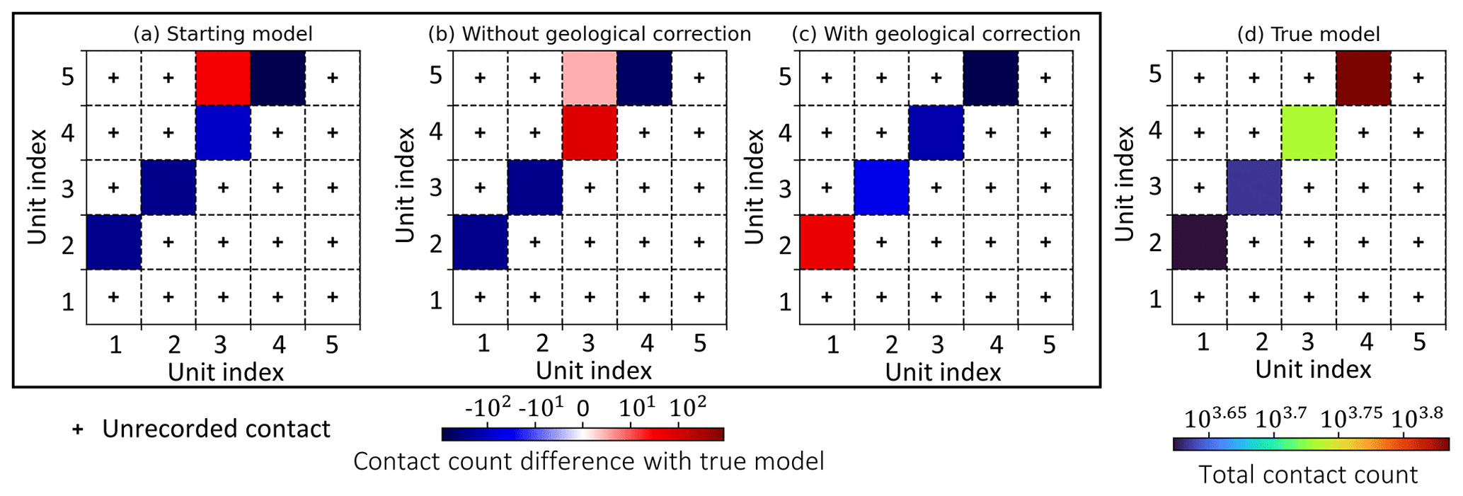
Figure 6Adjacency matrices showing differences between the true model and the starting model (a), inversion without geological correction (b), and inversion with geological correction (c). Panel (d) shows the adjacency matrix of the true model. Adjacency relationships are represented using upper triangular adjacency matrices, as the adjacency relationships are symmetric. The diagonal is left empty because we do not record the occurrences of a rock in contact with itself.
Furthermore, the geological correction term reduces the model search space to outcomes that are in agreement with the geological knowledge infused during inversion. While it is possible that such contacts come about at intermediate steps of the inversion, the convergence of the algorithm makes it unlikely for them to persist. As a consequence, no forbidden contacts are recorded in the adjacency matrix of inversion using geological correction (Fig. 6c).
From the success of this synthetic test, we have developed a structurally more complex model to investigate other features of the proposed algorithms and evaluate the limits of the integration method. While analysing the influence of inaccurate knowledge of densities in detail is beyond the scope of this paper, it remains important to ensure that inversions are robust to small errors in density. For this, we refer the reader to Appendix E, where we simulate errors in the knowledge of unit 4. Previous works using level inversion have investigated the importance of the starting model in the uncorrected case, and we assume that their conclusions hold. Likewise, we also assume the robustness of level-set inversions to noise, as shown by previous works cited in Sect. 1. To confirm this and for completeness, we performed additional tests, using
-
data contaminated with noise at a relatively high level compared to the amplitude of the uncontaminated data (Appendix C);
-
a degenerate starting model and data contaminated with noise (Appendix D); and
-
a starting model affected by errors in the density of rocks (Appendix E).
A detailed analysis of these tests is beyond the scope of this paper, and we refer the reader to these Appendices for more detail. In the remainder of this article, we assume that our approach is sufficiently robust in the presence of random noise and inaccurate starting models.
5.2 Testing the inversion approaches in the presence of an unconformity
In this section, we investigate a more challenging geological setting and explore the possibility of using automatic geological modelling to define the prior model term of the inversion's objective function. We also test the possibility of combining it with the application of geological correction to the model update. Additionally, we examine the possibility of using geological correction a posteriori to ensure geological realism (to “geologify”) in an existing model presenting features that conflict with the geological principles and/or data.
5.2.1 Survey set-up
We generate a synthetic model to test the proposed approach to recover information about objects other than conformable horizons such as unconformities. To this end, we generate a reference model resulting from three main geological events occurring in the following order (Fig. 8):
-
deposition of isopach stratigraphy made of four units and regional tilting;
-
sinistral faulting of these layers; and
-
erosion followed by a new depositional episode, leading to the observation of an angular unconformity.
These geological features can be produced using implicit modelling as described in the following. As explained above, in implicit geological modelling, all units within a conformable stratigraphic unit can be modelled using the same scalar field, which can be assimilated to a signed distance to some reference horizon. This signed distance represents conformable horizons where the value of the scalar field corresponds to the cumulative thickness from the base of the modelled series. The stratigraphic column defines the horizons based on these cumulative thicknesses. The rock units then correspond to thickness intervals which are associated with a rock model and are associated with density contrasts (see Figs. 7 and 8 for the resulting model). The orientation of parallel layers is governed by a vector indicating the direction towards younger strata (later referred to as the “younging” direction). The unconformity is assumed to be planar, so it is fully defined by a normal vector and a location point. This erosion surface separates two groups of stratigraphic units. For simplicity, we only consider a single rock unit overlaid with the unconformity (displayed in red in Fig. 7). The data used to generate the model are given in Appendix F, which provides quantities used in Eqs. (7)–(9). A view of the density contrast corresponding to this reference model is shown in Fig. 8.
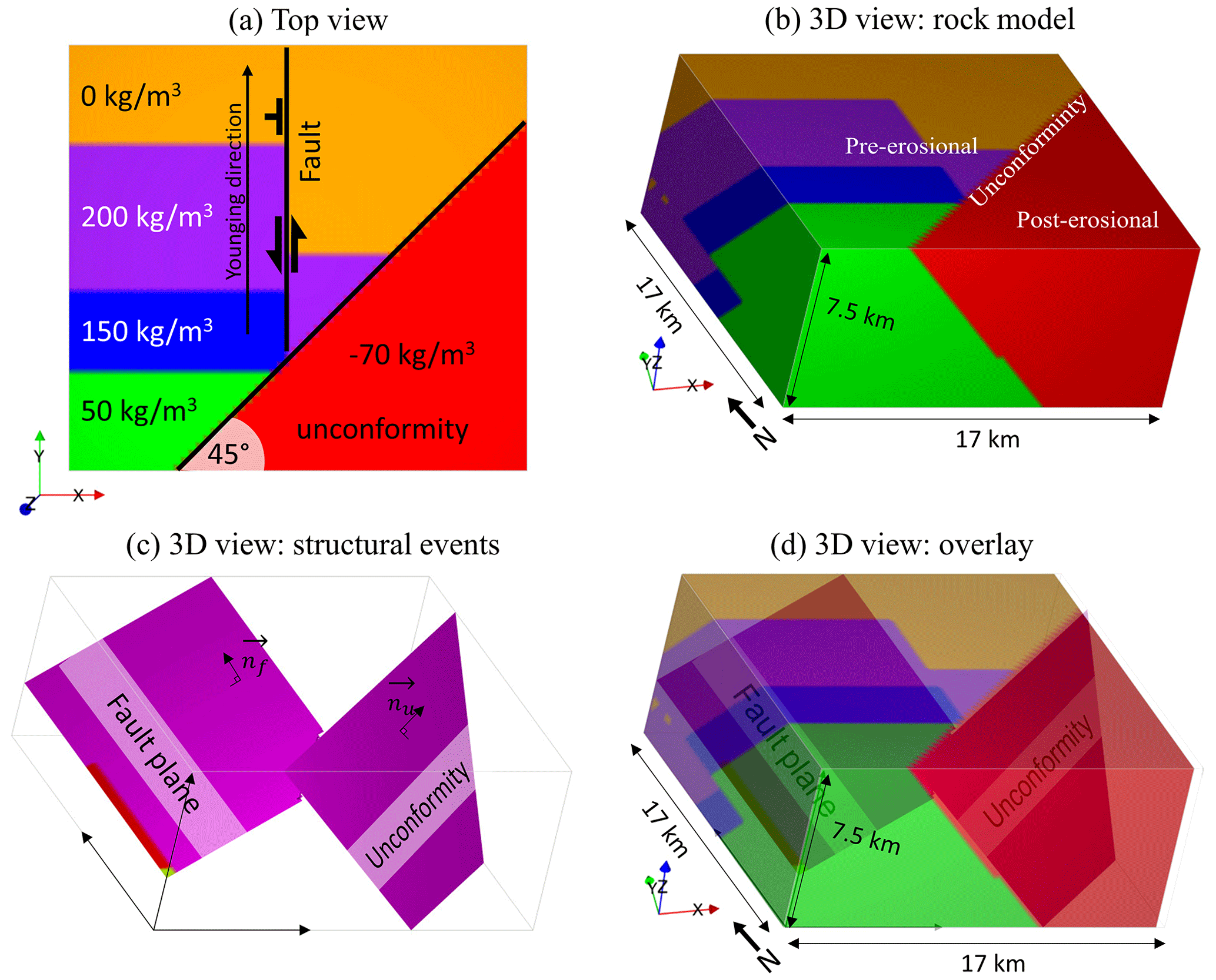
Figure 7Reference geological model and density contrasts. (a) Top view. (b) 3D rock unit cube. (c) Structural events overlaid with the rock model.
For our tests using this model, we consider a case in which the geological map defines the strike of the unconformity (Fig. 7a) and the fault orientation has been measured (the normal to the fault nf is available). However, in this fictitious scenario, the dip of the unconformity plane (hence, its normal nu) is not known and needs to be recovered. We assume that the erosion is planar, so there is only a lack of knowledge regarding the dip of the unconformity (equivalently, the vertical component of nu). The objective of this simple synthetic test is thus to estimate how accurately the unconformity can be modelled and, consequently, to determine whether we can retrieve the vertical component of nu and the model that gave rise to the observed measurements.
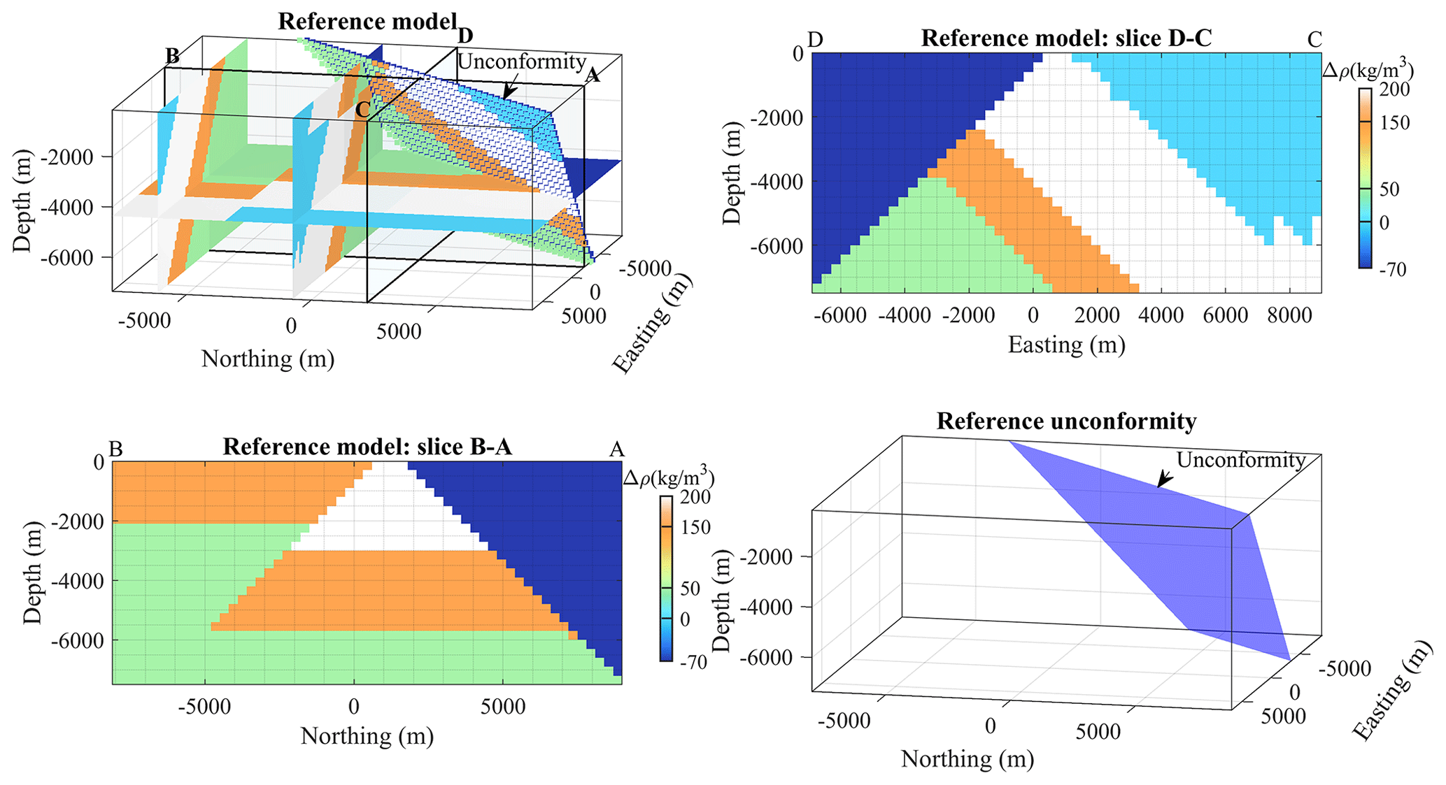
Figure 8Reference model visualised in a 3D view, in slices, and as a representation of the unconformity plane.
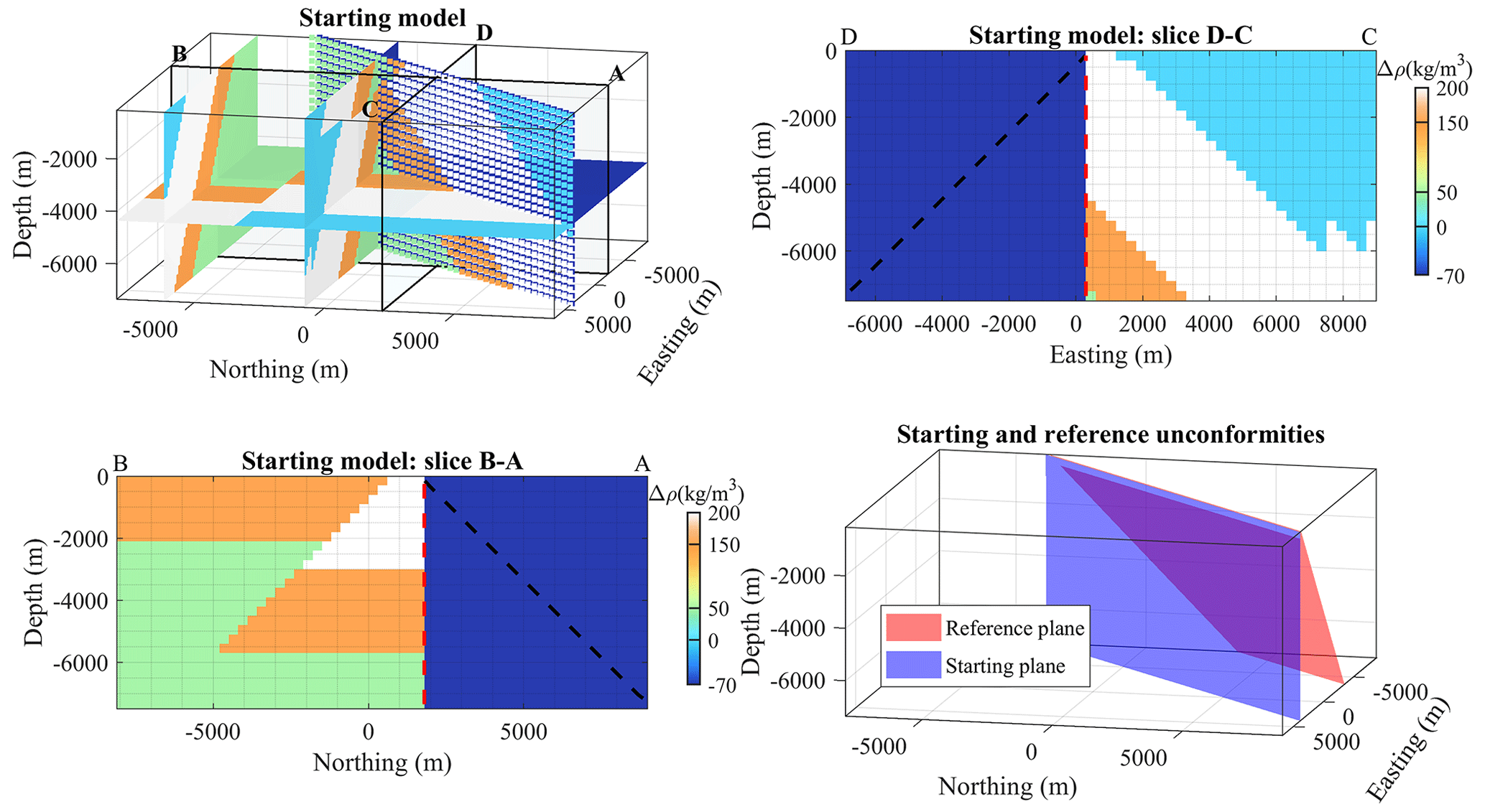
Figure 9Starting model visualised in a 3D view, in slices, and as a representation of the unconformity plane. The dashed black line represents the location of reference (or true) unconformity plane.
To test the geological components of inversion introduced in this paper, the following four geophysical inversion cases are investigated:
-
no use of implicit geological modelling during inversion;
-
geological modelling used to calculate a geological correction term to be applied to model updates (Sect. 3.3.1);
-
geological modelling used only to define the prior model term in the cost function of geophysical inversion (Sect. 3.3.2); and
-
geological modelling used in both the definition of the prior model term in the cost function and to calculate a geological correction term to be applied to model updates.
For the recovery of the unconformity plane (erosional surface), we separate the rock units into pre-erosional and post-erosional stratigraphic groups. The location of the contacts between these two groups is used for the calculation of a plane defining the unconformity, as detailed in Sect. 3.2.2. Assuming a complete lack of knowledge about the vertical component of nu, we set it to 0 (i.e. vertical unconformable contact) in the starting model for the inversion (Fig. 9). We run inversions corresponding to the four inversion scenarios proposed above. Inversions stop when they reach ERRd=0.5 mGal, which corresponds to an acceptable value for legacy data (Barnes et al., 2011). The gravity data simulated for the reference and starting models are shown in Fig. 10. We consider the data produced by the reference model to be the field measurements corresponding to the model that we try to recover. We assume zero error to test the ability of the method to recover the reference in perfect data settings (see Appendix C, D, and E for cases including data errors).
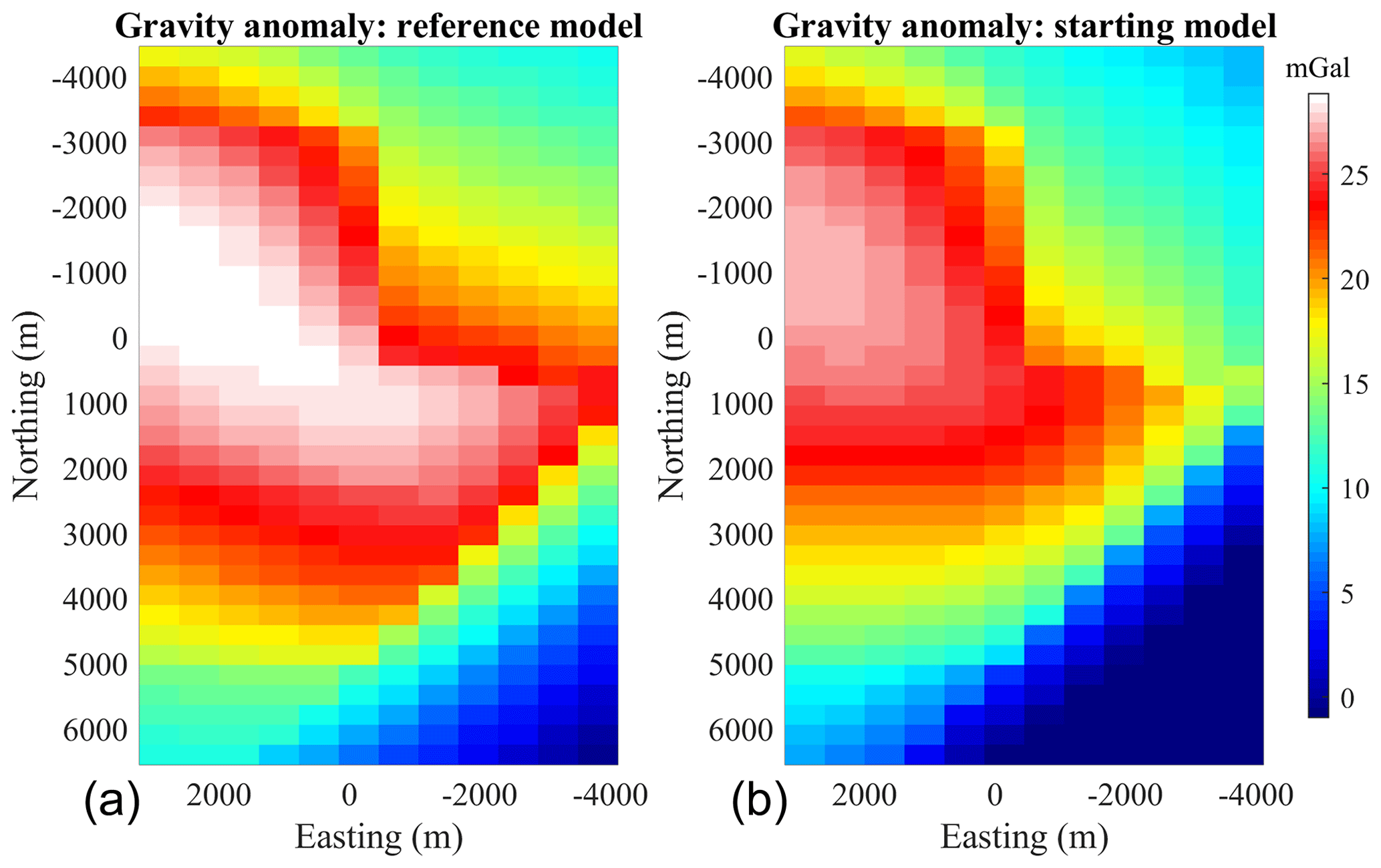
Figure 10Gravity data simulated for the reference model (a), which we consider to be the field data to honour, and for the starting model (b), which corresponds to the starting point of all inversion cases.
5.2.2 Inversion results
As a pre-requisite to comparing models, we point out that they are all geophysically equivalent from the point of view of the data misfit ERRd (Fig. 13a). On this basis, the features presented by the recovered models can be assessed from a geological and petrophysical perspective. Starting with a visual, qualitative interpretation of the results of the four scenarios listed above, we examine the following:
-
the 3D model, with the unconformity shown as scattered points in Fig. 11; and
-
the slices B–A and D–C in Fig. 12.
The main observation that can be made is that the unconformity boundary is poorly recovered for case (1) in the absence of either geological correction or a geological prior model term applied to the inversion. This is clearly visible in all images showing inversion results, be it from the 3D plot of points constituting the non-conformable contact (Fig. 11) or slices through the model (Fig. 12). This observation is further confirmed by the metrics shown in Fig. 13. Case (1), which considers geophysical data only in the inversion process, stands out for all metrics. For instance, ERRm remains notably higher when no geological modelling is used in the inversion than for all other cases (Fig. 13c). A similar behaviour is observed for OC and ERRΦ (Fig. 13b and d, respectively).
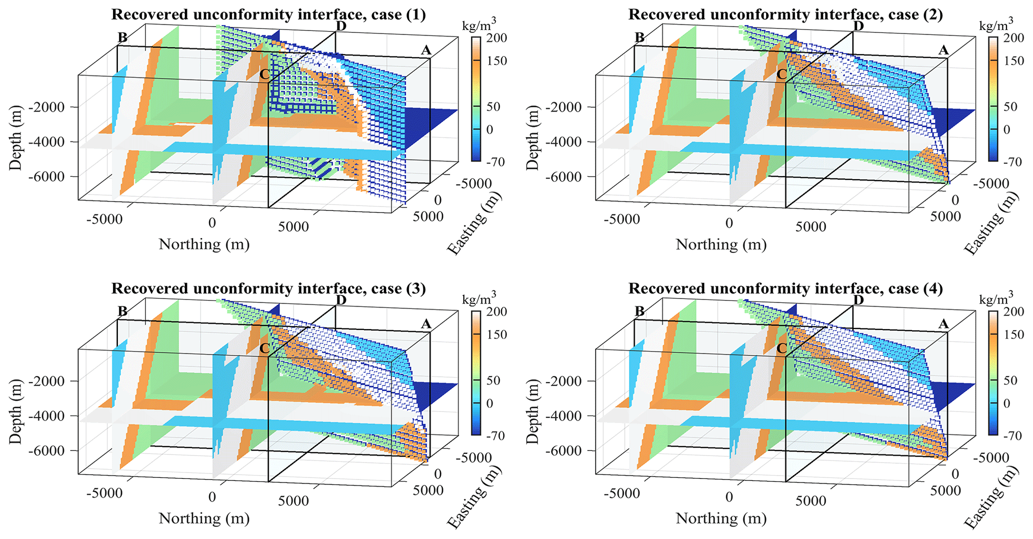
Figure 11Three-dimensional visualisation of the inversion results for cases (1) through (4). The differences between the best-fitting planes corresponding to the recovered uniformity interface shown here and the reference plane (Fig. 9) amount to 11.9, 3.2, 5.7, and 4.6∘ for cases (1) through (4), respectively.
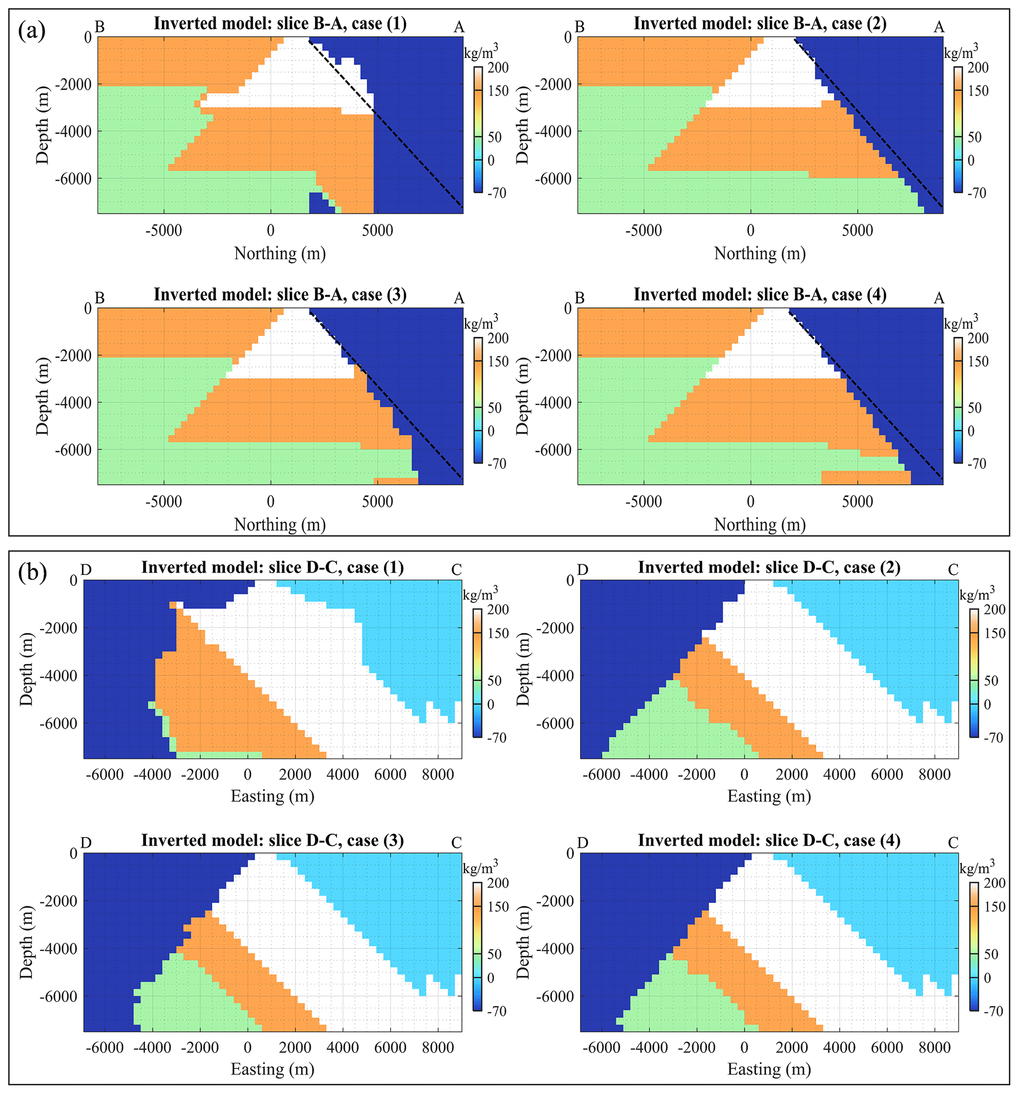
Figure 12Inversion results for cases (1) through (4) along sections B–A (a) and D–C (b). In panel (a), the true location of the unconformity is indicated by the dashed black line.
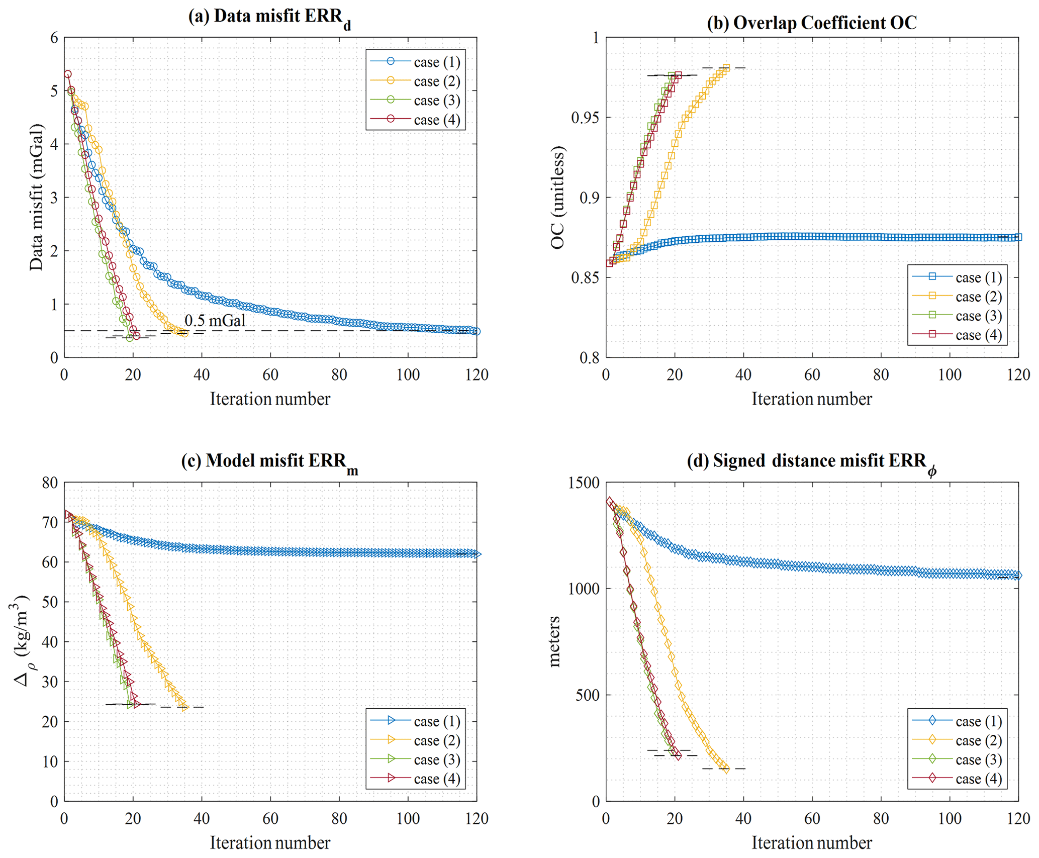
Figure 13Inversion metrics for cases (1) through (4), showing the data misfit (a), overlap coefficient (b), model misfit (c), and signed-distance misfit (d).
From this preliminary examination of the results for a relatively simple geological case, we conclude that using automatic geological modelling in inversion can dramatically increase the capability of the inversion, not only for recovering models consistent with geological data and principles but also for avoiding convergence to a local minimum when the starting model is inappropriate. This is true for both the application of a geological correction term or for the definition of a dynamic prior model term. Further to this, the convergence curves in Fig. 13a suggest that inversion considering geophysics alone may require many more iterations to converge when compared to using geological correction.
When visually comparing models from cases (2) and (3), it is clear that case (2) presents a contact between the non-conformable unit and the sequence that is slightly better recovered at depth than for cases (3) and (4) (Fig. 12). Cases (2), (3), and (4) are difficult to distinguish visually, except in the deeper part of the model, but this may be inconclusive due to the limited geological and geophysical sensitivity in this part of the model. Overall, a visual inspection suggests that case (2) seemingly has a higher degree of resemblance with the reference model while converging to a similar geophysical misfit. This is also suggested by the calculation of the dip angle of the recovered unconformity plane by automatic interpretation of the best-fitting plane. The difference with the reference model amounts to approximately 11.9, 3.2, 5.7, and 4.6∘ for cases (1) through (4), respectively.
Taken together, our results using this example suggest that
-
the use of geological modelling to define either a dynamic prior model or a correction term greatly increases the geological realism of the final model;
-
inversion using geological prior model term converges faster than otherwise; and
-
the use of a geological correction term may provide slightly better recovered unconformity planes.
5.3 Improving the geological realism of a pre-existing model
In this section, we investigate the possibility of increasing the geological realism of a pre-existing model provided a priori from, e.g., an already performed inversion or classification of the inversion results. To simulate this, we first start from the model inverted with the level set method without geological correction, as obtained in Sect. 5.1 (Fig. 14b), and run an inversion with the geological correction applied. The inverted model obtained in this fashion is shown in Fig. 14a. An animation showing the evolution of the inverted model together with geological inconsistences is shown in the Supplement provided by Giraud and Caumon (2023). The application of geological correction manages to remove a number of unrealistic features present in the starting model. However, the effect of the geological correction seems visually smaller than in the application of geological correction from the onset of inversion (Fig. 14c). Based on this premise, if large unrealistic features appear, then we recommend using the geological correction from the beginning of inversion instead of as an ad hoc process. We note that in the transition between Fig. 14a and b by the application of geological correction, all models are geophysically equivalent or nearly equivalent in that they present similar geophysical data misfit values. This suggests that, for this dataset, a continuum of models exists that fit the geophysical data to a similar level, while presenting different degrees of geological realism. In what follows, we investigate this possibility further, using the synthetic dataset presented in Sect. 5.2.
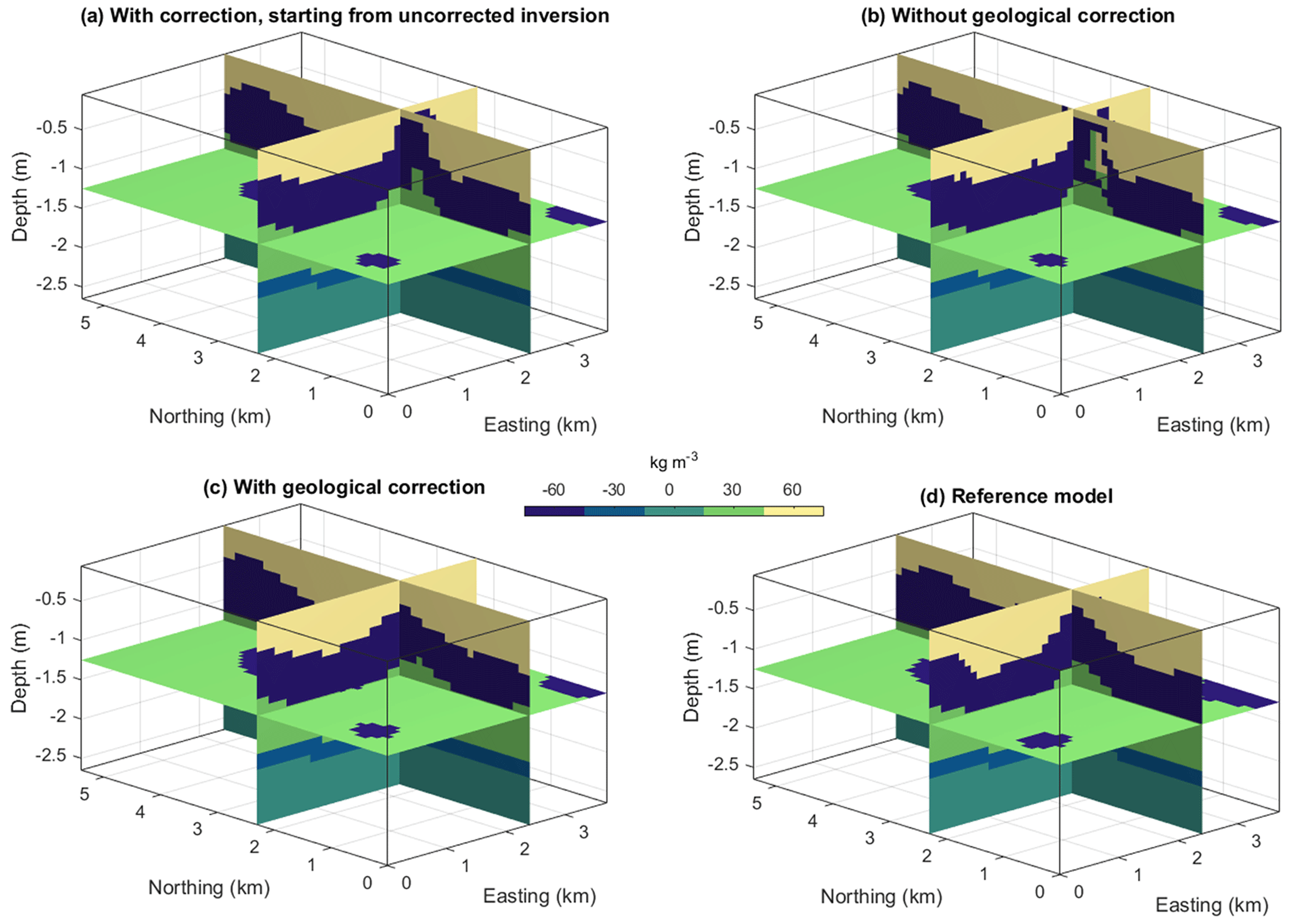
Figure 14Comparison of inversion results with (a) geological correction starting from inverted model obtained without geological correction, as shown in panel (b). Results with a geological correction (c). Reference model (d).
The starting model we consider for an improvement of the geological realism (Fig. 15a) shows very convoluted geometry for the unconformity and significant thickness variations in the pre-erosional sequence, while presenting a geophysical data misfit value ERRd close to the objective data misfit value of 0.5 mGal (dashed line in Fig. 13a). In real-world studies, this could correspond to the results of the rock type classification obtained a posteriori from geophysical inversion only or a legacy inversion. We will further refer to this case scenario as case (5). As can be seen in Fig. 15a, the starting model corresponding to case (5) is in strong disagreement with the reference model (Fig. 8) from a structural geological point of view as shown, for instance, by the high starting OC value (Fig. 16b). In particular, the unconformity is poorly recovered, and the expected planar contact is significantly distorted. In contrast, the layered stratigraphy is well resolved.
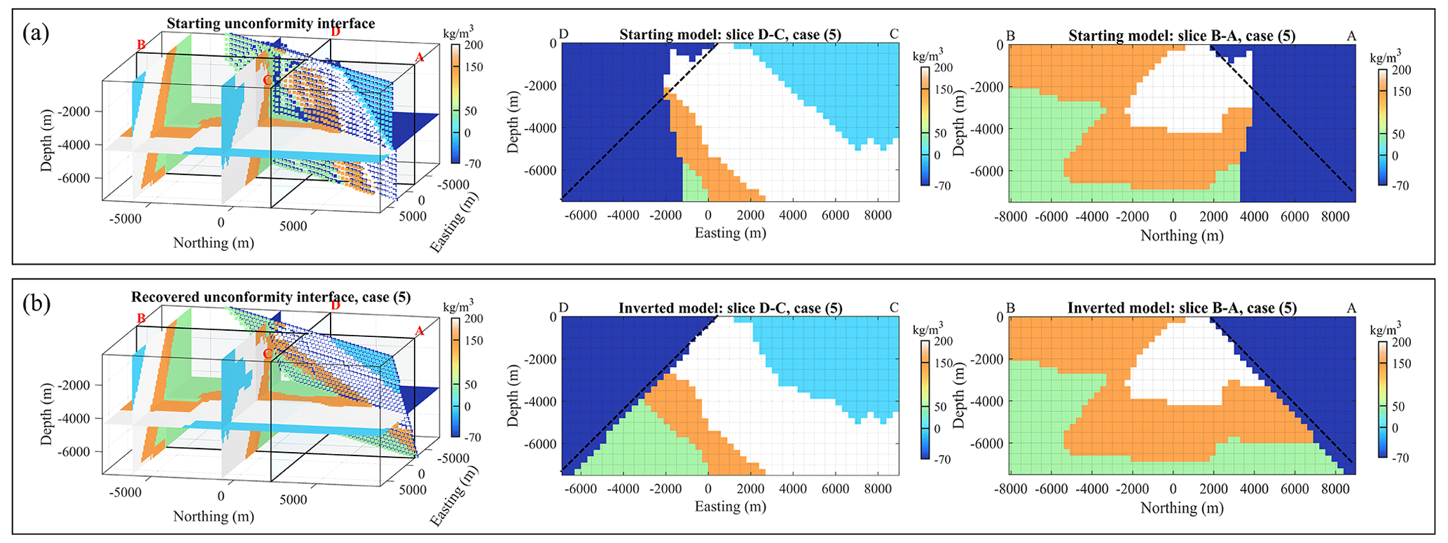
Figure 15(a) Starting model. (b) Inverted model. From left to right, the views are the same as those displayed in Figs. 11 and 12, respectively.
We use this model as a starting model for the inversion that applies only geological correction (Sect. 3.3.1; Eq. 4; flow (1) in Fig. 2). We use this case to evaluate the capability of our method to restore geological consistency between inversion results and geological observation while maintaining a geophysical data fit within the prescribed levels. As in the previous synthetic example, we focus the analysis on the unconformity, since it is the main feature targeted by the inversion in this example.
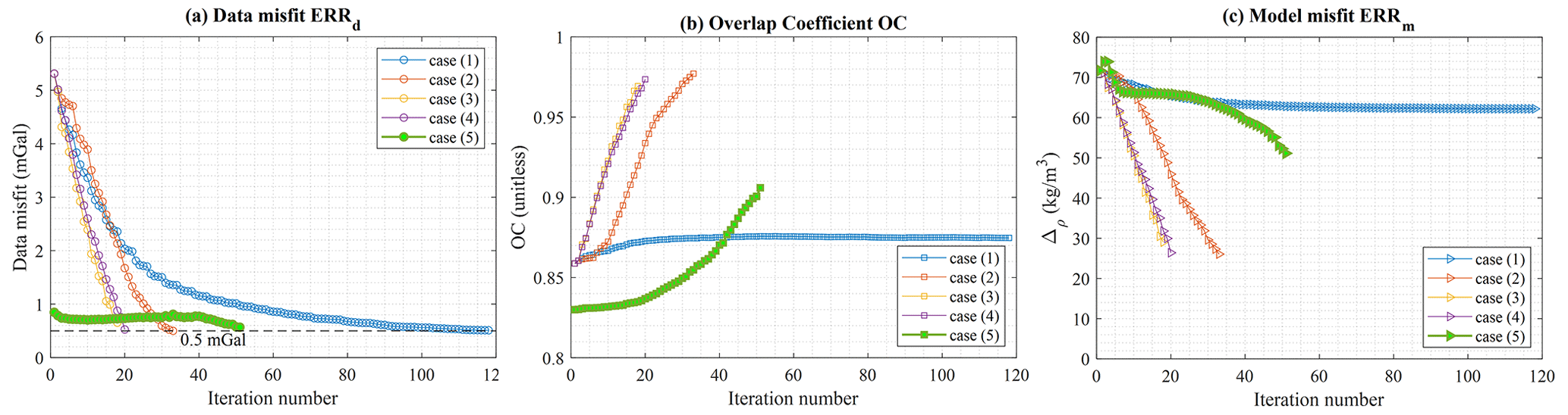
A visual inspection of inverted models shown in Fig. 16b indicates that the application of geological correction effectively drives the optimisation process towards models that are in better agreement with the unconformity observed in the geological map. However, the thickness variations in the pre-erosional sequence are only partly resolved. Nonetheless, the resulting model is in a region of the model space that is considerably closer to geologically plausible scenarios than the starting model. This is illustrated by the metrics used to monitor the inversion, which show an overall increase in the OC and a decrease in the model misfit ERRm (Fig. 16b and c, respectively). This implies that using a geological correction term may reduce the risk of the geophysical inversion converging to a geologically unrealistic local minima of the cost function.
In terms of geophysical data misfit, the data error ERRd presents a plateau that decreases only after iteration 40 (Fig. 16a), indicating the gradual deformation of models with similar ERRd values. This shows that the inversion navigates a region of the model space comprising models that are equivalent in terms of geophysical data misfit but which are gradually more consistent with the available geological data. This implies that the proposed approach may be effectively used to navigate the space of geophysically equivalent models. We note that the exploration of geophysically equivalent models can be performed using null-space shuttles to modify an already existing model, while maintaining a nearly constant geophysical data misfit (Deal and Nolet, 1996; Muñoz and Rath, 2006; Fichtner and Zunino, 2019). In our case, it could be achieved by the gradual deformation of the starting model to accommodate geological information. Based on these premises, the use of geological correction, as performed in this section, may open up avenues to
-
derive models not proposed by implicit geological modelling or geophysical inversion alone but through combining them instead; and
-
infuse geological data and principles into pre-existing inverted models derived without the knowledge or capability to integrate them.
6.1 Proposed work in the context of geoscientific exploration
In the last decade, the sampling of models from regions of the geological solution space to fit geological field observations has gained traction. The models proposed by these methods are usually derived from the interpolation of geological observations (Wellmann and Caumon, 2018). The inversion algorithm we proposed here can be used in conjunction with this strategy to modify such models using geophysical inversion. As geophysical inversion may be sensitive to features that geological modelling has little to no sensitivity to, geophysical inversion can be used to explore different regions of the solution space. This can be achieved with limited development efforts by using models that are representative of families sampled from the geological model space using, for example, topological analysis (Pakyuz-Charrier et al., 2019) or a similarity distance (Suzuki et al., 2008), to select starting models for inversion. Following the same idea, it may be possible to use deep learning for 3D geological structure inversion results (Jessell et al., 2022; Guo et al., 2021) as starting points to run series of inversions using the method presented here.
In some cases, geological modelling and geophysical inversion are difficult to reconcile. This may indicate that the modelling of geology is not sufficiently well informed by the available geological measurements and/or that hypotheses about the area need to be revisited. Under these circumstances, the geological model space might not contain a sufficiently good representation of the subsurface to fit the geophysical data. It could be the case, for instance, when structures are invisible to the available geological observations but can be sensed by geophysical data. In such cases, geophysical inversion, as performed here could be used as a tool to adjust these models and to infer the presence of unseen geological features.
As mentioned above, our inversion algorithm enables the estimation of the magnitude of adjustments required to reconcile geological models with geophysical measurements not only by comparing the forward response of the given models but also, and more importantly, by adjusting the model's geometry to fit the geophysical data. For scenario testing, the parameter controlling the amplitude of perturbation of interfaces between two successive iterations, τ, can be set accordingly with uncertainty information. For instance, it can be set arbitrarily small in locations of low uncertainty such as in the vicinity of boreholes, outcrops, or high-resolution seismic images. Following the same idea, τ could also be set using the uncertainty about domain boundaries derived using the implicit approach of Fouedjio et al. (2021). Further considerations of uncertainty may be required to better evaluate and understand the inversion results. For instance, the approach of Wei and Sun (2022), who generate a series of inverted models by varying their deterministic inversions' hyperparameters, could be a source of inspiration for uncertainty estimation. Likewise, the scalar field perturbation of Henrion et al. (2010), Clausolles et al. (2023), or Yang et al. (2019) could be transposed to the modelling approach we propose here.
We note that while experienced interpreters may be able to interpret geologically unrealistic inversion results “correctly”, it is nonetheless safer to ensure that geological principles are not violated by inversion. It removes an important source of uncertainty, and it reduces the impact of human bias and ambiguous interpretation, while ensuring that results can be robustly passed on to the next stage of modelling. More fundamentally, adding constraints essentially reduces the non-uniqueness of the inverse problem by making the search space smaller. In practice, however, more studies should be performed to assess whether the geological constraints change the “landscape” (or rugosity) or the objective function and to assess whether it always helps optimisation methods to avoid convergence to local minima.
Finally, the approach presented here belongs to a family of inversion approaches that could be referred to as “geometry driven”. That is, the main driver for fitting the geophysical data is the geometry of the subsurface model. One of our working assumptions is that the geological data used to derive structural geological models are complemented by geophysical data, with the possibility of altering the shape of geological models. Another geometry-driven approach consists of sampling points controlling the interpolated geological models within uncertainty and integrating their forward geophysical response to the calculation of a posterior distribution (Güdük et al., 2021; Liang et al., 2023). This method is very elegant, as it uses a unique geological level set parameterisation, but it does not explicitly address the integration of spatial geological data as provided by, e.g., drill holes. In contrast, our method can honour (up to discretisation errors) spatial data. The mapping of the geophysical signed distances ϕ onto their geological counterparts through fgeol makes it challenging to derive sensitivities directly like in Liang et al. (2023), but it probably makes it possible to explore a larger model space by possibly departing from geologically acceptable solutions during the non-linear iterations. Although further tests and comparisons between the two approaches are probably needed, this feature could be useful for preventing the optimisation from converging to local minima and could possibly be used in the future for stochastic inversions.
6.2 Limitations of the method and potential weaknesses
A potential limitation of the proposed approach that is inherent to the use of geological constraints pertains to the projection of an implicit rock model realisation onto the discrete mesh used to model geophysical data. Quoting Scalzo et al. (2022), “Naively exporting voxelised geology … can easily produce a poor approximation to the true geophysical [response]”. While it can be alleviated with the appropriate material averaging approach, aliasing can affect the geophysical response of the geological model projected onto the aforementioned mesh. This consideration is absent from our investigations, but it may be important to address in real-world case studies, where stakes are higher than in the work presented here.
A clear limitation of this work, which is intrinsic to the level set inversion, is the discreteness of the physical properties that are inverted for, which probably makes this kind of inversion one of the most parsimonious approaches. It presupposes accurate knowledge of the density of rock units and/or that they can be described by constant densities, neglecting geological and petrophysical phenomena leading to, for instance, lateral facies variations, compaction, and alteration. It is therefore possible for several rock types from the same stratigraphy to fall under the same “unit” in the modelling approach that we follow. Polynomials describing properties could be used instead of constant values. This limitation precludes the application of the method in certain scenarios. This may also call for integration with more advanced statistical rock physics and geostatistical modelling, using, for instance, the approach of Phelps (2016) to generate densities using a geostatistical approach. Additionally, porting the continuous value inversion component of the shape optimisation workflow of Dahlke et al. (2020) to 3D potential field inversion may help with generalising the potential use of level set inversion. Alternatively, the mapping from signed distances to a fixed-density value used here could be replaced by a mapping to an interval that defines the bound constraints enforced during inversion using the same approach as, e.g., Ogarko et al. (2021).
Finally, as mentioned in several places in the paper, further considerations on uncertainty are also required to better understand inversion results and find a set of admissible models, both geologically and geophysically.
6.3 Future research avenues
We formulate and solve the inverse problem in the least squares sense, using Tikhonov regularisation to stabilise the inversion and to infuse geological information. The regularisation functional we employ addresses only the difference between the proposed model and a given model. It is straightforward to consider other regularisation terms such as a gradient or Laplacian minimisation to encode geological information. Another avenue could be to use the same parameterisation for the geophysical and geological modelling and to solve for all information simultaneously.
In addition, the flexibility offered by the least squares framework allows for the design of constraint terms specific to the use of signed distances to enforce physical principles. For instance, one can think of maintaining the sum of the updates of signed distances to zero in each model cell such that, for the ith model cell, . This would preserve the signed-distance properties of ϕ at each iteration, thereby eliminating the need to reinitialise the signed-distance fields at each iteration using the fast-marching method.
The available geological information for constraining a geophysical inversion can take many forms, ranging from sparse information about rock properties to dense borehole data and seismic interpretations (Grana et al., 2012). We have explored the possibility of constraining a geophysical inverse model using surface geological data and seismic sections. Borehole information can without a doubt be considered in the same manner, and there is no restriction on the use of other sources of information, such as the modelling of other geophysical techniques (e.g. depth-to-basement from electromagnetic methods and reflectors from passive seismics).
An obvious and straightforward extension of this work is to extend it to magnetic data, the inversion of which shares many features with gravity inversion.
Finally, extensions of our method may allow for null-space exploration and the mitigation of some of the limitations identified in the previous subsection. This paper investigates the importance of geological information in a level set inversion. Previous work focusing on level set inversion and following an approach similar to ours has investigated the importance of accurate knowledge on the geometry and the number of rock units a priori (Giraud et al., 2021a). Giraud et al. (2021a) and Rashidifard et al. (2021) suggest that inversion is somewhat robust to errors in the starting model geometry and in the petrophysics of the rock units. Nonetheless, relatively small deviations between cases (2) and (5) illustrate that the proposed methodology is not sufficient to address the ill-posedness of the potential field inverse problem. Moreover, the results from Giraud et al. (2021a) suggest that level set inversion “presents limitations when an important geologic unit is missing from the initial model”. To alleviate this, ways to generate the “birth” of new geological units in order for inversion to consider geological bodies previously not accounted for due to the lack of information may be devised. One possibility could be to use the sensitivity of geophysical data to changes in the physical property. This may be useful, for instance, for modelling intrusions invisible to surface geology. Further to this, when starting from a discrete model resulting from level set inversion, it is possible to explore regions of the model space with intra-rock unit variations (lateral facies variations, compaction, etc.) simply through using the null-space shuttles, as proposed by Deal and Nolet (1996) and Fichtner and Zunino (2019). We believe that these two possibilities are two sides of the same coin that constitute a promising area of research for future work on uncertainty quantification.
We have introduced two novel approaches towards the unification of geological modelling and geophysical inversion into a deterministic inversion algorithm. They consist of
-
the application of a geological correction term to the geophysical inversion's model update,
-
the integration of automated geological modelling in a dedicated term of the objective function governing geophysical inversion,
and allow us to obtain inverse models that are consistent with geological principles and data.
These developments were motivated by the need to remediate some of the limitations inherent to geological and geophysical modelling when taken separately. We have shown that our framework is general in nature and can be applied in different contexts. We have tested the proposed approaches and demonstrated their potential using two synthetic examples, each representing a specific exploration scenario that is able
-
to constrain the modelling of a conformable stratigraphy, which relates to the deposition order of sediments; and
-
to recover the parameters of a tilted unconformity, which relates to tectonic history.
In both cases, the geological information used to derive constraints is sparse, and separate geological or geophysical modelling do not suffice to recover the reference model. We have shown experimentally that, in contrast, the integration of the two sources of information as proposed here provides the capability to recover models much closer to the reference structures and reduces the effect of the ill-posedness of the inverse problem. Our investigations also suggest that the methodology we propose can be applied with different goals in mind, including
-
complementing geological sampling techniques by automatically tuning implicit geological models to fit geophysical data;
-
deriving models as starting points to navigate the joint geology–geophysics null-space;
-
“geologifying” pre-existing models and exploring the geophysical space of equivalent models; and
-
recovering geological parameters and models in sparse data scenarios.
We derive the system of equations solved in the level set inversion scheme used here. Writing dcalc=Smm(ϕ), the system of equations corresponding to Eq. (4) is given as
At each iteration, the system is linearised around the current model. Solving for updates of the signed distances δϕ, we obtain, for the kth iteration,
Using the chain rule as in Eq. (5), we can rewrite the first element of the left-hand side of Eq. (A2) as follows and obtain the sensitivity matrix of the gravity data to changes in ϕ:
Sϕ‚ which relates the perturbation of signed distances to geophysical data, can be calculated from Eq. (2) and (3) (see Giraud et al., 2021a, for details about this derivation). Using Eq. (A3), the system of equations in Eqs. (A1) and (A2) is rewritten as
Wp is given as
where is a diagonal matrix of dimensions nm×nm locally adjusting the amount of change allowed to reach the signed-distance updates of the different model cells.
It is calculated as
where Σp is a diagonal matrix containing the uncertainty information derived from prior information. It can be used to control where the model updates are prioritised over other locations. In the absence of such prior information, Σp may be set as the identity matrix. 𝟙τ(ϕk) is the indicator vector of τi applied to ϕk. For the ith model cell, it is calculated as
As a consequence, is equal to zero for all cells not part of the inversion's domain (i.e. cells where 𝟙τ(ϕk) is null) and to one for all cells considered at any given iteration.
In this Appendix, we detail the calculation of the vector determining the orientation of an erosion plane, as mentioned in Sect. 3.2.2. It is calculated from the location of the contacts between rock units making up the modelled unconformity.
Let us define a plane by its normal vector n=[nx, ny, nz], and a real number s such that , where x is a coordinate vector in a three-dimensional space. The best-fitting plane approximating the contact between two units or groups of units is obtained by solving a linear equality-constrained least squares problem formalised as follows:
where b is a column vector of ones, and W is a diagonal matrix. It contains weights controlling the relative importance given to the different values in A, which contains the spatial coordinates of the points constituting the interface to be approximated as a planar contact. The matrix C contains the location of the contacts measured, e.g. at surface level from geological observations or from borehole data, which are used to define the equality constraints. d is a vector of ones. In our implementation, we solve Eq. (B1) using the open-source linear algebra library LAPACK proposed by Anderson et al. (1999), to which we refer the reader for further details.
In practice, W can be set according to the sensitivity of the geophysical data to variations in the physical property (sensitivity matrix S) in the model cells considered. To constrain the horizontal component of the normal vector calculated using the system of equations in Eq. (B1), two points located at surface level suffice. In this situation, we obtain an estimate of the third component of the normal vector to the plane, nz.
After obtaining the normal vector approximating the orientation of the plane, s can be determined from a location that the plane is known to cross (i.e. at the modelled interface), using the definition of the plane as .
We investigate the robustness of inversion with geological correction to random Gaussian noise, using the synthetic dataset introduced in Sect. 5.1.
We add noise with zero mean and a standard deviation equal to 0.075 mGal. This corresponds to 8 % of the absolute difference between the lowest- and highest-gravity anomaly value in the simulated dataset. We note that this value is superior to the case for a “carefully acquired and corrected” land survey, where a value of 0.05 mGal is acceptable (Barnes et al., 2011). The dataset with noise contamination, the forward data corresponding to the inverted model, their difference (i.e. the misfit map), and the noise that was added to the data are shown Fig. C1.
While the patterns that are visible in the difference map seem to be largely random, there might be a non-random component to the difference map, possibly due to the incomplete deformation of geological interfaces. We do not reproduce the resulting model, as it is visually largely similar to the case without noise in Fig. 5b.
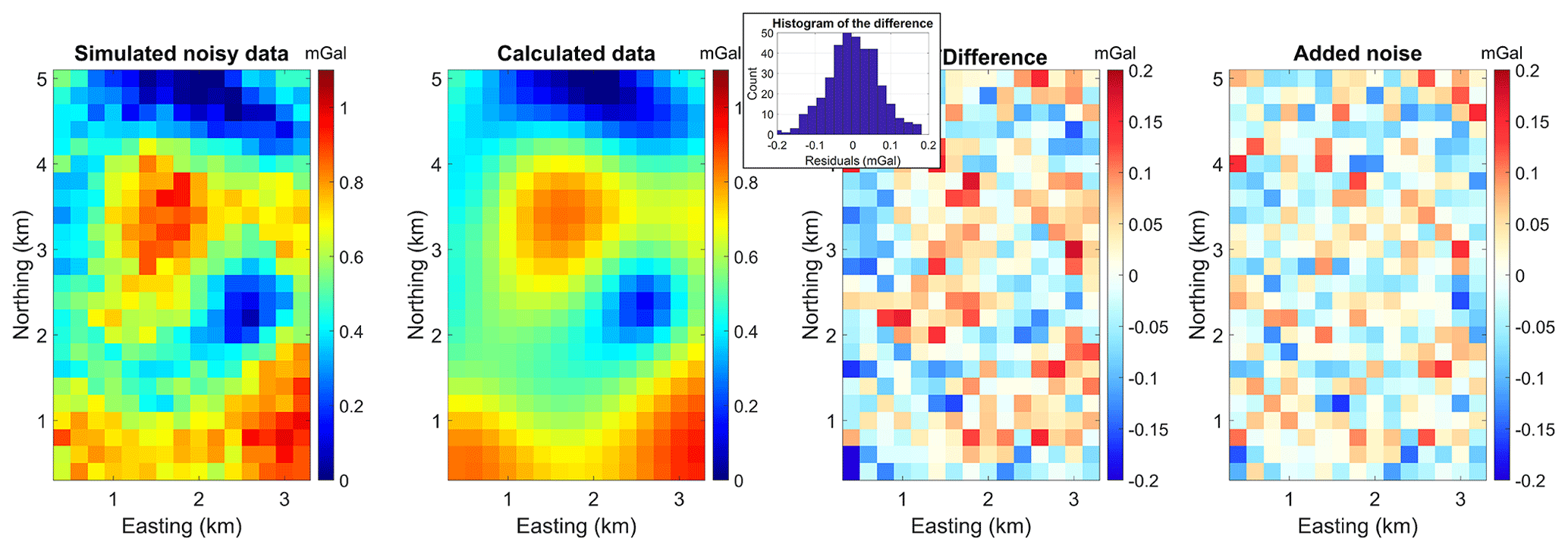
Figure C1Simulation of noisy data. From left to right, the data contaminated by noise, calculated data from the inverted model, the difference between inverted and calculated data with a histogram, and noise that was added to the data are shown.
In this Appendix, we are interested in testing the robustness of the method to changes in the starting model. For this, we use the same noisy dataset as in Appendix C and simulate a degenerate starting model. We rotate the starting model by 180∘ around the vertical axis. The so-obtained starting model and inverted model are shown in Fig. D1a and b, respectively. The starting data corresponding to this starting model are shown in Fig. D1c. When compared with the simulated field data (Fig. D1d), it is clear that this starting model is degenerate and presents an extreme scenario. Nevertheless, the inversion converges to a stable solution and manages to recover some of the features of the true model. However, the difference between the data that were inverted (Fig. D1d) and the calculated data (Fig. D1d) shows non-random patterns (Fig. D1f). This indicates that the inversion might be stuck in a local minimum and is thus unable to fit the data appropriately. This information notwithstanding, it is a confirmation that our approach is robust to errors in the starting model (to a certain degree) and to the presence of noise in the data. This also shows that in this example, the interaction between geological modelling and geophysical level set inversion leads to a reasonable solution with some realistic features, even though it is not sufficient to completely disambiguate the geophysical inverse problem.
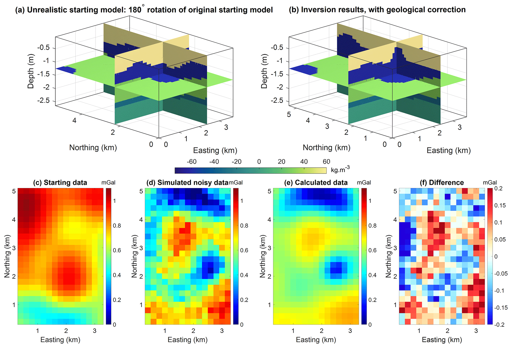
Figure D1Simulation of a degenerate case. The top row shows the starting (a) and inverted model (b). The bottom row shows the starting data (c), data contaminated by noise (d), calculated data from the inverted model (e), and the difference between inverted and calculated data (f).
In this Appendix, we investigate the impact of inaccurate estimations of the density of rock units, using the synthetic model presented in Sect. 5.1. We generate two starting models, considering the density contrast of unit 4 (dark blue unit in Fig. 4 and all figures showing this model).
-
In the first starting model, the absolute density contrast value is overestimated by 15 kg m−3.
-
In the second starting model, the absolute density contrast is underestimated by 15 kg m−3.
This leads to using density contrasts of −75 and −45 kg m−3, respectively, instead of −60 kg m−3. In this example, we use gravity data without noise contamination. The results are shown in Fig. E1, where we also remind the reader, for comparison, of the results obtained for the other tests we performed using this model. Figure E1b shows the inverted model using −75 kg m−3 for unit 4, which leads to a reduced overall volume of rock for unit 4. Figure E1b shows the inverted model with −45 kg m−3, which leads to an increased overall volume of rock for unit 4. In both cases, the overall geometry of the rock units is preserved when compared to the other cases and the reference model.
We note that this observation is in line with Giraud et al. (2021a), who do not consider the case with no geological correction. This experiment suggests that overestimating (underestimating) the difference in the density of a rock unit with its true values leads to underestimating (overestimating) its volume by increasing (decreasing) its overall volume while maintaining its overall shape.
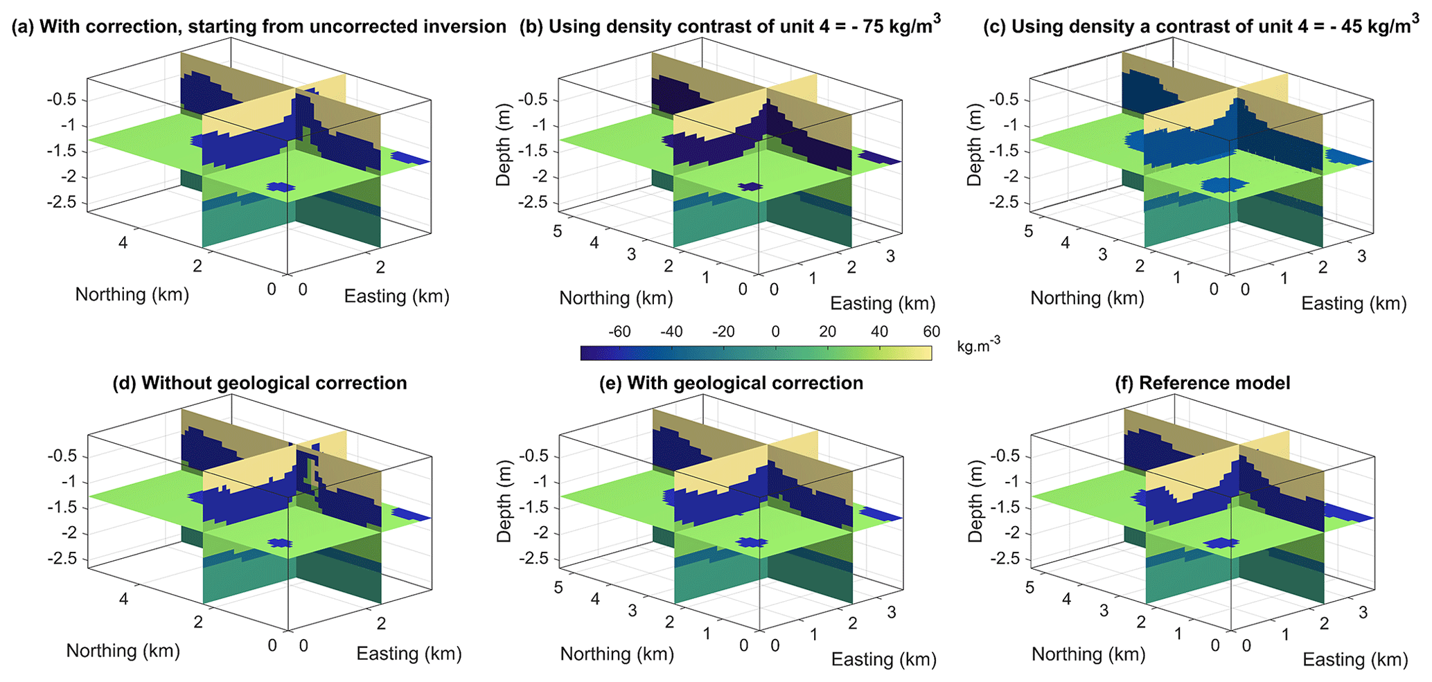
Figure E1Comparison of inversion results with (a) a geological correction, starting from the inverted model obtained without geological correction, as shown in panel (d). Results with a geological correction at each iteration with an underestimated density contrast (c) and overestimated density contrast (d) for unit 4. The case with accurate density contrast for all units and the reference model is shown in panels (d) and (e), respectively.
Table F1Geological data used to build the reference geological model.
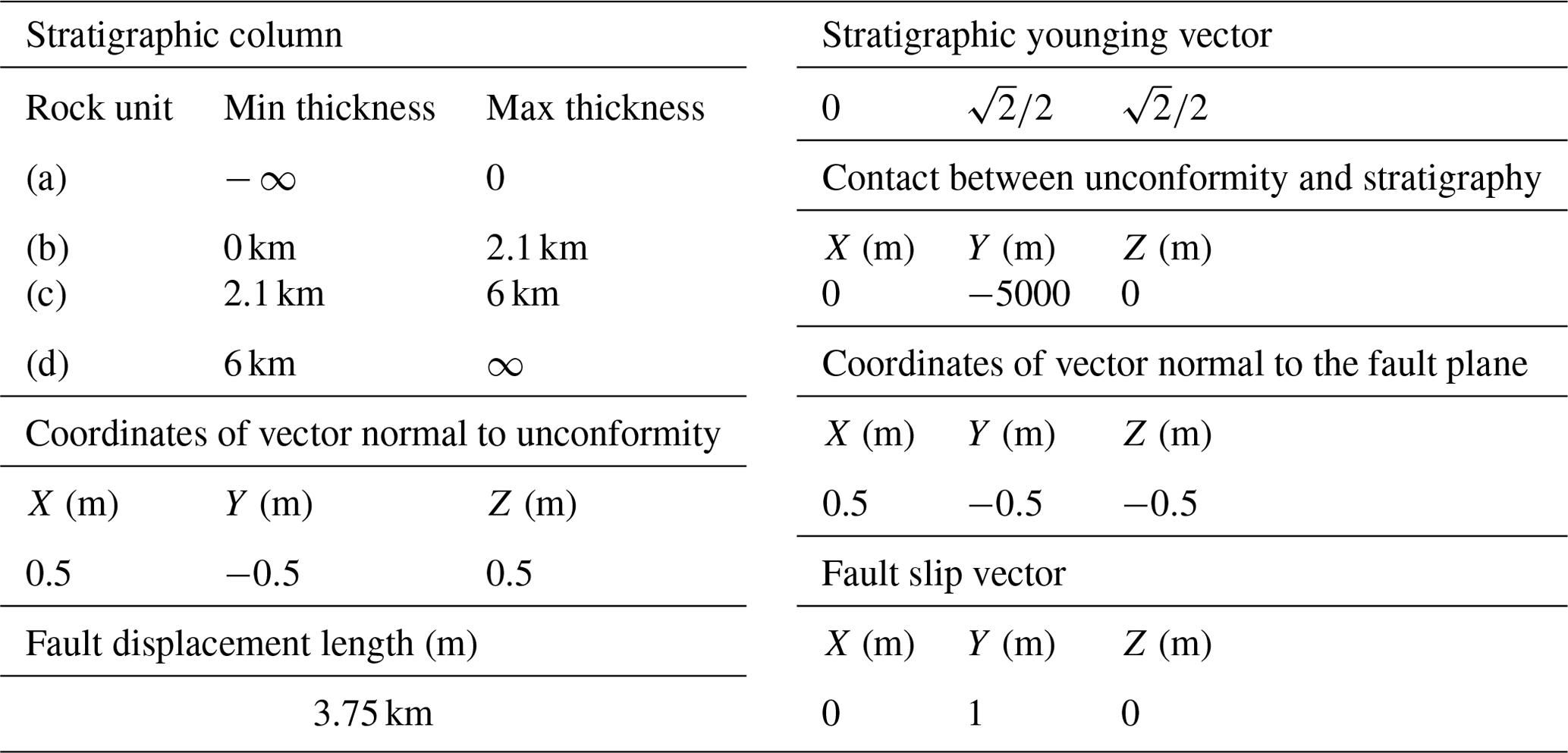
LoopStructural was made publicly available by Grose et al. (2020, https://doi.org/10.5281/zenodo.7542828). The latest version is available at https://github.com/Loop3D/LoopStructural. The geological data used to generate the models and the models shown here are provided in Giraud et al. (2023). The inversion used here is a prototype under development that will be released in the future as a GitHub repository associated with a paper. The Supplement is made available by Giraud (2023) (https://doi.org/10.5281/zenodo.7919381) and Giraud and Caumon (2023) (https://doi.org/10.5281/zenodo.7920886).
The supplement related to this article is available online at: https://doi.org/10.5194/se-15-63-2024-supplement.
JG conceptualised the project, with contributions from GC and LG; modified the original geological models generated by LG; conducted the geophysical modelling and inversion, with a peer review of the results with GC; developed and tested of the geophysical inversion code; developed and tested the link between geophysical inversion and geological modelling; analysed the results; wrote the paper, with comments from all other authors; and acquired the funding. LG created the geological model previously modified by JG, reviewed the paper, and contributed to the conceptual design of the method. PC took part in discussions with JG and GC, especially on model space exploration, and contributed to the editing of the paper. VO provided a critical review of the paper and gave extensive comments and suggestions.
The contact author has declared that none of the authors has any competing interests.
Publisher's note: Copernicus Publications remains neutral with regard to jurisdictional claims in published maps and institutional affiliations.
Jérémie Giraud acknowledges support from the European Union's Horizon 2020 research and innovation programme under the Marie Skłodowska-Curie Actions (grant no. 101032994). The authors also thank the RING (Research for Integrative Numerical Geology) and Loop Consortia (Loop : Enabling Stochastic 3D Geological Modelling) for their support. Vitaliy Ogarko acknowledges support from the Mineral Exploration Cooperative Research Centre, whose activities are funded by the Australian Government's Cooperative Research Centres Program. This is MinEx CRC document 2022/83.
This research has been supported by the European Union's Horizon 2020 research and innovation programme under the Marie Skłodowska-Curie Actions (grant no. 101032994) and by the Australian Research Council (grant no. LP210301239).
This paper was edited by Ulrike Werban and reviewed by three anonymous referees.
Anderson, E., Bai, Z., Bischof, C., Blackford, S., Demmel, J., Dongarra, J., Du Croz, J., Greenbaum, A., Hammarling, S., McKenney, A., and Sorensen, D.: {LAPACK} Users' Guide, 3rd Edn., Society for Industrial and Applied Mathematics, Philadelphia, PA., https://www.netlib.org/lapack/lug/ (last access: 24 September 2023), 1999.
Barnes, G. J., Lumley, J. M., Houghton, P. I., and Gleave, R. J.: Comparing gravity and gravity gradient surveys, Geophys. Prospect., 59, 176–187, https://doi.org/10.1111/j.1365-2478.2010.00900.x, 2011.
Calcagno, P., Chilès, J. P., Courrioux, G., and Guillen, A.: Geological modelling from field data and geological knowledge. Part I. Modelling method coupling 3D potential-field interpolation and geological rules, Phys. Earth Planet. Inter., 171, 147–157, https://doi.org/10.1016/j.pepi.2008.06.013, 2008.
Caumon, G., Lepage, F., Sword, C. H., and Mallet, J.-L.: Building and Editing a Sealed Geological Model, Math. Geol., 36, 405–424, https://doi.org/10.1023/B:MATG.0000029297.18098.8a, 2004.
Clausolles, N., Collon, P., Irakarama, M., and Caumon, G.: Stochastic velocity modeling for assessment of imaging uncertainty during seismic migration: application to salt bodies, Interpretation, 11, T361–T378, 1–67, https://doi.org/10.1190/int-2022-0071.1, 2023.
Collon, P., Pichat, A., Kergaravat, C., Botella, A., Caumon, G., Ringenbach, J.-C., and Callot, J.-P.: 3D modeling from outcrop data in a salt tectonic context: Example from the Inceyol minibasin, Sivas Basin, Turkey, Interpretation, 4, SM17–SM31, https://doi.org/10.1190/INT-2015-0178.1, 2016.
Cowan, J. and Beatson, R.: Rapid Geological Modelling, Australian Institute of Geoscientists Bulletin 36, Australian Institute of Geoscientists, Kalgoorlie, https://www.aig.org.au/publication-shop/digital-aig-bulletin-no-36-applied-structural-geology-for-mineral-exploration-and-mining/ (last access: 24 June 2023), 2002.
Dahlke, T., Biondi, B., and Clapp, R.: Applied 3D salt body reconstruction using shape optimization with level sets, Geophysics, 85, R437–R446, https://doi.org/10.1190/geo2019-0352.1, 2020.
Deal, M. M. and Nolet, G.: Nullspace shuttles, Geophys. J. Int., 124, 372–380, https://doi.org/10.1111/j.1365-246X.1996.tb07027.x, 1996.
De La Varga, M., Schaaf, A., and Wellmann, F.: GemPy 1.0: Open-source stochastic geological modeling and inversion, Geosci. Model Dev., 12, 1–32, https://doi.org/10.5194/gmd-12-1-2019, 2019.
Egenhofer, M. J.: A formal definition of binary topological relationships, in: Foundations of Data Organization and Algorithms, edited by: Litwin, W. and Schek, H. J., Lecture Notes in Computer Science, Vol. 367, Springer, Berlin, Heidelberg, https://doi.org/10.1007/3-540-51295-0_148, 1989.
Farquharson, C. G. and Oldenburg, D. W.: A comparison of automatic techniques for estimating the regularization parameter in non-linear inverse problems, Geophys. J. Int., 156, 411–425, https://doi.org/10.1111/j.1365-246X.2004.02190.x, 2004.
Fichtner, A. and Zunino, A.: Hamiltonian Nullspace Shuttles, Geophys. Res. Lett., 46, 644–651, https://doi.org/10.1029/2018GL080931, 2019.
Fouedjio, F., Scheidt, C., Yang, L., Achtziger-Zupančič, P., and Caers, J.: A geostatistical implicit modeling framework for uncertainty quantification of 3D geo-domain boundaries: Application to lithological domains from a porphyry copper deposit, Comput. Geosci., 157, 104931, https://doi.org/10.1016/j.cageo.2021.104931, 2021.
Frank, T., Tertois, A.-L., and Mallet, J.-L.: 3D-reconstruction of complex geological interfaces from irregularly distributed and noisy point data, Comput. Geosci., 33, 932–943, https://doi.org/10.1016/j.cageo.2006.11.014, 2007.
Galley, C. G., Lelièvre, P. G., and Farquharson, C. G.: Geophysical inversion for 3D contact surface geometry, Geophysics, 85, K27–K45, https://doi.org/10.1190/geo2019-0614.1, 2020.
Galley, C., Lelièvre, P., Haroon, A., Graber, S., Jamieson, J., Szitkar, F., Yeo, I., Farquharson, C., Petersen, S., and Evans, R.: Magnetic and Gravity Surface Geometry Inverse Modeling of the TAG Active Mound, J. Geophys. Res.-Sol. Ea., 126, e2021JB022228, https://doi.org/10.1029/2021JB022228, 2021.
Giraud, J.: Synthetic tests: unconstrained multiple level set inversions with errors in the starting model and noise in the data, Zenodo [data set], https://doi.org/10.5281/zenodo.7919381, 2023.
Giraud, J. and Caumon, G.: Evolution of model and geological inconsistencies during inversion, Zenodo [data set], https://doi.org/10.5281/zenodo.7920886, 2023.
Giraud, J., Ogarko, V., Lindsay, M., Pakyuz-Charrier, E., Jessell, M., and Martin, R.: Sensitivity of constrained joint inversions to geological and petrophysical input data uncertainties with posterior geological analysis, Geophys. J. Int., 218, 666–688, https://doi.org/10.1093/gji/ggz152, 2019.
Giraud, J., Lindsay, M., and Jessell, M.: Generalization of level-set inversion to an arbitrary number of geologic units in a regularized least-squares framework, Geophysics, 86, R623–R637, https://doi.org/10.1190/geo2020-0263.1, 2021a.
Giraud, J., Ogarko, V., Martin, R., Jessell, M., and Lindsay, M.: Structural, petrophysical, and geological constraints in potential field inversion using the Tomofast-x v1.0 open-source code, Geosci. Model Dev., 14, 6681–6709, https://doi.org/10.5194/gmd-14-6681-2021, 2021b.
Giraud, J., Caumon, G., Grose, L., and Cupillard, P.: Geometrical Inversion Coupled with Automated Geological Modelling, in: 83rd EAGE Annual Conference & Exhibition, European Association of Geoscientists & Engineers, 1–5, https://doi.org/10.3997/2214-4609.202210522, 2022.
Giraud, J., Caumon, G., and Grose, L.: Synthetic datasets used for numerical testing of geology-geophyiscs integration, Zenodo [data set], https://doi.org/10.5281/zenodo.7544954, 2023.
Gjoystdal, H., Reinhardsen, J. E., and Astebol, K.: Computer Representation Of Complex 3-D Geological Structures Using A New “Solid Modeling” Technique, Geophys. Prospect., 33, 1195–1211, https://doi.org/10.1111/j.1365-2478.1985.tb01359.x, 1985.
Godsil, C. and Royle, G.: Algebraic Graph Theory, 1–18, http://link.springer.com/10.1007/978-1-4613-0163-9_1 (last access: 24 September 2023), 2001.
Grana, D., Pirrone, M., and Mukerji, T.: Quantitative log interpretation and uncertainty propagation of petrophysical properties and facies classification from rock-physics modeling and formation evaluation analysis, Geophysics, 77, WA45–WA63, https://doi.org/10.1190/geo2011-0272.1, 2012.
Grose, L., Ailleres, L., Laurent, G., and Jessell, M. W.: LoopStructural (v1.5.5), Zenodo [code], https://doi.org/10.5281/zenodo.7542828, 2020.
Grose, L., Ailleres, L., Laurent, G., and Jessell, M.: LoopStructural 1.0: time-aware geological modelling, Geosci. Model Dev., 14, 3915–3937, https://doi.org/10.5194/gmd-14-3915-2021, 2021.
Güdük, N., de la Varga, M., Kaukolinna, J., and Wellmann, F.: Model-Based Probabilistic Inversion Using Magnetic Data: A Case Study on the Kevitsa Deposit, Geosciences, 11, 150, https://doi.org/10.3390/geosciences11040150, 2021.
Guillen, A., Calcagno, P., Courrioux, G., Joly, A., and Ledru, P.: Geological modelling from field data and geological knowledge. Part II. Modelling validation using gravity and magnetic data inversion, Phys. Earth Planet. Inter., 171, 158–169, https://doi.org/10.1016/j.pepi.2008.06.014, 2008.
Guo, J., Li, Y., Jessell, M. W., Giraud, J., Li, C., Wu, L., Li, F., and Liu, S.: 3D geological structure inversion from Noddy-generated magnetic data using deep learning methods, Comput. Geosci., 149, 104701, https://doi.org/10.1016/j.cageo.2021.104701, 2021.
Hansen, P. C. and Johnston, P. R.: The L-Curve and its Use in the Numerical Treatment of Inverse Problems, in: Computational Inverse Problems in Electrocardiography, 119–142, https://www.sintef.no/globalassets/project/evitameeting/2005/lcurve.pdf (last access: 24 September 2023), 2001.
Hansen, P. C. and O'Leary, D. P.: The Use of the L-Curve in the Regularization of Discrete Ill-Posed Problems, SIAM J. Sci. Comput., 14, 1487–1503, https://doi.org/10.1137/0914086, 1993.
Henrion, V., Caumon, G., and Cherpeau, N.: ODSIM: An Object-Distance Simulation Method for Conditioning Complex Natural Structures, Math. Geosci., 42, 911–924, https://doi.org/10.1007/s11004-010-9299-0, 2010.
Hoerl, A. E. and Kennard, R. W.: Ridge Regression: Application to nonorthogonal problems, Technometrics, 12, 69–82, https://doi.org/10.1080/00401706.1970.10488634, 1970.
Irakarama, M., Laurent, G., Renaudeau, J., and Caumon, G.: Finite Difference Implicit Structural Modeling of Geological Structures, Math. Geosci., 53, 785–808, https://doi.org/10.1007/s11004-020-09887-w, 2021.
Irakarama, M., Thierry-Coudon, M., Zakari, M., and Caumon, G.: Finite Element Implicit 3D Subsurface Structural Modeling, CAD Comput. Aided Des., 149, 103267, https://doi.org/10.1016/j.cad.2022.103267, 2022.
Jaccard, P.: Étude comparative de la distribution florale dans une portion des Alpes et du Jura, Bull. la Société Vaudoise des Sci. Nat., 37, 547–579, https://doi.org/10.5169/seals-266450, 1901.
Jayr, S., Gringarten, E., Tertois, A. L., Mallet, J. L., and Dulac, J. C.: The need for a correct geological modelling support: the advent of the UVT-transform, First Break, 26, 73–79, https://doi.org/10.3997/1365-2397.26.10.28558, 2008.
Jessell, M., Guo, J., Li, Y., Lindsay, M., Scalzo, R., Giraud, J., Pirot, G., Cripps, E., and Ogarko, V.: Into the Noddyverse: A massive data store of 3D geological models for machine learning and inversion applications, Earth Syst. Sci. Data, 14, 381–392, https://doi.org/10.5194/essd-14-381-2022, 2022.
Lelièvre, P. G. and Farquharson, C. G.: Integrated Imaging for Mineral Exploration, in: Integrated Imaging of the Earth: Theory and Applications, 137–166, https://agupubs.onlinelibrary.wiley.com/doi/10.1002/9781118929063.ch8 (last access: 24 September 2023), 2016.
Li, W., Lu, W., and Qian, J.: A level-set method for imaging salt structures using gravity data, Geophysics, 81, G27–G40, https://doi.org/10.1190/geo2015-0295.1, 2016.
Li, W., Lu, W., Qian, J., and Li, Y.: A multiple level-set method for 3D inversion of magnetic data, Geophysics, 82, J61–J81, https://doi.org/10.1190/geo2016-0530.1, 2017.
Li, W., Qian, J., and Li, Y.: Joint inversion of surface and borehole magnetic data: A level-set approach, Geophysics, 85, J15–J32, https://doi.org/10.1190/geo2019-0139.1, 2020.
Li, Y. and Oldenburg, D. W.: 3-D inversion of magnetic data, Geophysics, 61, 394–408, https://doi.org/10.1190/1.1443968, 1996.
Liang, Z., Wellmann, F., and Ghattas, O.: Uncertainty quantification of geologic model parameters in 3D gravity inversion by Hessian-informed Markov chain Monte Carlo, Geophysics, 88, G1–G18, https://doi.org/10.1190/geo2021-0728.1, 2023.
Moorkamp, M.: Integrating Electromagnetic Data with Other Geophysical Observations for Enhanced Imaging of the Earth: A Tutorial and Review, Surv. Geophys., 38, 935–962, https://doi.org/10.1007/s10712-017-9413-7, 2017.
Muñoz, G. and Rath, V.: Beyond smooth inversion: the use of nullspace projection for the exploration of non-uniqueness in MT, Geophys. J. Int., 164, 301–311, https://doi.org/10.1111/j.1365-246X.2005.02825.x, 2006.
Ogarko, V., Giraud, J., Martin, R., and Jessell, M.: Disjoint interval bound constraints using the alternating direction method of multipliers for geologically constrained inversion: Application to gravity data, Geophysics, 86, G1–G11, https://doi.org/10.1190/geo2019-0633.1, 2021.
Osher, S. and Fedkiw, R.: Level Set Methods and Dynamic Implicit Surfaces, edited by: Antman, S. S., Marsden, J. E., and Sirovitch, L., Springer, New York, NY, ISBN 0-387-95482-1, 2003.
Pakyuz-Charrier, E., Jessell, M., Giraud, J., Lindsay, M., and Ogarko, V.: Topological analysis in Monte Carlo simulation for uncertainty propagation, Solid Earth, 10, 1663–1684, https://doi.org/10.5194/se-10-1663-2019, 2019.
Pellerin, J., Caumon, G., Julio, C., Mejia-Herrera, P., and Botella, A.: Elements for measuring the complexity of 3D structural models: Connectivity and geometry, Comput. Geosci., 76, 130–140, https://doi.org/10.1016/j.cageo.2015.01.002, 2015.
Phelps, G.: Forward modeling of gravity data using geostatistically generated subsurface density variations, Geophysics, 81, G81–G94, https://doi.org/10.1190/geo2015-0663.1, 2016.
Rashidifard, M., Giraud, J., Lindsay, M., Jessell, M., and Ogarko, V.: Constraining 3D geometric gravity inversion with a 2D reflection seismic profile using a generalized level set approach: application to the eastern Yilgarn Craton, Solid Earth, 12, 2387–2406, https://doi.org/10.5194/se-12-2387-2021, 2021.
Renaudeau, J., Malvesin, E., Maerten, F., and Caumon, G.: Implicit Structural Modeling by Minimization of the Bending Energy with Moving Least Squares Functions, Math. Geosci., 51, 693–724, https://doi.org/10.1007/s11004-019-09789-6, 2019.
Scalzo, R., Lindsay, M., Jessell, M., Pirot, G., Giraud, J., Cripps, E., and Cripps, S.: Blockworlds 0.1.0: a demonstration of anti-aliased geophysics for probabilistic inversions of implicit and kinematic geological models, Geosci. Model Dev., 15, 3641–3662, https://doi.org/10.5194/gmd-15-3641-2022, 2022.
Sethian, J. A.: A fast marching level set method for monotonically advancing fronts, P. Natl. Acad. Sci. USA, 93, 1591–1595, https://doi.org/10.1073/pnas.93.4.1591, 1996.
Souche, L., Lepage, F., Laverne, T., and Buchholz, C.: Depositional Space: Construction and Applications to Facies and Petrophysical Property Simulations, in Day 2 Mon, December 07, 2015, IPTC, https://doi.org/10.2523/IPTC-18339-MS, 2015.
Sprague, K. B. and de Kemp, E. A.: Interpretive Tools for 3-D Structural Geological Modelling Part II: Surface Design from Sparse Spatial Data, Geoinformatica, 9, 5–32, https://doi.org/10.1007/s10707-004-5620-8, 2005.
Suzuki, S., Caumon, G., and Caers, J.: Dynamic data integration for structural modeling: model screening approach using a distance-based model parameterization, Comput. Geosci., 12, 105–119, https://doi.org/10.1007/s10596-007-9063-9, 2008.
Szymkiewicz, D.: Une conlribution statistique à la géographie floristique, Acta Soc. Bot. Pol., 11, 249–265, https://doi.org/10.5586/asbp.1934.012, 2017.
Tarantola, A.: Inverse Problem Theory and Methods for Model Parameter Estimation, Society for Industrial and Applied Mathematics, https://epubs.siam.org/doi/book/10.1137/1.9780898717921 (last access: 26 September 2023), 2005.
Thiele, S. T., Jessell, M. W., Lindsay, M., Ogarko, V., Wellmann, J. F., and Pakyuz-Charrier, E.: The topology of geology 1: Topological analysis, J. Struct. Geol., 91, 27–38, https://doi.org/10.1016/j.jsg.2016.08.009, 2016.
Wei, X. and Sun, J.: 3D probabilistic geology differentiation based on airborne geophysics, mixed Lpnorm joint inversion and physical property measurements, Geophysics, 87, K19–K33, https://doi.org/10.1190/geo2021-0833.1, 2022.
Wellmann, F. and Caumon, G.: 3-D Structural geological models: Concepts, methods, and uncertainties, in: Advances in Geophysics, edited by: Schmelzbach, C., Cambridge, Massachusetts, 1–121, ISBN 9780128152089, 2018.
Wellmann, J. F., de la Varga, M., Murdie, R. E., Gessner, K., and Jessell, M.: Uncertainty estimation for a geological model of the Sandstone greenstone belt, Western Australia – insights from integrated geological and geophysical inversion in a Bayesian inference framework, Geol. Soc. Lond. Spec. Publ., 453, SP453.12, https://doi.org/10.1144/SP453.12, 2017.
Yang, L., Hyde, D., Grujic, O., Scheidt, C., and Caers, J.: Assessing and visualizing uncertainty of 3D geological surfaces using level sets with stochastic motion, Comput. Geosci., 122, 54–67, https://doi.org/10.1016/j.cageo.2018.10.006, 2019.
Zheglova, P., Farquharson, C. G., and Hurich, C. A.: 2-D reconstruction of boundaries with level set inversion of traveltimes, Geophys. J. Int., 192, 688–698, https://doi.org/10.1093/gji/ggs035, 2013.
Zheglova, P., Lelièvre, P. G., and Farquharson, C. G.: Multiple level-set joint inversion of traveltime and gravity data with application to ore delineation: A synthetic study, Geophysics, 83, R13–R30, https://doi.org/10.1190/geo2016-0675.1, 2018.
- Abstract
- Introduction
- Geometrical inversion: formalisation
- Integrating structural geological modelling into geophysical inversion
- Metrics for the evaluation of inversion results
- Synthetic application cases
- Discussion
- Conclusions
- Appendix A: Building the least squares system of equations
- Appendix B: Estimating the best-fitting plane of a contact under constraints
- Appendix C: Robustness to noise
- Appendix D: Robustness to a degenerate starting model with noisy data
- Appendix E: Robustness to errors in the density of rock units
- Appendix F: Geological data
- Code and data availability
- Author contributions
- Competing interests
- Disclaimer
- Acknowledgements
- Financial support
- Review statement
- References
- Supplement