the Creative Commons Attribution 4.0 License.
the Creative Commons Attribution 4.0 License.
 | 19 Jul 2024
Quantifying mantle mixing through configurational entropy
Erik van der Wiel
Cedric Thieulot
Douwe J. J. van Hinsbergen
Geodynamic models of mantle convection provide a powerful tool to obtain insights into the structure and composition of the Earth's mantle that resulted from a long history of differentiating and mixing. Comparing such models with geophysical and geochemical observations is challenging, as these datasets often sample entirely different temporal and spatial scales. Here, we explore the use of configurational entropy, based on tracer and compositional distribution on a global and local scale. We show means to calculate configurational entropy in a 2D annulus and find that these calculations may be used to quantitatively compare long-term geodynamic models with each other. The entropy may be used to analyse, with a single measure, the mixed state of the mantle as a whole and may also be useful to compare numerical models with local anomalies in the mantle that may be inferred from seismological or geochemical observations.
- Article
(12236 KB) - Full-text XML
- BibTeX
- EndNote


Mantle convection models that are used to simulate the evolution and dynamics of the solid Earth are built on different sets of observations, each providing its own constraints to validate the state of the mantle through time (e.g. Dannberg and Gassmöller, 2018; Gerya, 2014). For instance, with the advent of full-plate kinematic reconstructions of the past hundreds of million years (e.g. Domeier and Torsvik, 2014; Merdith et al., 2021), mantle models can now be driven by plate motions through geological time (e.g. Coltice and Shephard, 2018; Flament et al., 2022; Heister et al., 2017). Such experiments then lead to a prediction of the structure and composition of the mantle that may be compared to geological, geochemical or seismological observations from the modern Earth (e.g. Bower et al., 2015; Flament et al., 2022; Li et al., 2023; Lin et al., 2022; Yan et al., 2020).
Key observables of the modern Earth that may be predicted by models are anomalies in mantle structure or composition that result from mantle mixing or the absence thereof. For instance, seismic tomography provides images of the present-day mantle as relatively slow and fast regions in terms of seismic wave propagation, which can relate to variations in temperature and/or composition such as slabs or mantle plumes (Koelemeijer et al., 2017; Ritsema and Lekiæ, 2020). The heterogeneity of the Earth's mantle is also reflected in geochemical observations of magmatic rocks, ocean island basalts (OIBs) and mid-oceanic ridge basalts (MORBs), which suggest the existence of depleted, enriched and even primordial mantle reservoirs, i.e. unmixed regions that maintain a geochemically distinct composition (Jackson et al., 2018; Jackson and Macdonald, 2022; McNamara, 2019; Stracke et al., 2019). Notably, seismological and geochemical heterogeneities may entirely, partly or hardly overlap, and observations may relate to spatial and temporal scales. Seismology reveals seismic velocity anomalies in the mantle on scales of hundreds to thousands of kilometres, varying from slabs to LLSVPs (e.g. (Garnero et al., 2016; Ritsema et al., 2011; van der Meer et al., 2018). Geochemical differences between MORBs from the Atlantic, Pacific and Indian oceans indicate compositional heterogeneity on a hemispheric scale (Doucet et al., 2020; Dupré and Allègre, 1983; Hart, 1984; Jackson and Macdonald, 2022), and geochemical zonation within a single plume system is evidence for heterogeneities on a 100 km scale (Gazel et al., 2018; Hoernle et al., 2000; Homrighausen et al., 2023; Weis et al., 2011), whereas micro-scale analysis even reveals major variations between samples (Stracke et al., 2019). All such variations may result from a cycle of geochemical differentiation and renewed mixing that is associated with mantle convection and that may eventually be predicted by mantle convection models. To this end it is important to also be able to define or quantify the mixed state of the modern mantle from a suitable numerical mantle convection model on the relevant range of spatial scales. While mixing technically involves diffusion at small scales and the term stirring has been proposed to account for the mechanical stretching and folding (Farnetani and Samuel, 2003), which is in fact our interest here, we shall nevertheless use the term mixing in the remainder of the article, as we use varying “compositions” that are able to mix.
It has long been recognized that mantle convection is complex, and its mixing has been studied for decades (see Kellogg, 1993, and van Keken et al., 2003, for early reviews on this topic). Unsurprisingly, the advent of high-performance numerical modelling in the mid-90s saw a resurgence in the characterization of mantle mixing and its quantification. Various approaches have been proposed over the years, but the vast majority of these are based on the time evolution of a swarm of particles. Early studies (such as Hoffman and McKenzie, 1985; Olson et al., 1984a, b; Richter et al., 1982; Schmalzl et al., 1996) use statistics to arrive at a mixing timescale. Another approach using the presence, addition and/or removal of particles in a modelled domain is used to quantify mixing times and degassing (sampling of primitive mantle) (Gottschaldt et al., 2006; Gurnis and Davies, 1986a, b) to measure strain and the dispersal of tracers (Christensen, 1989; Kellogg and Turcotte, 1990) or to study the development of time-dependent mantle heterogeneities (Hunt and Kellogg, 2001). Note that other methods have been proposed, such as a line method (Ten et al., 1998), a correlation dimension method (Stegman et al., 2002) and a hyperbolic persistence time method (Farnetani and Samuel, 2003).
More recently, another approach has dominated the mantle mixing literature: it consists of measuring the Lyapunov time, which is the characteristic timescale for which a dynamical system is chaotic, or rather its inverse, the Lyapunov exponent. By evaluating the Lyapunov exponent, it can be shown that mixing is laminar or turbulent; the larger the exponent, the more efficient the mixing is. A typical example uses a steady-state velocity pattern obtained in a 3D spherical domain to advect passive particles (van Keken and Zhong, 1999). It uses a very common approximation to the Lyapunov exponent, i.e., the finite-time Lyapunov exponent, which is based on the evaluation of the distance between a multitude of particle pairs that are initially very close to each other (i.e., stretching of this original distance after 4 Ga). This shows a strong diversity in mixing behaviour dependent on the mantle flow characteristics. Other studies that used the same approach in studying a variety of mantle convection problems include Bello et al. (2014), Bocher et al. (2016), Colli et al. (2015), Coltice (2005), Coltice and Schmalzl (2006), Farnetani et al. (2002), Farnetani and Samuel (2003), Ferrachat and Ricard (1998, 2001), Samuel et al. (2011), Tackley and Xie (2002), and Thomas et al., 2024.
In this study, we investigate the merits of yet another approach, the configurational (or “Shannon”) entropy for quantifying compositional mixing of particles through flow on a global or local scale (Shannon, 1948). Despite its popularity in other fields, it has only minimally been used in geosciences (e.g. Camesasca et al., 2006; Naliboff and Kellogg, 2007). We develop the application of configurational entropy to the 2D cylindrical mantle convection models which we recently developed (van der Wiel et al., 2024), implementing measures for local and global entropy of mixing that incorporate information on composition. We aim to use configurational entropy to quantify the degree of mixing on different scales for different hypothetical initial compositional configurations of the mantle and the evolution thereof over time. Subsequently, we discuss how configurational entropy may be used as a bridge for quantitative comparison between mantle convection models and geological, seismological or geochemical observations.
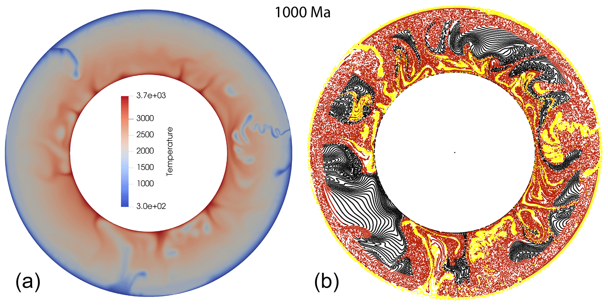
Figure 1Snapshot from model R at t = 1000 Ma showing the temperature field in Kelvin (a) and passive particles coloured by composition (lithosphere: yellow; upper mantle: red; lower mantle: black) (b).
2.1 Mixing entropy
Configurational entropy is analogous to the Shannon entropy (Shannon, 1948) and related to the probabilities derived from the distribution of particles with a certain value, i.e., composition. It can be used to track the mixing of particles independently of the physical process causing that mixing in numerical simulations and in laboratory experiments. This entropy is widely used and has a large variety of applications, including fluid- or magma mixing (Camesasca et al., 2006; Naliboff and Kellogg, 2007; Perugini et al., 2015), transport of plastic in oceans (Wichmann et al., 2019), distribution of seismicity in earthquake populations (Goltz and Böse, 2002) and the quantification of uncertainty in geological models (Wellmann and Regenauer-Lieb, 2012).
The definition of the configurational entropy S is based on the proportion of a specific distribution of particles in a domain tessellated by non-overlapping cells. For this we use passive particles, or tracers, that are advected in a flow model leading to particle trajectories. The entropy depends on the distribution of particles, the number of cells and the initial compositional distribution (see Sect. 2.3). Let C be the number of compositions and M the number of cells in the domain. The entropy is calculated based on the discretized particle density ρc,j (Eq. 1), i.e., the number of particles of composition c in cell j,
where Nc is the total number of c particles divided by the number of cells M. This assumes that cells are of equal area, and it will be used here in our 2D application. Hence, Nc is the same for all cells. From the compositional density ρc,j we calculate Pj,c, which is the proportion of particles of composition c in cell j relative to the total number of particles in the cell, both measured in terms of density through Eq. (2). We calculate Pj through the cell sum of all compositional densities in Eq. (3). Pj is the proportion of the amount of particles in a cell relative to all the particles in the system. The quantities we describe here as proportions would be regarded as probabilities, or conditional probabilities, in statistical physics.
Next, Eq. (4) defines the global entropy Spd of the particle distribution.
which quantifies the global spatial heterogeneity of the particle distribution independently of composition (Naliboff and Kellogg, 2007). At the cell level, the local entropy Sj for cell j can be defined for the mixture of particles with different compositions:
Finally, the global entropy S of the particle distribution, accounting for composition, is the weighted average of Pj (Eq. 3) and the local entropy Sj (Eq. 4) through Eq. (6) (Camesasca et al., 2006).
Maximum entropy is achieved when all particle densities ρc,j are equal; i.e., the distribution of composition and the number of particles are the same in each cell. Each entropy above has a different maximum which depends on either the number of cells (for Spd) or the number of compositions used (for S and Sj). To compare entropies between mixing models with different initial conditions, we normalize the entropies by dividing each by its maximum. The maximum for Spd is equal to ln M, while for Sj and S the maximum is ln C (Camesasca et al., 2006). This provides values for all entropies between the endmembers 0 (entirely segregated composition) and 1 (uniformly mixed). The maximum value for Spd can only be reached when all compositions are present in equal ratios. Entropy calculations of four simple educational examples are shown and explained in Appendix A to help the reader appraise these quantities.
2.2 Mantle convection model
We apply the configurational entropy to the quantification of mixing in a recently developed 2D numerical mantle model in a 2D cylindrical geometry that simulates 1000 Ma of ongoing mantle convection and subduction (van der Wiel et al., 2024). The convection model was designed to evaluate the sensitivity of inferred lower-mantle slab-sinking rates (van der Meer et al., 2018) to the vigour of mantle convection. The simulations comprised dynamically self-consistent, one-sided subduction below freely moving, initially imposed continents at the surface, culminating in slab detachment followed by the sinking of slab remnants across the lower mantle (Fig. 1). The surface velocity in the model was generally between 1 and 4 cm a−1, which may be compared to the reconstructed values of 4 cm a−1 of Zahirovic et al. (2015), and the obtained average slab-sinking rates were in the range of those that were inferred from correlations between the location of imaged lower-mantle slabs and their geological age (van der Meer et al., 2018). This modelling qualitatively illustrates the degree of mixing in a modelled mantle and the potential preservation of an unmixed original mantle, advected slabs, or (partly) homogenized mixed mantle shown by the distribution of particles.
We quantify the degree of mantle mixing in the model by investigating the local and global mixing entropies (Sect. 2.1) for model R of van der Wiel et al. (2024) at different resolutions. We also illustrate how mixing entropy quantifies the mixing of a different model (model P) that showed significantly higher slab-sinking rates than inferred for the lower mantle and that displayed a higher degree of mantle mixing (van der Wiel et al., 2024). For this purpose, we only used the passive particle distribution available from the models in van der Wiel et al., 2024. The cells used to calculate the configurational entropy (see Sect. 2.4) are independently substantiated and therefore not the same as those used in the numerical model. For any additional information on these models we refer the reader to van der Wiel et al., 2024.
2.3 Initial composition
To illustrate how we track compositional evolution with configurational entropy, we assign a compositional distribution to our example models with two different approaches. In case A, we assign a compositional distribution in the initial model, and each tracer will keep its initial composition through time. We divide the annulus into two concentric parts at a radius of 5100 km and assign the inner and outer part a different composition (simply put: a different colour). This creates a ratio between the number of particles of each composition. Case B uses dynamic compositions; i.e., the composition of a particle may change over time. We use three compositions whose relative ratios are allowed to change over time depending on the particle's depth in the model. Initially, we define particles as lower mantle when they start below 660 km depth in the model, upper mantle if they start between 100 and 660 km depth, and lithosphere if they start between 0 and 100 km depth. Particles keep their “lower-mantle” composition as long as they do not ascend above 660 km depth during model evolution. Any particle that moves from a deeper reservoir into a shallower one will see its composition changed to the shallower reservoir and will maintain this composition for the remainder of model time. This approach is an example that may be used in a study to characterize the secular geochemical differentiation of the solid Earth.
2.4 Cell distribution
Entropy as calculated in this study also depends on the number and distribution of cells, which is independent of the mesh used in the numerical model itself. To ensure an approximately equal cell area throughout our domain, we vary the number of cells per radial layer. The cell area is determined by the product of the radial extent δr and lateral extent δθ that follows from the number of radial layers and the number of cells along the core–mantle boundary (CMB) circumference. Varying cell area may be important to compare the outcome of a numerical model with datasets that have very different resolutions (e.g. seismology versus geochemistry). We illustrate different cell resolutions with our 2D example model, but a similar approach may be used for a 3D model, albeit with a different tessellation (Thieulot, 2018). One should note that in this setup our cells are chosen to be of equal area, while in a 3D model this should be equal volume.
The lowest resolution (10 × 40) contains 40 cells along the CMB, increasing across the 10 layers to 68 cells along the surface, for a global total of 539 cells (Fig. 2). The highest resolution that we illustrate (20 × 160) then gives a global total of 4430 cells (Fig. 2). The numerator ρc,j for the proportion calculations (Eqs. 2 and 3) for cells that do not contain a particle ( would cause a problem in its contribution to the entropy via the natural logarithm. Note that xln x=0 and that cells without a particle therefore do not add to any of the entropies; these cells are skipped in practice in the summation of Eqs. (4)–(6).
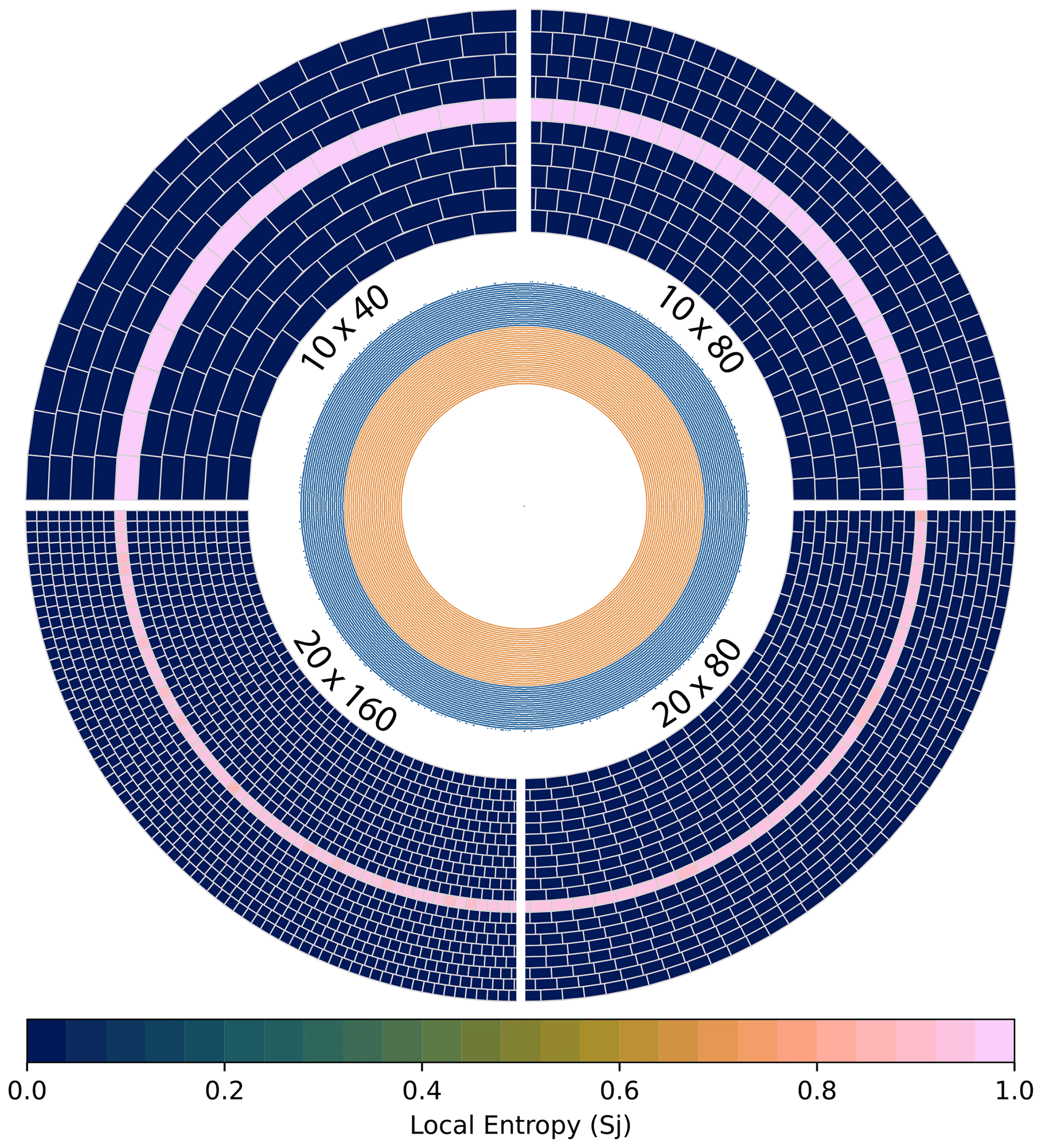
Figure 2Representation of the various tested resolutions. Shown is the initial (t = 0 Ma) particle distribution (inner annulus) and local entropy Sj (outer annulus) for the static composition distribution (case A). The cells with a high Sj (pink) indicate that both compositions are present, and the unmixed cells (blue) contain only one composition.
In this section, we describe the various obtained entropies, starting with the particle distribution Spd. Next, we underline the importance of resolution for the local entropy Sj in our example model at different resolutions for the static composition distribution (case A) and show how the local entropy evolves over time. Finally, we show the temporal evolution of the global entropy S for this model, which is also influenced by resolution and compositional choices, before we elaborate on the use of dynamic compositions (case B; Sect. 3.4).
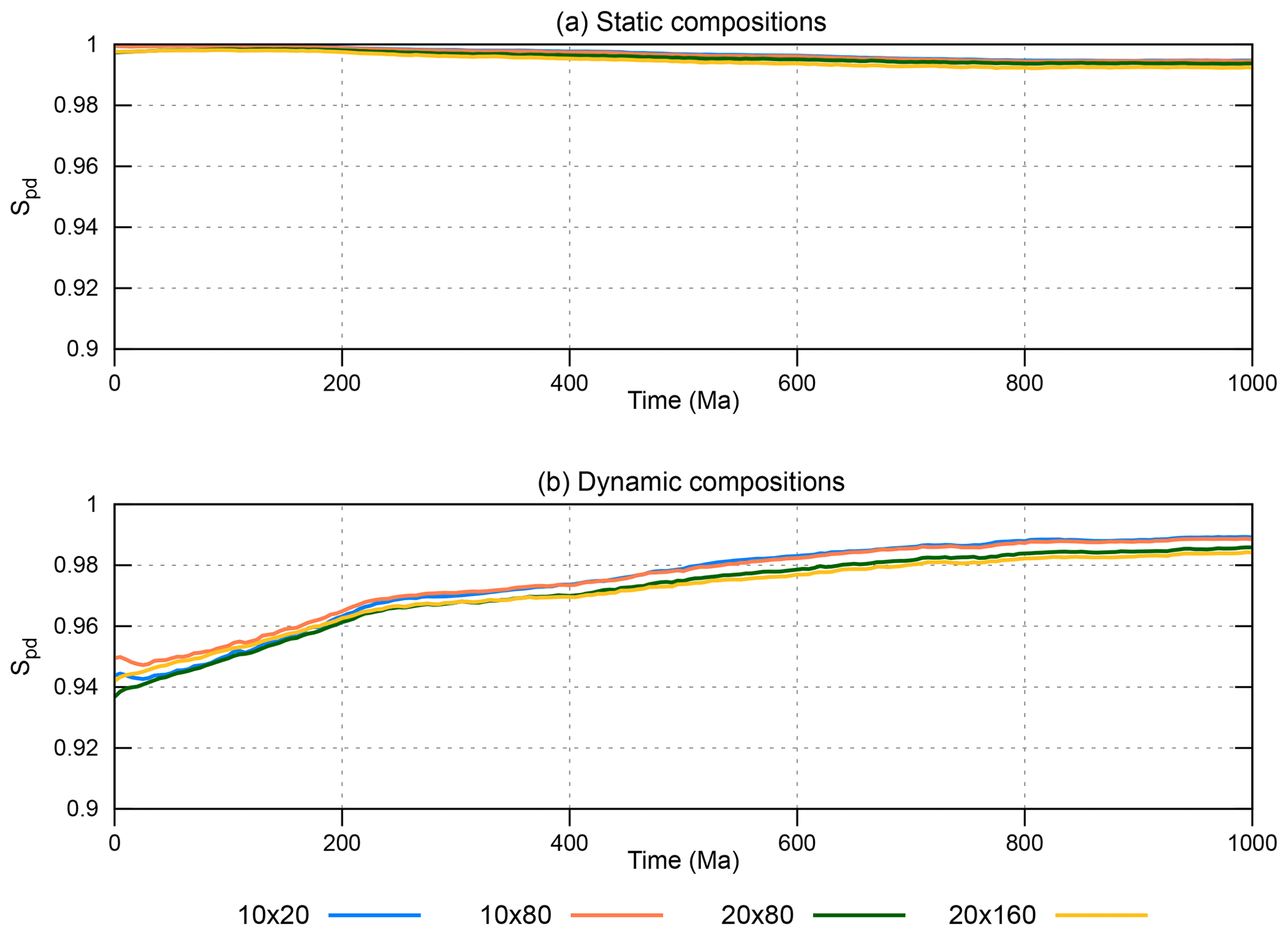
Figure 3Time evolution of Spd for the static (case A) and dynamic (case B) composition distributions of the four resolutions used.
3.1 Global particle distribution (Spd)
A total of ∼ 96 000 particles are initially distributed in a regular pattern (Fig. 2), equally spaced throughout the annulus. Over time, these particles are passively advected; thus their spatial distribution changes. The large number of particles in the initial distribution provides a good coverage in all cells as quantified by the normalized global entropy of particle distribution Spd, which is at the modelling start close to 1 for both cases A and B at the start (Fig. 3). As the initial composition ratios of case B are not equal (about 72 % lower mantle, 25 % upper mantle and 3 % lithosphere), Spd is not 1 as for case A but ∼ 0.95, still indicating that particles are distributed equally.
Over time, as particles are advected, the Spd does not change significantly for case A in which particles cannot change composition, but it does change for case B (Fig. 3). This is caused by the secular change in composition ratios in case B (Fig. A1 of van der Wiel et al., 2024). Spd increases due to the increased percentage of lithosphere and upper-mantle particles in the domain. We tested the effect of cell resolution on Spd for both cases, which does not show significant differences (Fig. 3). This indicates that the number of particles used in our calculations is sufficient, also for our highest resolution (20 × 160).
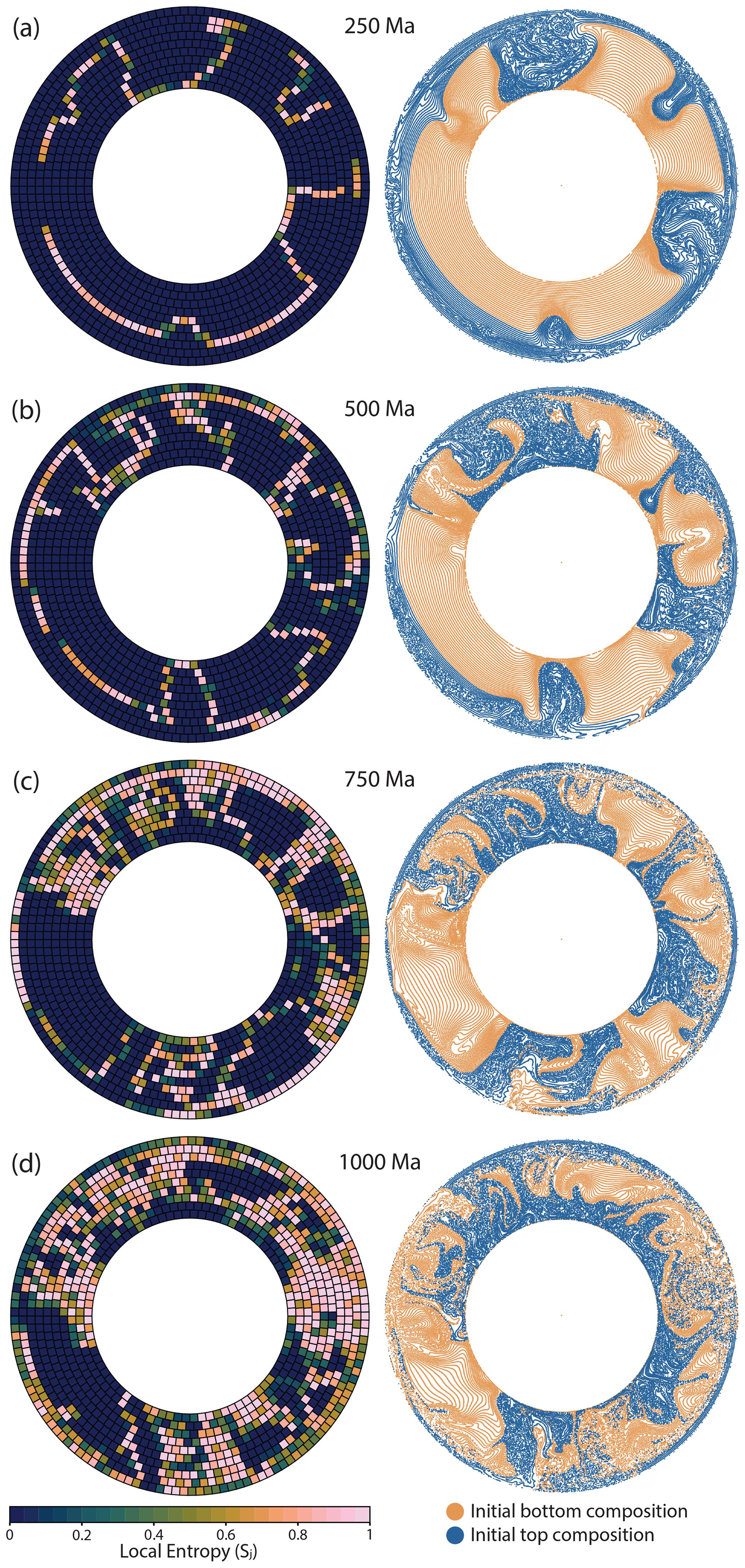
Figure 4Local entropy Sj (left) and particle distribution (right) at 250 Ma intervals of the model (model R; van der Wiel et al., 2024) with a static ratio particle composition (case A) at a resolution of 10 × 80 cells.
3.2 Local entropy (Sj)
A local entropy of 1 means that the ratio of particle compositions within a cell is equal to the global composition ratio, e.g. in the initial distribution for case A (Fig. 2). Sj=0 indicates that all particles in a cell have the same composition, although it does not indicate which composition. We illustrate the temporal evolution of particle distribution in 250 Ma steps (Fig. 4) for which we use the static particle composition ratio of case A and a cell resolution of 10 × 80 at the CMB (Fig. 3). After 250 Ma of convection evolution, the initial distribution is undisturbed in most parts of the domain. The two compositions are only displaced since the onset of convection, but they are barely mixed. Mixing is concentrated around two major zones of downwelling where a narrow zone of single cells shows a local entropy Sj that is non-zero (Fig. 4a).
At 500 Ma, some of the sharp boundaries between the two compositions have moved, and a mixed boundary zone has formed locally, reflected by the broader zone of non-zero local entropy (Fig. 4b). After 750 Ma, most of the upper mantle (top three cells) has Sj>0, and zones in the lower mantle are mixed as well (Fig. 4c): the two starting compositions have been displaced and mixed through the mantle. At the end of the model, at 1000 Ma, the number of cells with non-zero Sj in the upper mantle has decreased further, and the zones of fully (Sj≈1) mixed lower mantle have increased in area. However, there are still zones of unmixed (Sj=0) composition present. Unmixed initial “lower” composition is preserved mainly in the mid-mantle, while unmixed initial “upper” composition is preserved near the CMB; i.e., this material sunk and was displaced but did not mix (Fig. 4d).
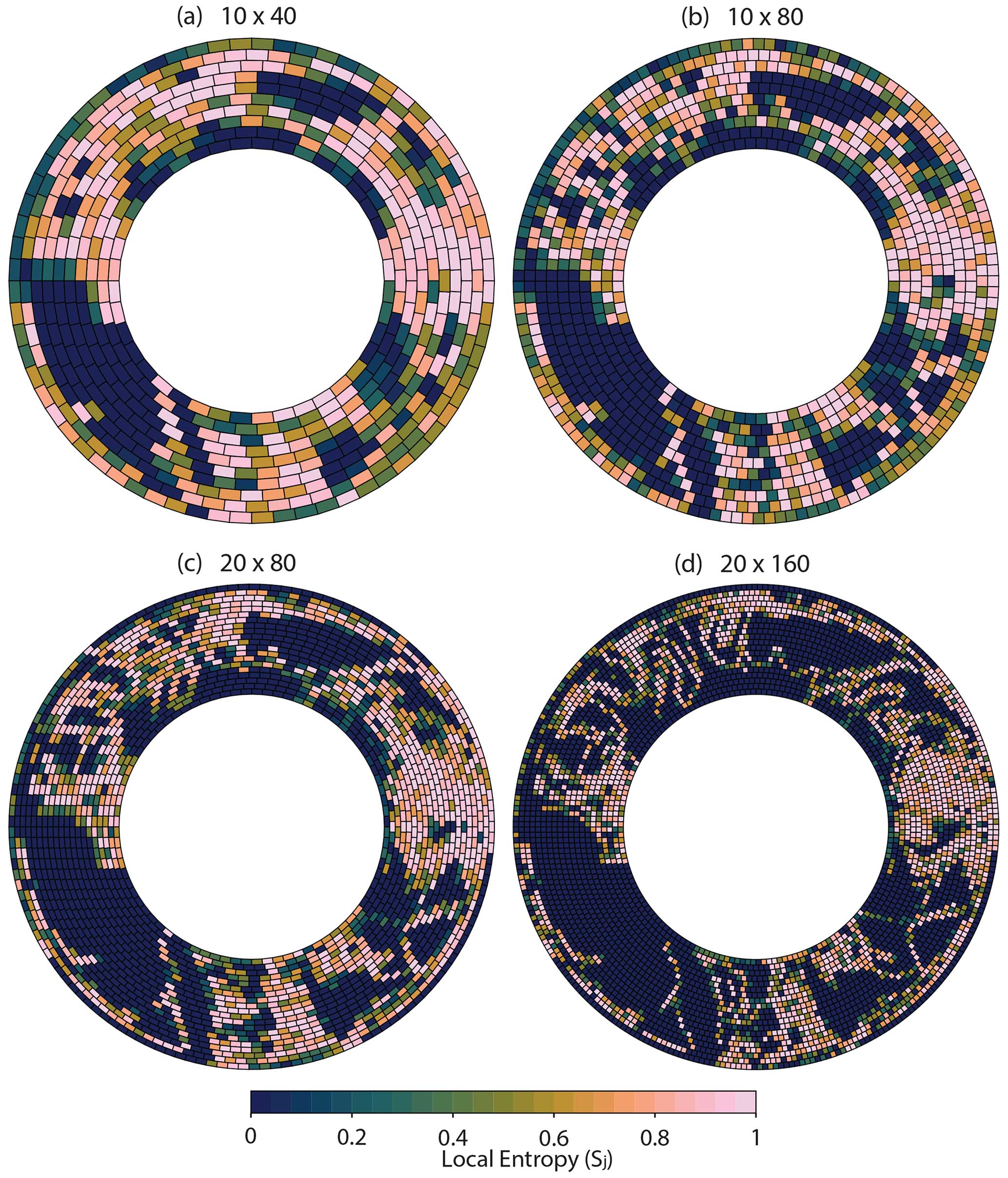
Figure 5Local entropy Sj after 1000 Ma of mantle convection for the reference model (van der Wiel et al., 2024) at four different resolutions of cells used to calculate the local entropy, where panel (b) is identical to Fig. 4d.
Even though cell resolution does not significantly impact Spd, it does affect the local entropy Sj (and thus also the global entropy; see next section). A smaller cell mesh will have fewer particles per cell, which increases the likelihood of sampling particles of only one composition in zones with limited mixing, leading to 0 local entropy. Doubling the angular resolution from 10 × 40 to 10 × 80 shows a similar trend on a global scale after 1000 Ma of convection: three zones of unmixed (low Sj) mantle separated by three zones of mixed (high Sj) mantle (Fig. 5). However, it does show some increased detail in local entropy, mainly in the “mixed” zones of the model (Fig. 5). The large unmixed zones are of similar size for these two resolutions, although the ratio of cells with a low Sj compared to a high Sj changed. The larger unmixed zones are composed of initial “lower” composition (Fig. 4d).
A radial increase in resolution, from 10 to 20 cells across the domain, refines the calculation of local entropy. The number of cells with Sj=0 becomes larger and increases the size of the three main unmixed zones. At this resolution, Sj resolves the “continents”: thicker portions of lithosphere that were initially placed in the model (see Fig. 2. of van der Wiel et al., 2024). The 20 × 80 resolution has unmixed cells in regions that had high Sj at lower resolutions (Fig. 5). Finally, with the 20 × 160 mesh resolution, zones of initial upper and lower composition (Fig. 4d) show up as low Sj bounded by a single line of cells with high Sj (Fig. 5). At this resolution the local entropy calculation resolves mantle structures such as the boundaries between slabs and ambient mantle, showing mantle structure mapped into the local entropy of mixing.
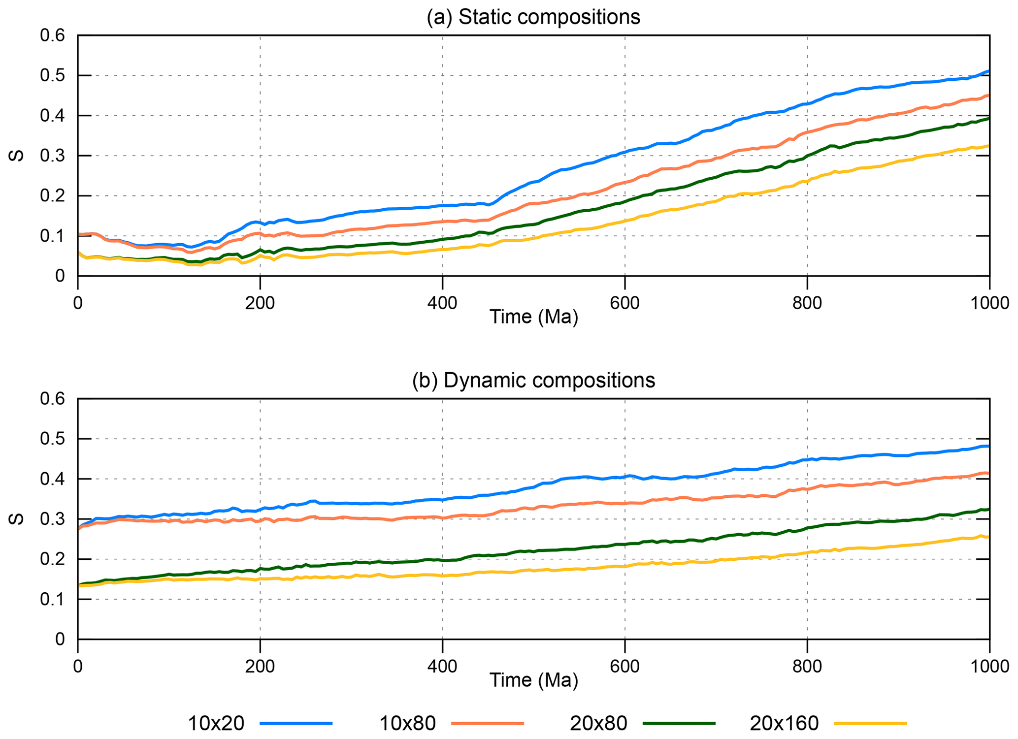
Figure 6Global entropy S of the model through time for different cell resolutions. (a) Case A (static compositions). (b) Case B (dynamic compositions).
3.3 Global entropy (S)
The global entropy is a weighted average of the particle distribution proportion Pj over cells and the compositional distribution within the cells Sj (Eq. 6). Because the particle distribution irrespective of composition is almost equal to 1 in all tests (Fig. 2, Sect. 3.1), we may regard the entropy S as a proxy for global compositional mixing. For the initial distribution of composition based on depth, almost all cells have a local entropy Sj=0, apart from the cells that straddle the compositional boundary (Fig. 2). This distribution is an unmixed state of the mantle and has a low global entropy, S=0.1 for the resolutions with 10 radial levels and S=0.06 for those with 20 radial levels (Fig. 6). The lateral resolution does not matter for the initial distribution, as the ratio of non-zero to zero Sj cells is the same.
While the mantle flow model evolves, compositions become more mixed and the global entropy increases depending on mesh resolution, whereby smaller cells have a higher chance to sample only one composition. Therefore, a higher resolution (smaller cells) yields a lower global entropy after 1000 Ma of mantle convection: the 20 × 160 resolution yields S=0.32, while the 10 × 40 resolution yields S=0.51 (Fig. 6).
3.4 Case study: entropy with dynamic compositions
Case B, which has dynamic compositions that depend on compositional evolution in the model, presents a practical application of the configurational entropy. We track the entropy as the compositional ratios evolve and mix over time. The total number of particles that have been part of the lithosphere and subducted increases over time as new lithosphere and slab are being created, while the volume of material that stays in the lower mantle decreases. In our example model, after 1000 Ma, the initial volumes of 3 % lithosphere, 25 % upper mantle and 72 % lower mantle have changed to 25 % with lithosphere “composition”, 50 % upper mantle and 25 % lower mantle. In this example, the dynamic composition implies that no lower-mantle composition exists above the 660 km discontinuity; therefore the upper mantle cannot have a local entropy of 1. However, in parts of the lower mantle, the three compositions are mixed where high local entropy is present. The parts of the domain containing subducted lithosphere are better mixed, indicative of the convective mixing behaviour of our model. With the highest mesh resolution, we can resolve the upper- to lower-mantle boundary in the local entropy and in active and past locations of subduction (Fig. 7a).
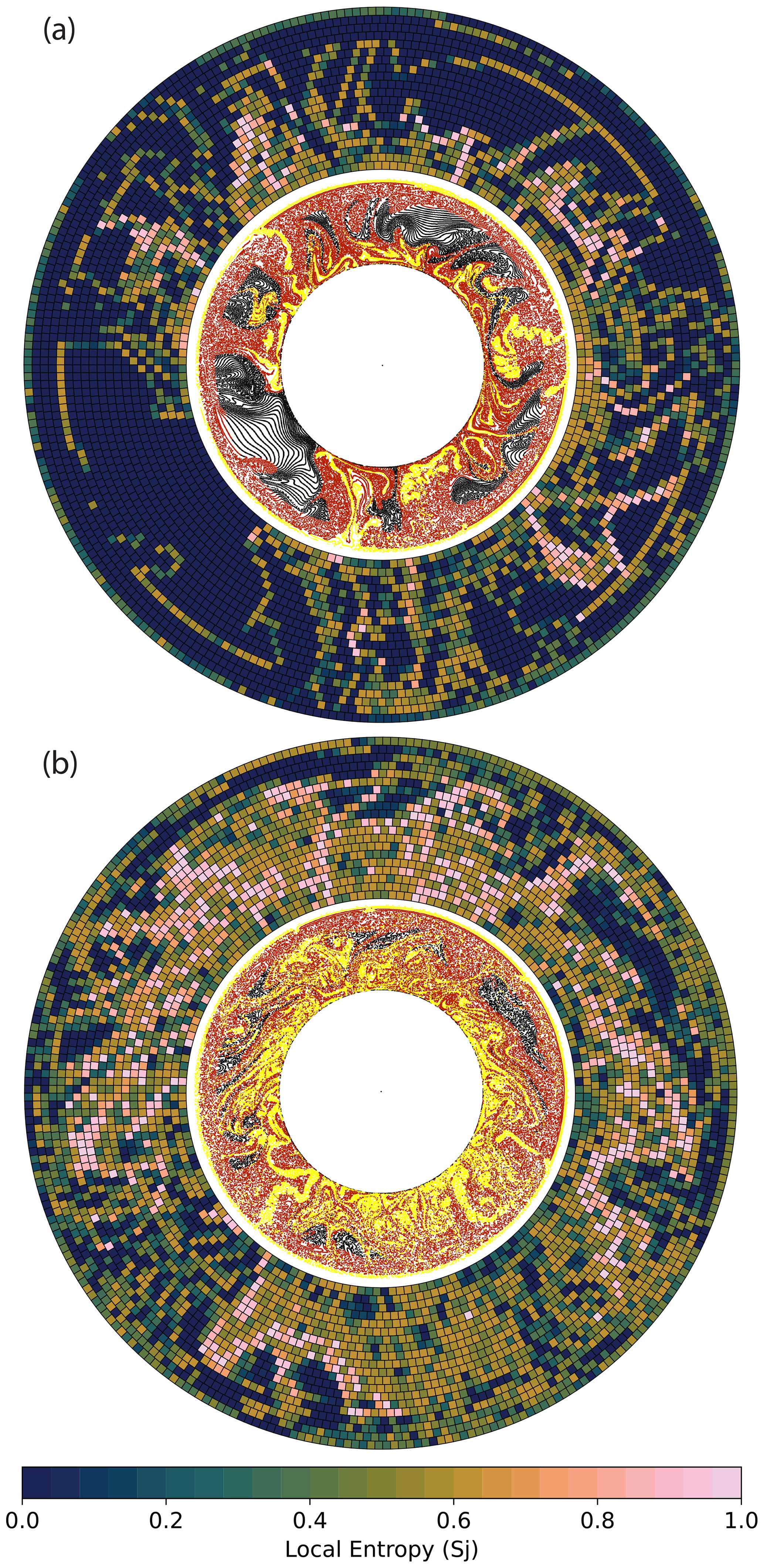
Figure 7Local entropy Sj with a 20 × 160 resolution (outer annulus) and particle distribution (inner annulus) for dynamic compositions after 1000 Ma of simulated convection. Lower-mantle (black), upper-mantle (red) and lithosphere (yellow) compositions can change over time as functions of depth. (a) Model R and (b) model P with a more vigorous convection of van der Wiel et al. (2024), as described in Sect. 3.4.
The unmixed zones are of particular interest, since they may provide direct information about compositions after 1000 Ma of convection. For all compositions there are cells with an unmixed signal, revealing the state of preservation of these compositions over time and over the whole domain. The entropy figures illustrate, for instance, the survival of unmixed original lower-mantle material in the model, the fate of subducted lithosphere and how upper-mantle material is entrained downward during subduction (Fig. 7a).
This case has an entirely different local entropy than the static composition distribution of case A (Fig. 5). The dynamic case mainly focuses on the fate of subducted lithosphere rather than global mixing of the upper and lower part of the domain. As in the example with a static composition (case A), the global entropy S for dynamic compositions is also cell-size-dependent. The initial global entropy is higher than for static compositions, as there are now two compositional boundaries, and over time the entropy only increases up to S=0.25 for the 20 × 160 resolution. For the 10 × 40 resolution, S=0.48 after 1000 Ma, which is in the same range as the static two-composition example (Fig. 6).
Finally, we use the dynamic composition to illustrate how changing the vigour of mantle convection changes the entropy. To this end, we compute the entropy after 1000 Ma using a model in which much higher sinking rates of subducted slabs occurred than inferred (model P; van der Wiel et al., 2024) and that consequently has faster mantle flow. Figure 7b illustrates that this model is much more mixed after 1000 Ma of convection than in model R (Fig. 7a). It has cells with a local entropy close to 1 throughout much of the domain, and unmixed zones are smaller and located only in the top of lower mantle. Most of the local entropies are in the mid-mixed range. This is because only 10 % of the original “lower-mantle” composition remains. Global entropy S equals 0.42 for this model at the 20 × 160 resolution, and even 0.60 for the 10 × 40 resolution, which is significantly higher than the reference model with dynamic composition (Fig. 6). This example illustrates that the configurational entropy is able to quantify mixing states in mantle convection models and is sensitive to overall changes in model behaviour.
In this paper, we explore how configurational entropy may be applied to mantle convection models to quantify the degree of mechanical mixing, both on a local and global scale. Our results illustrate that entropy provides a way to track or map compositional heterogeneity over time using tracers or particles, which are commonly available in geodynamical models. Depending on the complexity of numerical models, any information that is stored in these tracers can be used to differentiate between “compositions” used in the entropy calculations. The mantle convection models that we used to illustrate the use of configurational entropy were designed as numerical experiments to evaluate whether slab-sinking rates scale with the vigour of mantle convection and mixing, and they did not aim to make a direct comparison between the model and the real Earth. A direct comparison between configurational entropy and other measures used to quantify mixing, like the Lyapunov exponents (or time), is beyond the scope of this work. We see two arguments in favour of configurational entropy for specific uses: (1) its measurement does not require an integration over time, thereby providing instant values for local and global entropy, and (2) its flexibility, since the spatial distribution of any field carried by the particles, passive or active, such as chemical composition, water content, reached depth and temperature, can be quantified.
For models that do make comparisons with the Earth, i.e. those that are kinematically constrained by reconstructed plate motions and aim to resemble Earth-like features (e.g. Bull et al., 2014; Coltice and Shephard, 2018; Faccenna et al., 2013; Flament et al., 2022; Li et al., 2023; Lin et al., 2022), configurational entropy may serve as a means to quantify and map the degree of mixing of varying compositions, and hence to determine average cell composition, on a local, regional or a global scale. In such models the Lyapunov time would be useful to quantify the deformation, or stretching, in the overall mantle (e.g. Coltice, 2005; van Keken and Zhong, 1999) or to quantify uncertainties in twin experiments (e.g. Bello et al., 2014; Bocher et al., 2016).
On a global scale, such models (if run for 2–4 Ga) would, for instance, be able to track volumes of material that have remained in the lower mantle during the evolution of Earth (Fig. 7). These volumes are of interest because they could explain the geochemical detection of enigmatic primordial mantle and feature in numerical models as the proposed bridgmanite-enriched ancient mantle structures (BEAMS) of Ballmer et al. (2017), survive in the slab graveyard (Jones et al., 2021), or perhaps feature in LLSVPs or ULVZs (Deschamps et al., 2012; Flament et al., 2022; McNamara, 2019; Vilella et al., 2021). In addition, the use of entropy calculations may show how subducted lithosphere may become stored in the mantle and to what degree original depleted and enriched crust and slab material mix with upper- and lower-mantle rock. In particular, dynamically changing compositions would benefit such studies, and, in more sophisticated models that include geochemical evolution (e.g. Dannberg and Gassmöller, 2018; Gülcher et al., 2021), geochemical reservoirs can be quantified with configurational entropy.
At smaller scales, entropy in mantle modelling is useful to track mixing at the scale of a single subducting plate interacting with a mantle wedge or a plume rising from the CMB. This may be done based solely on location (Spd) to track the dispersal of an initial cloud of tracers in a slab or at the base of a plume (Naliboff and Kellogg, 2007) but also with the use of composition through Sj and S. For instance, it may quantify how different compositions of material from the lowermost mantle are entrained by a plume and how material entrained by that plume is mixed during its upward motion (e.g. Dannberg and Gassmöller, 2018). For instance, depending on how material is mixed in the partially melting plume head or in the partially melting upper mantle below a ridge, mixing on the scale of a magma chamber may also be mapped using configurational entropy (see Perugini et al., 2015).
However, it may not yet be possible to numerically represent 3D mixing and motion processes on all the scales illustrated above. In the end, the dynamics driving mantle convection may force slow consumption and mixing away from primordial mantle by producing lithosphere and plumes and mixing the geochemically segregated remains of these back into the mantle. These processes form the basis of the widely recognized but still enigmatic geochemical reservoirs that are thought to reside in the lower mantle, such as those of recycled continental crust (EM1, EM2), recycled oceanic crust (HIMU) (Yan et al., 2020), recycled depleted lithospheric mantle (Stracke et al., 2019) and remaining primordial mantle (Ballmer et al., 2017; Gülcher et al., 2020; Jackson et al., 2017). These processes also culminate in the seismologically imaged mantle volumes of higher and lower seismic velocity, or seismic attenuation, but the widely different scales at which geochemical and seismological observations are made pose a problem to link such observations. Numerical models may bridge these scales and eventually use our planet's plate tectonic evolution to predict the geochemical reservoirs as tapped by volcanoes and the mantle structure as imaged by seismology. The configurational entropy in this paper may be helpful to quantitatively determine where numerical models may successfully predict these seismological and geochemical features.
Here we recall the equations of the article and show the equations for normalization, where nc,j is the number of particles per composition c in a cell j and Nc is the total number of c particles divided by the number of cells M. C represents the number of compositions used.
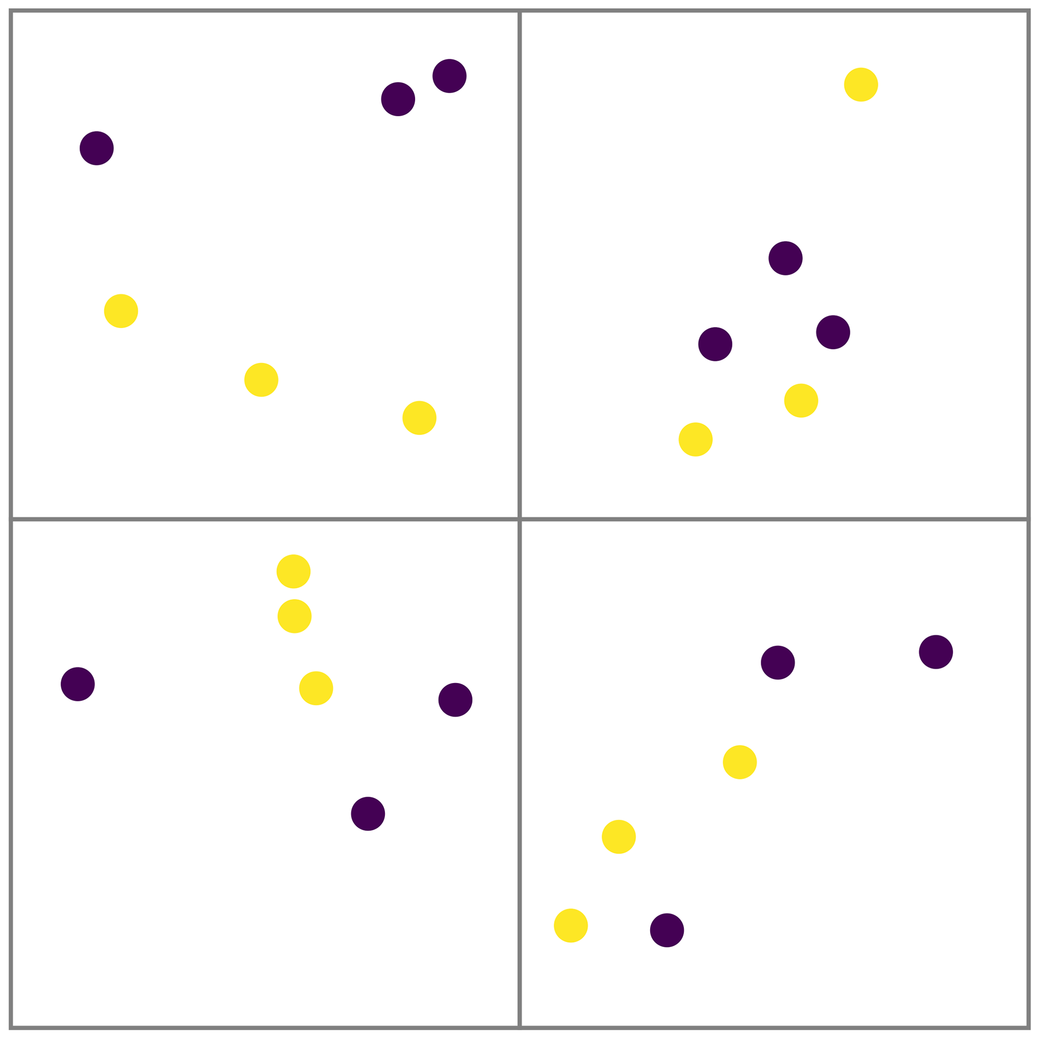
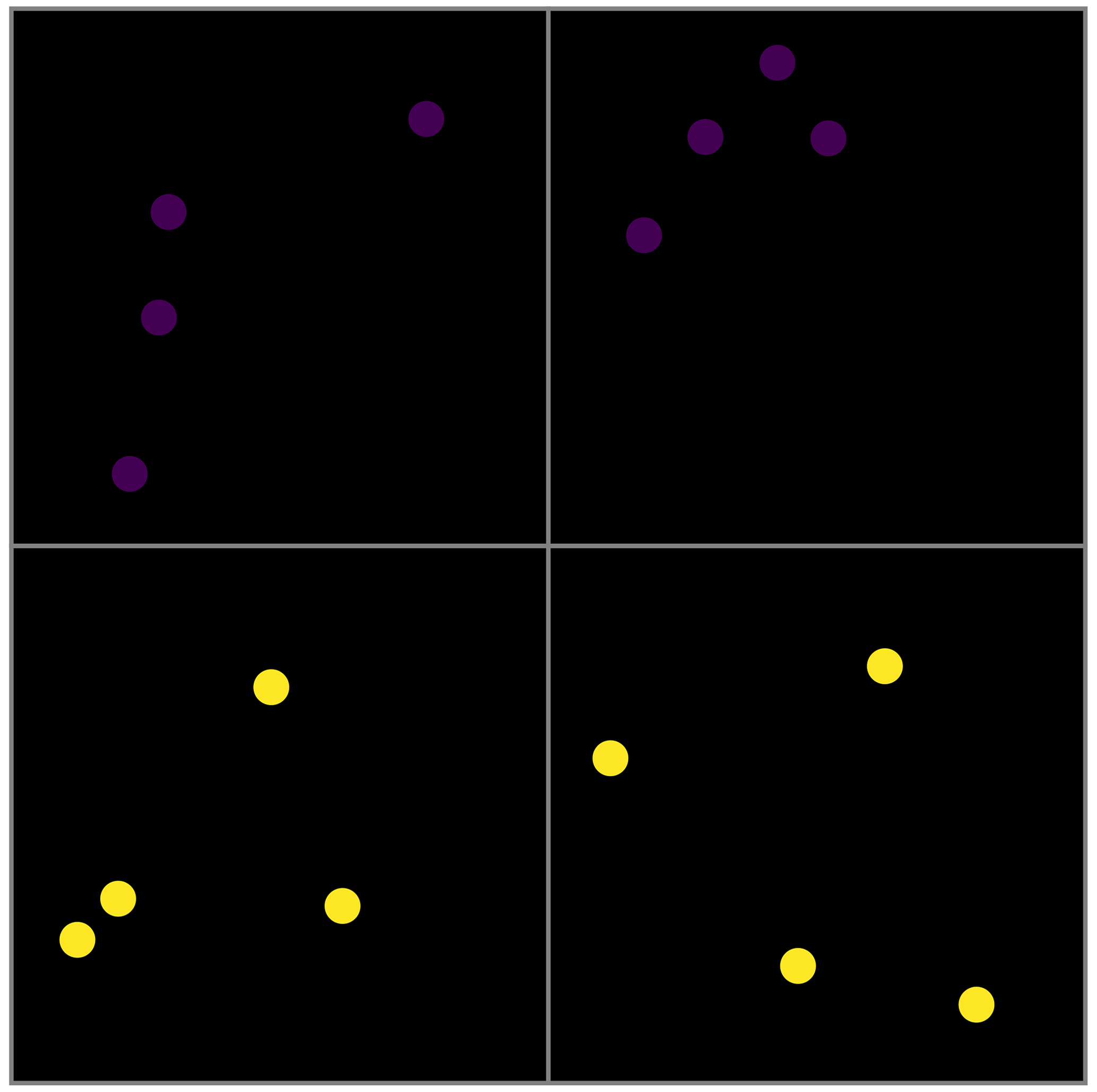
Four examples are given below, each with different distributions of particles and compositions in a small rectangular grid of four cells. We use these four examples to illustrate how the configurational entropy is affected by certain distributions. The background of each cell is coloured according to Sj in greyscale, from 0 (black) to 1 (white), and the tracers shown are randomly given a position in the cell appointed to them.
A1 Example 1: equal distribution, fully mixed
We start with a uniform distribution of particles with completely mixed compositions in each cell. The number of expected particles per composition per cell (Nc) is equal to the sum of the number of particles in that cell. This also reflected in vector Pj which is equal for all cells; therefore Spd is equal to 1 (after normalization), indicating a uniform distribution. The local entropy Sj per cell is defined through Pj,c, which is equally distributed and equal to the normalization. Therefore, it indicates perfect mixing for all four cells. The global entropy combines Pj and Sj and is therefore equal to the endmember, which is 1.
A2 Example 2: equal distribution, no mixing
The spatial distribution of particles is the same as in example 1, but compositions are not mixed, so Spd is still 1. Pj,c is either 1 or 0 per composition, with both leading to a 0 for the local entropy, which is therefore 0 for all four cells. As this local entropy feeds into the global entropy S, it is also 0.
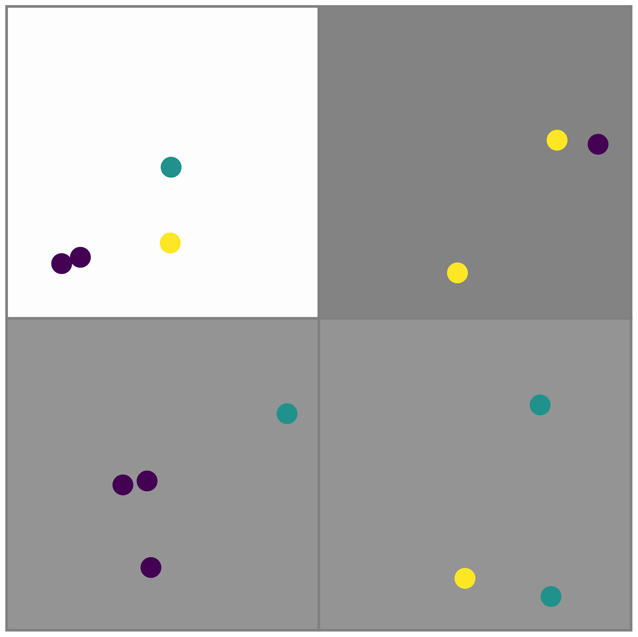
A3 Example 3: random example with three compositions
The distribution is ideally mixed, as the expected number of particles in each cell is 3.5. Pj is therefore not the same in each cell, but it is close to that. Spd is therefore close to 1 in this example. The compositions are not equally distributed: the top-left cell is close to the expected distribution (Nc) and therefore has a local entropy close to 1 (after normalization by ln (3)). The bottom cells are equally far off expected values (1.5 off for purple and 1 for the other colours) and therefore have the same Sj. As three cells have a local entropy of about 0.5 but distributions are somewhat equal, the global normalized entropy is 0.678 – this reflects the weighted average of Sj, which is the global entropy.
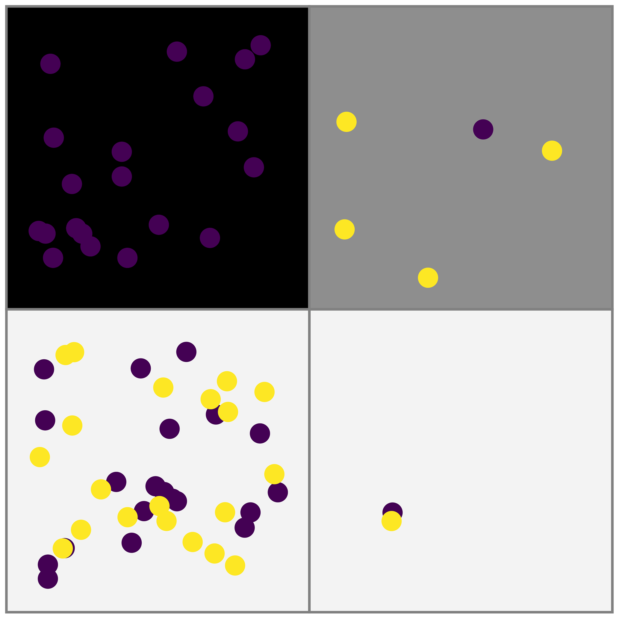
A4 Example 4: no equal distribution
This last case showcases an uneven particle distribution, with an expected number of particles of 16.75 (sum Nc) that is not recovered in any cell. The vector Pj is therefore not balanced, and Spd normalized is 0.689, indicating an imperfect particle distribution. The top left is obviously unmixed, with Sj=0. The bottom cells have the same ratio of compositions and therefore a similarly high Sj, as the compositional ratio is not too far off the ideal ratio. The bottom cells contribute significantly to the global entropy S, and the top left cell has a sizable weighing factor (P3=0.238), but as its Sj=0 it therefore does not contribute to the total entropy.
The code (Fieldstone 137) that was used to create the Appendix, which calculates all the appropriate values, can be found online at https://github.com/cedrict/fieldstone/blob/master/python_codes/fieldstone_137/ministone.py (Thieulot, 2024), or https://doi.org/10.5194/egusphere-egu23-14212 (Thieulot, 2023).
The data used to make the figures are available on Zenodo (https://doi.org/10.5281/zenodo.10077983, van der Wiel, 2023).
EvdW: conceptualization, methodology, investigation, writing (original draft) and visualization. CT: methodology and writing (review and editing). DJJvH: supervision and writing (review and editing).
The contact author has declared that none of the authors has any competing interests.
Publisher's note: Copernicus Publications remains neutral with regard to jurisdictional claims made in the text, published maps, institutional affiliations, or any other geographical representation in this paper. While Copernicus Publications makes every effort to include appropriate place names, the final responsibility lies with the authors.
We thank Wim Spakman for discussions and Nicolas Coltice and an anonymous reviewer for their thoughtful suggestions that improved the paper.
This research has been supported by the Aard- en Levenswetenschappen, Nederlandse Organisatie voor Wetenschappelijk Onderzoek (grant no. 865.17.001).
This paper was edited by Taras Gerya and reviewed by Nicolas Coltice and one anonymous referee.
Ballmer, M. D., Houser, C., Hernlund, J. W., Wentzcovitch, R. M., and Hirose, K.: Persistence of strong silica-enriched domains in the Earth's lower mantle, Nat. Geosci., 10, 236–240, https://doi.org/10.1038/NGEO2898, 2017.
Bello, L., Coltice, N., Rolf, T., and Tackley, P. J.: On the predictability limit of convection models of the Earth's mantle, Geochem. Geophy. Geosy., 15, 2319–2328, 2014.
Bocher, M., Coltice, N., Fournier, A., and Tackley, P. J.: A sequential data assimilation approach for the joint reconstruction of mantle convection and surface tectonics, Geophys. J. Int., 204, 200–214, 2016.
Bower, D. J., Gurnis, M., and Flament, N.: Assimilating lithosphere and slab history in 4-D Earth models, Phys. Earth Planet. In., 238, 8–22, https://doi.org/10.1016/j.pepi.2014.10.013, 2015.
Bull, A. L., Domeier, M., and Torsvik, T. H.: The effect of plate motion history on the longevity of deep mantle heterogeneities, Earth Planet. Sc. Lett., 401, 172–182, https://doi.org/10.1016/j.epsl.2014.06.008, 2014.
Camesasca, M., Kaufman, M., and Manas-Zloczower, I.: Quantifying fluid mixing with the Shannon entropy, Macromol. Theor. Simul., 15, 595–607, https://doi.org/10.1002/mats.200600037, 2006.
Christensen, U.: Mixing by time-dependent convection, Earth Planet. Sc. Lett., 95, 382–394, 1989.
Colli, L., Bunge, H. P., and Schuberth, B. S.: On retrodictions of global mantle flow with assimilated surface velocities, Geophys. Res. Lett., 42, 8341–8348, 2015.
Coltice, N.: The role of convective mixing in degassing the Earth's mantle, Earth Planet. Sc. Lett., 234, 15–25, 2005.
Coltice, N. and Schmalzl, J.: Mixing times in the mantle of the early Earth derived from 2-D and 3-D numerical simulations of convection, Geophys. Res. Lett., 33, L23304, https://doi.org/10.1029/2006GL027707, 2006.
Coltice, N. and Shephard, G. E.: Tectonic predictions with mantle convection model, Geophys. J. Int., 213, 16–29, https://doi.org/10.1093/gji/ggx531, 2018.
Dannberg, J. and Gassmöller, R.: Chemical trends in ocean islands explained by plume–slab interaction, P. Nat. Acad. Sci. USA, 115, 4351–4356, https://doi.org/10.1073/pnas.1714125115, 2018.
Deschamps, F., Cobden, L., and Tackley, P. J.: The primitive nature of large low shear-wave velocity provinces, Earth Planet. Sc. Lett., 349, 198–208, https://doi.org/10.1016/j.epsl.2012.07.012, 2012.
Domeier, M. and Torsvik, T. H.: Plate tectonics in the late Paleozoic, Geosci. Front., 5, 303–350, https://doi.org/10.1016/j.gsf.2014.01.002, 2014.
Doucet, L. S., Li, Z.-X., Gamal El Dien, H., Pourteau, A., Murphy, J. B., Collins, W. J., Mattielli, N., Olierook, H. K., Spencer, C. J., and Mitchell, R. N.: Distinct formation history for deep-mantle domains reflected in geochemical differences, Nat. Geosci., 13, 511–515, https://doi.org/10.1038/s41561-020-0599-9, 2020.
Dupré, B. and Allègre, C. J.: Pb–Sr isotope variation in Indian Ocean basalts and mixing phenomena, Nature, 303, 142–146, https://doi.org/10.1038/303142a0, 1983.
Faccenna, C., Becker, T. W., Conrad, C. P., and Husson, L.: Mountain building and mantle dynamics, Tectonics, 32, 80–93, https://doi.org/10.1029/2012TC003176, 2013.
Farnetani, C. G. and Samuel, H.: Lagrangian structures and stirring in the Earth's mantle, Earth Planet. Sc. Lett., 206, 335–348, 2003.
Farnetani, C. G., Legras, B., and Tackley, P. J.: Mixing and deformations in mantle plumes, Earth Planet. Sc. Lett., 196, 1–15, 2002.
Ferrachat, S. and Ricard, Y.: Regular vs. chaotic mantle mixing, Earth Planet. Sc. Lett., 155, 75–86, 1998.
Ferrachat, S. and Ricard, Y.: Mixing properties in the Earth's mantle: Effects of the viscosity stratification and of oceanic crust segregation, Geochem. Geophy. Geosy., 2, 2000GC000092, https://doi.org/10.1029/2000GC000092, 2001.
Flament, N., Bodur, Ö. F., Williams, S. E., and Merdith, A. S.: Assembly of the basal mantle structure beneath Africa, Nature, 603, 846–851, https://doi.org/10.1038/s41586-022-04538-y, 2022.
Garnero, E. J., McNamara, A. K., and Shim, S.-H.: Continent-sized anomalous zones with low seismic velocity at the base of Earth's mantle, Nat. Geosci., 9, 481–489, https://doi.org/10.1038/NGEO2733, 2016.
Gazel, E., Trela, J., Bizimis, M., Sobolev, A., Batanova, V., Class, C., and Jicha, B.: Long-lived source heterogeneities in the Galapagos mantle plume, Geochem. Geophy. Geosy., 19, 2764–2779, https://doi.org/10.1029/2017GC007338, 2018.
Gerya, T.: Precambrian geodynamics: concepts and models, Gondwana Res., 25, 442–463, https://doi.org/10.1016/j.gr.2012.11.008, 2014.
Goltz, C. and Böse, M.: Configurational entropy of critical earthquake populations, Geophys. Res. Lett., 29, 51-1–51-4, https://doi.org/10.1029/2002GL015540, 2002.
Gottschaldt, K.-D., Walzer, U., Hendel, R., Stegman, D. R., Baumgardner, J., and Mühlhaus, H.-B.: Stirring in 3-d spherical models of convection in the Earth's mantle, Phil. Mag., 86, 3175–3204, 2006.
Gülcher, A. J., Gebhardt, D. J., Ballmer, M. D., and Tackley, P. J.: Variable dynamic styles of primordial heterogeneity preservation in the Earth's lower mantle, Earth Planet. Sc. Lett., 536, 116160, https://doi.org/10.1016/j.epsl.2020.116160, 2020.
Gülcher, A. J. P., Ballmer, M. D., and Tackley, P. J.: Coupled dynamics and evolution of primordial and recycled heterogeneity in Earth's lower mantle, Solid Earth, 12, 2087–2107, https://doi.org/10.5194/se-12-2087-2021, 2021.
Gurnis, M. and Davies, G. F.: The effect of depth-dependent viscosity on convective mixing in the mantle and the possible survival of primitive mantle, Geophys. Res. Lett., 13, 541–544, 1986a.
Gurnis, M. and Davies, G. F.: Mixing in numerical models of mantle convection incorporating plate kinematics, J. Geophys. Res.-Sol. Ea., 91, 6375–6395, 1986b.
Hart, S. R.: A large-scale isotope anomaly in the Southern Hemisphere mantle, Nature, 309, 753–757, https://doi.org/10.1038/309753a0, 1984.
Heister, T., Dannberg, J., Gassmöller, R., and Bangerth, W.: High accuracy mantle convection simulation through modern numerical methods – II: realistic models and problems, Geophys. J. Int., 210, 833–851, https://doi.org/10.1093/gji/ggx195, 2017.
Hoernle, K., Werner, R., Morgan, J. P., Garbe-Schönberg, D., Bryce, J., and Mrazek, J.: Existence of complex spatial zonation in the Galápagos plume, Geology, 28, 435–438, https://doi.org/10.1130/0091-7613(2000)28<435:EOCSZI>2.0.CO;2, 2000.
Hoffman, N. and McKenzie, D.: The destruction of geochemical heterogeneities by differential fluid motions during mantle convection, Geophys. J. Int., 82, 163–206, 1985.
Homrighausen, S., Hoernle, K., Hauff, F., Hoyer, P. A., Haase, K. M., Geissler, W. H., and Geldmacher, J.: Evidence for compositionally distinct upper mantle plumelets since the early history of the Tristan-Gough hotspot, Nat. Commun., 14, 3908, https://doi.org/10.1038/s41467-023-39585-0, 2023.
Hunt, D. and Kellogg, L.: Quantifying mixing and age variations of heterogeneities in models of mantle convection: Role of depth-dependent viscosity, J. Geophys. Res.-Sol. Ea., 106, 6747–6759, 2001.
Jackson, M. and Macdonald, F.: Hemispheric geochemical dichotomy of the mantle is a legacy of austral supercontinent assembly and onset of deep continental crust subduction, AGU Adv., 3, e2022AV000664, https://doi.org/10.1029/2022AV000664, 2022.
Jackson, M., Konter, J., and Becker, T.: Primordial helium entrained by the hottest mantle plumes, Nature, 542, 340–343, https://doi.org/10.1038/nature21023, 2017.
Jackson, M., Becker, T., and Konter, J.: Evidence for a deep mantle source for EM and HIMU domains from integrated geochemical and geophysical constraints, Earth Planet. Sc. Lett., 484, 154–167, https://doi.org/10.1016/j.epsl.2017.11.052, 2018.
Jones, T. D., Sime, N., and van Keken, P.: Burying Earth's primitive mantle in the slab graveyard, Geochem. Geophy. Geosy., 22, e2020GC009396, https://doi.org/10.1029/2020GC009396, 2021.
Kellogg, L. and Turcotte, D.: Mixing and the distribution of heterogeneities in a chaotically convecting mantle, J. Geophys. Res.-Sol. Ea., 95, 421–432, https://doi.org/10.1029/JB095iB01p00421, 1990.
Kellogg, L. H.: Chaotic mixing in the Earth's mantle, Adv. Geophys., 34, 1–33, 1993.
Koelemeijer, P., Deuss, A., and Ritsema, J.: Density structure of Earth's lowermost mantle from Stoneley mode splitting observation, Nat. Commun., 8, 1–10, https://doi.org/10.1038/ncomms15241, 2017.
Li, Y., Liu, L., Peng, D., Dong, H., and Li, S.: Evaluating tomotectonic plate reconstructions using geodynamic models with data assimilation, the case for North America, Earth Sci. Rev., 244, 104518, https://doi.org/10.1016/j.earscirev.2023.104518, 2023.
Lin, Y. A., Colli, L., and Wu, J.: NW Pacific-Panthalassa intra-oceanic subduction during Mesozoic times from mantle convection and geoid models, Geochem. Geophy. Geosy., 23, e2022GC010514, https://doi.org/10.1029/2022GC010514, 2022.
McNamara, A. K.: A review of large low shear velocity provinces and ultra low velocity zones, Tectonophysics, 760, 199–220, https://doi.org/10.1016/j.tecto.2018.04.015, 2019.
Merdith, A. S., Williams, S. E., Collins, A. S., Tetley, M. G., Mulder, J. A., Blades, M. L., Young, A., Armistead, S. E., Cannon, J., and Zahirovic, S.: Extending full-plate tectonic models into deep time: Linking the Neoproterozoic and the Phanerozoic, Earth Sci. Rev., 214, 103477, https://doi.org/10.1016/j.earscirev.2020.103477, 2021.
Naliboff, J. B. and Kellogg, L. H.: Can large increases in viscosity and thermal conductivity preserve large-scale heterogeneity in the mantle?, Phys. Earth Planet. In., 161, 86–102, https://doi.org/10.1016/j.pepi.2007.01.009, 2007.
Olson, P., Yuen, D. A., and Balsiger, D.: Convective mixing and the fine structure of mantle heterogeneity, Phys. Earth Planet. In., 36, 291–304, 1984a.
Olson, P., Yuen, D. A., and Balsiger, D.: Mixing of passive heterogeneities by mantle convection, J. Geophys. Res.-Sol. Ea., 89, 425–436, 1984b.
Perugini, D., De Campos, C., Petrelli, M., Morgavi, D., Vetere, F. P., and Dingwell, D.: Quantifying magma mixing with the Shannon entropy: Application to simulations and experiments, Lithos, 236, 299–310, https://doi.org/10.1016/j.lithos.2015.09.008, 2015.
Richter, F. M., Daly, S. F., and Nataf, H.-C.: A parameterized model for the evolution of isotopic heterogeneities in a convecting system, Earth Planet. Sc. Lett., 60, 178–194, 1982.
Ritsema, J. and Lekić, V.: Heterogeneity of seismic wave velocity in Earth's mantle, Annu. Rev. Earth Pl. Sc., 48, 377–401, https://doi.org/10.1146/annurev-earth-082119-065909, 2020.
Ritsema, J., Deuss, A., Van Heijst, H., and Woodhouse, J.: S40RTS: a degree-40 shear-velocity model for the mantle from new Rayleigh wave dispersion, teleseismic traveltime and normal-mode splitting function measurements, Geophys. J. Int., 184, 1223–1236, https://doi.org/10.1111/j.1365-246X.2010.04884.x, 2011.
Samuel, H., Aleksandrov, V., and Deo, B.: The effect of continents on mantle convective stirring, Geophys. Res. Lett., 38, L04307, https://doi.org/10.1029/2010GL046056, 2011.
Schmalzl, J., Houseman, G., and Hansen, U.: Mixing in vigorous, time-dependent three-dimensional convection and application to Earth's mantle, J. Geophys. Res.-Sol. Ea., 101, 21847–21858, 1996.
Shannon, C. E.: A mathematical theory of communication, Bell Syst. Tech. J., 27, 379–423, https://doi.org/10.1002/j.1538-7305.1948.tb01338.x, 1948.
Stegman, D. R., Richards, M. A., and Baumgardner, J. R.: Effects of depth-dependent viscosity and plate motions on maintaining a relatively uniform mid-ocean ridge basalt reservoir in whole mantle flow, J. Geophys. Res.-Sol. Ea., 107, ETG 5-1–ETG 5-8, 2002.
Stracke, A., Genske, F., Berndt, J., and Koornneef, J. M.: Ubiquitous ultra-depleted domains in Earth's mantle, Nat. Geosci., 12, 851–855, https://doi.org/10.1038/s41561-019-0446-z, 2019.
Tackley, P. J. and Xie, S.: The thermochemical structure and evolution of Earth's mantle: constraints and numerical models, Philos. T. Roy. Soc. A, 360, 2593–2609, 2002.
Ten, A. A., Podladchikov, Y. Y., Yuen, D. A., Larsen, T. B., and Malevsky, A. V.: Comparison of mixing properties in convection with the Particle-Line Method, Geophys. Res. Lett., 25, 3205–3208, 1998.
Thieulot, C.: GHOST: Geoscientific Hollow Sphere Tessellation, Solid Earth, 9, 1169–1177, https://doi.org/10.5194/se-9-1169-2018, 2018.
Thieulot, C.: FIELDSTONE: a computational geodynamics (self-)teaching tool, EGU General Assembly 2023, Vienna, Austria, 24–28 April 2023, EGU23-14212, https://doi.org/10.5194/egusphere-egu23-14212, 2023.
Thieulot, C.: Fieldstone, GitHub [code], https://github.com/cedrict/fieldstone/blob/master/python_codes/fieldstone_137/ministone.py (lat access: 7 November 2023), 2024.
Thomas, B., Samuel, H., Farnetani, C., Aubert, J., and Chauvel, C.: Mixing time of heterogeneities in a buoyancy-dominated magma ocean, Geophys. J. Int., 236, 764–777, 2024.
van der Meer, D. G., van Hinsbergen, D. J. J., and Spakman, W.: Atlas of the underworld: Slab remnants in the mantle, their sinking history and a new outlook on lower mantle viscosity, Tectonophysics, 723, 309–448, https://doi.org/10.1016/j.tecto.2017.10.004, 2018.
van der Wiel, E.: Data for: Quantifying mantle mixing through Configurational Entopy [Data set], Zenodo [data set], https://doi.org/10.5281/zenodo.10077983, 2023.
van der Wiel, E., van Hinsbergen, D. J., Thieulot, C., and Spakman, W.: Linking rates of slab sinking to long-term lower mantle flow and mixing, Earth Planet. Sc. Lett., 625, 118471, https://doi.org/10.1016/j.epsl.2023.118471, 2024.
van Keken, P. and Zhong, S.: Mixing in a 3D spherical model of present-day mantle convection, Earth Planet. Sc. Lett., 171, 533–547, 1999.
van Keken, P. E., Ballentine, C. J., and Hauri, E. H.: Convective mixing in the Earth's mantle, Treat. Geochem., 2, 1–21, 2003.
Vilella, K., Bodin, T., Boukaré, C.-E., Deschamps, F., Badro, J., Ballmer, M. D., and Li, Y.: Constraints on the composition and temperature of LLSVPs from seismic properties of lower mantle minerals, Earth Planet. Sc. Lett., 554, 116685, https://doi.org/10.1016/j.epsl.2020.116685, 2021.
Weis, D., Garcia, M. O., Rhodes, J. M., Jellinek, M., and Scoates, J. S.: Role of the deep mantle in generating the compositional asymmetry of the Hawaiian mantle plume, Nat. Geosci., 4, 831–838, https://doi.org/10.1038/ngeo1328, 2011.
Wellmann, J. F. and Regenauer-Lieb, K.: Uncertainties have a meaning: Information entropy as a quality measure for 3-D geological models, Tectonophysics, 526, 207–216, https://doi.org/10.1016/j.tecto.2011.05.001, 2012.
Wichmann, D., Delandmeter, P., Dijkstra, H. A., and van Sebille, E.: Mixing of passive tracers at the ocean surface and its implications for plastic transport modelling, Environ. Res. Commun., 1, 115001, https://doi.org/10.1088/2515-7620/ab4e77, 2019.
Yan, J., Ballmer, M. D., and Tackley, P. J.: The evolution and distribution of recycled oceanic crust in the Earth's mantle: Insight from geodynamic models, Earth Planet. Sc. Lett., 537, 116171, https://doi.org/10.1016/j.epsl.2020.116171, 2020.
Zahirovic, S., Müller, R. D., Seton, M., and Flament, N.: Tectonic speed limits from plate kinematic reconstructions, Earth Planet. Sc. Lett., 418, 40–52, https://doi.org/10.1016/j.epsl.2015.02.037, 2015.
configurational entropy, which allows us to quantify mixing in models. The entropy may be used to analyse the mixed state of the mantle as a whole and may also be useful to validate numerical models against anomalies in the mantle that are obtained from seismology and geochemistry.