What does it take to restore geological models with “natural” boundary conditions?

Structural restoration is commonly used to assess the deformation of geological structures and to reconstruct past basin geometries. Classically, restoration is formulated as a geometric or mechanical problem driven by geometric boundary conditions to flatten the top surface. This paper investigates the use of boundary conditions in restoration to better approach the actual mechanical processes driving geological deformations. For this, we use a reverse-time Stokes-based method with negative time step advection. To be able to compare the results of the restoration to known states of the model, we apply it to a model based on a laboratory analog experiment. In the study, we first test the behavior of the restoration process with Dirichlet boundary conditions such as those often used in geomechanical restoration schemes. To go further, we then relax these boundary conditions by removing direct constraints on velocity and replace them with more “natural” conditions such as Neumann and free-surface conditions. The horizontality of the free surface can then be measured and used as a restoration criterion instead of an imposed condition. The proposed boundary conditions result in a larger impact of the material properties on the restoration results. We then show that the choice of appropriate effective material properties is, therefore, necessary to restore structural models without kinematic boundary conditions.

1 Introduction

When studying the subsurface, geologists are faced with the sparsity of available data and need to make assumptions based on their knowledge to fill the gaps between the observations. Structural restoration, which aims at reversing tectonic deformations, was first introduced as a method to balance cross-sections and characterize shortening, allowing for the verification of these assumptions to some extent (e.g., Chamberlin, 1910; Dahlstrom, 1969; Schönborn, 1999). More recently, the approach has evolved to assess tectonic evolution through time (e.g., Back et al., 2008; de Melo Garcia et al., 2012; Espurt et al., 2019; Crook et al., 2018) or to assess the localization of deformation (e.g., Al-Fahmi et al., 2016; Chauvin et al., 2018). Various methods were developed to add more complexity and study different geological and physical aspects, such as erosion and deposition of sediments (e.g., Dimakis et al., 1998), isostasy compensation (e.g., Allen and Allen, 2013), thermal subsidence due to the mantle thermal effect (Royden and Keen, 1980; Allen and Allen, 2013), rock decompaction due to a change of load (e.g., Athy, 1930; Durand-Riard et al., 2011; Allen and Allen, 2013), or, at a smaller scale, the erosion and deposition of channelized systems (e.g., Parquer et al., 2017). In this article, we focus on structural restoration aiming at unfolding and unfaulting.

Various numerical methods have been developed for structural restoration, each using different deformation mechanisms. The first implementations used geometric and kinematic rules (e.g., Chamberlin, 1910; Dahlstrom, 1969; Gratier, 1988; Rouby, 1994; Groshong, 2006; Lovely et al., 2018; Fossen, 2016). Numerous authors, however, stressed their lack of physical principles and their limitations, for example in cases such as salt basins (Fletcher and Pollard, 1999; Ismail-Zadeh et al., 2001; Muron, 2005; Maerten and Maerten, 2006; Moretti, 2008; Guzofski et al., 2009; Al-Fahmi et al., 2016). Methods using geomechanical simulations were then developed, taking into account the material behavior inside the geological layers and applying a set of conditions to restore the models. In this approach, internal deformation is not known a priori; it is determined from the input mechanical behavior of rocks and the applied boundary conditions. For example, in the presence of salt structures, methods based on considering the rocks to be viscous fluids were introduced (Kaus and Podladchikov, 2001; Ismail-Zadeh et al., 2001, 2004; Ismail-Zadeh and Tackley, 2010). In these methods, the motion is computed using highly viscous fluid mechanical laws inside the stratigraphic units and their behavior under their own weight. This is motivated by the fact that rock salt and some sediment overburdens behave as viscous fluids over timescales of millions of years and by the reversibility of the Stokes equations. At this point, however, faults have been neglected in most of these restoration methods, except some numerical test cases (e.g., Schuh-Senlis et al., 2020). Many authors have also proposed using linear elastic behavior and frictionless faults (Maerten and Maerten, 2001; De Santi et al., 2002; Muron, 2005; Moretti et al., 2006; Maerten and Maerten, 2006; Guzofski et al., 2009; Durand-Riard et al., 2010, 2013a, b; Tang et al., 2016; Chauvin et al., 2018). These elastic restoration methods classically rely on boundary conditions that make the uppermost horizon flat, horizontal, and unfaulted at deposition time. The issue here is that while geological assumptions can give an idea of the total displacement that should happen, its discretization in time is unknown. As such, the validity and the ability of these boundary conditions to replace the tectonic forces applied to forward geologic deformation have been questioned (e.g., Lovely et al., 2012; Chauvin et al., 2018). In particular, Chauvin et al. (2018) show that a lateral kinematic boundary condition can be required for increasing the accuracy of elastic restoration. Schuh-Senlis et al. (2020) show the possible extension of the viscous fluid restoration method to sedimentary basins including faults and using less constraining boundary conditions, relying on a free surface (with no condition enforced on it) on top and the weight of the materials to drive the restoration process. However, the process was only tested by successively applying a forward and a backward simulation to synthetic models using the same software, physical laws, and material parameters.

In this paper, we investigate the complexity of restoring a more complex structural model obtained from an analog, gravity-driven laboratory experiment, without imposing any boundary condition on the free surface. In this approach, the free-surface horizontality will not be imposed but used as a criterion to check the restoration quality. We build on the method of Schuh-Senlis et al. (2020) and use the same creeping flow restoration process. The simulations done in this article also use the particle-in-cell implementation in the FAIStokes¹ code of Schuh-Senlis et al. (2020), for which key points are specified in Sect. 2.2. Creeping flow restoration is chosen here for three main reasons. First, the deformation inside the model is driven by gravity and backward time stepping. Second, it can handle the rheology of viscous layers (such as salt layers in geological models). Third, it allows the faults to be considered shear bands with a lower viscosity instead of frictionless surfaces.

To increase the knowledge on the previous states of the restored model and be able to compare the restoration results with these states, we use an analog experiment model as a test case. The purpose of analog modeling is, with forward experiments, to find the paleo-deformations leading to specific geological structures (Hall, 1815; Ramberg, 1981; Willis, 1894; Cobbold et al., 1989). The idea is to choose materials that present the same deformations as those observed in geological models but are sufficiently weak to deform at laboratory scales. For example, the experiment presented in this study has a size around 30 cm×5 cm and lasts about 3 h, but the properties of its materials are such that its deformation is similar to that of a sedimentary basin several kilometers wide over several hundreds of thousands of years. As a result, analog experiments produce structural models where not only the post-deformation state but also the paleo-state and the deformations undergone by the model are known. For this reason, several studies have used them to assess the results of numerical schemes, both forward (e.g., Buiter et al., 2016; Schreurs et al., 2016) and backward (e.g., Chauvin et al., 2018).

The outline of this paper is as follows: in Sect. 2 we review the concepts of Stokes-flow-based restoration and the FAIStokes implementation used in this study. In Sect. 3, we present the analog experiment which was used and the numerical model created from it. In Sect. 4, we start by restoring this model using boundary conditions which impose the deformation of the model and then replace them one by one to remove the kinematic dependance. For this, we introduce lateral boundary conditions which aim at better approaching the local stress state and remove the boundary condition on the top surface to leave it free. These boundary conditions, however, stress the importance of the material properties in the model and the inability of the method to restore the model properly without proper effective material properties. In Sect. 5 the last part, we show how the proposed boundary conditions could be used to assess the impact of the material parameters on the restoration and how to find relevant values for them.

2 Method

2.1 Creeping flow restoration

2.1.1 Stokes flow equations

In sedimentary basins, the deformation of rocks over long periods of time can be modeled by viscous fluids, for which the deformation is described by the Navier–Stokes equations. In this case, however, we usually deal with materials that are highly viscous (with a viscosity η over 10¹⁷ Pa s) over timescales of thousands to millions of years. The inertial part of the Navier–Stokes equations can then be neglected, and the deformation is described by the Stokes equations for creeping flow (Massimi et al., 2006). These equations consist of the momentum conservation equation,

$$\begin{array}{}\text{(1)}& \mathbf{\nabla }\cdot \mathit{\sigma }+\mathit{f}=\mathbf{0},\end{array}$$

where ∇ is the del operator, σ is the stress tensor, and f is the specific body force (usually the volumetric weight ρg), as well as the mass conservation equation for incompressible fluids (continuity equation),

$$\begin{array}{}\text{(2)}& \mathbf{\nabla }\cdot \mathit{v}=\mathrm{0},\end{array}$$

where v is the velocity. The stress consists of a deviatoric part τ and an isotropic pressure p:

$$\begin{array}{}\text{(3)}& \mathit{\sigma }=\mathit{\tau }-p\mathbf{I},\end{array}$$

where I is the identity tensor. In the viscous flow assumption, the deviatoric part of the stress is

$$\begin{array}{}\text{(4)}& \mathit{\tau }=\mathrm{2}\mathit{\eta }\mathbf{D},\end{array}$$

with η the dynamic viscosity and D the infinitesimal strain rate tensor defined by

$$\begin{array}{}\text{(5)}& \mathbf{D}={\displaystyle \frac{\mathrm{1}}{\mathrm{2}}}[\mathbf{\nabla }\mathit{v}+(\mathbf{\nabla }\mathit{v}{)}^T].\end{array}$$

Assembling Eqs. (1), (3), (4), and (5), the momentum conservation equation can be written as

$$\begin{array}{}\text{(6)}& \mathbf{\nabla }\cdot \left[\mathit{\eta }\right(\mathbf{\nabla }\mathit{v}+\left(\mathbf{\nabla }\mathit{v}{)}^T\right)]-\mathbf{\nabla }p=-\mathit{\rho }\mathit{g}.\end{array}$$

These equations describe a steady-state flow and their resolution provides the velocity of a fluid at a specific position and time. When different fluids are present, the conditions that are applied at their boundaries, as well as their differences in density, can create instabilities such as Rayleigh–Taylor instabilities. These instabilities make the flow nonstationary as they advect the viscosity and density fields in time.

2.1.2 Backward advection

In forward simulation schemes, the Stokes equations (Eqs. 6 and 2) are solved for pressure and velocity, and the material representation of the geological model is advected from the velocity at each time step. The simplest way to do it is by using an Euler scheme, the position x(t+Δt) of a given point of the material model after a single time step being computed as

$$\begin{array}{}\text{(7)}& \mathit{x}(t+\mathrm{\Delta }t)=\mathit{x}\left(t\right)+\mathit{v}\left(t\right)\cdot \mathrm{\Delta }t,\end{array}$$

where v(t) is the computed velocity of the point at time t. While higher-order methods exist (e.g., Ismail-Zadeh and Tackley, 2010), particularly to stabilize the advection scheme in the case of large time steps, we choose to present the restoration idea with this order 1 approximation for simplicity. This finite-difference approximation relies on the idea that the chosen time step Δt is small enough to approximate the velocity of a particle as a constant over this time step (Δt is usually calculated using a Courant–Friedrichs–Lewy – or CFL – condition; Courant et al., 1928). Since the Stokes equations are linear and do not depend on previous time steps for the computation of the velocity, we can extend this approximation to backward simulations. Instead of applying Eq. (7), we can apply

$$\begin{array}{}\text{(8)}& \mathit{x}(t-\mathrm{\Delta }t)=\mathit{x}\left(t\right)-\mathit{v}\left(t\right)\cdot \mathrm{\Delta }t\end{array}$$

for the advection of the points of the material model at each time step, like in Fig. 1. This is the basis of backward time stepping restoration schemes.

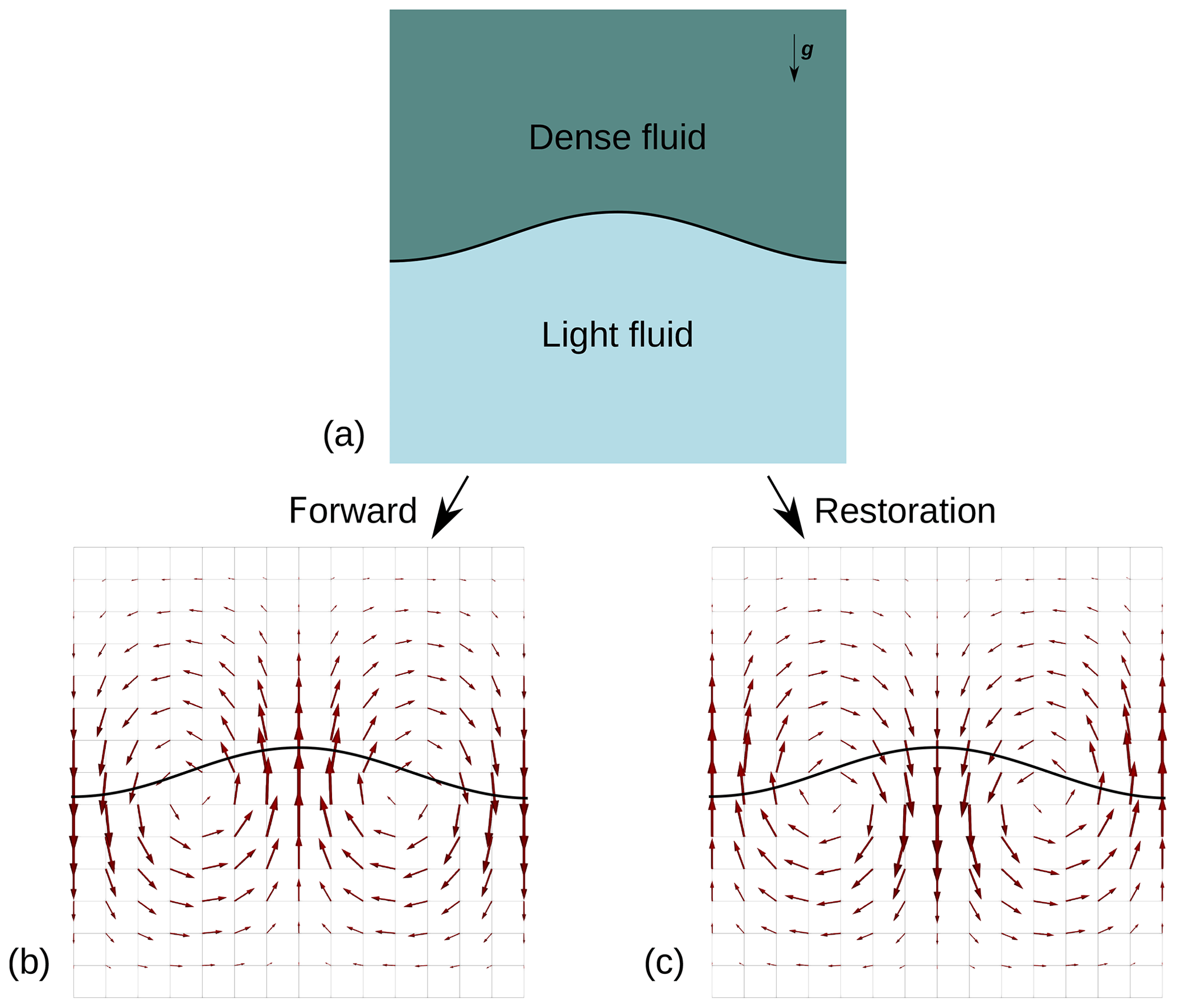
Figure 1 Example of the restoration scheme for a simple setup (a): as the arrows in (b) represent the velocity computed at a specific time step for a forward scheme, the advection of the material model in a restoration scheme is done with the opposite of the computed velocity, shown in (c).

2.2 The FAIStokes code

The restoration scheme presented in the previous section has been implemented in the FAIStokes code described by Schuh-Senlis et al. (2020). It relies on a particle-in-cell (PIC) scheme (e.g., Asgari and Moresi, 2012; Thielmann et al., 2014; Gassmöller et al., 2018, 2019; Trim et al., 2020), where the Stokes equations are solved using the finite-element method (FEM). We review the main characteristics of the code here.

2.2.1 Material discretization

During mechanical simulations, the material properties inside the model are tracked using particles; each of these particles discretizes the small part of the model around it and its properties. At each time step, the material properties of the particles are interpolated from the particle swarm to the FEM grid in order to build the stiffness matrix and its preconditioner. They are then used to solve the Stokes equations, for the velocity, on the grid. Following this, the particles are advected using the solution on the grid.

2.2.2 Viscosity model

During the experiments, we assume the materials to be linear viscous fluids with constant viscosity. While the viscosity of materials is known to vary with the temperature, we do not solve the heat transport equation here. Indeed, in sedimentary basins the temperature is mostly studied for the maturation of source rocks but is not assumed to have sufficient variations to impact the viscosities on our scale. Additionally, the analog laboratory experiment considered in this study (Sect. 3) was performed at room temperature.

2.2.3 Finite-element discretization

In FAIStokes, the Stokes equations are solved on a 2D grid using the FEM algorithms of the deal.II library (Bangerth et al., 2007; Arndt et al., 2019, 2020). Quadrilateral Taylor–Hood Q₂×Q₁ elements, satisfying the Ladyzhenskaya–Babuška–Brezzi (LBB) condition for stability (Donea et al., 2004), are used.

2.2.4 Grid and solvers

The grid and solvers come from the deal.II code. On the right-hand side of Eq. (6), the norm of the gravity vector g of is always 9.81 m s⁻² in our simulations, and its direction can be modified to introduce a tilt in the model. The matrix system is solved using an iterative FGMRES (Flexible Generalized Minimum Residual) solver preconditioned by a block matrix involving the Schur complement (Kronbichler et al., 2012). The grid is adaptively refined and coarsened using deal.II's features based on the position of the faults and the viscosity variability in the elements. An arbitrary Lagrangian–Eulerian (ALE) scheme is also applied on the grid, as explained in the next paragraphs.

2.2.5 Velocity interpolation

Once the Stokes equations are solved in the domain, the velocity is interpolated on the particle swarm using a Q₂ interpolation scheme. Depending on whether the simulation is forward or backward, the displacement of each particle is computed using either Eq. (7) or Eq. (8). The value of the time step Δt is determined from the CFL condition. Finally, the advection is done with a second-order Runge–Kutta scheme in space.

2.2.6 Top surface displacement

During the simulations, the top surface of the model coincides with the top of the computation grid, meaning there is no volume between them. The boundary conditions on this interface are then applied directly to the nodes at the top of the grid. The top surface and model interfaces are tracked by sets of passive tracers in the simulations with an initial horizontal spacing 10 times lower than the material particle spacing. They are advected at each time step the same way as the particle swarm that represents the model. After its displacement or during the setup of the grid, the point swarm discretizing the top surface is used as a reference to vertically move the nodes of the grid at the top of the model so that they match the top surface. This vertical displacement is then propagated to the rest of the grid. The free-surface stabilization algorithm proposed by Kaus et al. (2010) is used in all the simulations which consider the top surface to be a free surface.

3 Presentation of the analog model

3.1 Analog experiment description

The analog model used in this study comes from the deformation of a structural sandbox experiment made by IFPEN (https://www.ifpenergiesnouvelles.fr, last access: 1 August 2024) and C&C Reservoirs (https://www.ccreservoirs.com, last access: 1 August 2024), DAKS^™ (Digital Analog Knowledge System). This experiment aimed to reproduce gravity-driven extensional passive margin structures overlaying a salt layer. The experiment setup is shown in Fig. 2 and presented hereafter.

Figure 2 Setup of the creation of the laboratory analog model from IFPEN and C&C Reservoirs.

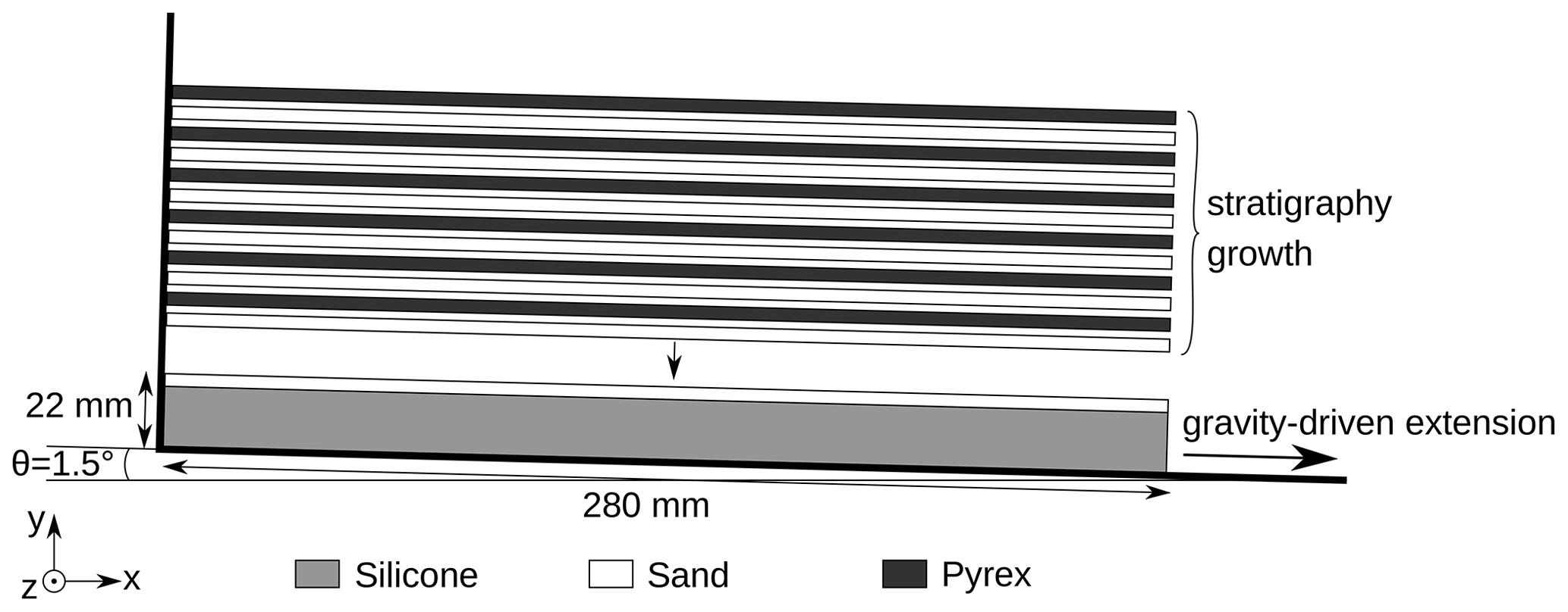
Table 1 Physical properties of the silicone, sand, and pyrex layers for the analog experiment. From IFP and C&C Reservoirs (2006).

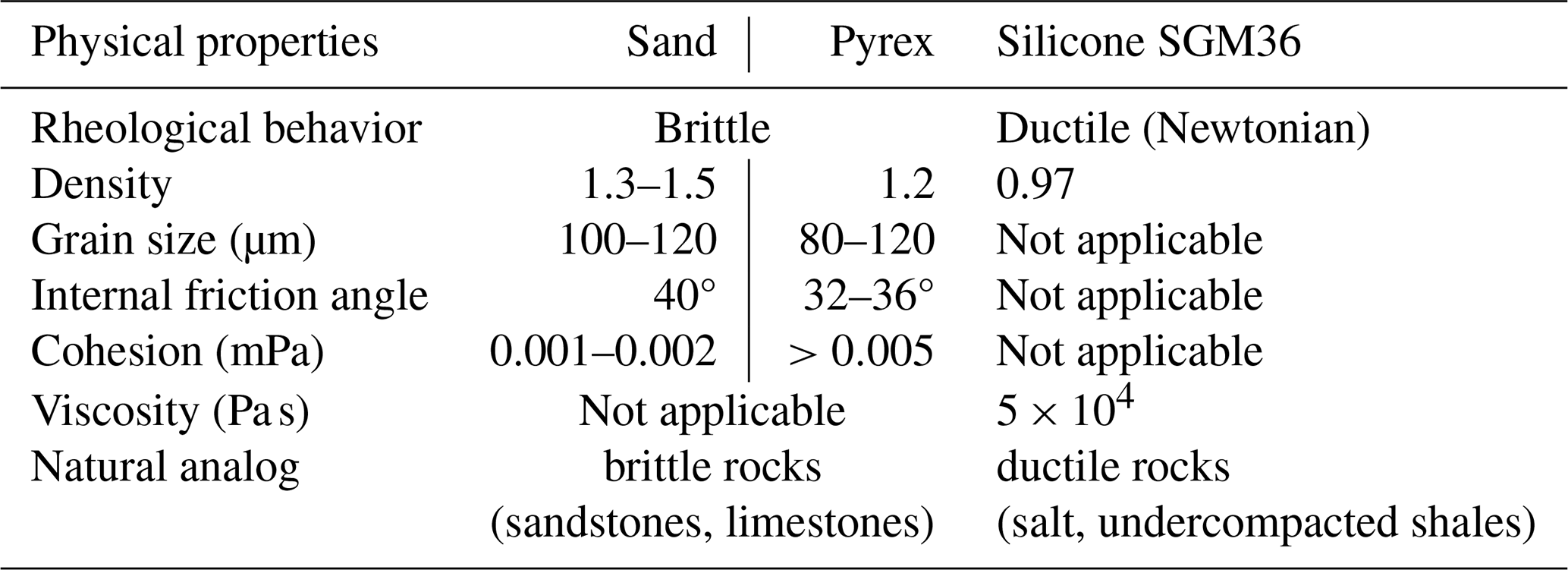
Table 2 Duration of the restoration simulation and topography height after deposition of each layer of the analog model. The indices of the layers are shown in Fig. 4.

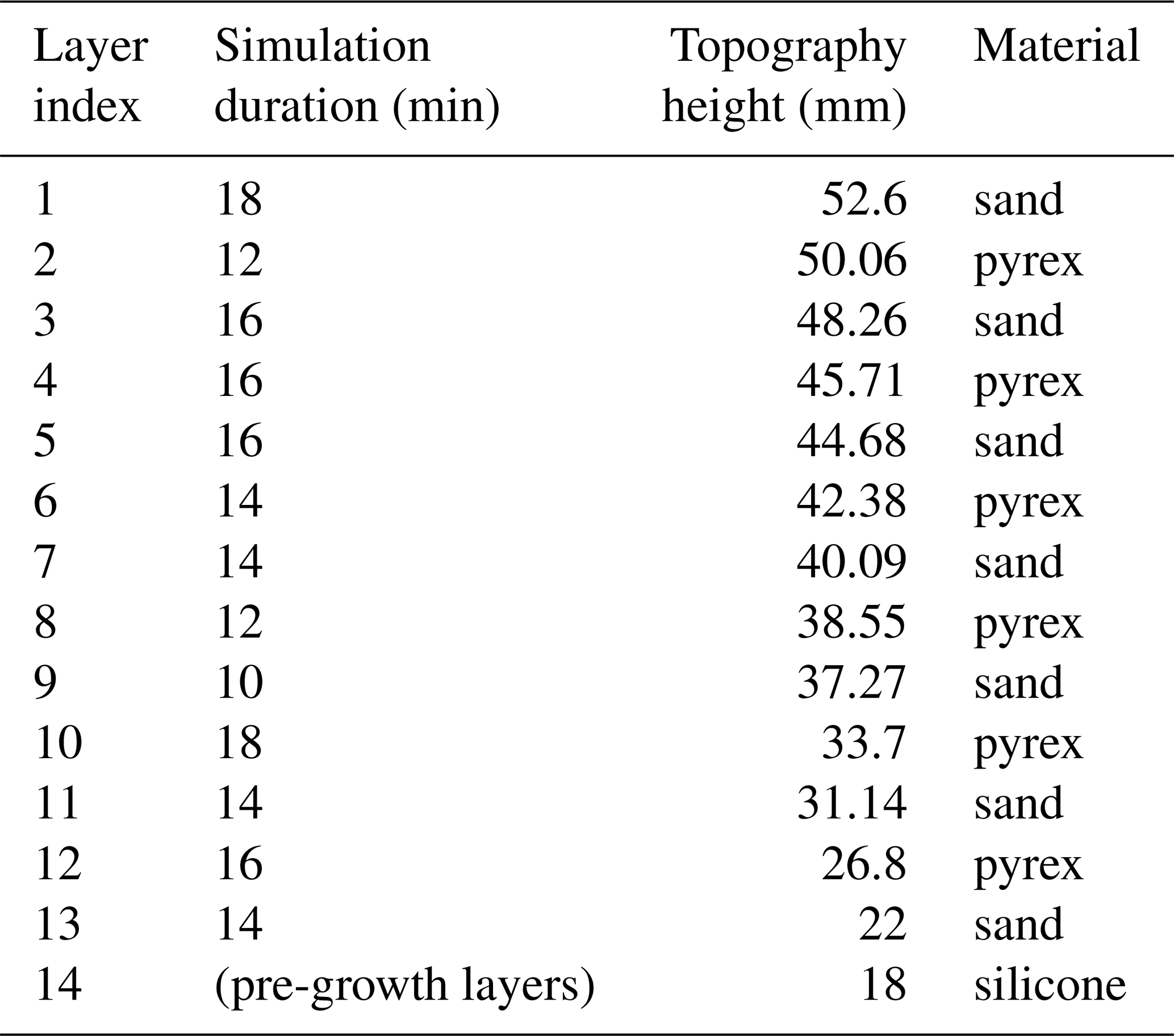
Two initial layers were deposited in the model box, forming the pre-growth strata: a layer of 18 mm of silicone SMG 36 and a layer of 4 mm of sand. On the right-hand side, no boundary was set, while walls were present on the other three sides to prevent the material from moving other than vertically on these interfaces. The model box was then inclined with a 1.5° angle to simulate a basinward tilt, inducing natural gravity-driven extension towards the right-hand side. The experiment lasted for 256 min, during which 12 new layers of alternating pyrex and sand were deposited to simulate stratigraphic growth. This deposition was made in stages at specific time intervals of between 10 and 18 min, as shown in Table 2. These new layers flattened the topography by filling the depressions. The basal silicone material, with a viscous fluid behavior, aims at representing a basal salt layer. The sand and pyrex layers represent clastic sedimentary deposits. The properties of the silicone, sand, and pyrex layers are shown in Table 1.

3.2 Analysis of the experiment using X-ray tomography

The model resulting from the experiment was analyzed using X-ray computed tomography (CT). This method allows the computation of cross-sections without physically cutting the model. As CT is non-destructive, it does not need the consolidation of the model beforehand and avoids the deformation that could occur during the cutting. CT is also fast enough to be used to track the evolution of the experiment. The differentiation of the layers in the cross-sections is done thanks to the difference of density and X-ray attenuation. X-ray tomography images were taken every 2 min, and their resolution is 0.62 mm per pixel. As X-ray tomography is sensitive to density, layer interfaces can be hard to pinpoint where the density contrast is weak. No images were taken during the deposition of sand and pyrex layers, so there are also small time gaps at these moments. These images, however, make it possible to determine both the times between each layer deposition in the forward (laboratory) experiment and the height of the topography after the deposition of each layer (Table 2). The tomography images only cover the left part of the model, so the material flowing on the right-hand side of the model is not tracked. This also means that the velocity on the right-hand side of the model and the total amount of extension are not known. While these are key parameters in understanding basin-forming dynamics, we will show in Sect. 4 how the study circumvents this limitation.

In the present work, we use a cross-section taken at the end of the experiment (Fig. 3) to create an initial model on which to test our restoration method. While this implies working in 2D and therefore ignoring out-of-plane displacements, it significantly reduces the computation time for the restoration process so that more tests on the impact of the different restoration settings can be performed.

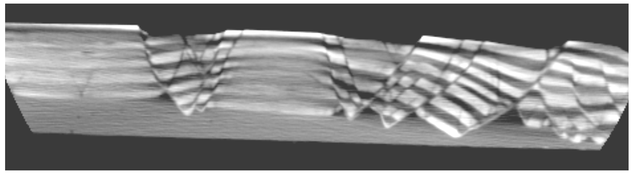
Figure 3 Final cross-section of the analog experiment. The image was obtained using X-ray tomography, with a resolution of 0.62 mm per pixel. As the range of the imaging is limited, the borders of the experiment are not present on the image. CT image from IFP and C&C Reservoirs (2006).

3.3 Creation of the numerical model

To digitize the cross-section in Fig. 3, we first rotate it left by 1.5° to horizontalize the model base and cut it to a rectangular shape. This eases the digitization process and allows for the easier construction of the computation grid around the model. A graphical user interface developed for FAIStokes is then used to digitize the interfaces and the faults in the cross-section. Finally, a particle swarm is created, and the fault and interface lines are used to define the layers and determine the material properties of the particles. The particle swarm contains 667 087 particles at the beginning of the restoration, with a distance of 0.14 mm between each particle. This ensures a minimum of 20 particles per cell during the simulation (for the most refined parts of the grid), even when the adaptive refinement of the grid changes during the simulations.

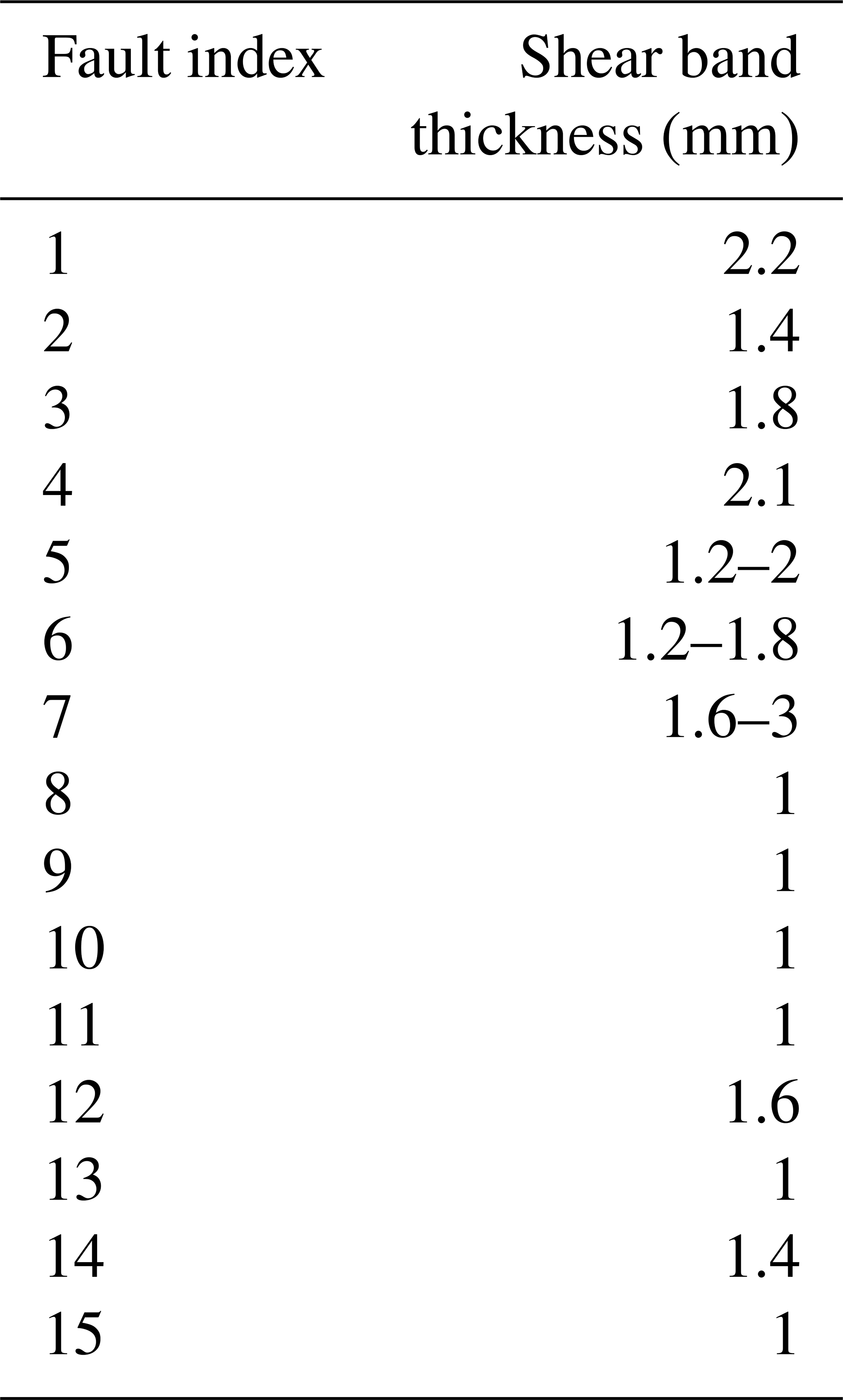
In the faults, the viscosity of the particles is taken to be minimal at the position of the fault line (representing the fault core) and increases with a power law towards the boundary of the shear band, as inspired by Faulkner et al. (2006). The shear band thickness is different for each fault (Table 3). Indeed, a close look at the cross-section in Fig. 3 shows that each fault has a different width of deformation around its core.

Table 3 Shear band thicknesses of the fault in the analog model. The values come from the analysis of the final cross-section (Fig. 3). The index of each fault is given in Fig. 4. The faults with two values have a shear thickness that is reduced at the top of the model because they have a lower deformation range there.

The obtained geometry input to the restoration process can be seen in Fig. 4. In the following numerical experiments, we assume that the model behavior can be approximated using creeping flow as well as geological models, not only in the silicone layer which is chosen to behave so, but also in the brittle and ductile sand and pyrex layers. As there is no inertial part in the deformation of the materials during the experiment, the Stokes approximation can be used. In this type of model, the compaction and decompaction of materials can be important, so we choose to focus on the first restoration step to avoid taking it into account. In the numerical experiments that follow, we make the choice of working at the laboratory scale (width of 280 mm and duration of 256 min), and we use the known silicone viscosity to reduce the number of parameters to test.

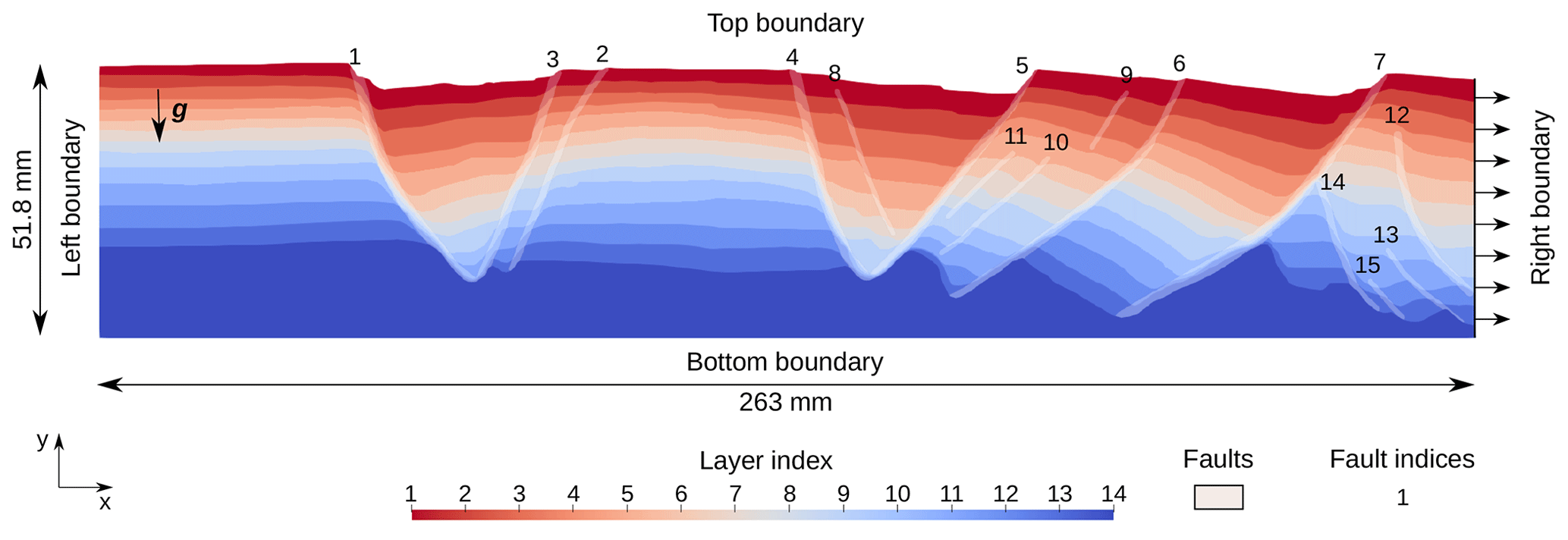
Figure 4 Setup of the analog model to input in FAIStokes for the restoration simulations. The model boundary conditions are not specified here, as their choice and impact on the simulations are discussed in the next section. During the simulations, the tilt of the model is introduced by rotating the gravity vector, as explained in Sect. 2.2.4.

4 Boundary conditions for restoration

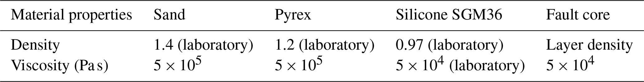
In geomechanical restoration, specific boundary conditions have been used, such as flattening the top surface and applying specific deformation to remove fault throw (by tying the curves representing the footwall and hanging-wall cutoff of horizon surfaces at faults, for example) (Muron, 2005; Chauvin, 2017). Because viscous behavior cannot be handled by elastic material, interfaces between brittle sediments and basal salt layers have usually been considered free surfaces (e.g., Stockmeyer and Guzofski, 2014). Here, we start with simple boundary conditions and show their impact on the deformation inside the model. We then show how more physical assumptions can be used to remove the kinematic part of these boundary conditions. No boundary conditions are applied to the faults, and their deformation depends entirely on the viscosity difference between them and the rest of the model, as specified in Sect. 3.3. In the experiments described in this section, the material properties shown in Table 4 are used. The density of the layers comes from the data (Table 1), and the density of the particles inside the faults is assumed to be the same as in the rest of the layer they belong to. The viscosity of the silicone is known, and we set the viscosity of the sand and pyrex to be 10 times higher. The viscosity at the fault core is set to be the same as inside the silicone. The uncertainty of the viscosity of the sand, pyrex, and fault cores will be addressed in Sect. 5. In all the following experiments, the left boundary condition is set to free slip and the bottom boundary condition is set to no slip.

Table 4 Material properties of the silicone, sand, and pyrex layers in the restoration simulations of Sect. 4. The density of the particles inside the faults is the same as the density of the layer to which they belong. The values that come from the laboratory experiment are indicated.

4.1 Restoration using kinematic boundary conditions

The first boundary conditions we test are kinematic: in the numerical experiment, the motion inside the model is driven by both gravity and the velocity applied at the boundaries. For each layer, the top surface is flattened using a Dirichlet condition: the vertical component of the velocity on the top nodes of the grid at time t is set to

$$\begin{array}{}\text{(9)}& v_y(n,t)=-{\displaystyle \frac{Y_{\text{final}}-y(n,t)}{T_{\text{simulation}}-t}},\end{array}$$

with n the index of the node, y(n,t) its altitude, T_simulation the duration of the restoration for the current top layer, and Y_final the height of the topography at the end of the restoration of the layer (determined from the tomography images and shown in Table 2). The velocity computed in Eq. (9) is in the forward sense, as it is then applied with a backward advection scheme (as in Fig. 1). Following Chauvin et al. (2018), the right boundary is set to a fixed flow. As we consider incompressible flow, the kinematic conditions must ensure the conservation of model volume during the simulation. This means that the volume change due to the topography evolution ΔV_top must be compensated for by the volume entering at the right boundary ΔV_right:

$$\begin{array}{}\text{(10)}& \mathrm{\Delta }{V}_{\text{top}}=\mathrm{\Delta }{V}_{\text{right}}.\end{array}$$

Using the CFL condition (see Sect. 2.1.2), the time step should be computed from the velocity field and change at each time iteration for the computation to be stable. This is an issue here because ΔV_top depends on the time step (computed from the velocity field), and the horizontal velocity at the right boundary determined from ΔV_right is necessary for the computation of the velocity field. To get rid of this dependency, we impose a fixed time step Δt such that the volume change is constant:

$$\begin{array}{}\text{(11)}& \mathrm{\Delta }{V}_{\text{top}}\simeq {\displaystyle \frac{V_f-V_i}{T_{\text{simulation}}}}\mathrm{\Delta }t=\text{constant}.\end{array}$$

The horizontal flow at the right boundary is then applied as

$$\begin{array}{}\text{(12)}& v_x\left(t\right)={\displaystyle \frac{\mathrm{\Delta }{V}_{\text{right}}}{Y\left(t\right)\mathrm{\Delta }t}}={\displaystyle \frac{V_f-V_i}{Y\left(t\right)T_{\text{simulation}}}},\end{array}$$

with Y(t) the altitude of the upper right corner of the model. This means that both the time step and the horizontal flow are constant, but this assumption is necessary from a computational point of view.

The result at the end of the restoration of the first layer is shown in Fig. 5. As imposed by the boundary conditions, the topography at the end of the restoration is flat, and the fault throw is reduced for all the faults. An issue, however, with the use of complete kinematic boundary conditions is the resulting over-parameterization of the system, making it prone to over-steps in the velocity if the volume flow is not perfectly balanced. The fixed time step can, for example, result in particles moving out of the model boundary in the advection step because the CFL condition is not met.

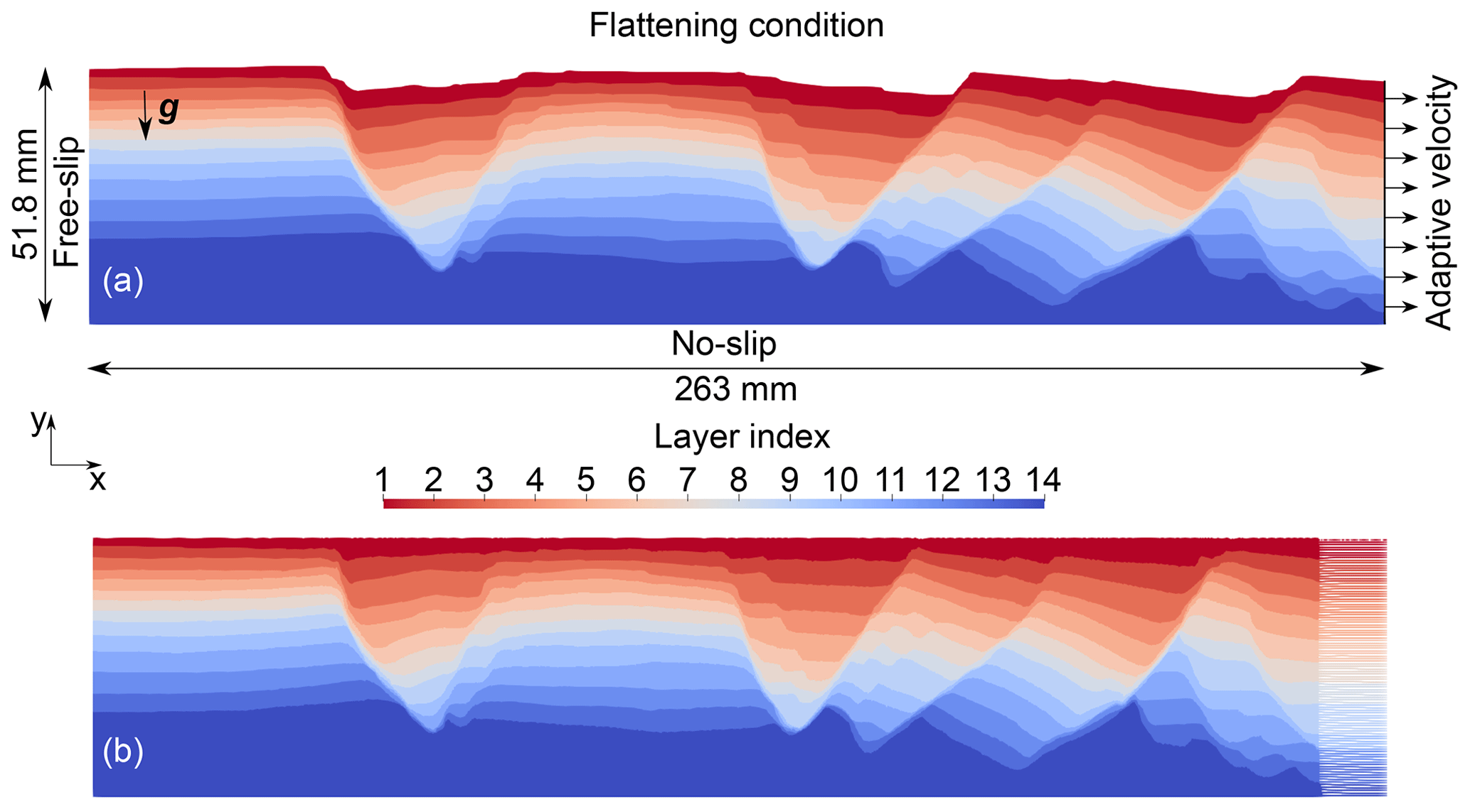
Figure 5 Result of the restoration of the first layer of the analog model. In this case, the left boundary has a free-slip condition, the bottom boundary is set to a no-slip condition, the top is flattened to the topography height at layer deposition, and the right boundary has a velocity condition which adapts to the flattening condition based on Eq. (12). Panel (a) shows the setup at the beginning, and panel (b) shows the state of the model at the end of the restoration.

Figure 6 Comparison between the cross-section image taken by X-ray tomography after the deposition of the last layer (shown in the background) and the restored interfaces at that time (shown as superimposed black lines). The restoration here is performed using the kinematic conditions defined in Sect. 4.1.

To assess the restoration of the layers below the surface, the tomography image taken after the deposition of the last layer is compared to the position of the restored interfaces at this time (Fig. 6). The tomography image is digitized, allowing the computation of the vertical distance d_reference(x) between the restored interface and the actual state of the interface (serving as the reference) at that time, with x the position along the horizontal axis. This distance gives a measure of the error in the restoration of each interface. It is shown in Fig. 7, along with the integral of this distance on the horizontal axis, shown in Table 6.

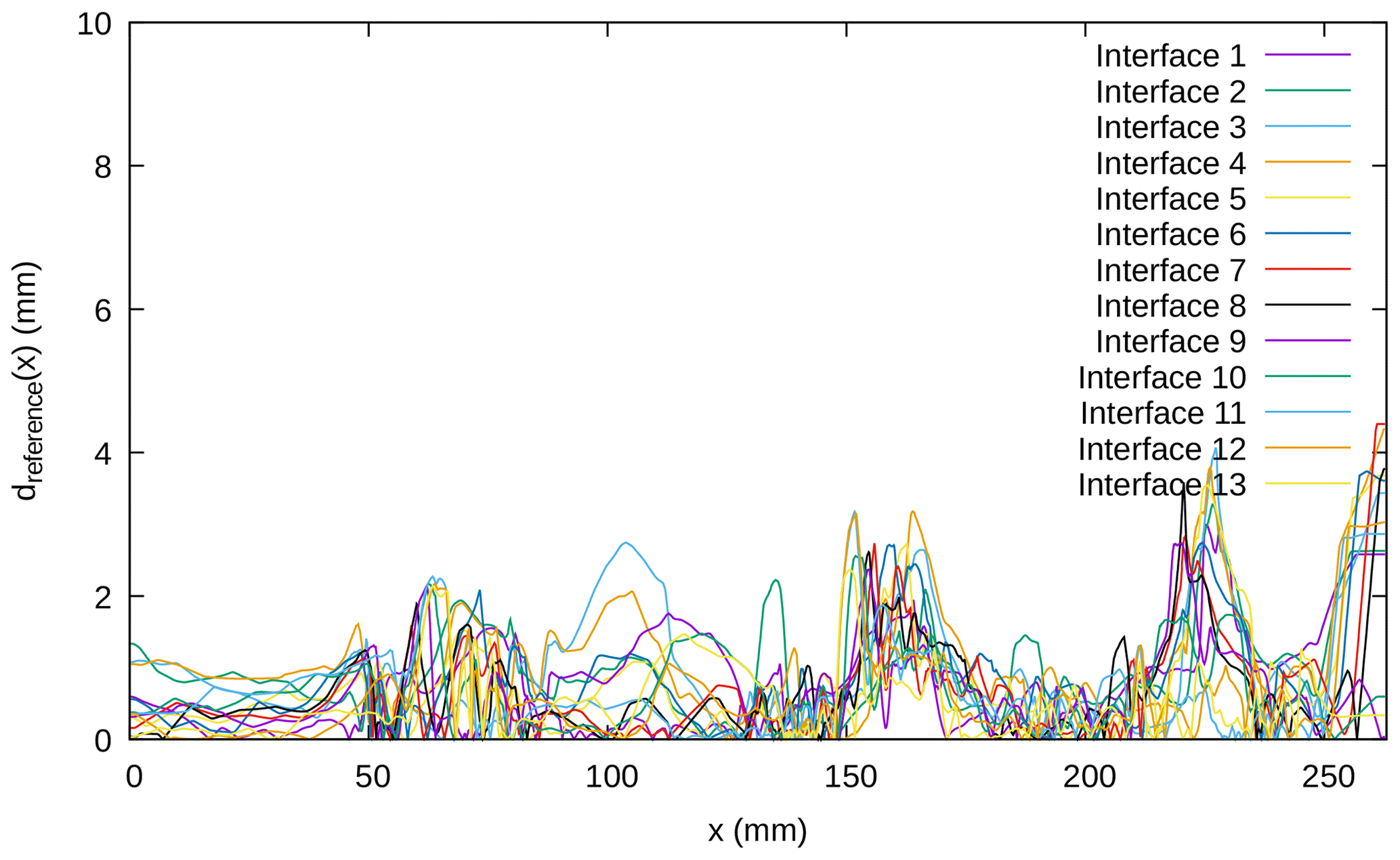
Figure 7 Distance (in absolute value), for each interface between two layers of the model, between the restored interface at the end of the restoration of the first layer and its actual state from the digitization of the corresponding cross-section. The restoration here is performed using the kinematic conditions defined in Sect. 4.1. The interface index corresponds to the index of the layer directly above, starting with interface 1 being the uppermost sand–pyrex interface (see Fig. 4). The digitization of the cross-section has an accuracy of around 1 mm.

Using these results, we see that the error is overall less than 4 mm. The largest errors appear at the right boundary, where the new material entering during the restoration is not known, introducing a high uncertainty to the resulting interfaces. On the one hand, this can be considered acceptable considering the size of the model (52 mm×263 mm) and the accuracy of the cross-section digitization (around 1 mm). On the other hand, it shows that focusing on the restoration of the first layer is already enough to compare the expectations with the restoration results and see errors.

4.2 Choosing more natural boundary conditions

This section aims at trying to remove the kinematic condition to get more natural right and top boundary conditions. Indeed, in the previous subsection, the top surface was set to flattening, which induces external forces applied to the free surface. Moreover, the right lateral boundary was considered to have a constant flow, determined from the top of the tomography images because it was not known inside the model. However, the lateral flow may vary vertically along the boundary.

4.2.1 Relaxing the right boundary condition

First, we focus on the right boundary condition, leaving the top boundary condition with the top surface flattening described in the previous section. To remove the over-parameterization of the model, we want to replace the Dirichlet condition imposing velocity by a force condition. Indeed, during the laboratory experiment, the right-hand side is open, and the model extends freely by flowing with the action of gravity, so the extension front goes further all through the experiment. The scope of the numerical simulations, however, has a fixed extension in time as it focuses on the part where the tomography images were taken. Following Gunzburger and Cornet (2007), we assume that the effective condition applied to the right boundary of the numerical model stems from the weight of the overlying material, part of which is transferred horizontally under a static equilibrium assumption. The weight of the materials on the right side of the model can then be accounted for by introducing a traction based on the pressure on the right boundary. Here, the traction we use is based on the lithostatic pressure p(x,y) inside the model:

$$\begin{array}{}\text{(13)}& p(x,y)=p_{\mathrm{0}}+\underset{y}{\overset{y_{\text{max}}\left(x\right)}{\int }}\mathit{\rho }(x,y)\Vert \mathit{g}\Vert y\mathrm{d}y,\end{array}$$

with p₀ the pressure at the top surface of the model (neglected hereafter). In the case of the analog model, we consider a constant gravity vector g and the density to be constant in each layer, which makes the lithostatic pressure piecewise linear (Fig. 8). The Neumann traction condition applied to the right boundary is then defined as

$$\begin{array}{}\text{(14)}& {\mathit{h}}_N\left(y\right)=-{\displaystyle \frac{\mathit{\nu }}{\mathrm{1}-\mathit{\nu }}}p(x_{\text{max}},y)\mathit{n},\end{array}$$

where the Poisson coefficient is taken as ν_overburden=0.29 in the sand and pyrex layers and ν_silicone=0.33 in the incompressible silicone layer, and n is the outward unit normal vector of the right border. This approximation of the traction and Poisson coefficient values comes from both the literature (e.g., Gunzburger and Cornet, 2007) and tests on various tractions applied at this boundary to find an adequate one.

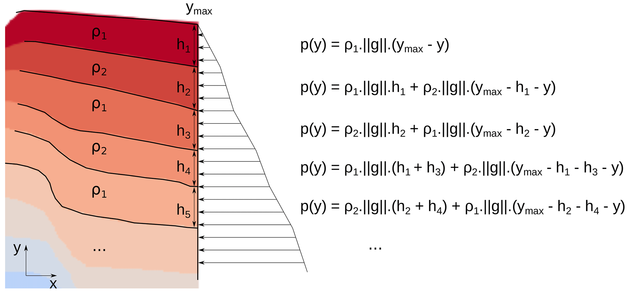
Figure 8 Computation of the lithostatic pressure at the right boundary of the analog model. A cos (θ) factor is then added to the value to take into account the impact of the model tilt on the boundary.

Figure 9 shows the distance between the restored interface at the end of the restoration of the first layer and the actual state of the interfaces at that time along the horizontal axis. The integral of this distance along the horizontal axis is also computed and shown in Table 6.

Figure 9 Same as Fig. 7 with the Neumann condition defined in Eq. (14) on the right boundary.

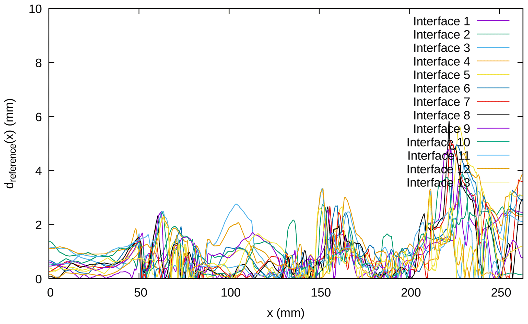
While imputing this new condition on the right boundary removes the kinematic condition and gives it more physical sense, it also increases the freedom of the model and its sensitivity to the material properties. The slight increase in the error in the restoration of the interfaces, compared to the fully kinematic boundary conditions, could then come from inaccurate material properties inside the model. This hypothesis is also supported by the following results.

4.2.2 Relaxing the free-surface condition

In the simulations of the two previous sections, the goal was to test if the model could be restored with creeping flow simulations and a classical topography flattening boundary condition, as well as to estimate the impact of the lateral boundary conditions. While it makes the top surface go back to the state where it was at deposition time, its physical behavior is highly questionable (Lovely et al., 2012). Indeed, as the topography of the model is in contact with air during the analog experiment, a free-surface condition seems more natural. Moreover, flattening means imposing a Dirichlet condition, but the velocity of the topography through time is not known, so an assumption has to be made (we assumed a constant velocity here). Enforcing a velocity condition also makes it uncertain whether the other model parameters are relevant or if they just scale well with the imposed deformation. Here, we test the impact of having a free-surface condition on the top boundary. For this, two restoration configurations were used (the left and bottom boundary conditions being the same as in the previous sections): one with the Dirichlet condition shown in Sect. 4.1 and one with the Neumann condition of Sect. 4.2.1. In these simulations, only gravity and the right boundary condition drive the deformation. Figure 10 shows the top surface of the model after around 15 min of restoration in these two configurations. We can see that imposing the traction (Eq. 14) on the right boundary condition is necessary to balance the model properly or the topography becomes steeper instead of becoming flat during the restoration. When the condition on the right boundary is set to a traction based on the lithostatic pressure, the fault throws of all the faults are reduced during the simulation, and the topography comes closer to being flat. While this balance is encouraging, the model is far from being restored properly, as the model deformation is not consistent with the analog experiment, where the velocity is lower. Too much material is added during the restoration, and the restored horizon is almost universally above the horizontal datum. This shows that removing the kinematic boundary conditions alone is not enough to properly restore a model. The following section will discuss the impact of the material properties and how they can be improved to obtain better restoration results while keeping boundary conditions which do not enforce velocity.

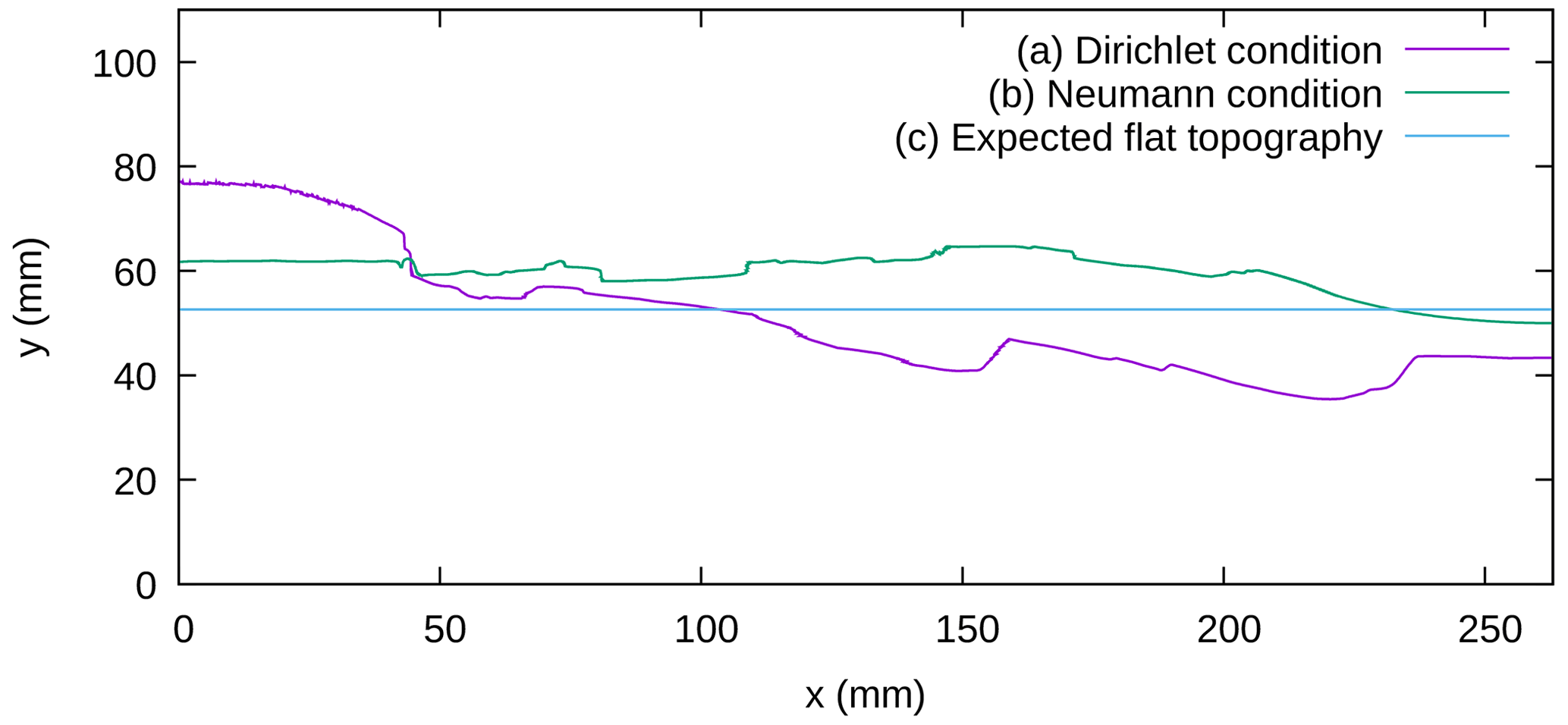
Figure 10 Impact of the boundary conditions on the top surface topography after around 15 min of restoration. The bottom and left boundaries have a free-slip condition and the top is a free surface. The right boundary condition is either (a) a constant flow based on Eq. (12) or (b) the Neumann condition defined in Eq. (14). The expected flat topography is given in (c) as a reference. We see that unphysical Dirichlet condition deforms the topography by bringing up the left part of the model and bringing down the right part of the model. On the contrary, using the traction based on the lithostatic pressure, the whole model is brought up and the fault throws are reduced. We can see, however, that the material properties inside the model do not restore it properly: the top surface ends up being higher than expected.

5 Model material parameter analysis

5.1 Rough estimation of the material properties

In the previous section, the impact of the boundary conditions on the restoration of the analog model was discussed. It showed that removing all kinematic boundary conditions introduced an overestimation of the amount of material entering the model during the restoration. Here, we suggest that finding relevant effective material properties is necessary to improve the restoration process. In this section, the material properties that come from the data are considered to be known and we look for the effective viscosity of the sand and pyrex layers. The boundary conditions are set as shown in Fig. 11. The left boundary is set to a free-slip condition, the bottom boundary is set to a no-slip condition, the right boundary uses the Neumann traction condition defined in Eq. (14), and the top boundary condition is set to a free surface. Doing so, the impact of the choice of material properties on the simulation can be assessed without enforcing the velocity on any boundary.

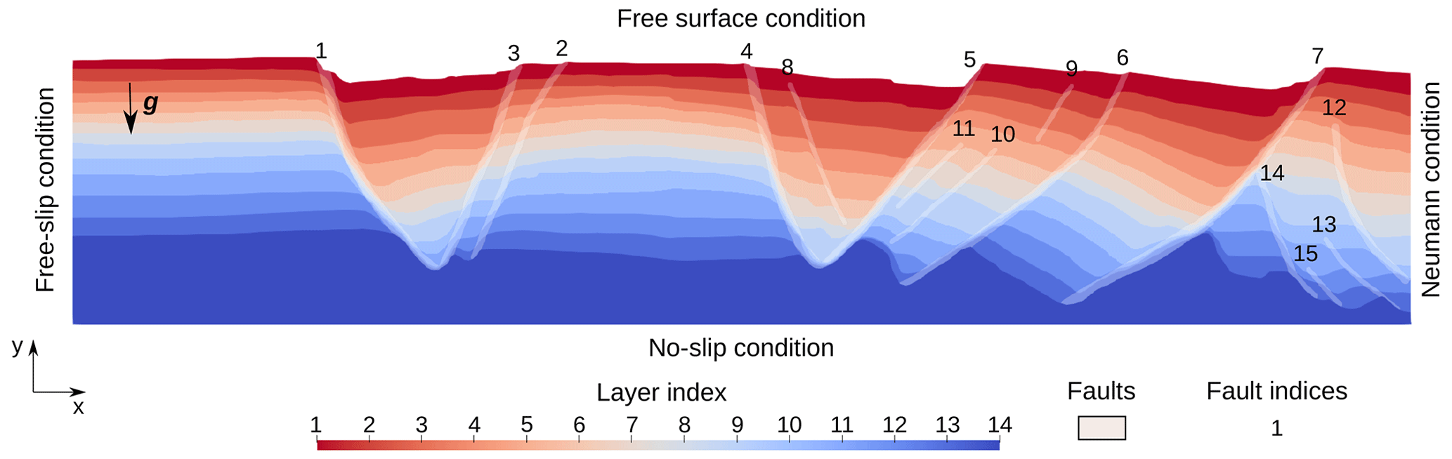
Figure 11 Setup of the analog model to assess the impact of the material properties on the restoration simulations. The right boundary uses the Neumann condition defined in Eq. (14).

As most of the material properties are given as data, only the viscosity of the sand and pyrex layers is left as an unknown. For simplicity, the viscosity is considered to be homogeneous in each layer (outside the faults), with the same value in all the layers no matter whether they are in sand or pyrex. In the faults, the applied viscosity is minimal at the core and increases with a power law up to the contact with the rest of the layers. The range of the viscosity of the sand and pyrex (hereafter called “overburden viscosity”) is chosen as [10⁵:10⁷] Pa s. The viscosity ratio between the silicone and the overburden is then between 2 and 2×10². The range of the fault viscosity is chosen as $[\mathrm{5}\times {\mathrm{10}}^{\mathrm{3}}:{\mathit{\eta }}_{\text{overburden}}/\mathrm{2}]$ Pa s. Eight experiments are conducted, following the parameter choice shown in Fig. 12 for the viscosity of the overburden and faults.

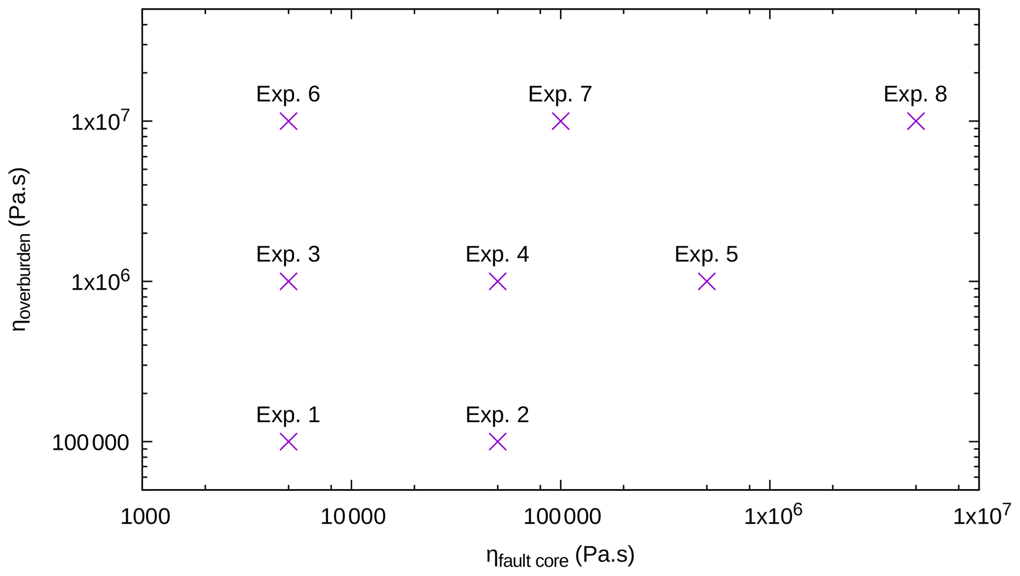
Figure 12 Design of experiments to estimate the effective material properties of the analog model.

To check the quality of the restoration for each experiment, various criteria can be applied. Here, we use the expected topography at the end of the restoration of the first layer as a reference. Indeed, it corresponds to the time in the laboratory experiment where the last layer was deposited (18 min according to Table 2), so for the model to be restored properly the topography should be flat and at a specific altitude at this moment. The implemented criterion then corresponds to the area between the topography of the model at any point x in the restoration and this reference topography. It allows a tracking and comparison of the results throughout the simulation. It is computed as

$$\begin{array}{}\text{(15)}& C_{\text{expected horizontality}}\left(t\right)=\underset{\mathrm{0}}{\overset{x_{\text{max}}}{\int }}\left|y_{\text{top}}(x,t)-y_{\text{expected}}\right|\mathrm{d}x,\end{array}$$

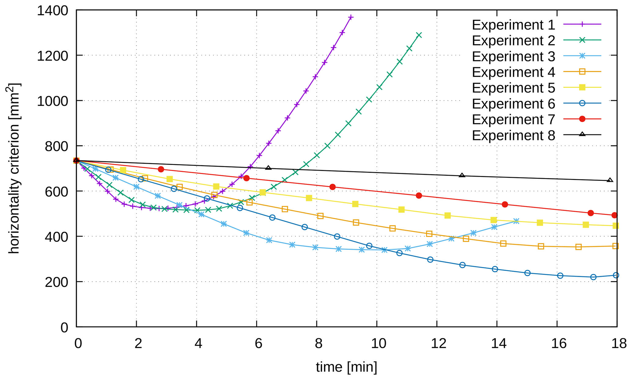
where x_max is the domain length, y_top(x,t) is the altitude of the topography along the x axis at a given time t, and y_expected is the expected altitude of the topography at the end of the restoration of the layer (from Table 2). This criterion is hereafter referred to as the expected horizontality criterion. It has several advantages: first, it is relatively simple to compute and track throughout the restoration simulations. Second, it gives a value of the global difference between the model and the expected restoration result with a flattened top layer. Third, it can be used to compare simulations which evolve at different velocities and to check when they start to evolve in the wrong direction (i.e., creating relief in reverse time).

The values of the expected horizontality criterion through time for the eight experiments are given in Fig. 13. The results are shown for 18 min, which corresponds to the restoration of the first layer (Table 2). In all the experiments, we can see that the model deformation starts by going towards a flat topography at the expected altitude (the expected horizontality criterion decreases towards zero). In experiments 1 to 3, after some time this behavior changes and the model topography evolves away from the expected altitude. In the other experiments, the expected horizontality criterion decreases but does not reach zero before the end of the layer restoration. In experiments 1 to 3, we let the simulations continue after the criterion started to increase for testing purposes. Such an increase could, in practice, be used to detect when a restoration simulation is wrong (because of computational instabilities like those present in Sect. 4.2.2 with a Dirichlet condition on the right boundary, for example) and to stop the simulation.

Figure 13 Values of the expected horizontality criterion (Eq. 15) throughout time for the simulations of the design of experiments (Fig. 12) to find the effective material properties inside the analog model.

While the expected horizontality criterion is good to determine the global distance between the simulations and the expected result, it is not enough to determine the “best” material parameters for the restoration. Figures 14 and 15 show the state of the model for each experiment at the time t_final of their last point in Fig. 13 in order to analyze the impact of each parameter involved in the design of experiments in a more detailed way.

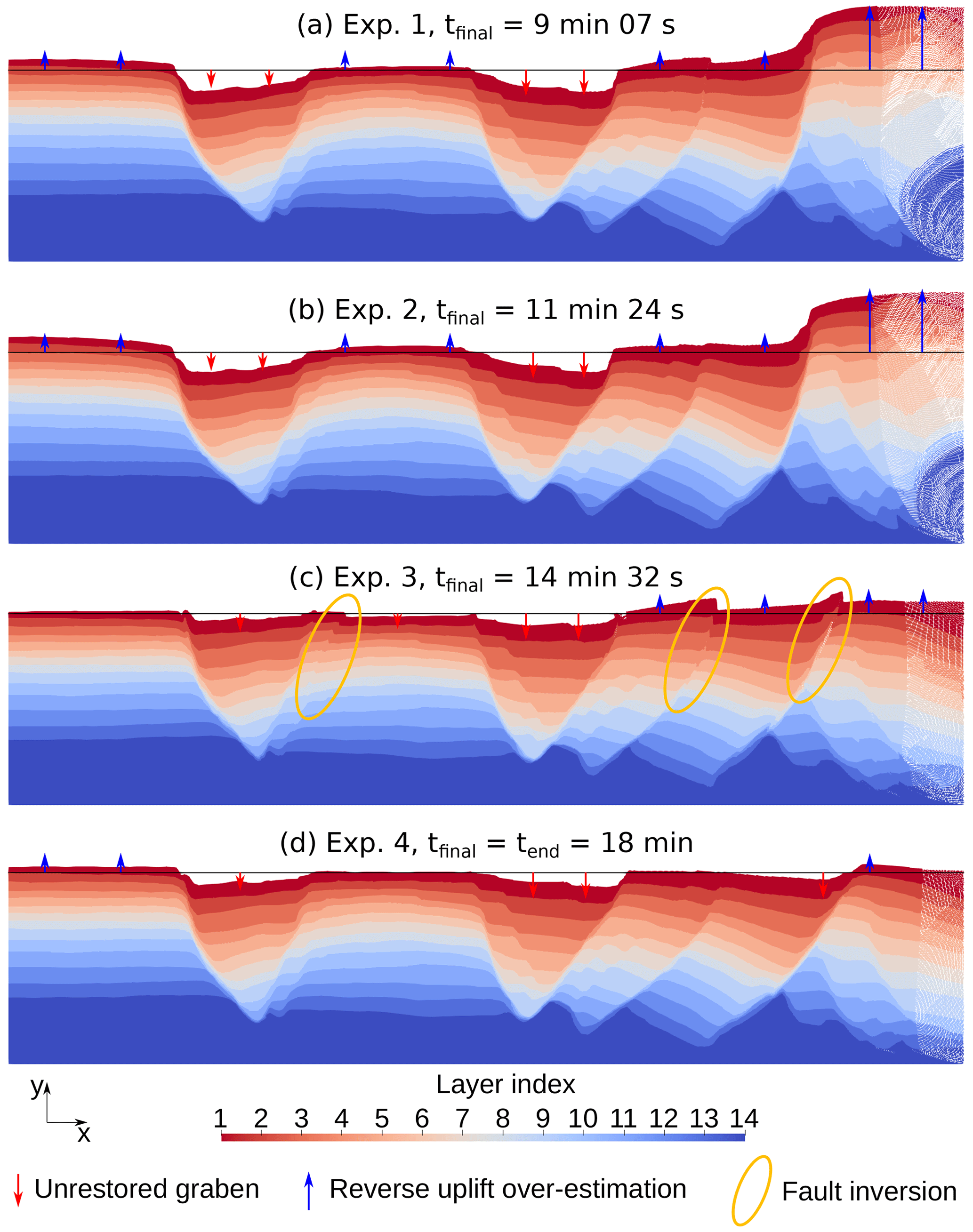
Figure 14 Results of experiments 1 to 4 (Fig. 12) to find the effective material properties inside the analog model. For each experiment, t_final is the restoration time at which the simulation is stopped and for which the model is shown. t_end is the time at the end of the restoration of the first layer. The black line on each result is the expected position of the topography at the end of the restoration of the first layer.

Figure 15 Same as Fig. 14 for experiments 5 to 8.

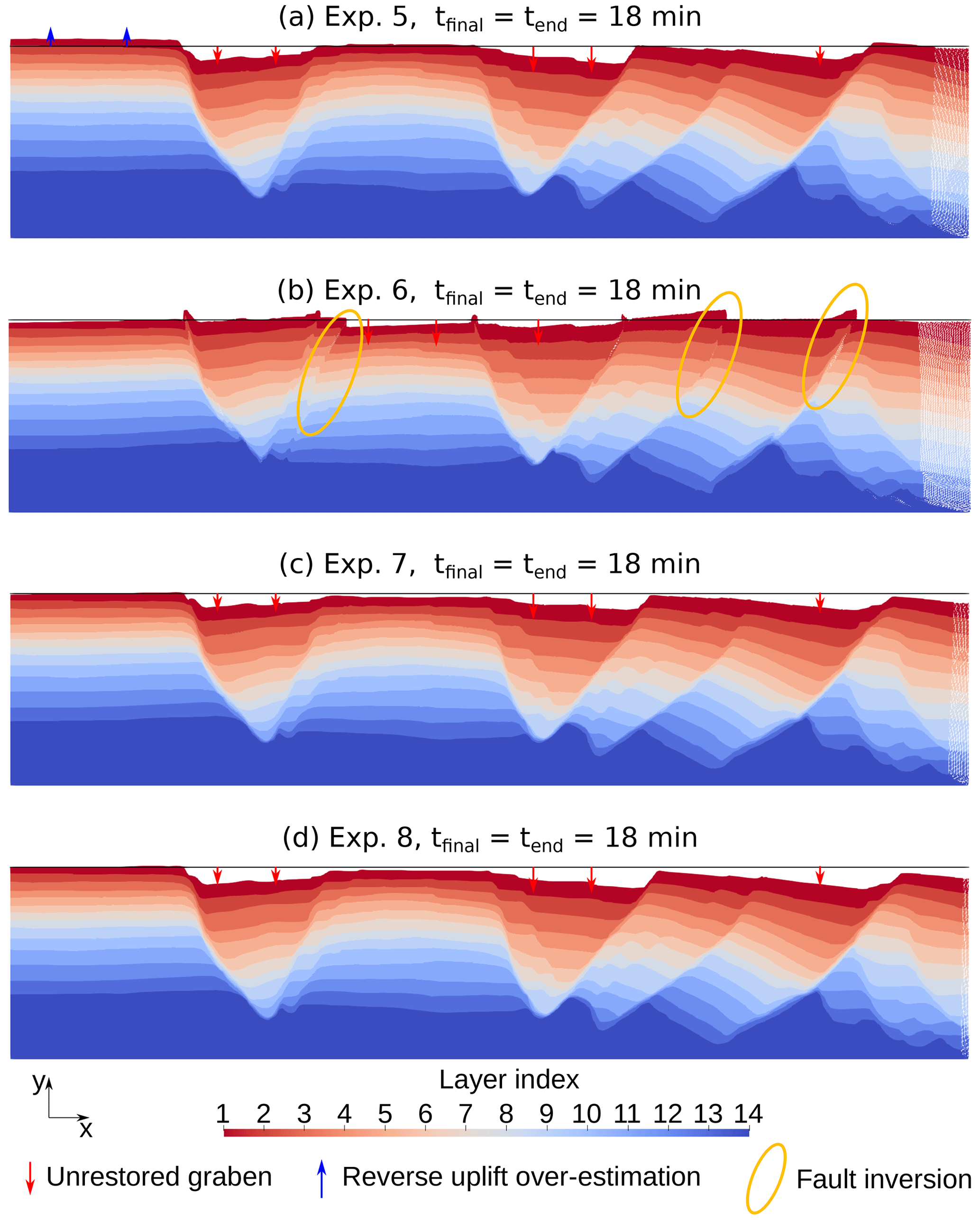
In experiments 1 and 2, the rapid increase in the expected horizontality criterion is explained by the right part of the model going up. The overall restoration also shows that the thicknesses of the overburden layers increase too much, while the fault throws are not reduced much during the simulation. It can be explained by the viscosity of the overburden being too low compared to the viscosity of the faults. In experiment 3, we observe that the fault throws are overall reduced, but some of them get inverted (on faults 2, 6, and 7, with the numbering of Fig. 4), suggesting that the viscosity of these faults is too low. In experiment 4, as in experiments 1 and 2 (but not in the same proportions), the deformation of the left and right parts of the model is a bit strong, while the fault throws are not reduced much, showing that the viscosity of the faults is not low enough, while the viscosity of the overburden is too low. In experiment 6, the fault throws are overall reduced or canceled. Although it shows the smallest value of the expected horizontality criterion (Fig. 13), faults 2, 6, and 7 (with the numbering of Fig. 4) start to invert their throw, like in experiment 3, showing that their viscosity is too low compared to the viscosity of the overburden. In experiments 7 and 8, the overall deformation is too small, showing that the viscosity of both the overburden and faults is too high.

The results of these experiments show that it is possible to narrow down the possible values of the effective parameters in this type of model. It also shows, however, that the viscosity of the materials at play cannot be modeled by a unique value for all the material types. Particularly, imposing the same viscosity on all the faults seems like a wrong assumption. Indeed, fault histories and mechanical properties differ in the experiment as in real geological settings. In the following, we try to improve the simulations by imposing a different viscosity from one fault to the other.

Figure 16 Values of the expected horizontality criterion (Eq. 15) through time for the restoration with a fine tuning of the fault viscosity (yellow curve) compared to some experiments of Sect. 5.1.

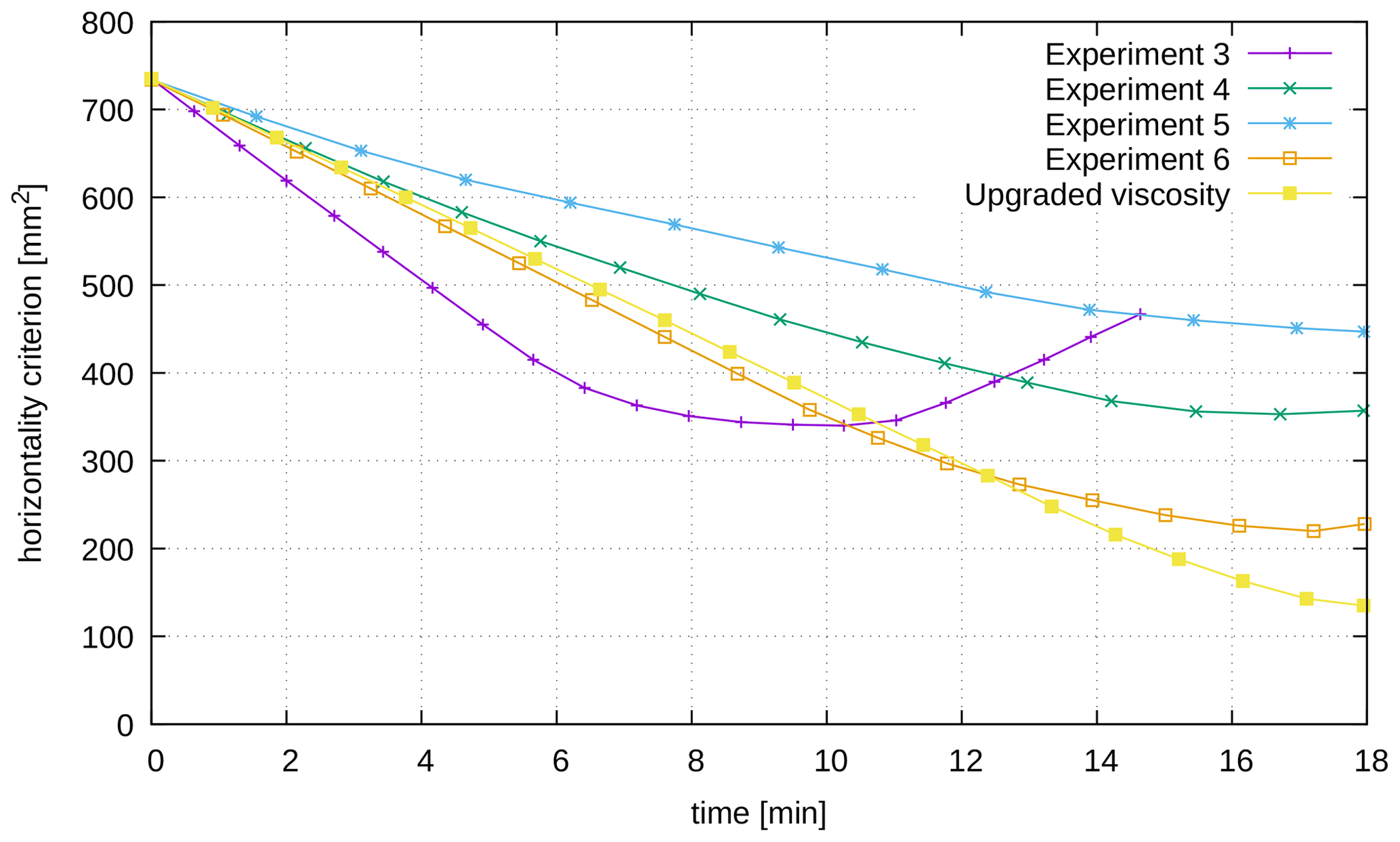
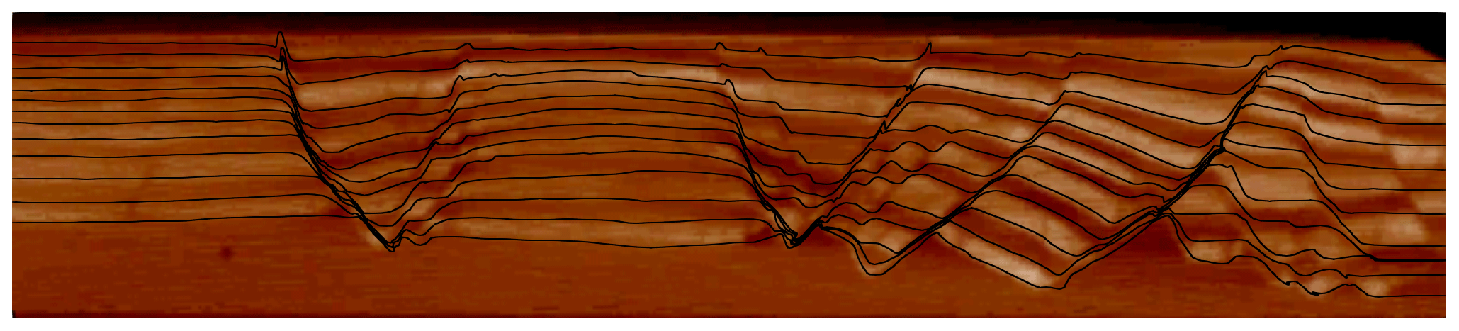
Figure 17 Comparison between the cross-section image taken by X-ray tomography after the deposition of the last layer (shown in the background) and the restored interfaces at that time in the restoration process (shown as superimposed black lines). The restoration here is done using the boundary conditions and model parameters of Sect. 5.2.

5.2 Fine tuning of the material parameters

Given the previous results, the viscosity of the faults looks like an important parameter to improve restoration. More specifically, the fault inversion appearing only on some faults in experiments 3 and 6 calls for a specific treatment of each fault. In the following, we carry out tests to estimate the viscosity within each fault. The material properties that were considered to be known in the previous section do not change (see laboratory values in Table 4). Based on the previous results, the viscosity in the overburden layers is set to 8×10⁶ Pa s, and the default viscosity at the core of the faults is set to 5×10³ Pa s (close to their value in experiment 6). Starting from this default value, various tests are performed by multiplying it by different factors (from 0.75 to 3) in each fault. The factors which give the best restoration results are shown in Table 5. For this restoration, the values of the expected horizontality criterion as a function of time are compared to previous results (Fig. 16). They show that a fine tuning of fault properties upgrades the global restoration and makes the model closer to being flat at the end of the restoration simulation. In order to look at a more global criterion, Fig. 17 shows the comparison between the tomography image taken after the deposition of the last layer and the position of the restored interfaces at this time. The integral of this distance along the horizontal axis is given in Table 6. Overall, the analysis of the restored interfaces yields lower restoration errors than with fully kinematic boundaries. Both the visual (Fig. 17) and quantitative comparisons of the X-ray tomography image and the restored interfaces show that the restoration is better on most of the interfaces. The highest errors come from the faults, where the low viscosity induces a “squeezing” effect on the material inside the shear band during the simulation, resulting in an upward motion at their position, particularly near the top of the model.

Table 5 Factors by which to multiply the default fault core viscosity to obtain the best restoration result in Sect. 5.2. The fault indices are defined in Fig. 4.

Additionally, Fig. 18 shows, for each layer interface, the vertical distance between the restored interface and the actual state of the interface at that time along the horizontal axis.

Figure 18 Same as Fig. 7 with the boundary conditions and model parameters of Sect. 5.2.

Table 6 Integral, for each interface between two layers of the model, of the distance between the restored interface at the end of the restoration of the first layer and its actual state at this time, digitized from the corresponding cross-section. In the first line, the restoration is done using the kinematic conditions (flattening on top and Dirichlet condition on the right) defined in Sect. 4.1. In the second line, the restoration is done using the conditions defined in Sect. 4.2.1 (flattening on top and the Neumann condition defined in Eq. 14 on the right boundary). In the last line, the restoration is done using a free surface on top and the Neumann condition defined in Eq. (14) on the right boundary. The interface index corresponds to the index of the layer directly above from the indexation of Fig. 4.

These results show that it is possible to obtain slightly better restoration results by removing kinematic boundary conditions and replacing them with more natural conditions. This, however, requires a long analysis of the material parameters to find some that are as close as possible to the effective ones. While this process gives valuable information on the effective viscosity to apply in numerical simulations of viscous-based models, it also shows that restoration with “natural” boundary conditions is not as simple to obtain as one would hope.

6 Discussion

Previous restoration approaches have shown that geomechanical schemes can be used to add physical meaning to the restoration process (e.g., Maerten and Maerten, 2001; Muron, 2005; Moretti et al., 2006; Durand-Riard et al., 2010; Chauvin et al., 2018) and account for specific rheological behavior such as that of salt rock (e.g., Kaus and Podladchikov, 2001; Ismail-Zadeh et al., 2001, 2004). Recently, Schuh-Senlis et al. (2020) showed that creeping flow restoration could be applied to synthetic basin models which include salt, faults, and a free-surface condition at the top. To go further, we applied the restoration process of Schuh-Senlis et al. (2020) to an analog experiment model here. This allowed us to test the results of the creeping flow restoration method on a model obtained by the deformation of an actual material, specifically one (sand and pyrex) that is not ideally represented as a Newtonian fluid. The deformation history images on a cross-section were used to quantify the accuracy of the restoration results, and some reference rheological values of the laboratory analog experiment (e.g., silicon viscosity) were introduced in the numerical model to make our test simpler.

While neglecting the inertial part of the Navier–Stokes equations in simulations at the scale of the analog model is questionable, this hypothesis is supported by three points. First, the displacement during the experiment is sufficiently slow to neglect any inertial effects. Second, the restoration results back up this assertion. Third, this is a limit case to test the validity of the method on an analog experiment, and the application on the corresponding geological model would verify the same hypothesis, as stated in Sect. 2.1.1.

The first tests on the analog experiment model showed that the first layer of the model could be restored properly with kinematic boundary conditions such as those used in standard geomechanical restoration. Other boundary conditions were then tested to remove the kinematic part of the conditions, namely a Neumann traction condition on the right boundary, which accounts for the lithostatic pressure, and a free-surface condition on the top surface of the model. While these boundary conditions seem to better reflect the tectonic settings, the erratic results obtained suggested that changing the boundary conditions alone was not enough to restore the model properly. They also suggested that they could be used to detect errors in some model parameters (e.g., the other boundary conditions and the material properties, specifically the effective viscosity). When building on this error detection to find more appropriate material properties, it was shown that the restoration results could even be improved, albeit slightly, despite removing all kinematic conditions.

The case of the left and bottom boundaries has not been discussed much. The tests used a free-slip condition on the left boundary and a no-slip condition on the bottom boundary, but these assumptions are simplifications, and a friction condition on the bottom and a Neumann condition on the left-hand side might be more physical. Several tests showed, however, that the difference between a free-slip and no-slip condition on the two boundaries impacts the simulations only if they are otherwise unbalanced (by a wrong traction on the right boundary, for example).

For the right boundary, our static equilibrium assumption entails that the traction applied depends directly on the Poisson coefficient. In our study, we set this coefficient from reference values for the type of granular material in the model, but its impact may have to be estimated more properly and more precisely. Indeed, additional tests have shown that while the Poisson coefficient value does not impact the general behavior of the model, it can impact the value of the best effective viscosity inside the model. Another possible issue with the traction at the right boundary of the model is the account of the tilt and its implications for the material on the other side of the boundary. Here, we did not consider the impact of the movement of this material, as the Stokes equations ignore the inertia of the material. It poses, however, the following question: does the movement of surrounding materials impact the horizontal pressure applied by them to the boundaries of the model? In this case, the traction would have to be changed accordingly.

The tests done on the boundary conditions of the analog experiment model also showed that when no kinematic condition was applied, the material properties initially assumed do not allow the restoration of the model. To study their impact and to find the best effective properties inside the model, the restoration scheme was applied to eight models with different properties following a design of experiment. As the viscosity of the silicone and the density of all materials were known, the parameters we studied were the viscosity inside the faults and the viscosity in the sand and pyrex layers. The first experiments helped narrow down the range of values for these effective viscosities and showed that a different effective viscosity has to be used for each fault in the model. Various experiments then allowed us to tune the viscosity inside the faults accordingly and decrease the restoration error. This viscosity tuning, however, was done manually and we could not find a relation between the viscosity difference between the faults and their difference in age or shear band thickness. To find how to guide the choice of the fault effective viscosity, more tests using a local criterion on the fault throw for each fault may then be necessary.

The hypothesis of a viscous fault behavior could also be revisited in future studies. The frictional fault surfaces might be considered, but this would compromise the reversibility assumptions used in restoration methods to date. Another option for future investigations could be to consider time-varying viscosity to decrease fault viscosity down to that of the intact rock when the fault displacement reaches zero. Looking into which viscous fault behavior drives fault inversion could also provide new insights on basin inversion. Along the same lines, it could be interesting to study the influence of accumulated strain (by considering the sand and pyrex layers to be visco-elastic materials) or of a variable viscosity in the layers (depending on the type of layer or on the age and altitude, for example).

An issue that remains to be addressed is the fact that a lower viscosity inside the faults can lead to overestimations of the horizontal velocity for the faults. In restoration simulations, this leads to the material inside some of the faults being pushed out by the blocks with higher viscosities on the sides. The application of an anisotropic viscosity may remove this issue but has not been studied yet.

To further assess the use of creeping flow restoration without kinematic conditions, it would also be interesting to apply it to other structural models. The use of other analog experiment setups would allow researchers to check the validity of the conditions that were found in this paper. It would also provide the effective properties in a wider range of model deformation types (other extension profiles, regression, etc.). The comparison of the effective viscosity in different analog models, for example, could provide interesting data when scaling the effective properties to apply the method to models of the subsurface at geological timescales.

While adding more physical conditions to geomechanical restoration is interesting in itself, the goal is also to provide a working method for the restoration of models describing the subsurface in real cases. Several questions would then arise. First, the scope of this study was the restoration of a 2D cross-section. This not only neglects the out-of-plane displacement, but also reduces the scope of the boundary conditions and material properties. It is uncertain, for example, how the viscosity of faults would have to vary laterally in a 3D model to be able to restore them properly. Second, the boundary conditions may be more complicated with the addition of continuous erosion and sedimentation to the topography (compared to punctual sedimentation in the analog experiment). The forces at play several kilometers deep in the underground are also unknown, and the bottom boundary may be more complex than the free-slip and no-slip conditions applied here. For example, specific flow due to uplift or subsidence of the layers below the model may need to be taken into account. The pressure applied to the lateral boundaries may also prove to be more challenging in heterogeneous media with variable density and mechanical properties. Finally, the space of material parameters to be estimated would be much bigger than that of an analog experiment model. To reduce this space, research could be done on a way to scale the effective parameters from those of the analog experiments to real case models with the same deformation mechanisms. Interestingly, to answer these questions, creeping flow restoration could be a useful tool: using the flattening condition as a likelihood metric, the conditions that best balance the models could be determined as the solution to an inverse problem for the restoration results.

7 Conclusions

In this paper, we have shown the results obtained with the creeping flow restoration method for a structural model obtained from a laboratory-scale analog model including multiple faults. Conclusive results can be obtained with classic kinematic boundary conditions. The study then aimed at removing the kinematic part of the boundary conditions to leave more freedom to the model and assess the impact on the restoration results. It showed that when replacing kinematic conditions with force conditions closer to those of the actual tectonic settings, the model could not be properly restored without material parameters as close as possible to the effective ones.

Using these boundary conditions, however, it was possible to assess the impact of changing the material properties inside the model. By going closer to the effective material properties, we were even able to obtain slightly better results than those using kinematic boundary conditions for the restoration. These results both improve the physical meaning of the restoration and provide valuable information on the effective material properties to use in mechanical simulations.

As such, the creeping flow restoration of this analog experiment model shows that this restoration scheme can be applied to relatively complex structural models in 2D, without any kinematic boundary conditions. This, however, implies a complex trial and error process to find the effective material properties, without which the restoration process is not possible. We believe that further investigations and numerical tests are needed for progress to be made on physically based restoration, especially to analyze the trade-offs between geometric uncertainties in the structural model, material behavior law and the associated properties, and boundary conditions.