Revisiting Gassmann-type relationships within Biot poroelastic theory

Gassmann's equations have long served as a cornerstone of geophysics and rock physics, widely regarded as exact within their domain of applicability. However, recent studies have questioned their validity, arguing that Gassmann's derivation involves a logical error and that an additional solid modulus is needed even for monomineralic materials. In this work, we present a general derivation of the extended Biot poroelasticity equations, grounded in conservation laws and classical irreversible thermodynamics (CIT). We show that the formulations of Gassmann (1951), Brown and Korringa (1975), Detournay and Cheng (1993), and Rice and Cleary (1976) emerge as special cases of this unified framework. While previous studies have analyzed the thermodynamic admissibility of standard Biot and Gassmann models, we extend this analysis to the more general theory by explicitly incorporating the off-diagonal terms arising from the second partial derivatives (Hessian) of internal energy. A key finding is that Gassmann's self-similarity condition – that porosity remains unchanged under equal changes in fluid and total pressure – is a sufficient but unnecessary condition for the derivation of Gassmann-type relationship between undrained and drained bulk moduli. It holds if and only if the matrix of the second partial derivatives of internal energy is diagonal. When the off-diagonal terms in this matrix are retained, a generalized form of Gassmann's equations is required, which we derive. To promote transparency and support further research, we provide symbolic Maple routines with thermodynamic consistency checks, ensuring full reproducibility and accessibility.

1 Introduction

Gassmann's equations (Gassmann, 1951), developed several decades ago, are fundamental in geophysics for analyzing the elastic properties of fluid-saturated porous media. These equations provide a means to predict seismic velocities and mechanical behavior in such materials. However, despite their widespread use, recent studies have questioned the logical consistency of Gassmann's derivation, suggesting that it contains a logical error (Thomsen, 2023a, b, 2024, 2025). This has highlighted the need for an extended, transparent, and thermodynamically consistent framework to ensure reliability in geophysical modeling and interpretation.

This paper presents a structured, transparent, and fully reproducible derivation of the extended Biot poroelastic equations, with the formulations of Gassmann (1951), Detournay and Cheng (1993), Brown and Korringa (1975), and Rice and Cleary (1976) emerging as special cases. Our approach is rooted in fundamental conservation laws and classical irreversible thermodynamics (CIT) (Lebon et al., 2008). While earlier works have demonstrated the thermodynamic admissibility of the standard Biot and Gassmann models (Coussy et al., 1998; Yarushina and Podladchikov, 2015), we extend this analysis to a broader class of models by evaluating the full Hessian matrix (i.e., matrix of second partial derivatives) of internal energy.

We respond directly to the critiques presented in Thomsen (2023a, b, 2024, 2025), adopting the CIT formalism as described in Lebon et al. (2008) and extended to poromechanics by Yarushina and Podladchikov (2015). We demonstrate the thermodynamic admissibility of the extended Biot equations by incorporating entropy production constraints and the internal-variable formalism of CIT. Internal consistency is verified through both theoretical analysis and numerical evaluation. In particular, we emphasize the interplay between thermodynamic forces and fluxes, entropy production, and the admissibility of constitutive laws.

The paper is structured as follows: we begin by reviewing the foundational equations of classical irreversible thermodynamics, highlighting the roles of thermodynamic forces and fluxes. We then derive the evolution equations for the extended Biot poroelastic system, followed by formulations of the Detournay–Cheng (DC), Brown–Korringa (GK), and Gassmann models. Afterwards, we revisit Gassmann's assumptions and delineate the specific conditions under which they remain valid. We also directly address the critiques raised in Thomsen (2023a, b, 2024, 2025) regarding the validity of Gassmann's equations.

To ensure full reproducibility, we provide symbolic Maple routines with detailed line-by-line commentary, enabling transparent derivation and verification. This framework also supports future extensions, including multiphase flow and viscous deformation mechanisms. All Maple scripts are available in a symbolic archive via a permanent DOI on Zenodo: https://doi.org/10.5281/zenodo.15777522 (Alkhimenkov and Podladchikov, 2025).

2 Scope of the article

One can distinguish between two related but distinct tasks in the formulation of coupled (poroelastic) theories: (i) identifying the appropriate set of state variables that fully describe the coupled mechanical behavior and (ii) deriving the material parameters that link these variables. Task (i) is particularly challenging and has been addressed by numerous researchers; a comprehensive review is beyond the scope of this article. In this work, we build on those earlier studies and assume from the outset that the correct variables have been identified.

Task (ii), while relatively more straightforward, remains essential: various modifications of poroelastic theory have been proposed, often based on simplifying assumptions that affect how material parameters are defined and interpreted. The main novelty of this article is the consideration of the full Hessian matrix of second derivatives of internal energy, including the off-diagonal terms (which are often neglected in classical formulations), which enables us to derive a generalized set of Gassmann-type relations. Furthermore, we demonstrate that, under appropriate mappings between poroelastic coefficients, several classical poroelastic theories can be viewed as equivalent.

3 Derivation of the extended Biot's poroelastic equations

General pattern of the derivation

To derive the extended Biot poroelastic equations, one typically combines the following components:

• Conservation laws

  • Conservation of linear momentum for the total stress,

  • Conservation of mass for the solid phase,

  • Conservation of mass for the fluid phase.

• Fluid dynamics

  • Darcy's law for the Darcy flux q^D (assuming low-Reynolds-number flow).

• Isothermal constitutive relations

  • A solid density–pressure constitutive law (equation of state),

  • A fluid density–pressure constitutive law (equation of state),

  • A porosity constitutive law (e.g., pore compressibility),

  • Stress–strain relation for the deviatoric components of the stress and strain tensors.

By expressing the solid and fluid densities, along with the medium's porosity, in terms of pressures and fluxes via these constitutive laws, one obtains the extended Biot poroelastic equations. Under additional simplifying assumptions, the formulation reduces to the classical Biot poroelastic equations (Biot, 1962), the Brown and Korringa equations (Brown and Korringa, 1975), the Rice and Cleary (1976) equations, and Gassmann's equations (Gassmann, 1951) as limiting cases. In the case of Biot poroviscoelasticity, viscous effects are incorporated through the specific choice of the porosity evolution law (Yarushina and Podladchikov, 2015), which can include time-dependent or rate-sensitive terms. To ensure thermodynamic consistency, these constitutive relations are derived within the framework of classical irreversible thermodynamics, which we describe in the following section.

4 Thermodynamic admissibility of the extended Biot poroelasticity framework

4.1 Local entropy production

In the context of classical irreversible thermodynamics (CIT) (Lebon et al., 2008), the hypothesis of local thermodynamic equilibrium (LTE) implies that energy is well defined as a single-value function at each state of the system. Moreover, for a unit mass of a solid skeleton, in agreement with the main assumption of CIT, the infinitesimal change in internal energy U_s follows its equilibrium relationship via the corresponding changes in entropy S_s per unit mass, density ρ_s, and the elastic part of porosity ${\mathit{\varphi }}_{\mathrm{s}}^{\mathrm{e}}$ (Yarushina and Podladchikov, 2015):

$$\begin{array}{}\text{(1)}& \mathrm{d}{U}_{\mathrm{s}}=T\mathrm{d}{S}_{\mathrm{s}}-p_{\mathrm{s}}\mathrm{d}(\mathrm{1}/{\mathit{\rho }}_{\mathrm{s}})+{\displaystyle \frac{{\mathit{\tau }}_{\mathit{\varphi }}^{\mathrm{s}}}{{\mathit{\rho }}_{\mathrm{s}}{\mathit{\varphi }}_{\mathrm{s}}}}\mathrm{d}{\mathit{\varphi }}_{\mathrm{s}}^{\mathrm{e}},\end{array}$$

where T is the absolute temperature, p_s is the solid pressure conjugated to solid density change, ${\mathit{\tau }}_{\mathit{\varphi }}^{\mathrm{s}}$ is the thermodynamic variable (pressure) conjugated to porosity change (to be defined), ${\mathit{\varphi }}_{\mathrm{s}}^{\mathrm{e}}={\mathit{\varphi }}_{\mathrm{s}}$ is the solid volume fraction, superscript “^e” represents reversible (elastic) change (${\mathit{\varphi }}_{\mathrm{f}}=\mathrm{1}-{\mathit{\varphi }}_{\mathrm{s}}$, with ϕ_f being the medium's porosity), and ${\mathit{\tau }}_{\mathit{\varphi }}^{\mathrm{s}}$ can be viewed as analogy to pressure as conjugate variable to volume change. The individual terms in this energy balance are interpreted as

• TdS_s: heat stored in internal energy U_s,

• $p_{\mathrm{s}}\mathrm{d}(\mathrm{1}/{\mathit{\rho }}_{\mathrm{s}})$: energy change due to compressibility of solid grains (volumetric Hooke's law),

• ${\displaystyle \frac{{\mathit{\tau }}_{\mathit{\varphi }}^{\mathrm{s}}}{{\mathit{\rho }}_{\mathrm{s}}{\mathit{\varphi }}_{\mathrm{s}}}}\mathrm{d}{\mathit{\varphi }}_{\mathrm{s}}^{\mathrm{e}}$: poroelastic effects (reversible part of the energy change due to the changes in porosity).

Note that ${\mathit{\tau }}_{\mathit{\varphi }}^{\mathrm{s}}$ is not defined yet.

4.2 Entropy production for poroelastic loading

In the context of poroelasticity, the most important outcome from Appendix B is an expression for entropy production, $Q_{\mathrm{s}}^{\mathrm{poro}}$, associated with elastic (reversible) porosity change:

$$\begin{array}{}\text{(2)}& T{Q}_{\mathrm{s}}^{\mathrm{poro}}=\left[(p_{\mathrm{s}}-{\mathit{\tau }}_{\mathit{\varphi }}^{\mathrm{s}})-p_{\mathrm{f}}\right]{\displaystyle \frac{\mathrm{d}{\mathit{\varphi }}_{\mathrm{s}}^{\mathrm{e}}}{\mathrm{d}t}},\end{array}$$

where p_s is the solid pressure and p_f is the fluid pressure. Entropy production must be zero for reversible poroelastic deformation; therefore $(p_{\mathrm{s}}-{\mathit{\tau }}_{\mathit{\varphi }}^{\mathrm{s}})-p_{\mathrm{f}}=\mathrm{0}$ (!). This implies that (Yarushina and Podladchikov, 2015)

$$\begin{array}{}\text{(3)}& {\mathit{\tau }}_{\mathit{\varphi }}^{\mathrm{s}}=p_{\mathrm{s}}-p_{\mathrm{f}}.\end{array}$$

We also notice that ${\mathit{\tau }}_{\mathit{\varphi }}^{\mathrm{s}}=p_{\mathrm{e}}/(\mathrm{1}-{\mathit{\varphi }}_{\mathrm{f}})$, where $p_{\mathrm{e}}=\overline{p}-p_{\mathrm{f}}$ represents the effective pressure (total pressure is defined as $\overline{p}=(\mathrm{1}-{\mathit{\varphi }}_{\mathrm{f}})p_{\mathrm{s}}+{\mathit{\varphi }}_{\mathrm{f}}{p}_{\mathrm{f}}$). For an explanation of the Maple script used in the derivation and analysis of entropy production in a single-phase medium, see Appendix A. Appendix B provides a similar explanation for the entropy production derivation in a two-phase porous medium.

4.3 Internal energy of the solid frame

We begin with the internal energy of representative infinitesimal solid skeleton (frame) linked to material points (grains) of the solid skeleton in a Lagrangian fashion, U_s(V_s,ϕ_s), per unit mass. Here, V_s is the (Lagrangian) solid volume, ${\mathit{\varphi }}_{\mathrm{s}}=V_{\mathrm{s}}/V_{\mathrm{t}}$ is the solid volume fraction, and V_t is the (Lagrangian) total volume (including both volumes occupied by porous fluid and grains of solid matrix bounded by a boundary moving with solid velocity of solid grains). A first-order Taylor expansion about an equilibrium state $(V_{\mathrm{s}}^{\mathrm{0}},{\mathit{\varphi }}_{\mathrm{s}}^{\mathrm{0}})$ yields

$$\begin{array}{}\text{(4)}& \begin{array}{rl}{U}_{\mathrm{s}}(V_{\mathrm{s}},{\mathit{\varphi }}_{\mathrm{s}})& =U_{\mathrm{s}}(V_{\mathrm{s}}^{\mathrm{0}},{\mathit{\varphi }}_{\mathrm{s}}^{\mathrm{0}})+{\displaystyle \frac{\partial U_{\mathrm{s}}}{\partial V_{\mathrm{s}}}}(V_{\mathrm{s}}^{\mathrm{0}},{\mathit{\varphi }}_{\mathrm{s}}^{\mathrm{0}})\mathrm{\Delta }{V}_{\mathrm{s}}\\ & +{\displaystyle \frac{\partial U_{\mathrm{s}}}{\partial {\mathit{\varphi }}_{\mathrm{s}}}}(V_{\mathrm{s}}^{\mathrm{0}},{\mathit{\varphi }}_{\mathrm{s}}^{\mathrm{0}})\mathrm{\Delta }{\mathit{\varphi }}_{\mathrm{s}}+o\left(\mathit{ϵ}\right),\end{array}\end{array}$$

where $\mathrm{\Delta }{V}_{\mathrm{s}}=V_{\mathrm{s}}-V_{\mathrm{s}}^{\mathrm{0}}$ and $\mathrm{\Delta }{\mathit{\varphi }}_{\mathrm{s}}={\mathit{\varphi }}_{\mathrm{s}}-{\mathit{\varphi }}_{\mathrm{s}}^{\mathrm{0}}$. The energy increment ΔU_s is

$$\begin{array}{}\text{(5)}& \begin{array}{rl}\mathrm{\Delta }{U}_{\mathrm{s}}& =U_{\mathrm{s}}(V_{\mathrm{s}},{\mathit{\varphi }}_{\mathrm{s}})-U_{\mathrm{s}}(V_{\mathrm{s}}^{\mathrm{0}},{\mathit{\varphi }}_{\mathrm{s}}^{\mathrm{0}})\\ & ={\displaystyle \frac{\partial U_{\mathrm{s}}}{\partial V_{\mathrm{s}}}}(V_{\mathrm{s}}^{\mathrm{0}},{\mathit{\varphi }}_{\mathrm{s}}^{\mathrm{0}})\mathrm{\Delta }{V}_{\mathrm{s}}+{\displaystyle \frac{\partial U_{\mathrm{s}}}{\partial {\mathit{\varphi }}_{\mathrm{s}}}}(V_{\mathrm{s}}^{\mathrm{0}},{\mathit{\varphi }}_{\mathrm{s}}^{\mathrm{0}})\mathrm{\Delta }{\mathit{\varphi }}_{\mathrm{s}}.\end{array}\end{array}$$

The internal energy U_s is a scalar potential defined on a smooth, convex state space, where the Hessian matrix is symmetric:

$$\begin{array}{}\text{(6)}& \left[\begin{array}{c}\frac{\partial U_{\mathrm{s}}}{\partial V_{\mathrm{s}}}(V_{\mathrm{s}},{\mathit{\varphi }}_{\mathrm{s}})\\ \frac{\partial U_{\mathrm{s}}}{\partial {\mathit{\varphi }}_{\mathrm{s}}}(V_{\mathrm{s}},{\mathit{\varphi }}_{\mathrm{s}})\end{array}\right]=\left[\begin{array}{c}\frac{\partial U_{\mathrm{s}}}{\partial V_{\mathrm{s}}}(V_{\mathrm{s}}^{\mathrm{0}},{\mathit{\varphi }}_{\mathrm{s}}^{\mathrm{0}})\\ \frac{\partial U_{\mathrm{s}}}{\partial {\mathit{\varphi }}_{\mathrm{s}}}(V_{\mathrm{s}}^{\mathrm{0}},{\mathit{\varphi }}_{\mathrm{s}}^{\mathrm{0}})\end{array}\right]+\mathbf{H}\left[\begin{array}{c}\mathrm{\Delta }{V}_{\mathrm{s}}\\ \mathrm{\Delta }{\mathit{\varphi }}_{\mathrm{s}}\end{array}\right],\end{array}$$

where H is the Hessian matrix of second derivatives of the internal energy with respect to V_s and ϕ_s:

$$\begin{array}{}\text{(7)}& \mathbf{H}=\left[\begin{array}{cc}\frac{{\partial }^{\mathrm{2}}{U}_{\mathrm{s}}}{\partial V_{\mathrm{s}}^{\mathrm{2}}}(V_{\mathrm{s}}^{\mathrm{0}},{\mathit{\varphi }}_{\mathrm{s}}^{\mathrm{0}})& \frac{{\partial }^{\mathrm{2}}{U}_{\mathrm{s}}}{\partial V_{\mathrm{s}}\partial {\mathit{\varphi }}_{\mathrm{s}}}(V_{\mathrm{s}}^{\mathrm{0}},{\mathit{\varphi }}_{\mathrm{s}}^{\mathrm{0}})\\ \frac{{\partial }^{\mathrm{2}}{U}_{\mathrm{s}}}{\partial {\mathit{\varphi }}_{\mathrm{s}}\partial V_{\mathrm{s}}}(V_{\mathrm{s}}^{\mathrm{0}},{\mathit{\varphi }}_{\mathrm{s}}^{\mathrm{0}})& \frac{{\partial }^{\mathrm{2}}{U}_{\mathrm{s}}}{\partial {\mathit{\varphi }}_{\mathrm{s}}^{\mathrm{2}}}(V_{\mathrm{s}}^{\mathrm{0}},{\mathit{\varphi }}_{\mathrm{s}}^{\mathrm{0}})\end{array}\right].\end{array}$$

The increment of the first derivatives of ΔU_s is

$$\begin{array}{}\text{(8)}& \left[\begin{array}{c}\mathrm{\Delta }\frac{\partial U_{\mathrm{s}}}{\partial V_{\mathrm{s}}}(V_{\mathrm{s}}^{\mathrm{0}},{\mathit{\varphi }}_{\mathrm{s}}^{\mathrm{0}})\\ \mathrm{\Delta }\frac{\partial U_{\mathrm{s}}}{\partial {\mathit{\varphi }}_{\mathrm{s}}}(V_{\mathrm{s}}^{\mathrm{0}},{\mathit{\varphi }}_{\mathrm{s}}^{\mathrm{0}})\end{array}\right]=\mathbf{H}\left[\begin{array}{c}\mathrm{\Delta }{V}_{\mathrm{s}}\\ \mathrm{\Delta }{\mathit{\varphi }}_{\mathrm{s}}\end{array}\right].\end{array}$$

For isothermal processes and in agreement with CIT (Eq. 1), ΔU_s can be also expressed via mechanical variables only:

$$\begin{array}{}\text{(9)}& \begin{array}{rl}\mathrm{\Delta }{U}_{\mathrm{s}}(V_{\mathrm{s}},{\mathit{\varphi }}_{\mathrm{s}})& =-p_{\mathrm{s}}\mathrm{\Delta }{V}_{\mathrm{s}}+{\mathit{\tau }}_{\mathit{\varphi }}^{\mathrm{s}}{\displaystyle \frac{V_{\mathrm{s}}}{{\mathit{\varphi }}_{\mathrm{s}}}}\mathrm{\Delta }{\mathit{\varphi }}_{\mathrm{s}}\\ & \equiv -p_{\mathrm{s}}\mathrm{\Delta }{V}_{\mathrm{s}}+(p_{\mathrm{s}}-p_{\mathrm{f}}){\displaystyle \frac{V_{\mathrm{s}}}{{\mathit{\varphi }}_{\mathrm{s}}}}\mathrm{\Delta }{\mathit{\varphi }}_{\mathrm{s}}.\end{array}\end{array}$$

By comparing Eqs. (8) and (9), we identify

$$\begin{array}{}\text{(10)}& \begin{array}{rl}\mathrm{\Delta }{\displaystyle \frac{\partial U_{\mathrm{s}}}{\partial V_{\mathrm{s}}}}(V_{\mathrm{s}}^{\mathrm{0}},{\mathit{\varphi }}_{\mathrm{s}}^{\mathrm{0}})& =-\mathrm{\Delta }{p}_{\mathrm{s}},\\ \mathrm{\Delta }{\displaystyle \frac{\partial U_{\mathrm{s}}}{\partial {\mathit{\varphi }}_{\mathrm{s}}}}(V_{\mathrm{s}}^{\mathrm{0}},{\mathit{\varphi }}_{\mathrm{s}}^{\mathrm{0}})& =-\mathrm{\Delta }\left({\displaystyle \frac{V_{\mathrm{s}}}{{\mathit{\varphi }}_{\mathrm{s}}}}\right(p_{\mathrm{f}}-p_{\mathrm{s}}\left)\right)\\ & \approx -{\displaystyle \frac{V_{\mathrm{s}}}{{\mathit{\varphi }}_{\mathrm{s}}}}\mathrm{\Delta }(p_{\mathrm{f}}-p_{\mathrm{s}}).\end{array}\end{array}$$

Therefore, the following linear system holds:

$$\begin{array}{}\text{(11)}& \left[\begin{array}{c}-\mathrm{\Delta }{p}_{\mathrm{s}}\\ -\frac{V_{\mathrm{s}}}{{\mathit{\varphi }}_{\mathrm{s}}}\mathrm{\Delta }(p_{\mathrm{f}}-p_{\mathrm{s}})\end{array}\right]=\mathbf{H}\left[\begin{array}{c}\mathrm{\Delta }{V}_{\mathrm{s}}\\ \mathrm{\Delta }{\mathit{\varphi }}_{\mathrm{s}}\end{array}\right].\end{array}$$

We then use the following equation of state for the fluid for isothermal processes:

$$\begin{array}{}\text{(12)}& {\displaystyle \frac{\mathrm{\Delta }{V}_{\mathrm{f}}}{V_{\mathrm{f}}}}=-{\mathit{\beta }}_{\mathrm{f}}\mathrm{\Delta }{p}_{\mathrm{f}},\end{array}$$

where β_f is the fluid compressibility. Equations (11) and (12) are used by Yarushina and Podladchikov (2015) (assuming simplified diagonal Hessian matrix H) as constitutive closure relationships (their Eqs. 6–8).

5 Derivation of the original Gassmann and Biot equations

Here, we provide a derivation which is similar to the one proposed by Yarushina and Podladchikov (2015) in terms of underlying constitutive closer relationships. Unlike Yarushina and Podladchikov (2015), we start from the Hessian matrix H and provide a detailed derivation, without skipping any intermediate steps.

5.1 Derivation of the original Biot–Gassmann equations

We consider a simplified diagonal version of the full compliance matrix H (Eq. 11):

$$\begin{array}{}\text{(13)}& \left[\begin{array}{c}-\mathrm{\Delta }{p}_{\mathrm{s}}\\ -\frac{V_{\mathrm{s}}}{{\mathit{\varphi }}_{\mathrm{s}}}\mathrm{\Delta }(p_{\mathrm{f}}-p_{\mathrm{s}})\end{array}\right]=\left[\begin{array}{cc}{H}_{\mathrm{11}}& \mathrm{0}\\ \mathrm{0}& H_{\mathrm{22}}\end{array}\right]\left[\begin{array}{c}\mathrm{\Delta }{V}_{\mathrm{s}}\\ \mathrm{\Delta }{\mathit{\varphi }}_{\mathrm{s}}\end{array}\right].\end{array}$$

We further use the following relation between density increments and solid volume change:

$$\begin{array}{}\text{(14)}& {\displaystyle \frac{\mathrm{\Delta }{\mathit{\rho }}_{\mathrm{s}}}{{\mathit{\rho }}_{\mathrm{s}}}}=-{\displaystyle \frac{\mathrm{\Delta }{V}_{\mathrm{s}}}{V_{\mathrm{s}}}}.\end{array}$$

In addition, we use the following identity:

$$\begin{array}{}\text{(15)}& \mathrm{\Delta }{\mathit{\varphi }}_{\mathrm{s}}=-\mathrm{\Delta }{\mathit{\varphi }}_{\mathrm{f}}.\end{array}$$

Equation (13) can be now rewritten as

$$\begin{array}{}\text{(16)}& \left[\begin{array}{c}-\mathrm{\Delta }{p}_{\mathrm{s}}\\ -\frac{V_{\mathrm{s}}}{(\mathrm{1}-{\mathit{\varphi }}_{\mathrm{f}})}\mathrm{\Delta }(p_{\mathrm{f}}-p_{\mathrm{s}})\end{array}\right]=\left[\begin{array}{cc}{H}_{\mathrm{11}}& \mathrm{0}\\ \mathrm{0}& H_{\mathrm{22}}\end{array}\right]\left[\begin{array}{c}{V}_{\mathrm{s}}\frac{\mathrm{\Delta }{\mathit{\rho }}_{\mathrm{s}}}{{\mathit{\rho }}_{\mathrm{s}}}\\ -\mathrm{\Delta }{\mathit{\varphi }}_{\mathrm{f}}\end{array}\right].\end{array}$$

We solve Eq. (16) with respect to $\mathrm{\Delta }{\mathit{\varphi }}_{\mathrm{f}}/{\mathit{\varphi }}_{\mathrm{f}}$ and $\mathrm{\Delta }{\mathit{\rho }}_{\mathrm{s}}/{\mathit{\rho }}_{\mathrm{s}}$. The resulting expressions are cumbersome and can be directly accessed via the Maple scripts provided:

$$\begin{array}{}\text{(17)}& {\displaystyle \frac{\mathrm{\Delta }{\mathit{\varphi }}_{\mathrm{f}}}{{\mathit{\varphi }}_{\mathrm{f}}}}& {\displaystyle }=f(H_{\mathrm{11}},\mathrm{\Delta }(p_{\mathrm{f}}-p_{\mathrm{s}}),{\mathit{\varphi }}_{\mathrm{f}},\mathrm{\Delta }{\mathit{\varphi }}_{\mathrm{f}},V_{\mathrm{s}}),\text{(18)}& {\displaystyle \frac{\mathrm{\Delta }{\mathit{\rho }}_{\mathrm{s}}}{{\mathit{\rho }}_{\mathrm{s}}}}& {\displaystyle }=f(H_{\mathrm{22}},\mathrm{\Delta }(p_{\mathrm{f}}-p_{\mathrm{s}}),{\mathit{\varphi }}_{\mathrm{f}},\mathrm{\Delta }{\mathit{\varphi }}_{\mathrm{f}},V_{\mathrm{s}}).\end{array}$$

5.2 The incremental formulation

The next step is the substitution of the resulting equations for ${\displaystyle \frac{\mathrm{\Delta }{\mathit{\varphi }}_{\mathrm{f}}}{{\mathit{\varphi }}_{\mathrm{f}}}}$ and ${\displaystyle \frac{\mathrm{\Delta }{\mathit{\rho }}_{\mathrm{s}}}{{\mathit{\rho }}_{\mathrm{s}}}}$ into the mass conservation equations, which is explored below. Now, we transition from differentials into the incremental formulation and use the following identity:

$$\begin{array}{}\text{(19)}& \mathrm{\Delta }={\displaystyle \frac{{\mathrm{d}}^{\mathrm{s}}\cdot }{\mathrm{d}t}},\end{array}$$

where we adopt material (Lagrangian) time derivatives. We use the following notation: ${\displaystyle \frac{{\mathrm{d}}^{\mathrm{s}}}{\mathrm{d}t}}={\displaystyle \frac{\partial }{\partial t}}+v_i^{\mathrm{s}}{\mathrm{\nabla }}_i$ denotes the Lagrangian (material) derivative with respect to solid, and ${\displaystyle \frac{{\mathrm{d}}^{\mathrm{f}}}{\mathrm{d}t}}={\displaystyle \frac{\partial }{\partial t}}+v_i^{\mathrm{f}}{\mathrm{\nabla }}_i$ denotes the Lagrangian (material) derivative with respect to fluid, where $v_i^{\mathrm{f}}$ and $v_i^{\mathrm{s}}$ are the fluid and solid velocities, respectively. The Einstein summation convention is used: summation is applied over repeated indices.

We rewrite Eq. (12) in a rate form:

$$\begin{array}{}\text{(20)}& {\displaystyle \frac{{\mathrm{d}}^{\mathrm{f}}{p}_{\mathrm{f}}}{\mathrm{d}t}}={\displaystyle \frac{{\mathrm{d}}^{\mathrm{s}}{p}_{\mathrm{f}}}{\mathrm{d}t}}+\left(v_i^{\mathrm{f}}-v_i^{\mathrm{s}}\right){\mathrm{\nabla }}_i{p}_{\mathrm{f}}.\end{array}$$

We adopt the following approximate relations, which are strictly valid under small strains:

$$\begin{array}{}\text{(21)}& {\displaystyle \frac{{\mathrm{d}}^{\mathrm{f}}{p}_{\mathrm{f}}}{\mathrm{d}t}}& {\displaystyle }\approx {\displaystyle \frac{{\mathrm{d}}^{\mathrm{s}}{p}_{\mathrm{f}}}{\mathrm{d}t}},\text{(22)}& {\displaystyle \frac{{\mathrm{d}}^{\mathrm{f}}{\mathit{\varphi }}_{\mathrm{f}}}{\mathrm{d}t}}& {\displaystyle }\approx {\displaystyle \frac{{\mathrm{d}}^{\mathrm{s}}{\mathit{\varphi }}_{\mathrm{f}}}{\mathrm{d}t}}.\end{array}$$

Approximations (21)–(22) are implicitly assumed in Yarushina and Podladchikov (2015). For Eq. (21), this approximation is valid when the relative velocity between fluid and solid phases is small or when the fluid pressure gradient is negligible.

5.3 Conservation of mass in a rate form

Conservation of mass for fluid phase in rate form is

$$\begin{array}{}\text{(23)}& {\displaystyle \frac{\partial \left({\mathit{\varphi }}_{\mathrm{f}}{\mathit{\rho }}_{\mathrm{f}}\right)}{\partial t}}+{\mathrm{\nabla }}_j\left({\mathit{\varphi }}_{\mathrm{f}}{\mathit{\rho }}_{\mathrm{f}}{v}_j^{\mathrm{f}}\right)=\mathrm{0},\end{array}$$

and conservation of mass for the solid phase in rate form is

$$\begin{array}{}\text{(24)}& {\displaystyle \frac{\partial \left(\right(\mathrm{1}-{\mathit{\varphi }}_{\mathrm{f}}\left){\mathit{\rho }}_{\mathrm{s}}\right)}{\partial t}}+{\mathrm{\nabla }}_j\left((\mathrm{1}-{\mathit{\varphi }}_{\mathrm{f}}){\mathit{\rho }}_{\mathrm{s}}{v}_j^{\mathrm{s}}\right)=\mathrm{0}.\end{array}$$

Equations (23)–(24) can be reformulated for divergences ${\mathrm{\nabla }}_j{v}_j^{\mathrm{s}}$ and ${\mathrm{\nabla }}_j{q}_j^D$:

$$\begin{array}{}\text{(25)}& {\displaystyle }{\mathrm{\nabla }}_j{v}_j^{\mathrm{s}}& {\displaystyle }=-{\displaystyle \frac{\mathrm{1}}{{\mathit{\rho }}_{\mathrm{s}}}}{\displaystyle \frac{{\mathrm{d}}^{\mathrm{s}}{\mathit{\rho }}^{\mathrm{s}}}{\mathrm{d}t}}+{\displaystyle \frac{\mathrm{1}}{\mathrm{1}-{\mathit{\varphi }}_{\mathrm{f}}}}{\displaystyle \frac{{\mathrm{d}}^{\mathrm{s}}{\mathit{\varphi }}_{\mathrm{f}}}{\mathrm{d}t}},\text{(26)}& {\displaystyle }{\mathrm{\nabla }}_j{q}_j^D& {\displaystyle }=-{\displaystyle \frac{{\mathit{\varphi }}_{\mathrm{f}}}{{\mathit{\rho }}_{\mathrm{f}}}}{\displaystyle \frac{{\mathrm{d}}^{\mathrm{f}}{\mathit{\rho }}^{\mathrm{f}}}{\mathrm{d}t}}-{\displaystyle \frac{{\mathrm{d}}^{\mathrm{f}}{\mathit{\varphi }}_{\mathrm{f}}}{\mathrm{d}t}}-{\mathit{\varphi }}_{\mathrm{f}}{\mathrm{\nabla }}_j{v}_j^{\mathrm{s}},\end{array}$$

where $q_i^{\mathrm{D}}={\mathit{\varphi }}_{\mathrm{f}}(v_i^{\mathrm{f}}-v_i^{\mathrm{s}})$ is the Darcy flux.

5.4 Relations between total, solid, and fluid pressures

Note that the material derivatives of the total pressure, $\overline{p}$, and the solid pressure, p_s, are related via

$$\begin{array}{}\text{(27)}& \begin{array}{rl}{\displaystyle \frac{{\mathrm{d}}^{\mathrm{s}}\overline{p}}{\mathrm{d}t}}& =(\mathrm{1}-\mathit{\varphi }){\displaystyle \frac{{\mathrm{d}}^{\mathrm{s}}{p}_{\mathrm{s}}}{\mathrm{d}t}}+\mathit{\varphi }{\displaystyle \frac{{\mathrm{d}}^{\mathrm{s}}{p}_{\mathrm{f}}}{\mathrm{d}t}}+{\displaystyle \frac{{\mathrm{d}}^{\mathrm{s}}\mathit{\varphi }}{\mathrm{d}t}}(p_{\mathrm{f}}-p_{\mathrm{s}}),\\ & \Rightarrow {\displaystyle \frac{{\mathrm{d}}^{\mathrm{s}}{p}_{\mathrm{s}}}{\mathrm{d}t}}={\displaystyle \frac{\mathrm{1}}{\mathrm{1}-{\mathit{\varphi }}_{\mathrm{f}}}}\left({\displaystyle \frac{{\mathrm{d}}^{\mathrm{s}}\overline{p}}{\mathrm{d}t}}-{\mathit{\varphi }}_{\mathrm{f}}{\displaystyle \frac{{\mathrm{d}}^{\mathrm{s}}{p}_{\mathrm{f}}}{\mathrm{d}t}}-{\displaystyle \frac{{\mathrm{d}}^{\mathrm{s}}{\mathit{\varphi }}_{\mathrm{f}}}{\mathrm{d}t}}(p_{\mathrm{f}}-p_{\mathrm{s}})\right).\end{array}\end{array}$$

Equation (27) for solid pressure p_s can be simplified by neglecting the porosity derivative term:

$$\begin{array}{}\text{(28)}& {\displaystyle \frac{{\mathrm{d}}^{\mathrm{s}}{p}_{\mathrm{s}}}{\mathrm{d}t}}\approx {\displaystyle \frac{\mathrm{1}}{\mathrm{1}-{\mathit{\varphi }}_{\mathrm{f}}}}\left({\displaystyle \frac{{\mathrm{d}}^{\mathrm{s}}\overline{p}}{\mathrm{d}t}}-{\mathit{\varphi }}_{\mathrm{f}}{\displaystyle \frac{{\mathrm{d}}^{\mathrm{s}}{p}_{\mathrm{f}}}{\mathrm{d}t}}\right).\end{array}$$

5.5 Resulting equations of Biot–Gassmann theory

We then adopt the relation (28) and replace p_s in favor of $\overline{p}$. By simplifying Eqs. (25)–(26), we can write the following relation:

$$\begin{array}{}\text{(29)}& \left(\begin{array}{c}{\mathrm{\nabla }}_k{v}_k^{\mathrm{s}}\\ {\mathrm{\nabla }}_k{q}_k^D\end{array}\right)=\left(\begin{array}{cc}{a}_{\mathrm{11}}& a_{\mathrm{12}}\\ a_{\mathrm{21}}& a_{\mathrm{22}}\end{array}\right)\left(\begin{array}{c}\frac{{\mathrm{d}}^{\mathrm{s}}\overline{p}}{\mathrm{d}t}\\ \frac{{\mathrm{d}}^{\mathrm{s}}{p}_{\mathrm{f}}}{\mathrm{d}t}\end{array}\right).\end{array}$$

We note that a₁₂=a₂₁, which is explicitly derived rather than imposed (this fact is explored in more detail for the case of the full matrix H and is provided below). Let us define the following compressibilities:

$$\begin{array}{}\text{(30)}& {\mathit{\beta }}_{\mathrm{d}}=-a_{\mathrm{11}},\end{array}$$

which gives

$$\begin{array}{}\text{(31)}& \begin{array}{rl}& H_{\mathrm{1},\mathrm{1}}=-H_{\mathrm{2},\mathrm{2}}\\ & \cdot {\displaystyle \frac{({\mathit{\varphi }}_{\mathrm{f}}^{\mathrm{2}}-\mathrm{2}{\mathit{\varphi }}_{\mathrm{f}}+\mathrm{1})}{V_{\mathrm{s}}\left({\mathit{\varphi }}_{\mathrm{f}}^{\mathrm{3}}{H}_{\mathrm{2},\mathrm{2}}{\mathit{\beta }}_{\mathrm{d}}-\mathrm{3}{\mathit{\varphi }}_{\mathrm{f}}^{\mathrm{2}}{H}_{\mathrm{2},\mathrm{2}}{\mathit{\beta }}_{\mathrm{d}}+\mathrm{3}{\mathit{\varphi }}_{\mathrm{f}}{H}_{\mathrm{2},\mathrm{2}}{\mathit{\beta }}_{\mathrm{d}}-H_{\mathrm{2},\mathrm{2}}{\mathit{\beta }}_{\mathrm{d}}+V_{\mathrm{s}}\right)}}.\end{array}\end{array}$$

Then, we introduce α as

$$\begin{array}{}\text{(32)}& \mathit{\alpha }={\displaystyle \frac{a_{\mathrm{12}}}{{\mathit{\beta }}_{\mathrm{d}}}},\end{array}$$

which gives

$$\begin{array}{}\text{(33)}& H_{\mathrm{2},\mathrm{2}}={\displaystyle \frac{V_{\mathrm{s}}}{\left(\mathit{\alpha }{\mathit{\varphi }}_{\mathrm{f}}^{\mathrm{2}}+{\mathit{\varphi }}_{\mathrm{f}}^{\mathrm{3}}-\mathrm{2}\mathit{\alpha }{\mathit{\varphi }}_{\mathrm{f}}-\mathrm{2}{\mathit{\varphi }}_{\mathrm{f}}^{\mathrm{2}}+\mathit{\alpha }+{\mathit{\varphi }}_{\mathrm{f}}\right){\mathit{\beta }}_{\mathrm{d}}}}.\end{array}$$

Finally, we introduce B as

$$\begin{array}{}\text{(34)}& B=-{\displaystyle \frac{\mathit{\alpha }{\mathit{\beta }}_{\mathrm{d}}}{a_{\mathrm{22}}}}\equiv {\displaystyle \frac{{\mathit{\beta }}_{\mathrm{d}}-{\mathit{\beta }}_{\mathrm{s}}}{{\mathit{\varphi }}_{\mathrm{f}}({\mathit{\beta }}_{\mathrm{f}}-{\mathit{\beta }}_{\mathrm{s}})+{\mathit{\beta }}_{\mathrm{d}}-{\mathit{\beta }}_{\mathrm{s}}}}.\end{array}$$

By using the definitions (30)–(34), we can rewrite Eq. (29) in the following form:

$$\begin{array}{}\text{(35)}& \left(\begin{array}{c}{\mathrm{\nabla }}_k{v}_k^{\mathrm{s}}\\ {\mathrm{\nabla }}_k{q}_k^D\end{array}\right)=-{\mathit{\beta }}_{\mathrm{d}}\left(\begin{array}{cc}\mathrm{1}& -\mathit{\alpha }\\ -\mathit{\alpha }& \frac{\mathit{\alpha }}{B}\end{array}\right)\left(\begin{array}{c}\frac{{\mathrm{d}}^{\mathrm{s}}\overline{p}}{\mathrm{d}t}\\ \frac{{\mathrm{d}}^{\mathrm{s}}{p}_{\mathrm{f}}}{\mathrm{d}t}\end{array}\right),\end{array}$$

which is the original Biot poroelastic equation (Biot, 1962) extended to an incremental large-strain formulation (Yarushina and Podladchikov, 2015). Equation (35) reduces exactly to the original Biot formulation (Biot, 1962) if we assume small strains. We also note that the expression (32) for α can be written as

$$\begin{array}{}\text{(36)}& \mathit{\alpha }=\mathrm{1}-{\displaystyle \frac{{\mathit{\beta }}_{\mathrm{s}}}{{\mathit{\beta }}_{\mathrm{d}}}}.\end{array}$$

5.6 Key observations

To derive the original Biot–Gassmann poroelasticity relations, one should use the proposed rheological relationship (13) and the two equalities (21) and (22). The relationship (13) implies the following identity:

$$\begin{array}{}\text{(37)}& {\displaystyle \frac{{\mathrm{d}}^{\mathrm{s}}{\mathit{\varphi }}_{\mathrm{f}}^{\mathrm{e}}}{\mathrm{d}t}}\stackrel{1}{=}-{\mathit{\beta }}_{\mathit{\varphi }}(\mathrm{1}-{\mathit{\varphi }}_{\mathrm{f}}){\displaystyle \frac{{\mathrm{d}}^{\mathrm{s}}{\mathit{\tau }}_{\mathit{\varphi }}^{\mathrm{s}}}{\mathrm{d}t}}\stackrel{2}{=}-{\mathit{\beta }}_{\mathit{\varphi }}{\displaystyle \frac{{\mathrm{d}}^{\mathrm{s}}{p}_{\mathrm{e}}}{\mathrm{d}t}},\end{array}$$

where the poroelastic constant (compressibility) β_ϕ is defined as the linear rheological relationship during reversible poroelastic part of deformation.

Equality (1) in Eq. (37) is the primary assumption made by Biot (1962) and by Gassmann (1951) (also used by Yarushina and Podladchikov, 2015). It postulates that equal changes in total and fluid pressure leave porosity unchanged. This assumption is often referred to as the self-similarity hypothesis and is equivalent to assuming that the matrix of second-order derivatives of internal energy, H, is diagonal (see Eq. 13). Equality (2) in Eq. (37) results from the thermodynamic admissibility condition of Yarushina and Podladchikov (2015), which leads to the relation ${\mathit{\tau }}_{\mathit{\varphi }}^{\mathrm{s}}=p_{\mathrm{s}}-p_{\mathrm{f}}=p_{\mathrm{e}}/(\mathrm{1}-{\mathit{\varphi }}_{\mathrm{f}})$, derived in Sect. 4.2.

We can infer the expression for β_ϕ introduced in Eq. (37), which directly follows from Eq. (13) once we substitute expressions for H_1,1 and H_2,2:

$$\begin{array}{}\text{(38)}& {\mathit{\beta }}_{\mathit{\varphi }}={\mathit{\beta }}_{\mathrm{d}}(\mathrm{1}-{\mathit{\varphi }}_{\mathrm{f}})-{\mathit{\beta }}_{\mathrm{s}}.\end{array}$$

The proposed rheological relationship (13) and the equalities (17) and (18) inserted into the mass conservation Eqs. (25) and (26) fully define the original Biot–Gassmann poroelasticity framework (Gassmann, 1951; Biot, 1962). As a consequence, the theory contains three exact constitutive laws: (i) the effective stress law (explored below); (ii) Gassmann relation for the undrained bulk modulus $K_{\mathrm{u}}=\mathrm{1}/{\mathit{\beta }}_{\mathrm{u}}$ (β_u is the undrained compressibility); and (iii) the relation between the effective compressibility β_ϕ, the solid grains' compressibility β_s, and the drained (or dry) frame compressibility β_d.

5.7 Effective stress law

Nur and Byerlee (1971) provided an exact expression for the effective stress law, which is widely regarded as a fundamental result in poroelasticity. It is defined by the following relation:

$$\begin{array}{}\text{(39)}& \mathrm{d}{p}_{\text{eff}}=\mathrm{d}\overline{p}-\mathit{\alpha }\mathrm{d}{p}_{\mathrm{f}}\equiv \mathrm{d}\overline{p}-\left(\mathrm{1}-{\displaystyle \frac{{\mathit{\beta }}_{\mathrm{s}}}{{\mathit{\beta }}_{\mathrm{d}}}}\right)\mathrm{d}{p}_{\mathrm{f}},\end{array}$$

where the drained compressibility, β_d, can be measured experimentally as

$$\begin{array}{}\text{(40)}& {\displaystyle \frac{\mathrm{1}}{{\mathit{\beta }}_{\mathrm{d}}}}=-{\left.{\displaystyle \frac{\mathrm{1}}{{\mathrm{\nabla }}_k{v}_k^{\mathrm{s}}}}{\displaystyle \frac{\mathrm{d}{p}_{\text{eff}}}{\mathrm{d}t}}\right|}_{\text{undrained}}.\end{array}$$

The exact effective stress law given by Eq. (39) follows directly from the derived poroelastic expressions.

5.8 Resulting equations of Biot–Gassmann theory for bulk moduli

To derive the original Biot poroelastic equations (Biot, 1962) in stiffness form, we invert the coefficient matrix in Eq. (35):

$$\begin{array}{}\text{(41)}& {\left[{\displaystyle \frac{\mathrm{1}}{K_{\mathrm{d}}}}\left(\begin{array}{cc}\mathrm{1}& -\mathit{\alpha }\\ -\mathit{\alpha }& \frac{\mathit{\alpha }}{B}\end{array}\right)\right]}^{-\mathrm{1}}={\displaystyle \frac{K_{\mathrm{d}}}{\mathrm{1}-\mathit{\alpha }B}}\left(\begin{array}{cc}\mathrm{1}& B\\ B& \frac{B}{\mathit{\alpha }}\end{array}\right),\end{array}$$

where $K_{\mathrm{d}}=\mathrm{1}/{\mathit{\beta }}_{\mathrm{d}}$ is the drained bulk modulus (i.e., β_d is the drained compressibility). The resulting expression for stiffness is

$$\begin{array}{}\text{(42)}& \left(\begin{array}{c}\frac{\mathrm{d}\overline{p}}{\mathrm{d}t}\\ \frac{\mathrm{d}{p}_{\mathrm{f}}}{\mathrm{d}t}\end{array}\right)=-K_{\mathrm{u}}\left(\begin{array}{cc}\mathrm{1}& B\\ B& \frac{B}{\mathit{\alpha }}\end{array}\right)\left(\begin{array}{c}{\mathrm{\nabla }}_k{v}_k^{\mathrm{s}}\\ {\mathrm{\nabla }}_k{q}_k^D\end{array}\right),\end{array}$$

where $K_{\mathrm{u}}=K_{\mathrm{d}}(\mathrm{1}-\mathit{\alpha }B{)}^{-\mathrm{1}}$. The poroelastic constants used in Eq. (42) are

$$\begin{array}{}\text{(43)}& {\displaystyle }\mathit{\alpha }& {\displaystyle }=\mathrm{1}-{\displaystyle \frac{K_{\mathrm{d}}}{K_{\mathrm{s}}}},\text{(44)}& {\displaystyle }B& {\displaystyle }={\displaystyle \frac{\mathrm{1}/K_{\mathrm{d}}-\mathrm{1}/K_{\mathrm{s}}}{\mathrm{1}/K_{\mathrm{d}}-\mathrm{1}/K_{\mathrm{s}}+\mathit{\varphi }(\mathrm{1}/K_{\mathrm{f}}-\mathrm{1}/K_{\mathrm{s}})}},\end{array}$$

where the bulk moduli are defined as the reciprocals of the corresponding compliance parameters: ${\mathit{\beta }}_{\mathrm{s}}=\mathrm{1}/K_{\mathrm{s}}$ and ${\mathit{\beta }}_{\mathrm{f}}=\mathrm{1}/K_{\mathrm{f}}$.

5.8.1 Original Gassmann's equations

The relation between the undrained bulk modulus K_u (see Eq. 42 under the constraint ${\mathrm{\nabla }}_k{q}_k^D=\mathrm{0}$) and the drained bulk modulus K_d is known as Gassmann's equation (Gassmann, 1951):

$$\begin{array}{}\text{(45)}& K_{\mathrm{u}}=K_{\mathrm{d}}{\left(\mathrm{1}-\mathit{\alpha }B\right)}^{-\mathrm{1}}.\end{array}$$

According to Gassmann's theory, the shear modulus of a fluid-saturated rock G_u is equal to the shear modulus of the dry (drained) rock G_d:

$$\begin{array}{}\text{(46)}& G_{\mathrm{u}}=G_{\mathrm{d}}.\end{array}$$

The expression (45) is obtained by inverting the coefficient matrix in Eq. (35), leading to the stiffness form given in Eq. (42). An English translation of the original German-language article by Gassmann (1951) is provided in Pelissier et al. (2007). Gassmann's relation (45) can also be rewritten in terms of bulk modulus as

$$\begin{array}{}\text{(47)}& K_{\mathrm{u}}=K_{\mathrm{d}}+{\displaystyle \frac{{\left(\mathrm{1}-K_{\mathrm{d}}/K_{\mathrm{s}}\right)}^{\mathrm{2}}}{{\mathit{\varphi }}_{\mathrm{f}}{K}_{\mathrm{f}}^{-\mathrm{1}}+(\mathrm{1}-{\mathit{\varphi }}_{\mathrm{f}})K_{\mathrm{s}}^{-\mathrm{1}}-K_{\mathrm{d}}/K_{\mathrm{s}}^{\mathrm{2}}}}.\end{array}$$

5.8.2 Assumptions behind the derivation of original Gassmann's equations

The following assumptions are made throughout the derivation of Biot's poroelastic equations and Gassmann's equations to ensure the validity of the results:

• The material is assumed to be linearly elastic, and the strains are small.

• The porous medium is considered homogeneous and isotropic and a fully interconnected pore network.

• The interactions between the solid and fluid phases are governed by linear constitutive laws, and the fluid flow obeys Darcy's law (or, equivalently, the fluid is governed by the quasi-static Navier–Stokes equations for a compressible fluid).

• The self-similarity hypothesis: that equal changes in pore (fluid) pressure and confining (total) pressure result in no change in porosity ϕ_f. This is equivalent to assuming a diagonal compliance matrix H (see Eq. 6).

• The derivation assumes a quasi-static process, such that inertial effects can be neglected.

These assumptions provide a simplified framework for the derivation and are thermodynamically admissible. One of the key assumptions in the original derivation of Gassmann's equations (Gassmann, 1951) is the self-similarity hypothesis – equal changes in total and fluid pressure leave porosity unchanged – explicitly stated in the original article.

6 Derivation of the extended Biot's poroelasticity formulation: general case

6.1 Goal

Recall the structure of the original Biot–Gassmann formulation (35):

$$\begin{array}{}\text{(48)}& \left(\begin{array}{c}{\mathrm{\nabla }}_k{v}_k^{\mathrm{s}}\\ {\mathrm{\nabla }}_k{q}_k^D\end{array}\right)=-{\mathit{\beta }}_{\mathrm{d}}\left(\begin{array}{cc}\mathrm{1}& -\mathit{\alpha }\\ -\mathit{\alpha }& \frac{\mathit{\alpha }}{B}\end{array}\right)\left(\begin{array}{c}\frac{{\mathrm{d}}^{\mathrm{s}}\overline{p}}{\mathrm{d}t}\\ \frac{{\mathrm{d}}^{\mathrm{s}}{p}_{\mathrm{f}}}{\mathrm{d}t}\end{array}\right).\end{array}$$

This relationship was originally derived under the assumption that the Hessian matrix H is diagonal. Here, we aim to extend this result by retaining the full matrix H, including its off-diagonal terms, and to derive an analogous relationship that preserves the original structure and introduces generalized parameters. To this end, we follow the same steps as outlined in Sect. 5, with the goal of obtaining Gassmann-type relationships for the extended Biot poroelastic theory.

6.2 Derivation

We now consider the full compliance matrix H (Eq. 6):

$$\begin{array}{}\text{(49)}& \left[\begin{array}{c}-\mathrm{\Delta }{p}_{\mathrm{s}}\\ -\frac{V_{\mathrm{s}}}{{\mathit{\varphi }}_{\mathrm{s}}}\mathrm{\Delta }(p_{\mathrm{f}}-p_{\mathrm{s}})\end{array}\right]=\left[\begin{array}{cc}{H}_{\mathrm{11}}& H_{\mathrm{12}}\\ H_{\mathrm{21}}& H_{\mathrm{22}}\end{array}\right]\left[\begin{array}{c}\mathrm{\Delta }{V}_{\mathrm{s}}\\ -\mathrm{\Delta }{\mathit{\varphi }}_{\mathrm{f}}\end{array}\right].\end{array}$$

Note that H₁₂=H₂₁ due to the structure of the matrix H: the off-diagonal component H₁₂ corresponds to the second mixed partial derivative of internal energy, firstly with respect to V_s and then to ϕ_f, and must be equal to H₂₁, which is the derivative taken in the opposite order. This symmetry holds because the internal energy is assumed to be a smooth (twice continuously differentiable) scalar function of its state variables (this is also known as the symmetry of second derivatives). Then, we follow the same steps as in Sect. 5 by using identities (14)–(15) and arrive at the following equations:

$$\begin{array}{}\text{(50)}& {\displaystyle \frac{\mathrm{\Delta }{\mathit{\varphi }}_{\mathrm{f}}}{{\mathit{\varphi }}_{\mathrm{f}}}}& {\displaystyle }=f(H_{\mathrm{11}},H_{\mathrm{12}},\mathrm{\Delta }{p}_{\mathrm{s}},\mathrm{\Delta }(p_{\mathrm{f}}-p_{\mathrm{s}}),{\mathit{\varphi }}_{\mathrm{f}},\mathrm{\Delta }{\mathit{\varphi }}_{\mathrm{f}},V_{\mathrm{s}}),\text{(51)}& {\displaystyle \frac{\mathrm{\Delta }{\mathit{\rho }}_{\mathrm{s}}}{{\mathit{\rho }}_{\mathrm{s}}}}& {\displaystyle }=f(H_{\mathrm{22}},H_{\mathrm{12}},\mathrm{\Delta }{p}_{\mathrm{s}},\mathrm{\Delta }(p_{\mathrm{f}}-p_{\mathrm{s}}),{\mathit{\varphi }}_{\mathrm{f}},\mathrm{\Delta }{\mathit{\varphi }}_{\mathrm{f}},V_{\mathrm{s}}),\end{array}$$

which are cumbersome and can be found in the Maple script. We then use identities (21)–(22). Following the steps provided in Sect. 5, we substitute the resulting equations for ${\displaystyle \frac{\mathrm{\Delta }{\mathit{\varphi }}_{\mathrm{f}}}{{\mathit{\varphi }}_{\mathrm{f}}}}$ (Eq. 50) and ${\displaystyle \frac{\mathrm{\Delta }{\mathit{\rho }}_{\mathrm{s}}}{{\mathit{\rho }}_{\mathrm{s}}}}$ (Eq. 51), rewritten in a rate form, into the mass conservation Eqs. (25)–(26).

6.3 Resulting equations of the extended Biot poroelastic theory

We again adopt the relation (28) and express p_s in terms of $\overline{p}$. Substituting Eqs. (50)–(51) into the mass conservation Eqs. (25)–(26) yields

$$\begin{array}{}\text{(52)}& \left(\begin{array}{c}{\mathrm{\nabla }}_k{v}_k^{\mathrm{s}}\\ {\mathrm{\nabla }}_k{q}_k^D\end{array}\right)=\left(\begin{array}{cc}{a}_{\mathrm{11}}^{\mathrm{EB}}& a_{\mathrm{12}}^{\mathrm{EB}}\\ a_{\mathrm{21}}^{\mathrm{EB}}& a_{\mathrm{22}}^{\mathrm{EB}}\end{array}\right)\left(\begin{array}{c}\frac{d^{\mathrm{s}}\overline{p}}{dt}\\ \frac{d^{\mathrm{s}}{p}_{\mathrm{f}}}{dt}\end{array}\right).\end{array}$$

We note that $a_{\mathrm{12}}^{\mathrm{EB}}=a_{\mathrm{21}}^{\mathrm{EB}}$, which is not imposed by symmetry but emerges naturally from the substitution of Eq. (49) into the mass conservation Eqs. (25)–(26). This symmetry is a direct consequence of the algebra.

Following the approach of Sect. 5, we now define the compressibilities. Firstly, we define

$$\begin{array}{}\text{(53)}& {\mathit{\beta }}_{\mathrm{d}}^{\mathrm{EB}}=-a_{\mathrm{11}}^{\mathrm{EB}},\end{array}$$

which gives

$$\begin{array}{}\text{(54)}& {\mathit{\beta }}_{\mathrm{d}}^{\mathrm{EB}}=-{\displaystyle \frac{(-\mathrm{1}+{\mathit{\varphi }}_{\mathrm{f}}{)}^{\mathrm{2}}{H}_{\mathrm{2},\mathrm{2}}+V_{\mathrm{s}}\left(V_{\mathrm{s}}{H}_{\mathrm{1},\mathrm{1}}-\mathrm{2}{H}_{\mathrm{1},\mathrm{2}}(-\mathrm{1}+{\mathit{\varphi }}_{\mathrm{f}})\right)}{(-\mathrm{1}+{\mathit{\varphi }}_{\mathrm{f}}{)}^{\mathrm{3}}\left(H_{\mathrm{1},\mathrm{1}}{H}_{\mathrm{2},\mathrm{2}}-H_{\mathrm{1},\mathrm{2}}^{\mathrm{2}}\right)V_{\mathrm{s}}}}.\end{array}$$

Then, we introduce α^EB as

$$\begin{array}{}\text{(55)}& \begin{array}{rl}{\mathit{\alpha }}^{\mathrm{EB}}& ={\displaystyle \frac{a_{\mathrm{12}}^{\mathrm{EB}}}{{\mathit{\beta }}_{\mathrm{d}}^{\mathrm{EB}}}}\\ & \equiv {\displaystyle \frac{-V_{\mathrm{s}}{\mathit{\varphi }}_{\mathrm{f}}^{\mathrm{2}}{H}_{\mathrm{1},\mathrm{2}}+{\mathit{\varphi }}_{\mathrm{f}}^{\mathrm{3}}{H}_{\mathrm{2},\mathrm{2}}+V_{\mathrm{s}}^{\mathrm{2}}{H}_{\mathrm{1},\mathrm{1}}-\mathrm{2}{\mathit{\varphi }}_{\mathrm{f}}^{\mathrm{2}}{H}_{\mathrm{2},\mathrm{2}}+V_{\mathrm{s}}{H}_{\mathrm{1},\mathrm{2}}+{\mathit{\varphi }}_{\mathrm{f}}{H}_{\mathrm{2},\mathrm{2}}}{(-\mathrm{1}+{\mathit{\varphi }}_{\mathrm{f}}{)}^{\mathrm{2}}{H}_{\mathrm{2},\mathrm{2}}+\left(V_{\mathrm{s}}{H}_{\mathrm{1},\mathrm{1}}-\mathrm{2}{H}_{\mathrm{1},\mathrm{2}}(-\mathrm{1}+{\mathit{\varphi }}_{\mathrm{f}})\right)V_{\mathrm{s}}}},\end{array}\end{array}$$

which gives

$$\begin{array}{}\text{(56)}& H_{\mathrm{2},\mathrm{2}}={\displaystyle \frac{V_{\mathrm{s}}\left({\mathit{\alpha }}^{\mathrm{EB}}{\mathit{\varphi }}_{\mathrm{f}}{H}_{\mathrm{1},\mathrm{2}}{\mathit{\beta }}_{\mathrm{d}}^{\mathrm{EB}}-{\mathit{\alpha }}^{\mathrm{EB}}{H}_{\mathrm{1},\mathrm{2}}{\mathit{\beta }}_{\mathrm{d}}^{\mathrm{EB}}-{\mathit{\varphi }}_{\mathrm{f}}{H}_{\mathrm{1},\mathrm{2}}{\mathit{\beta }}_{\mathrm{d}}^{\mathrm{EB}}+H_{\mathrm{1},\mathrm{2}}{\mathit{\beta }}_{\mathrm{d}}^{\mathrm{EB}}+\mathrm{1}\right)}{{\mathit{\beta }}_{\mathrm{d}}^{\mathrm{EB}}\left({\mathit{\alpha }}^{\mathrm{EB}}{\mathit{\varphi }}_{\mathrm{f}}^{\mathrm{2}}-{\mathit{\varphi }}_{\mathrm{f}}^{\mathrm{3}}-\mathrm{2}{\mathit{\alpha }}^{\mathrm{EB}}{\mathit{\varphi }}_{\mathrm{f}}+\mathrm{2}{\mathit{\varphi }}_{\mathrm{f}}^{\mathrm{2}}+{\mathit{\alpha }}^{\mathrm{EB}}-{\mathit{\varphi }}_{\mathrm{f}}\right)}}.\end{array}$$

Finally, we introduce B^EB as

$$\begin{array}{}\text{(57)}& \begin{array}{rl}{B}^{\mathrm{EB}}& =-{\displaystyle \frac{{\mathit{\alpha }}^{\mathrm{EB}}{\mathit{\beta }}_{\mathrm{d}}^{\mathrm{EB}}}{a_{\mathrm{22}}^{\mathrm{EB}}}}\\ & \equiv {\displaystyle \frac{({\mathit{\beta }}_{\mathrm{d}}^{\mathrm{EB}}-{\mathit{\beta }}_{\mathrm{s}}^{\prime \mathrm{EB}})\left(\mathrm{1}+H_{\mathrm{1},\mathrm{2}}(\mathrm{1}-{\mathit{\varphi }}_{\mathrm{f}}{)}^{\mathrm{2}}{\mathit{\beta }}_{\mathrm{d}}^{\mathrm{EB}}\right)}{\begin{array}{c}(\mathrm{1}-{\mathit{\varphi }}_{\mathrm{f}}{)}^{\mathrm{2}}\left(({\mathit{\beta }}_{\mathrm{d}}^{\mathrm{EB}}{)}^{\mathrm{2}}+({\mathit{\varphi }}_{\mathrm{f}}{\mathit{\beta }}_{\mathrm{f}}-\mathrm{2}{\mathit{\beta }}_{\mathrm{s}}^{\prime \mathrm{EB}}){\mathit{\beta }}_{\mathrm{d}}^{\mathrm{EB}}+({\mathit{\beta }}_{\mathrm{s}}^{\prime \mathrm{EB}}{)}^{\mathrm{2}}\right)H_{\mathrm{1},\mathrm{2}}\\ +{\mathit{\beta }}_{\mathrm{d}}^{\mathrm{EB}}+({\mathit{\beta }}_{\mathrm{f}}-{\mathit{\beta }}_{\mathrm{s}}^{\prime \mathrm{EB}}){\mathit{\varphi }}_{\mathrm{f}}-{\mathit{\beta }}_{\mathrm{s}}^{\prime \mathrm{EB}}\end{array}}},\end{array}\end{array}$$

where ${\mathit{\beta }}_{\mathrm{s}}^{\prime \mathrm{EB}}$ is defined by the following relation: ${\mathit{\alpha }}^{\mathrm{EB}}=\mathrm{1}-{\displaystyle \frac{{\mathit{\beta }}_{\mathrm{s}}^{\prime \mathrm{EB}}}{{\mathit{\beta }}_{\mathrm{d}}^{\mathrm{EB}}}}$. By using the definitions (53)–(57), we can rewrite Eq. (52) in the following form:

$$\begin{array}{}\text{(58)}& \left(\begin{array}{c}{\mathrm{\nabla }}_k{v}_k^{\mathrm{s}}\\ {\mathrm{\nabla }}_k{q}_k^D\end{array}\right)=-{\mathit{\beta }}_{\mathrm{d}}^{\mathrm{EB}}\left(\begin{array}{cc}\mathrm{1}& -{\mathit{\alpha }}^{\mathrm{EB}}\\ -{\mathit{\alpha }}^{\mathrm{EB}}& \frac{{\mathit{\alpha }}^{\mathrm{EB}}}{B^{\mathrm{EB}}}\end{array}\right)\left(\begin{array}{c}\frac{{\mathrm{d}}^{\mathrm{s}}\overline{p}}{\mathrm{d}t}\\ \frac{{\mathrm{d}}^{\mathrm{s}}{p}_{\mathrm{f}}}{\mathrm{d}t}\end{array}\right),\end{array}$$

which is the incremental form of the large-strain extended Biot poroelastic formulation. Note that we did not define a particular expression for H_1,2, which can be set arbitrarily via the introduction of a new parameter ${\mathit{\beta }}_{\mathrm{s}}^{\prime \prime \mathrm{EB}}$.

To derive the extended Biot poroelasticity relations, we used only the proposed rheological relationship (49) and the two equalities (21) and (22). The relationship (49) denotes the following identity:

$$\begin{array}{}\text{(59)}& \begin{array}{rl}{\displaystyle \frac{{\mathrm{d}}^{\mathrm{s}}{\mathit{\varphi }}_{\mathrm{f}}}{\mathrm{d}t}}& ={\displaystyle \frac{(\mathrm{1}-{\mathit{\varphi }}_{\mathrm{f}}{)}^{\mathrm{2}}{\mathit{\beta }}_{\mathrm{s}}^{\prime \mathrm{EB}}{H}_{\mathrm{1},\mathrm{2}}\left((\mathrm{1}-{\mathit{\varphi }}_{\mathrm{f}}){\mathit{\beta }}_{\mathrm{d}}^{\mathrm{EB}}+{\mathit{\beta }}_{\mathrm{s}}^{\prime \mathrm{EB}}\right)}{\mathrm{1}+H_{\mathrm{1},\mathrm{2}}(\mathrm{1}-{\mathit{\varphi }}_{\mathrm{f}}{)}^{\mathrm{2}}{\mathit{\beta }}_{\mathrm{d}}^{\mathrm{EB}}}}\\ & \cdot {\displaystyle \frac{{\mathrm{d}}^{\mathrm{s}}{p}_{\mathrm{f}}}{\mathrm{d}t}}-\left((\mathrm{1}-{\mathit{\varphi }}_{\mathrm{f}}){\mathit{\beta }}_{\mathrm{d}}^{\mathrm{EB}}-{\mathit{\beta }}_{\mathrm{s}}^{\prime \mathrm{EB}}\right){\displaystyle \frac{{\mathrm{d}}^{\mathrm{s}}(\overline{p}-p_{\mathrm{f}})}{\mathrm{d}t}},\end{array}\end{array}$$

where the poroelastic constant (compressibility) ${\mathit{\beta }}_{\mathit{\varphi }}^{\mathrm{EB}}$ can be defined as a coefficient in front of effective pressure $d^{\mathrm{s}}{p}_{\mathrm{e}}=d^{\mathrm{s}}(\overline{p}-p_{\mathrm{f}})$:

$$\begin{array}{}\text{(60)}& {\mathit{\beta }}_{\mathit{\varphi }}^{\mathrm{EB}}={\mathit{\beta }}_{\mathrm{d}}^{\mathrm{EB}}(\mathrm{1}-{\mathit{\varphi }}_{\mathrm{f}})-{\mathit{\beta }}_{\mathrm{s}}^{\prime \mathrm{EB}}.\end{array}$$

Therefore, Eq. (59) can now be written as

$$\begin{array}{}\text{(61)}& \begin{array}{rl}{\displaystyle \frac{{\mathrm{d}}^{\mathrm{s}}{\mathit{\varphi }}_{\mathrm{f}}}{\mathrm{d}t}}& ={\displaystyle \frac{(\mathrm{1}-{\mathit{\varphi }}_{\mathrm{f}}{)}^{\mathrm{2}}{\mathit{\beta }}_{\mathrm{s}}^{\prime \mathrm{EB}}{H}_{\mathrm{1},\mathrm{2}}\left((\mathrm{1}-{\mathit{\varphi }}_{\mathrm{f}}){\mathit{\beta }}_{\mathrm{d}}^{\mathrm{EB}}+{\mathit{\beta }}_{\mathrm{s}}^{\prime \mathrm{EB}}\right)}{\mathrm{1}+H_{\mathrm{1},\mathrm{2}}(\mathrm{1}-{\mathit{\varphi }}_{\mathrm{f}}{)}^{\mathrm{2}}{\mathit{\beta }}_{\mathrm{d}}^{\mathrm{EB}}}}\\ & \cdot {\displaystyle \frac{{\mathrm{d}}^{\mathrm{s}}{p}_{\mathrm{f}}}{\mathrm{d}t}}-{\mathit{\beta }}_{\mathit{\varphi }}^{\mathrm{EB}}{\displaystyle \frac{{\mathrm{d}}^{\mathrm{s}}{p}_{\mathrm{e}}}{\mathrm{d}t}}.\end{array}\end{array}$$

To further simplify the notation, we can introduce ${\mathit{\beta }}_{\mathrm{s}}^{\prime \prime \mathrm{EB}}$ and solve for H_1,2 with the following equation:

$$\begin{array}{}\text{(62)}& {\displaystyle \frac{(\mathrm{1}-{\mathit{\varphi }}_{\mathrm{f}}{)}^{\mathrm{2}}{\mathit{\beta }}_{\mathrm{s}}^{\prime \mathrm{EB}}{H}_{\mathrm{1},\mathrm{2}}\left((\mathrm{1}-{\mathit{\varphi }}_{\mathrm{f}}){\mathit{\beta }}_{\mathrm{d}}^{\mathrm{EB}}+{\mathit{\beta }}_{\mathrm{s}}^{\prime \mathrm{EB}}\right)}{\mathrm{1}+H_{\mathrm{1},\mathrm{2}}(\mathrm{1}-{\mathit{\varphi }}_{\mathrm{f}}{)}^{\mathrm{2}}{\mathit{\beta }}_{\mathrm{d}}^{\mathrm{EB}}}}={\mathit{\beta }}_{\mathrm{s}}^{\prime \mathrm{EB}}-{\mathit{\beta }}_{\mathrm{s}}^{\prime \prime \mathrm{EB}},\end{array}$$

which gives

$$\begin{array}{}\text{(63)}& H_{\mathrm{1},\mathrm{2}}={\displaystyle \frac{{\mathit{\beta }}_{\mathrm{s}}^{\prime \mathrm{EB}}-{\mathit{\beta }}_{\mathrm{s}}^{\prime \prime \mathrm{EB}}}{(\mathrm{1}-{\mathit{\varphi }}_{\mathrm{f}}{)}^{\mathrm{2}}\left(({\mathit{\beta }}_{\mathrm{s}}^{\prime \mathrm{EB}}{)}^{\mathrm{2}}+{\mathit{\beta }}_{\mathrm{d}}^{\mathrm{EB}}({\mathit{\varphi }}_{\mathrm{f}}-\mathrm{2}){\mathit{\beta }}_{\mathrm{s}}^{\prime \mathrm{EB}}+{\mathit{\beta }}_{\mathrm{d}}^{\mathrm{EB}}{\mathit{\beta }}_{\mathrm{s}}^{\prime \prime \mathrm{EB}}\right)}}.\end{array}$$

Substituting Eq. (63) in the expression for B (Eq. 57) gives the simplified relation:

$$\begin{array}{}\text{(64)}& B^{\mathrm{EB}}={\displaystyle \frac{{\mathit{\beta }}_{\mathrm{d}}^{\mathrm{EB}}-{\mathit{\beta }}_{\mathrm{s}}^{\prime \mathrm{EB}}}{({\mathit{\beta }}_{\mathrm{f}}-{\mathit{\beta }}_{\mathrm{s}}^{\prime \mathrm{EB}}){\mathit{\varphi }}_{\mathrm{f}}+{\mathit{\beta }}_{\mathrm{d}}^{\mathrm{EB}}-{\mathit{\beta }}_{\mathrm{s}}^{\prime \prime \mathrm{EB}}}}.\end{array}$$

We also note that the expression (55) for α^EB can be written as

$$\begin{array}{}\text{(65)}& {\mathit{\alpha }}^{\mathrm{EB}}=\mathrm{1}-{\displaystyle \frac{{\mathit{\beta }}_{\mathrm{s}}^{\prime \mathrm{EB}}}{{\mathit{\beta }}_{\mathrm{d}}^{\mathrm{EB}}}}.\end{array}$$

Furthermore, Eq. (62) can now be rewritten as

$$\begin{array}{}\text{(66)}& {\displaystyle \frac{{\mathrm{d}}^{\mathrm{s}}{\mathit{\varphi }}_{\mathrm{f}}}{\mathrm{d}t}}=({\mathit{\beta }}_{\mathrm{s}}^{\prime \mathrm{EB}}-{\mathit{\beta }}_{\mathrm{s}}^{\prime \prime \mathrm{EB}}){\displaystyle \frac{{\mathrm{d}}^{\mathrm{s}}{p}_{\mathrm{f}}}{\mathrm{d}t}}-{\mathit{\beta }}_{\mathit{\varphi }}^{\mathrm{EB}}{\displaystyle \frac{{\mathrm{d}}^{\mathrm{s}}{p}_{\mathrm{e}}}{\mathrm{d}t}}.\end{array}$$

6.4 Relations between poroelastic parameters and H

We can write the relations between poroelastic parameters and H as follows:

$$\begin{array}{}\text{(67)}& {\mathit{\beta }}_{\mathrm{s}}^{\prime \mathrm{EB}}={\displaystyle \frac{(\mathrm{1}-{\mathit{\varphi }}_{\mathrm{f}})H_{\mathrm{2},\mathrm{2}}-V_{\mathrm{s}}{H}_{\mathrm{1},\mathrm{2}}}{V_{\mathrm{s}}\left(H_{\mathrm{1},\mathrm{1}}{H}_{\mathrm{2},\mathrm{2}}-H_{\mathrm{1},\mathrm{2}}^{\mathrm{2}}\right)(\mathrm{1}-{\mathit{\varphi }}_{\mathrm{f}})}}\end{array}$$

and

$$\begin{array}{}\text{(68)}& {\mathit{\beta }}_{\mathrm{s}}^{\prime \prime \mathrm{EB}}={\displaystyle \frac{V_{\mathrm{s}}({\mathit{\varphi }}_{\mathrm{f}}-\mathrm{2})H_{\mathrm{1},\mathrm{2}}+(\mathrm{1}-{\mathit{\varphi }}_{\mathrm{f}})H_{\mathrm{2},\mathrm{2}}}{V_{\mathrm{s}}(H_{\mathrm{1},\mathrm{1}}{H}_{\mathrm{2},\mathrm{2}}-H_{\mathrm{1},\mathrm{2}}^{\mathrm{2}})(\mathrm{1}-{\mathit{\varphi }}_{\mathrm{f}})}}.\end{array}$$

The relations between poroelastic parameters ${\mathit{\beta }}_{\mathrm{d}}^{\mathrm{EB}}$ (Eq. 54), ${\mathit{\beta }}_{\mathrm{s}}^{\prime \mathrm{EB}}$ (Eq. 67), ${\mathit{\beta }}_{\mathrm{s}}^{\prime \prime \mathrm{EB}}$ (Eq. 68), α^EB (Eq. 55), and B^EB (Eq. 57, in which ${\mathit{\beta }}_{\mathrm{d}}^{\mathrm{EB}}$ and ${\mathit{\beta }}_{\mathrm{s}}^{\prime \mathrm{EB}}$ are substituted) are fully expressed in terms of the components of the Hessian matrix H.

6.5 Gassmann-type relation

The equations for the undrained compressibility in the framework of the extended Biot poroelastic formulation is

$$\begin{array}{}\text{(69)}& {\mathit{\beta }}_{\mathrm{u}}^{\mathrm{EB}}={\mathit{\beta }}_{\mathrm{d}}^{\mathrm{EB}}\left(\mathrm{1}-{\mathit{\alpha }}^{\mathrm{EB}}{B}^{\mathrm{EB}}\right),\end{array}$$

which has a structure similar to the original Gassmann Eq. (45).

7 Comparison against previous poroelasticity models

In this section, we assume that small strains enable a direct comparison with other classical poroelasticity models, which are typically formulated within the infinitesimal deformation framework.

7.1 Comparison against the poroelasticity model of Detournay and Cheng (1993)

7.1.1 Rheology

Detournay and Cheng (1993) postulate linear rheological relationships that connect the volumetric response of the porous medium to increments in fluid and effective pressures:

$$\begin{array}{}\text{(70)}& \left(\begin{array}{c}\frac{\mathrm{\Delta }{V}_{\mathrm{t}}}{V_{\mathrm{t}}}\\ \frac{\mathrm{\Delta }{V}_p}{V_p}\end{array}\right)=-\left(\begin{array}{cc}{\mathit{\beta }}_{\mathrm{s}}^{\prime \mathrm{DC}}& {\mathit{\beta }}_{\mathrm{d}}^{\mathrm{DC}}\\ {\mathit{\beta }}_{\mathrm{s}}^{\prime \prime \mathrm{DC}}& {\mathit{\beta }}_p^{\prime \mathrm{DC}}\end{array}\right)\left(\begin{array}{c}\mathrm{d}{p}_{\mathrm{f}}\\ \mathrm{d}{p}_{\mathrm{e}}\end{array}\right).\end{array}$$

These expressions describe how the total volume V_t and pore volume V_p deform in response to changes in fluid pressure p_f and effective pressure $p_{\mathrm{e}}=\overline{p}-p_{\mathrm{f}}$, where $\overline{p}$ is the total pressure. The mechanical interpretation of the four compressibilities ${\mathit{\beta }}_{\mathrm{d}}^{\mathrm{DC}}$, ${\mathit{\beta }}_p^{\prime }$, ${\mathit{\beta }}_{\mathrm{s}}^{\prime \mathrm{DC}}$, and ${\mathit{\beta }}_{\mathrm{s}}^{\prime \prime \mathrm{DC}}$ has been defined in Detournay and Cheng (1993). Note that, by invoking the Betti–Maxwell reciprocal theorem, Detournay and Cheng (1993) suggest that $K_p^{\prime }={\displaystyle \frac{{\mathit{\varphi }}_{\mathrm{f}}}{{\mathit{\alpha }}^{\mathrm{DC}}{\mathit{\beta }}_{\mathrm{d}}^{\mathrm{DC}}}}$ and ${\mathit{\beta }}_p^{\prime \mathrm{DC}}=\mathrm{1}/K_p^{\prime \mathrm{DC}}$.

7.1.2 Geometry and kinematics

Detournay and Cheng (1993) use exact relations that connect the total, solid, and pore volumetric responses with porosity changes. Assuming control volumes and using finite changes, the following identities hold:

$$\begin{array}{}\text{(71)}& {\displaystyle \frac{\mathrm{\Delta }{V}_{\mathrm{t}}}{V_{\mathrm{t}}}}& {\displaystyle }={\displaystyle \frac{\mathrm{\Delta }{V}_{\mathrm{s}}}{V_{\mathrm{s}}}}+{\displaystyle \frac{{\mathit{\varphi }}_{\mathrm{f}}}{\mathrm{1}-{\mathit{\varphi }}_{\mathrm{f}}}}{\displaystyle \frac{\mathrm{\Delta }{\mathit{\varphi }}_{\mathrm{f}}}{{\mathit{\varphi }}_{\mathrm{f}}}},\text{(72)}& {\displaystyle \frac{\mathrm{\Delta }{V}_p}{V_p}}& {\displaystyle }={\displaystyle \frac{\mathrm{\Delta }{V}_{\mathrm{s}}}{V_{\mathrm{s}}}}+{\displaystyle \frac{\mathrm{1}}{\mathrm{1}-{\mathit{\varphi }}_{\mathrm{f}}}}{\displaystyle \frac{\mathrm{\Delta }{\mathit{\varphi }}_{\mathrm{f}}}{{\mathit{\varphi }}_{\mathrm{f}}}}.\end{array}$$

7.1.3 Porosity evolution and solid volume change

Combining the rheological relations (70) with the geometric identities (71)–(72) yields compact expressions for the porosity variation and the solid volume strain (Detournay and Cheng, 1993):

$$\begin{array}{}\text{(73)}& {\displaystyle \frac{\mathrm{\Delta }{\mathit{\varphi }}_{\mathrm{f}}}{{\mathit{\varphi }}_{\mathrm{f}}}}& {\displaystyle }=-{\displaystyle \frac{\left({\mathit{\beta }}_{\mathit{\varphi }}^{\mathrm{DC}}\right)}{{\mathit{\varphi }}_{\mathrm{f}}}}\mathrm{d}{p}_{\mathrm{e}}+({\mathit{\beta }}_{\mathrm{s}}^{\prime \mathrm{DC}}-{\mathit{\beta }}_{\mathrm{s}}^{\prime \prime \mathrm{DC}})\mathrm{d}{p}_{\mathrm{f}},\text{(74)}& {\displaystyle }{\mathit{\varphi }}_{\mathrm{s}}{\displaystyle \frac{\mathrm{\Delta }{V}_{\mathrm{s}}}{V_{\mathrm{s}}}}& {\displaystyle }=-{\mathit{\beta }}_{\mathrm{s}}^{\prime \mathrm{DC}}\mathrm{d}{p}_{\mathrm{e}}-\left({\mathit{\beta }}_{\mathrm{s}}^{\prime \mathrm{DC}}-{\mathit{\varphi }}_{\mathrm{f}}{\mathit{\beta }}_{\mathrm{s}}^{\prime \prime \mathrm{DC}}\right)\mathrm{d}{p}_{\mathrm{f}},\end{array}$$

where $\left({\mathit{\beta }}_{\mathit{\varphi }}^{\mathrm{DC}}\right)={\mathit{\beta }}_{\mathrm{d}}^{\mathrm{DC}}(\mathrm{1}-{\mathit{\varphi }}_{\mathrm{f}})-{\mathit{\beta }}_{\mathrm{s}}^{\prime \mathrm{DC}}$.

The resulting representation of Detournay and Cheng (1993) is

$$\begin{array}{}\text{(75)}& \left(\begin{array}{c}{\mathrm{\nabla }}_k{v}_k^{\mathrm{s}}\\ {\mathrm{\nabla }}_k{q}_k^D\end{array}\right)=-{\mathit{\beta }}_{\mathrm{d}}^{\mathrm{DC}}\left(\begin{array}{cc}\mathrm{1}& -{\mathit{\alpha }}^{\mathrm{DC}}\\ -{\mathit{\alpha }}^{\mathrm{DC}}& \frac{{\mathit{\alpha }}^{\mathrm{DC}}}{B^{\mathrm{DC}}}\end{array}\right)\left(\begin{array}{c}\frac{\mathrm{d}\overline{p}}{\mathrm{d}t}\\ \frac{\mathrm{d}{p}_{\mathrm{f}}}{\mathrm{d}t}\end{array}\right).\end{array}$$

The inverse form, expressing the time evolution of pressure fields in terms of mechanical and hydraulic divergence rates, reads as follows:

$$\begin{array}{}\text{(76)}& \left(\begin{array}{c}\frac{\mathrm{d}\overline{p}}{\mathrm{d}t}\\ \frac{\mathrm{d}{p}_{\mathrm{f}}}{\mathrm{d}t}\end{array}\right)=-K_{\mathrm{u}}^{\mathrm{DC}}\left(\begin{array}{cc}\mathrm{1}& B^{\mathrm{DC}}\\ B^{\mathrm{DC}}& \frac{B^{\mathrm{DC}}}{{\mathit{\alpha }}^{\mathrm{DC}}}\end{array}\right)\left(\begin{array}{c}{\mathrm{\nabla }}_k{v}_k^{\mathrm{s}}\\ {\mathrm{\nabla }}_k{q}_k^D\end{array}\right).\end{array}$$

The poroelastic constants used in Eqs. (75)–(76) are ($K_{\mathrm{d}}^{\prime }=\mathrm{1}/{\mathit{\beta }}_{\mathrm{d}}^{\mathrm{DC}}$, $K_{\mathrm{s}}^{\prime \mathrm{DC}}=\mathrm{1}/{\mathit{\beta }}_{\mathrm{s}}^{\prime \mathrm{DC}}$, $K_{\mathrm{s}}^{\prime \prime \mathrm{DC}}=\mathrm{1}/{\mathit{\beta }}_{\mathrm{s}}^{\prime \prime \mathrm{DC}}$ )

$$\begin{array}{}\text{(77)}& {\displaystyle }{\mathit{\alpha }}^{\mathrm{DC}}=\mathrm{1}-{\displaystyle \frac{{\mathit{\beta }}_{\mathrm{s}}^{\prime \mathrm{DC}}}{{\mathit{\beta }}_{\mathrm{d}}^{\mathrm{DC}}}},\text{(78)}& {\displaystyle }{B}^{\mathrm{DC}}={\displaystyle \frac{{\mathit{\beta }}_{\mathrm{d}}^{\mathrm{DC}}-{\mathit{\beta }}_{\mathrm{s}}^{\prime \mathrm{DC}}}{{\mathit{\beta }}_{\mathrm{d}}^{\mathrm{DC}}-{\mathit{\beta }}_{\mathrm{s}}^{\prime \mathrm{DC}}+\left({\mathit{\beta }}_{\mathrm{f}}-{\mathit{\beta }}_{\mathrm{s}}^{\prime \prime \mathrm{DC}}\right){\mathit{\varphi }}_{\mathrm{f}}}},\text{(79)}& {\displaystyle }{\mathit{\beta }}_{\mathrm{u}}^{\mathrm{DC}}={\mathit{\beta }}_{\mathrm{d}}^{\mathrm{DC}}\left(\mathrm{1}-{\mathit{\alpha }}^{\mathrm{DC}}{B}^{\mathrm{DC}}\right),\text{(80)}& {\displaystyle }\begin{array}{rl}{K}_{\mathrm{u}}^{\mathrm{DC}}& =K_{\mathrm{d}}^{\prime }{\left(\mathrm{1}-{\mathit{\alpha }}^{\mathrm{DC}}{B}^{\mathrm{DC}}\right)}^{-\mathrm{1}}\\ & \equiv K_{\mathrm{d}}\\ & +{\displaystyle \frac{(\mathrm{1}-K_{\mathrm{d}}^{\prime }/K_{\mathrm{s}}^{\prime \mathrm{DC}}{)}^{\mathrm{2}}}{\mathit{\varphi }\left(K_{\mathrm{f}}^{-\mathrm{1}}-(K_{\mathrm{s}}^{\prime \prime \mathrm{DC}}{)}^{-\mathrm{1}}\right)+(K_{\mathrm{s}}^{\prime \mathrm{DC}}{)}^{-\mathrm{1}}-K_{\mathrm{d}}^{\prime }(K_{\mathrm{s}}^{\prime \mathrm{DC}}{)}^{-\mathrm{2}}}}.\end{array}\end{array}$$

This expression has a similar structure to the original Gassmann Eq. (45). We emphasize that these expressions arise naturally as a special case of the present extended Biot poroelastic formulation, which is shown below. In particular, the Detournay–Cheng model assumes small strains and constant poroelastic parameters, whereas, in our framework, large-strain incremental formulation is adopted; thus, porosity evolution is present, and the coupling coefficient B^EB(ϕ_f) varies with porosity.

7.2 Comparison against the poroelasticity models of Brown and Korringa (1975) and Rice and Cleary (1976)

The poroelasticity formulation of Brown and Korringa (1975) can be rewritten using the notation introduced by Thomsen (2025), in terms of the drained bulk modulus $K_{\mathrm{d}}^{\mathrm{BK}}=\mathrm{1}/{\mathit{\beta }}_{\mathrm{d}}^{\mathrm{BK}}$, the “mean” grain modulus $K_M^{\mathrm{BK}}=\mathrm{1}/{\mathit{\beta }}_M^{\mathrm{BK}}$, and the overall modulus of the heterogeneous solid constituent of the rock ${\underset{\mathrm{¯}}{K}}_S^{\mathrm{BK}}=\mathrm{1}/{\underset{\mathrm{¯}}{\mathit{\beta }}}_S^{\mathrm{BK}}$.

$$\begin{array}{}\text{(81)}& \left(\begin{array}{c}{\displaystyle \frac{\mathrm{\Delta }{V}_{\mathrm{t}}}{V_{\mathrm{t}}}}\\ {\displaystyle \frac{\mathrm{\Delta }{V}_p}{V_p}}\end{array}\right)=-\left(\begin{array}{cc}{\mathit{\beta }}_M^{\mathrm{BK}}& {\mathit{\beta }}_{\mathrm{d}}^{\mathrm{BK}}\\ {\mathit{\beta }}_{\mathit{\varphi }}^{\mathrm{BK}}& {\mathit{\beta }}^{\prime \mathrm{BK}}\end{array}\right)\left(\begin{array}{c}\mathrm{d}{p}_{\mathrm{f}}\\ \mathrm{d}{p}_{\mathrm{e}}\end{array}\right)\end{array}$$

The drained compressibility is defined as (Brown and Korringa, 1975; Thomsen, 2025)

$$\begin{array}{}\text{(82)}& {\mathit{\beta }}_{\mathrm{d}}^{\mathrm{BK}}=-{\displaystyle \frac{\mathrm{1}}{V_{\mathrm{t}}}}{\left({\displaystyle \frac{\partial V_{\mathrm{t}}}{\partial p_{\mathrm{e}}}}\right)}_{p_{\mathrm{f}}},\end{array}$$

where p_e is the effective (or differential) pressure, $p_{\mathrm{e}}=\overline{p}-p_{\mathrm{f}}$. The compressibility with respect to pore pressure at constant total stress is (Brown and Korringa, 1975; Thomsen, 2025)

$$\begin{array}{}\text{(83)}& {\mathit{\beta }}_M^{\mathrm{BK}}=-{\displaystyle \frac{\mathrm{1}}{V_{\mathrm{t}}}}{\left({\displaystyle \frac{\partial V_{\mathrm{t}}}{\partial p_{\mathrm{f}}}}\right)}_{p_{\mathrm{e}}}.\end{array}$$

The undrained compressibility is (Brown and Korringa, 1975; Thomsen, 2025)

$$\begin{array}{}\text{(84)}& {\mathit{\beta }}_{\mathrm{u}}^{\mathrm{BK}}=-{\displaystyle \frac{\mathrm{1}}{V_{\mathrm{t}}}}\left({\displaystyle \frac{\partial V_{\mathrm{t}}}{\partial \overline{p}}}\right).\end{array}$$

Brown and Korringa (1975) and Thomsen (2025) introduce the following compressibilities for the pore volume:

$$\begin{array}{}\text{(85)}& {\displaystyle }{\mathit{\beta }}^{\prime \mathrm{BK}}& {\displaystyle }=-{\displaystyle \frac{\mathrm{1}}{V_{\mathrm{t}}}}{\left({\displaystyle \frac{\partial V_p}{\partial p_{\mathrm{e}}}}\right)}_{p_{\mathrm{f}}},\text{(86)}& {\displaystyle }{\mathit{\beta }}_{\mathit{\varphi }}^{\mathrm{BK}}& {\displaystyle }=-{\displaystyle \frac{\mathrm{1}}{V_p}}{\left({\displaystyle \frac{\partial V_p}{\partial p_{\mathrm{e}}}}\right)}_{p_{\mathrm{f}}},\text{(87)}& {\displaystyle }{\mathit{\beta }}_{\mathrm{f}}& {\displaystyle }=-{\displaystyle \frac{\mathrm{1}}{V_p}}{\left({\displaystyle \frac{\partial V_p}{\partial p_{\mathrm{f}}}}\right)}_{p_{\mathrm{e}}}.\end{array}$$

Thus, the variation in pore volume can be written as (Brown and Korringa, 1975; Thomsen, 2025)

$$\begin{array}{}\text{(88)}& {\mathit{\varphi }}_{\mathrm{f}}{\mathit{\beta }}_{\mathrm{f}}\mathit{\delta }{p}_{\mathrm{f}}={\mathit{\beta }}^{\prime \mathrm{BK}}\mathrm{\Delta }{p}_{\mathrm{e}}+{\mathit{\beta }}_{\mathit{\varphi }}^{\mathrm{BK}}\mathrm{\Delta }{p}_{\mathrm{f}}.\end{array}$$

Finally, the undrained compressibility can be written as

$$\begin{array}{}\text{(89)}& {\mathit{\beta }}_{\mathrm{u}}^{\mathrm{BK}}={\mathit{\beta }}_{\mathrm{d}}^{\mathrm{BK}}-{\displaystyle \frac{({\mathit{\beta }}_{\mathrm{d}}^{\mathrm{BK}}-{\mathit{\beta }}_M^{\mathrm{BK}}{)}^{\mathrm{2}}}{{\mathit{\varphi }}_{\mathrm{f}}({\mathit{\beta }}_{\mathrm{f}}-{\mathit{\beta }}_{\mathit{\varphi }}^{\mathrm{BK}})+({\mathit{\beta }}_{\mathrm{d}}^{\mathrm{BK}}-{\mathit{\beta }}_M^{\mathrm{BK}})}}.\end{array}$$

Thomsen (2025) used the following identity:

$$\begin{array}{}\text{(90)}& {\mathit{\beta }}_M^{\mathrm{BK}}={\mathit{\varphi }}_{\mathrm{f}}{\mathit{\beta }}_{\mathit{\varphi }}^{\mathrm{BK}}+(\mathrm{1}-{\mathit{\varphi }}_{\mathrm{f}}){\underset{\mathrm{¯}}{\mathit{\beta }}}_S^{\mathrm{BK}}.\end{array}$$

Brown and Korringa (1975) also showed that ${\mathit{\beta }}^{\prime \mathrm{BK}}={\mathit{\beta }}_{\mathrm{d}}^{\mathrm{BK}}-{\mathit{\beta }}_M^{\mathrm{BK}}$. Finally, the resulting expression of Brown and Korringa (1975) for the undrained compressibility ${\mathit{\beta }}_{\mathrm{u}}^{\mathrm{BK}}$ in the notation provided by Thomsen (2025) is

$$\begin{array}{}\text{(91)}& {\mathit{\beta }}_{\mathrm{u}}^{\mathrm{BK}}={\mathit{\beta }}_{\mathrm{d}}^{\mathrm{BK}}-{\displaystyle \frac{({\mathit{\beta }}_{\mathrm{d}}^{\mathrm{BK}}-{\mathit{\beta }}_M^{\mathrm{BK}}{)}^{\mathrm{2}}}{{\mathit{\varphi }}_{\mathrm{f}}({\mathit{\beta }}_{\mathrm{f}}-{\underset{\mathrm{¯}}{\mathit{\beta }}}_S^{\mathrm{BK}})+({\mathit{\beta }}_{\mathrm{d}}^{\mathrm{BK}}+{\underset{\mathrm{¯}}{\mathit{\beta }}}_S^{\mathrm{BK}}-\mathrm{2}{\mathit{\beta }}_M^{\mathrm{BK}})}}\end{array}$$

or, in terms of bulk moduli, which can be explicitly written as ($K_{\mathrm{u}}^{\mathrm{BK}}=\mathrm{1}/{\mathit{\beta }}_{\mathrm{u}}^{\mathrm{BK}}$, $K_{\mathrm{d}}^{\mathrm{BK}}=\mathrm{1}/{\mathit{\beta }}_{\mathrm{d}}^{\mathrm{BK}}$, ${\underset{\mathrm{¯}}{K}}_S^{\mathrm{BK}}=\mathrm{1}/{\underset{\mathrm{¯}}{\mathit{\beta }}}_S^{\mathrm{BK}}$, $K_M^{\mathrm{BK}}=\mathrm{1}/{\mathit{\beta }}_M^{\mathrm{BK}}$, $K_{\mathrm{f}}=\mathrm{1}/{\mathit{\beta }}_{\mathrm{f}}$) (Thomsen, 2025),

$$\begin{array}{}\text{(92)}& \begin{array}{rl}{K}_{\mathrm{u}}^{\mathrm{BK}}& =K_{\mathrm{d}}^{\prime }{\left(\mathrm{1}-{\mathit{\alpha }}^{\mathrm{BK}}{B}^{\mathrm{BK}}\right)}^{-\mathrm{1}}\\ & \equiv K_{\mathrm{d}}^{\mathrm{BK}}\\ & +{\displaystyle \frac{(\mathrm{1}-K_{\mathrm{d}}^{\mathrm{BK}}/K_M^{\mathrm{BK}}{)}^{\mathrm{2}}}{{\mathit{\varphi }}_{\mathrm{f}}\left(K_{\mathrm{f}}^{-\mathrm{1}}-({\underset{\mathrm{¯}}{K}}_S^{\mathrm{BK}}{)}^{-\mathrm{1}}\right)+({\underset{\mathrm{¯}}{K}}_S^{\mathrm{BK}}{)}^{-\mathrm{1}}-K_{\mathrm{d}}^{\mathrm{BK}}/(K_M^{\mathrm{BK}}{)}^{\mathrm{2}}}},\end{array}\end{array}$$

where

$$\begin{array}{}\text{(93)}& {\mathit{\alpha }}^{\mathrm{BK}}=\mathrm{1}-{\displaystyle \frac{{\mathit{\beta }}_M^{\mathrm{BK}}}{{\mathit{\beta }}_{\mathrm{d}}^{\mathrm{BK}}}}\end{array}$$

and B^BK can be calculated from the equality (92).

7.3 Equivalence of the Brown–Korringa (BK) model and Detournay–Cheng (DC) model

The Detournay–Cheng (DC) model is fully equivalent to the Brown–Korringa model if a proper mapping between the poroelastic parameters is established (i.e., $K_{\mathrm{s}}^{\prime \mathrm{DC}}$ and $K_{\mathrm{s}}^{\prime \prime \mathrm{DC}}$ to $K_M^{\mathrm{BK}}$ and ${\underset{\mathrm{¯}}{K}}_S^{\mathrm{BK}}$). Using the assignments

$$\begin{array}{}\text{(94)}& K_M^{\mathrm{BK}}=K_{\mathrm{s}}^{\prime \mathrm{DC}},{\underset{\mathrm{¯}}{K}}_S^{\mathrm{BK}}={\displaystyle \frac{{\mathit{\varphi }}_{\mathrm{s}}{K}_{\mathrm{s}}^{\prime \mathrm{DC}}{K}_{\mathrm{s}}^{\prime \prime \mathrm{DC}}}{K_{\mathrm{s}}^{\prime \mathrm{DC}}-{\mathit{\varphi }}_{\mathrm{f}}{K}_{\mathrm{s}}^{\prime \mathrm{DC}}}},\end{array}$$

we find that the two models (the DC model and the Brown–Korringa model) are algebraically identical. When $K_{\mathrm{s}}^{\prime \mathrm{DC}}=K_{\mathrm{s}}^{\prime \prime \mathrm{DC}}$, it immediately follows that $K_M^{\mathrm{BK}}={\underset{\mathrm{¯}}{K}}_S^{\mathrm{BK}}$, and the two models reduce to the classical Biot–Gassmann formulation.

The algebraic equivalence between these formulations can also be established by the following exact relation:

$$\begin{array}{}\text{(95)}& {\displaystyle \frac{\mathrm{1}}{K_{\mathrm{s}}^{\prime \mathrm{DC}}}}-{\mathit{\varphi }}_{\mathrm{f}}{\displaystyle \frac{\mathrm{1}}{K_{\mathrm{s}}^{\prime \prime \mathrm{DC}}}}={\displaystyle \frac{{\mathit{\varphi }}_{\mathrm{s}}}{{\underset{\mathrm{¯}}{K}}_S^{\mathrm{BK}}}}.\end{array}$$

This analysis shows that the Brown–Korringa model is distinct from the Detournay–Cheng formulation in terms of the parameter definitions and the physical interpretation and experimental measurability of the poroelastic coefficients.

7.4 Equivalence of the present extended Biot formulation and the Detournay–Cheng (DC) model

Here we show that the present extended Biot formulation contains the Detournay–Cheng (DC) model as a special case. Indeed, if we set ${\mathit{\beta }}_{\mathrm{s}}^{\prime \mathrm{EB}}={\mathit{\beta }}_{\mathrm{s}}^{\prime \mathrm{DC}}$ and choose

$$\begin{array}{}\text{(96)}& H_{\mathrm{1},\mathrm{2}}={\displaystyle \frac{{\mathit{\varphi }}_{\mathrm{f}}\left({\mathit{\beta }}_{\mathrm{s}}^{\prime \mathrm{EB}}-{\mathit{\beta }}_{\mathrm{s}}^{\prime \prime \mathrm{EB}}\right)}{\begin{array}{c}{\mathit{\varphi }}_{\mathrm{f}}^{\mathrm{3}}{\mathit{\beta }}_{\mathrm{d}}^{\mathrm{EB}}{\mathit{\beta }}_{\mathrm{s}}^{\prime \prime \mathrm{EB}}-{\mathit{\varphi }}_{\mathrm{f}}^{\mathrm{2}}{\mathit{\beta }}_{\mathrm{d}}^{\mathrm{EB}}{\mathit{\beta }}_{\mathrm{s}}^{\prime \mathrm{EB}}-\mathrm{2}{\mathit{\varphi }}_{\mathrm{f}}^{\mathrm{2}}{\mathit{\beta }}_{\mathrm{d}}^{\mathrm{EB}}{\mathit{\beta }}_{\mathrm{s}}^{\prime \prime \mathrm{EB}}\\ +{\mathit{\varphi }}_{\mathrm{f}}^{\mathrm{2}}({\mathit{\beta }}_{\mathrm{s}}^{\prime \mathrm{EB}}{)}^{\mathrm{2}}+\mathrm{2}{\mathit{\varphi }}_{\mathrm{f}}{\mathit{\beta }}_{\mathrm{d}}^{\mathrm{EB}}{\mathit{\beta }}_{\mathrm{s}}^{\prime \mathrm{EB}}+{\mathit{\varphi }}_{\mathrm{f}}{\mathit{\beta }}_{\mathrm{d}}^{\mathrm{EB}}{\mathit{\beta }}_{\mathrm{s}}^{\prime \prime \mathrm{EB}}\\ -\mathrm{2}{\mathit{\varphi }}_{\mathrm{f}}({\mathit{\beta }}_{\mathrm{s}}^{\prime \mathrm{EB}}{)}^{\mathrm{2}}-{\mathit{\beta }}_{\mathrm{d}}^{\mathrm{EB}}{\mathit{\beta }}_{\mathrm{s}}^{\prime \mathrm{EB}}+({\mathit{\beta }}_{\mathrm{s}}^{\prime \mathrm{EB}}{)}^{\mathrm{2}}\end{array}}},\end{array}$$

the present extended Biot formulation will be exactly equivalent to the Detournay–Cheng (DC) model in the small-strain regime. We refer to the provided Maple script for more details.

7.5 Equivalence of the present extended Biot formulation and the Brown–Korringa (BK) model

Here we show that the present extended Biot formulation contains the Brown–Korringa (BK) model as a special case. Indeed, if we set ${\mathit{\beta }}_{\mathrm{s}}^{\prime \mathrm{EB}}={\mathit{\beta }}_M^{\mathrm{BK}}$, use identity (94), and choose

$$\begin{array}{}\text{(97)}& H_{\mathrm{1},\mathrm{2}}={\displaystyle \frac{{\mathit{\beta }}_M^{\mathrm{BK}}-{\underset{\mathrm{¯}}{\mathit{\beta }}}_S^{\mathrm{BK}}}{{\mathit{\varphi }}_{\mathrm{f}}^{\mathrm{2}}{\mathit{\beta }}_{\mathrm{d}}^{\mathrm{EB}}{\underset{\mathrm{¯}}{\mathit{\beta }}}_S^{\mathrm{BK}}-\mathrm{2}{\mathit{\varphi }}_{\mathrm{f}}{\mathit{\beta }}_{\mathrm{d}}^{\mathrm{EB}}{\underset{\mathrm{¯}}{\mathit{\beta }}}_S^{\mathrm{BK}}+{\mathit{\varphi }}_{\mathrm{f}}{\left({\mathit{\beta }}_M^{\mathrm{BK}}\right)}^{\mathrm{2}}+{\mathit{\beta }}_{\mathrm{d}}^{\mathrm{EB}}{\underset{\mathrm{¯}}{\mathit{\beta }}}_S^{\mathrm{BK}}-{\left({\mathit{\beta }}_M^{\mathrm{BK}}\right)}^{\mathrm{2}}}},\end{array}$$

the present extended Biot formulation will be exactly equivalent to the Brown–Korringa (BK) model in the small-strain regime. We refer to the provided Maple script for more details.

8 A closed system of equations of the extended Biot poroelastic framework

The conservation of linear momentum is given by

$$\begin{array}{}\text{(98)}& {\mathrm{\nabla }}_j(-\overline{p}{\mathit{\delta }}_{ij}+{\overline{\mathit{\tau }}}_{ij})-g_i\overline{\mathit{\rho }}=\mathrm{0},\end{array}$$

where ${\overline{\mathit{\tau }}}_{ij}$ is the deviatoric stress tensor, δ_ij is the Kronecker delta, and $i,j=\mathrm{1},\mathrm{2},\mathrm{3}$. The total density is given by $\overline{\mathit{\rho }}={\mathit{\varphi }}_{\mathrm{s}}{\mathit{\rho }}^{\mathrm{s}}+{\mathit{\varphi }}_{\mathrm{f}}{\mathit{\rho }}^{\mathrm{f}}$, where ρ^s and ρ^f are the solid and fluid densities, respectively. The vector g_i denotes the components of gravitational acceleration.

Viscous fluid flow through the porous medium is governed by Darcy's law:

$$\begin{array}{}\text{(99)}& q_i^{\mathrm{D}}=-{\displaystyle \frac{k}{{\mathit{\eta }}_{\mathrm{f}}}}({\mathrm{\nabla }}_i{p}_{\mathrm{f}}+g_i{\mathit{\rho }}^{\mathrm{f}}),\end{array}$$

where k is the permeability of the medium and η_f is the fluid shear viscosity.

The matrix of coefficients in Eq. (58) can be inverted, yielding

$$\begin{array}{}\text{(100)}& \left(\begin{array}{c}\frac{{\mathrm{d}}^{\mathrm{s}}\overline{p}}{\mathrm{d}t}\\ \frac{{\mathrm{d}}^{\mathrm{f}}{p}_{\mathrm{f}}}{\mathrm{d}t}\end{array}\right)=-{\displaystyle \frac{\mathrm{1}}{{\mathit{\beta }}_{\mathrm{u}}^{\mathrm{EB}}\left({\mathit{\varphi }}_{\mathrm{f}}\right)}}\left(\begin{array}{cc}\mathrm{1}& B^{\mathrm{EB}}\left({\mathit{\varphi }}_{\mathrm{f}}\right)\\ B^{\mathrm{EB}}\left({\mathit{\varphi }}_{\mathrm{f}}\right)& \frac{B^{\mathrm{EB}}\left({\mathit{\varphi }}_{\mathrm{f}}\right)}{{\mathit{\alpha }}^{\mathrm{EB}}}\end{array}\right)\left(\begin{array}{c}{\mathrm{\nabla }}_k{v}_k^{\mathrm{s}}\\ {\mathrm{\nabla }}_k{q}_k^D\end{array}\right),\end{array}$$

where the abbreviated definition ${\mathit{\beta }}_{\mathrm{u}}^{\mathrm{EB}}={\mathit{\beta }}_{\mathrm{u}}^{\mathrm{EB}}\left({\mathit{\varphi }}_{\mathrm{f}}\right)={\mathit{\beta }}_{\mathrm{d}}^{\mathrm{EB}}\left(\mathrm{1}-{\mathit{\alpha }}^{\mathrm{EB}}{B}^{\mathrm{EB}}\right)$ is used and the parameters are functions of porosity ϕ_f, meaning that B^EB=B^EB(ϕ_f).

Deviatoric stresses are related to solid velocity gradients through the following relationship:

$$\begin{array}{}\text{(101)}& {\displaystyle \frac{\mathrm{1}}{G_{\mathrm{u}}}}{\displaystyle \frac{{\mathrm{d}}^{\mathrm{\nabla }}{\overline{\mathit{\tau }}}_{ij}}{\mathrm{d}t}}={\displaystyle \frac{\mathrm{1}}{\mathrm{2}}}({\mathrm{\nabla }}_j{v}_i^{\mathrm{s}}+{\mathrm{\nabla }}_i{v}_j^{\mathrm{s}})-{\displaystyle \frac{\mathrm{1}}{\mathrm{3}}}\left({\mathrm{\nabla }}_k{v}_k^{\mathrm{s}}\right){\mathit{\delta }}_{ij},\end{array}$$

where G_u is the undrained shear modulus of the saturated porous medium (it is assumed that the dry or drained shear modulus is equivalent to G_u; i.e., G_d=G_u) and

$$\begin{array}{}\text{(102)}& {\displaystyle \frac{{\mathrm{d}}^{\mathrm{\nabla }}{\overline{\mathit{\tau }}}_{ij}}{\mathrm{d}t}}={\displaystyle \frac{{\mathrm{d}}^{\mathrm{s}}{\overline{\mathit{\tau }}}_{ij}}{\mathrm{d}t}}-{\overline{\mathit{\tau }}}_{ik}{\mathit{\omega }}_{kj}-{\overline{\mathit{\tau }}}_{jk}{\mathit{\omega }}_{ki}\end{array}$$

is the Jaumann objective stress rate. The tensor ${\mathit{\omega }}_{ki}={\displaystyle \frac{\mathrm{1}}{\mathrm{2}}}\left({\mathrm{\nabla }}_k{v}_i^{\mathrm{s}}-{\mathrm{\nabla }}_i{v}_k^{\mathrm{s}}\right)$ denotes the antisymmetric part of the solid velocity gradient.

The poroelastic constants in expression (100) can be defined in terms of compliance parameters as

$$\begin{array}{}\text{(103)}& {\displaystyle }{\mathit{\alpha }}^{\mathrm{EB}}& {\displaystyle }\equiv {\mathit{\alpha }}^{\mathrm{EB}}=\mathrm{1}-{\displaystyle \frac{{\mathit{\beta }}_{\mathrm{s}}^{\prime \mathrm{EB}}}{{\mathit{\beta }}_{\mathrm{d}}^{\mathrm{EB}}}},\text{(104)}& {\displaystyle }{B}^{\mathrm{EB}}& {\displaystyle }\equiv B^{\mathrm{EB}}\left({\mathit{\varphi }}_{\mathrm{f}}\right)={\displaystyle \frac{{\mathit{\beta }}_{\mathrm{d}}^{\mathrm{EB}}-{\mathit{\beta }}_{\mathrm{s}}^{\prime \mathrm{EB}}}{({\mathit{\beta }}_{\mathrm{f}}-{\mathit{\beta }}_{\mathrm{s}}^{\prime \mathrm{EB}}){\mathit{\varphi }}_{\mathrm{f}}+{\mathit{\beta }}_{\mathrm{d}}^{\mathrm{EB}}-{\mathit{\beta }}_{\mathrm{s}}^{\prime \prime \mathrm{EB}}}},\text{(105)}& {\displaystyle }{\mathit{\beta }}_{\mathrm{u}}^{\mathrm{EB}}& {\displaystyle }\equiv {\mathit{\beta }}_{\mathrm{u}}^{\mathrm{EB}}\left({\mathit{\varphi }}_{\mathrm{f}}\right)={\mathit{\beta }}_{\mathrm{d}}\left(\mathrm{1}-{\mathit{\alpha }}^{\mathrm{EB}}{B}^{\mathrm{EB}}\left({\mathit{\varphi }}_{\mathrm{f}}\right)\right),\end{array}$$

where ${\mathit{\beta }}_{\mathrm{d}}^{\mathrm{EB}}$ corresponds to the drained (or dry) compressibility and ${\mathit{\beta }}_{\mathrm{u}}^{\mathrm{EB}}$ denotes the undrained compressibility. Note that the porosity ϕ_f evolves according to the evolution Eq. (66), which in turn affects the poroelastic parameter B^EB=B^EB(ϕ_f) at each loading increment. Finally, we can use the Carman–Kozeny relationship to model permeability evolution as a function of porosity (where ϕ₀ is the reference porosity of the medium and k₀ is the reference permeability), given by

$$\begin{array}{}\text{(106)}& k=k_{\mathrm{0}}{\left({\displaystyle \frac{{\mathit{\varphi }}_{\mathrm{f}}}{{\mathit{\varphi }}_{\mathrm{0}}}}\right)}^{n_k},\text{where }{n}_k=\mathrm{3}.\end{array}$$

Equations (98)–(106) fully represent the quasi-static extended Biot poroelasticity formulation.

9 Numerical studies supporting Gassmann's equations for monomineralic frame

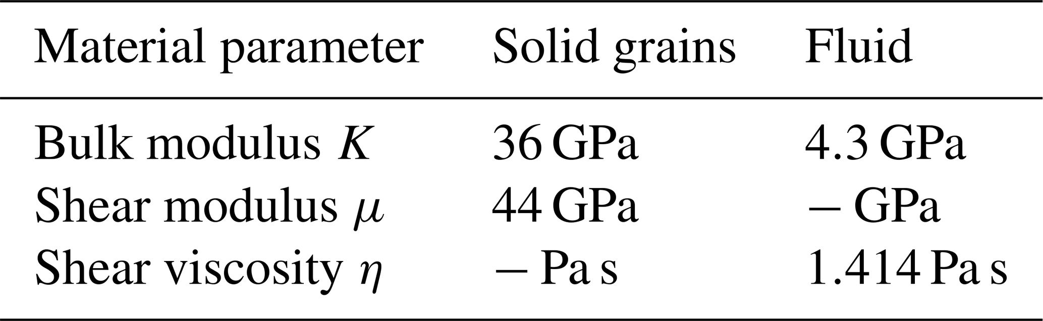
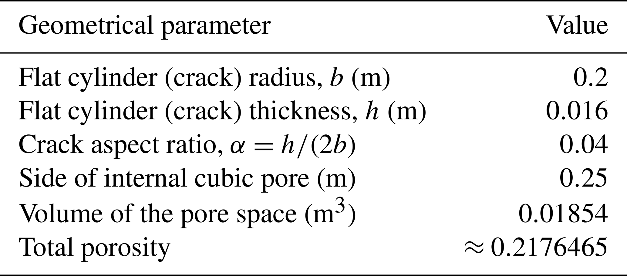
Alkhimenkov (2023) performed a numerical validation of Gassmann's equations considering a 3D numerical setup and relatively complex pore geometry that included narrow regions (cracks) and large pore space (Fig. 1a–b). The numerical model consisted of a solid phase representing the grain matrix and a pore space. The model was cubic, with dimensions of $\mathrm{0.44}\times \mathrm{0.44}\times \mathrm{0.44}\mathrm{m}$. The pore space comprised cracks, modeled as flat cylinders, connected to an internal cubic cavity, as illustrated in Fig. 1a–b. The material properties used in the simulations are listed in Table 1, while the geometrical characteristics of the pore space are provided in Table 2.

Table 1 Material properties used in all simulations.

Table 2 Geometrical properties of the model.

Alkhimenkov (2023) applied a 3D finite-element method to resolve the conservation of linear momentum coupled with the stress–strain relations for the solid phase and the quasi-static linearized compressible Navier–Stokes momentum equation for the fluid phase. The resulting system of equations was solved using a direct PARDISO solver (Schenk and Gärtner, 2004). Alkhimenkov (2023) conducted a convergence study showing that, for finer resolution, the result of the numerical solution converges towards the result obtained from the original Gassmann's equation. Such a convergence analysis validates the accuracy of Gassmann's equation for a particular (but arbitrary) pore geometry. Furthermore, the pore geometry that was used did not contain any special features (among all possible geometries) that were tailored to make it consistent with Gassmann's equations (Alkhimenkov, 2024). There are also other 3D numerical studies that consider different geometries of the pore space and that are consistent with Gassmann's equations (Alkhimenkov et al., 2020a, b; Alkhimenkov and Quintal, 2022a, b).

Here we extend the results of Alkhimenkov (2023) for a denser finite-element mesh (achieving 2 025 916 elements)) and report the convergence study showing that, for finer resolution, the result of the numerical solution converges towards the result obtained from the original Gassmann's equation (Fig. 1c–d).

10 Discussion

10.1 Physical interpretation of the present extended Biot's poroelastic framework

The derived extended Biot's poroelastic equations describe the coupled mechanical and fluid flow behavior of a fluid-saturated porous medium under general conditions. Specifically, they account for the interaction between solid matrix deformation and changes in pore fluid pressure. Classical Biot's equations (Biot, 1962) and Gassmann's equations (Gassmann, 1951) are special cases of the presented theory. Gassmann's equations provide a relation between the bulk moduli of the drained (or dry) and undrained fluid-saturated rock, offering insight into how fluid properties and porosity influence the mechanical response of the material.

10.2 Other derivations of Gassmann's equations

Gassmann's equations are directly related to the quasi-static formulation of poroelasticity developed by Biot (1941) and later extended to dynamic settings by Biot (1956, 1962). While the conceptual foundation of elastodynamic poroelasticity, such as the presence of the fast P-wave, slow P-wave, and shear wave in fluid-saturated porous media, was introduced by Frenkel (1944) (see also Pride and Garambois, 2005), rigorous derivations of the poroelastic parameters were provided subsequently by Biot (1941), Biot and Willis (1957), and Biot (1962).

Numerous researchers have re-derived Gassmann's equations using various approaches or examined specific aspects of these equations within the poroelasticity framework (Brown and Korringa, 1975; Rice and Cleary, 1976; Korringa, 1981; Burridge and Keller, 1981; Bourbié et al., 1987; Zimmerman, 1990; Berryman and Milton, 1991; Detournay and Cheng, 1993, Berryman, 1999; Smith et al., 2003; Lopatnikov and Cheng, 2004; Gurevich, 2007; Fortin and Guéguen, 2021). Some modifications of small-strain poroelasticity to include non-reciprocal effects are given by Sahay (2013) and Müller and Sahay (2019). While the full list of contributors to the field is extensive and beyond the scope of this paper, we acknowledge their foundational work.

We refer the reader to Sevostianov (2020), which presents a comprehensive overview of Gassmann's equations. In addition, several books may be useful for readers interested in poroelasticity and its applications, including Bourbié et al. (1987), Zimmerman (1990), Wang (2000), Ulm and Coussy (2003), Coussy (2004, 2011), Guéguen and Boutéca (2004), Dormieux et al. (2006), Cheng (2016), and Mavko et al. (2020).

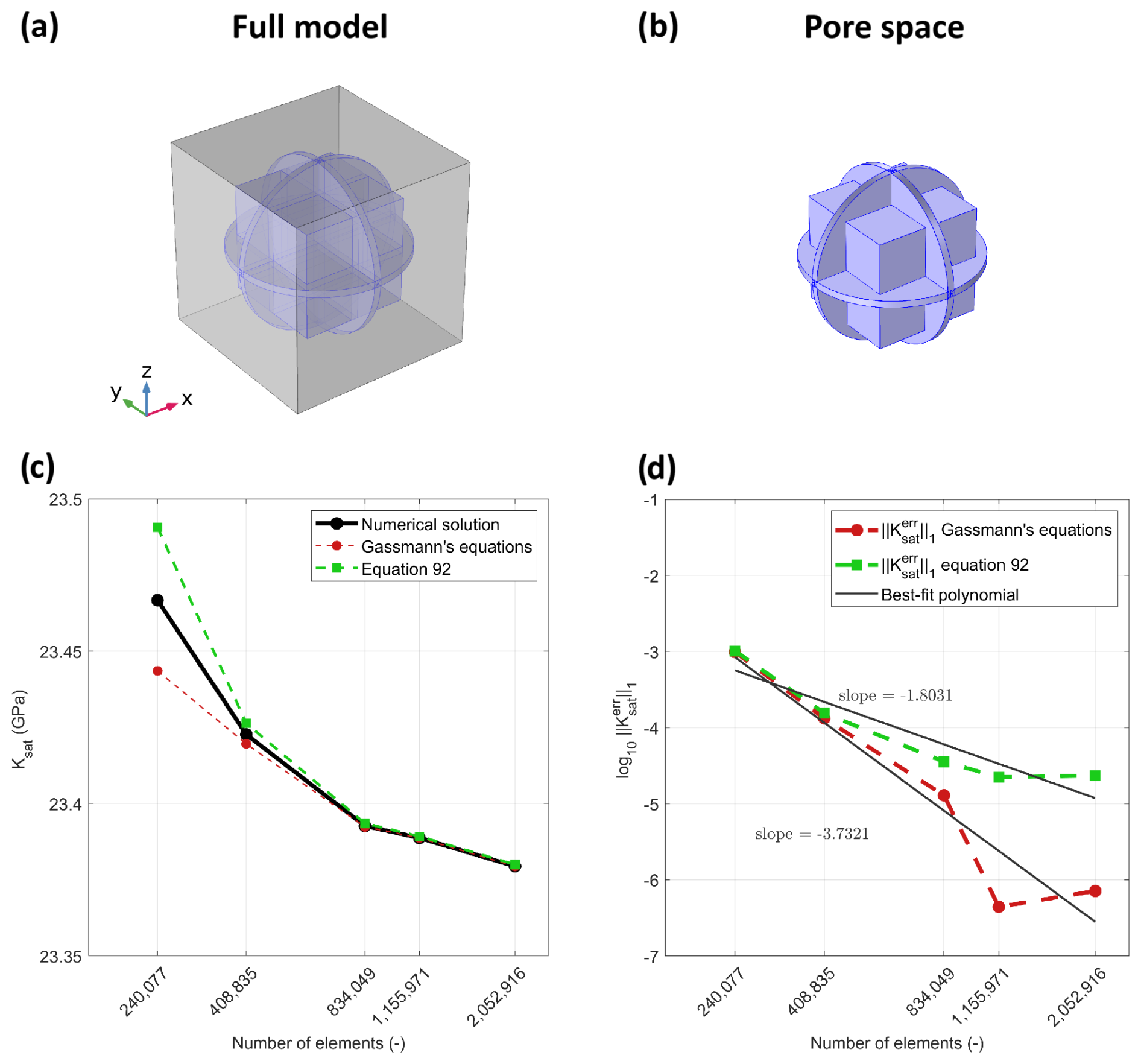
Figure 1 Panels (a)–(b) show sketches illustrating the model geometry. Panel (c) shows the numerical solution of K_u, the analytical solution via Gassmann's Eq. (47), and the analytical solution via Eq. (92) as a function of the numerical resolution. Panel (d) shows the error magnitudes between (i) the numerically evaluated bulk modulus K_u and the analytically evaluated bulk modulus via Gassmann's Eq. (47) and (ii) the numerically evaluated bulk modulus and the analytically evaluated bulk modulus via Eq. (92).

10.2.1 Thermodynamically admissible conditions for the diagonal structure of matrix H

The main assumptions behind the applicability of Gassmann's Eqs. (45)–(47) are (i) linear elasticity, (ii) small strains, (iii) an isotropic homogeneous frame material and isotropic homogeneous solid grains, (iv) an isotropic dry response (although Gassmann's original publication includes an extension to anisotropy), and (v) the self-similarity hypothesis: the assumption that equal changes in pore (fluid) pressure and confining (total) pressure leave the porosity unchanged (Korringa, 1981; Alkhimenkov, 2024).

Assumption (v) may hold for isotropic homogeneous frame materials (Korringa, 1981), but it must be derived rigorously. In the framework of the present study, this condition is satisfied when the compliance matrix H is diagonal, and it is required for the thermodynamic admissibility of the model (see Appendix B). As stated there: “the constraint of zero dissipation (entropy production) during reversible poroelastic deformation provides an essential constraint on the poroelastic constitutive equation for porosity evolution.”

10.2.2 When the solid compressibilities coincide (${\mathit{\beta }}_{\mathrm{s}}^{\prime \mathrm{EB}}={\mathit{\beta }}_{\mathrm{s}}^{\prime \prime \mathrm{EB}}={\mathit{\beta }}_{\mathrm{s}}={\mathit{\beta }}_{\mathrm{s}}^{\prime \mathrm{DC}}={\mathit{\beta }}_{\mathrm{s}}^{\prime \prime \mathrm{DC}}={\mathit{\beta }}_M^{\mathrm{BK}}={\underset{\mathrm{¯}}{\mathit{\beta }}}_S^{\mathrm{BK}}$)

Strictly speaking, the most general model should always use the full matrix H (Eq. 6). However, in certain special cases, such as isotropic and homogeneous rock frames, additional constraints may hold. Several researchers have pointed out that, for monomineralic isotropic materials, the self-similarity hypothesis is valid and that Gassmann's equations therefore apply and are exact (Brown and Korringa, 1975; Korringa, 1981).

In general, various poroelastic constants can be computed numerically (Alkhimenkov, 2023), derived analytically using effective medium theory (Yarushina and Podladchikov, 2015), or measured experimentally in laboratory settings (Makhnenko and Podladchikov, 2018).

The distinction between the solid compressibilities lies in the structure of the matrix H, which depends on the particular choice of rheological relationships. The definitions (Detournay and Cheng, 1993)

$$\begin{array}{}\text{(107)}& {\mathit{\beta }}_{\mathrm{s}}={\displaystyle \frac{\mathrm{1}}{K_{\mathrm{s}}}},{\mathit{\beta }}_{\mathrm{s}}^{\prime \mathrm{DC}}={\displaystyle \frac{\mathrm{1}}{K_{\mathrm{s}}^{\prime \mathrm{DC}}}},{\mathit{\beta }}_{\mathrm{s}}^{\prime \prime \mathrm{DC}}={\displaystyle \frac{\mathrm{1}}{K_{\mathrm{s}}^{\prime \prime \mathrm{DC}}}}\end{array}$$

are only necessary when the rock microstructure allows the bulk frame, solid grains, and pore space to deform differently under unjacketed loading (Makhnenko and Podladchikov, 2018) (K_s is the bulk modulus of solid grains). Note that the rheological assumptions in the Brown–Korringa (BK) model differ from those in the Detournay–Cheng (DC) and the presented extended Biot formulations. As a result, the interpretation and estimation of the parameters in Eq. (107) differ between models.

• The poroelastic parameters (Eq. 107) can be computed numerically with arbitrary precision. Numerical studies conducted in 3D confirm that, for isotropic (or cubic) monomineralic rock frames with isotropic grains and a fully interconnected pore space, the three parameters in Eq. (107) are equal (Alkhimenkov, 2023, 2024).

• These parameters can also be measured experimentally in laboratory settings, enabling practical application. In many practical situations, the differences between these parameters (Eq. 107) are small, and one can safely adopt a single solid modulus K_s. The condition ${\mathit{\beta }}_{\mathrm{s}}={\mathit{\beta }}_{\mathrm{s}}^{\prime \mathrm{DC}}={\mathit{\beta }}_{\mathrm{s}}^{\prime \prime \mathrm{DC}}$ typically holds when the rock has a monomineralic, isotropic, and uniform skeleton and a fully interconnected pore network and when it is subjected to pressures below the onset of micro-fracturing or mineral phase transitions. Under such assumptions, the unjacketed compression test measures the intrinsic mineral bulk modulus, and both the whole-specimen ($K_{\mathrm{s}}^{\prime \mathrm{DC}}$) and pore-volume ($K_{\mathrm{s}}^{\prime \prime \mathrm{DC}}$) moduli may collapse (as suggested by several studies) to $K_{\mathrm{s}}=\mathrm{1}/{\mathit{\beta }}_{\mathrm{s}}$, reducing the DC model to the original Biot–Gassmann formulation. That is, under unjacketed conditions, the entire solid surface is subjected to a uniform pressure increment Δp, and, if the rock is microscopically isotropic and homogeneous, both the solid grains and bulk framework undergo uniform volumetric strain, resulting in no change in porosity (Tarokh and Makhnenko, 2019). Typical examples include dense quartz sands, clean limestones below micro-crack initiation stress, and synthetic rock samples.

• Even for the multi-mineral skeleton, the differences between these parameters (Eq. 107) are small, which is shown in the 3D numerical study by Alkhimenkov (2025) and in laboratory settings (Makhnenko and Podladchikov, 2018).

• Finally, these parameters can also be derived using effective medium theory. This is the most rigorous way to establish under which conditions the three poroelastic parameters are equivalent. The application of effective medium theory is outside the scope of the present study but remains an important direction for future work.

We note that, when a rock frame consists of two or more minerals with different elastic properties (e.g., shales, poorly consolidated sandstones, or cracked carbonates), the distinction ${\mathit{\beta }}_M^{\mathrm{BK}}\ne {\underset{\mathrm{¯}}{\mathit{\beta }}}_S^{\mathrm{BK}}$ in the BK framework is present. In such cases, the assumptions underlying the self-similarity hypothesis break down, and Gassmann's equations serve only as a (very good) approximation within the framework of the extended Biot formulation (Alkhimenkov, 2025).

To further assess the magnitude of the off-diagonal components of the matrix H, we perform a Taylor expansion of ${\mathit{\beta }}_{\mathit{\delta }}^{\mathrm{EB}}={\mathit{\beta }}_{\mathrm{s}}^{\prime \mathrm{EB}}-{\mathit{\beta }}_{\mathrm{s}}^{\prime \prime \mathrm{EB}}$ (without imposing any assumption on mono- or multi-mineral composition of the frame):

$$\begin{array}{}\text{(108)}& \begin{array}{rl}& H_{\mathrm{1},\mathrm{2}}=\\ & {\displaystyle \frac{\mathrm{1}}{(\mathrm{1}-{\mathit{\varphi }}_{\mathrm{f}}{)}^{\mathrm{2}}\left(({\mathit{\beta }}_{\mathrm{s}}^{\prime \mathrm{EB}}{)}^{\mathrm{2}}+{\mathit{\beta }}_{\mathrm{d}}^{\mathrm{EB}}({\mathit{\varphi }}_{\mathrm{f}}-\mathrm{2}){\mathit{\beta }}_{\mathrm{s}}^{\prime \mathrm{EB}}+{\mathit{\beta }}_{\mathrm{d}}^{\mathrm{EB}}{\mathit{\beta }}_{\mathrm{s}}^{\prime \mathrm{EB}}\right)}}\\ & \cdot {\mathit{\beta }}_{\mathit{\delta }}^{\mathrm{EB}}+O\left({\mathit{\beta }}_{\mathit{\delta }}^{\mathrm{2}}\right),\end{array}\end{array}$$

which demonstrates that the off-diagonal terms of H are small.

10.3 Comparison of Gassmann's equations and Thomsen's alternative formulation

Thomsen (2023b) argued that the original derivation of Gassmann's equations contains a logical error, namely an incorrect application of Love's theorem to hydraulically open and closed systems. In the present derivation, we rely on classical irreversible thermodynamics and do not rely on any assumptions regarding whether the porous material system is open or closed.

Thomsen (2023b) provided an updated version of these relations (see also Brown and Korringa, 1975):

$$\begin{array}{}\text{(109)}& K_{\mathrm{u}}=K_{\mathrm{d}}+{\displaystyle \frac{{\left(\mathrm{1}-K_{\mathrm{d}}(K_M^{\mathrm{BK}}{)}^{-\mathrm{1}}\right)}^{\mathrm{2}}}{{\mathit{\varphi }}_{\mathrm{f}}{K}_{\mathrm{f}}^{-\mathrm{1}}+(\mathrm{1}-{\mathit{\varphi }}_{\mathrm{f}}){\underset{\mathrm{¯}}{K}}_{\mathrm{s}}^{-\mathrm{1}}-K_{\mathrm{d}}^{\mathrm{BK}}/(K_M^{\mathrm{BK}}{)}^{\mathrm{2}}}},\end{array}$$

where $K_M^{\mathrm{BK}}$ is a new parameter referred to as the “mean” bulk modulus (Thomsen, 2023b). Note the similarity between expressions (47) and (109). Thomsen's relation introduces one additional parameter, $K_M^{\mathrm{BK}}$, beyond the original Gassmann Eq. (47). Thomsen (2023b) also provided ways to evaluate $K_M^{\mathrm{BK}}$, including

$$\begin{array}{}\text{(110)}& K_M^{\mathrm{BK}}={\left[{\displaystyle \frac{\mathrm{1}}{K_{\mathrm{d}}^{\mathrm{BK}}}}-{\displaystyle \frac{\mathrm{1}}{B^{\mathrm{BK}}}}\left({\displaystyle \frac{\mathrm{1}}{K_{\mathrm{d}}^{\mathrm{BK}}}}-{\displaystyle \frac{\mathrm{1}}{K_{\mathrm{u}}^{\mathrm{BK}}}}\right)\right]}^{-\mathrm{1}},\end{array}$$

where B^BK (Skempton coefficient) is directly observable in quasi-static experiments. Alternatively, expression (110) can be rewritten as

$$\begin{array}{}\text{(111)}& K_M^{\mathrm{BK}}={\left[{\displaystyle \frac{\begin{array}{c}{B}^{\mathrm{BK}}\left({\mathit{\varphi }}_{\mathrm{f}}{K}_{\mathrm{f}}^{-\mathrm{1}}+(\mathrm{1}-{\mathit{\varphi }}_{\mathrm{f}})({\underset{\mathrm{¯}}{K}}_{\mathrm{s}}^{\mathrm{BK}}{)}^{-\mathrm{1}}\right)\\ -(\mathrm{1}-B^{\mathrm{BK}})(K_{\mathrm{d}}^{\mathrm{BK}}{)}^{-\mathrm{1}}\end{array}}{\mathrm{2}{B}^{\mathrm{BK}}-\mathrm{1}}}\right]}^{-\mathrm{1}}.\end{array}$$

Importantly, Thomsen's formulation reduces to Gassmann's when $K_M^{\mathrm{BK}}={\underset{\mathrm{¯}}{K}}_S^{\mathrm{BK}}$.

Thomsen (2023b) argued that this additional parameter $K_M^{\mathrm{BK}}$ must be independently measured, even for monomineralic rocks, and that Eq. (109) should be used instead of the original Gassmann relation (47). As follows from Eq. (111), evaluating $K_M^{\mathrm{BK}}$ requires an independent measurement of the Skempton coefficient B^BK. Thomsen (2023b) further noted that the porosity ϕ_f is not constant under equal changes in fluid pressure p_f and total pressure $\overline{p}$ and argued that, for monomineralic rocks, $K_M^{\mathrm{BK}}$ generally differs from ${\underset{\mathrm{¯}}{K}}_S^{\mathrm{BK}}$. This implies a sensitivity of porosity variation, either increasing or decreasing, depending on the sign of $K_M^{\mathrm{BK}}-{\underset{\mathrm{¯}}{K}}_S^{\mathrm{BK}}$.

We note the following:

• Gassmann explicitly stated the self-similarity hypothesis in his original article (Gassmann, 1951). Therefore, claims of a logical error (Thomsen, 2023b) in the derivation are unfounded.

• The claims made by Thomsen (2023b) are not supported by rigorous theoretical developments (e.g., exact solutions in effective medium theory) that explicitly demonstrate that $K_M^{\mathrm{BK}}\ne {\underset{\mathrm{¯}}{K}}_S^{\mathrm{BK}}$ for monomineralic rocks.

• Several 3D numerical studies confirm that the self-similarity hypothesis holds for homogeneous isotropic (or cubic) dry responses and isotropic solid-grain materials. This has been verified numerically for both cubic and transversely isotropic symmetries (Alkhimenkov et al., 2020a, b; Alkhimenkov and Quintal, 2022a, b; Alkhimenkov, 2023, 2024).

• A recent 3D numerical study of a heterogeneous frame material composed of two solids with different bulk and shear moduli (Alkhimenkov, 2025) showed that the difference $K_M^{\mathrm{BK}}-{\underset{\mathrm{¯}}{K}}_S^{\mathrm{BK}}$ is below 0.11 GPa, practically insignificant.

• Laboratory experiments show that, even for the multi-mineral skeleton, the differences between $K_M^{\mathrm{BK}}$ and ${\underset{\mathrm{¯}}{K}}_S^{\mathrm{BK}}$ are small (Makhnenko and Podladchikov, 2018).

• This all suggests that, in relatively homogeneous rock samples, the distinction between different solid-grain moduli has negligible practical impact.

• The mechanics of rocks includes additional important aspects such as nonlinearity in their mechanical response, differences in mechanical properties under extension versus compression (which can differ by several percent), intrinsic anisotropy of the solid grains, effective anisotropy of the rock sample, and irreversible damage under applied loads. All of these factors contribute to a much more complex mechanical behavior of rocks. These additional constraints may have a significantly greater impact on rock response than potential deviations from the self-similarity hypothesis.

Alkhimenkov (2023) conducted a numerical convergence study demonstrating that $K_M^{\mathrm{BK}}\to K_{\mathrm{s}}$ (where K_s is the solid bulk modulus) for monomineralic rock as the resolution increases. In this study, $K_M^{\mathrm{BK}}$ was computed independently using Eq. (111), with the Skempton coefficient B^BK also calculated. Consequently, the result of expression (109) converges to the original Gassmann relation (47) in the monomineralic isotropic (or cubic symmetry) case where $K_M^{\mathrm{BK}}\equiv K_{\mathrm{s}}$ (within numerical precision), thereby validating the original Gassmann formulation for a particular pore space and solid material geometry.

10.4 Limitations

Often, natural rocks are composed of multiple minerals that are anisotropic, and they typically exhibit some degree of intrinsic anisotropy. They may also contain a combination of compliant cracks (e.g., grain contacts) and stiff pores, which respond differently under mechanical loading. Additionally, a rock's heterogeneity can violate the assumptions of a representative volume element. It is also well established that elastic moduli can vary by several percent under compression versus extension. These deviations from ideal small-strain elasticity suggest the need for additional effective parameters, and thus more experimental (or numerical) measurements, to accurately characterize fully saturated and realistic rock samples.

11 Conclusions

This study has presented a structured, transparent, and thermodynamically admissible derivation of the quasi-static extended Biot's poroelasticity framework. The well-known classical Gassmann equations and Biot poroelastic formulation (fundamental tools for characterizing the poroelastic mechanical behavior of fluid-saturated porous media) are derived here as special cases of the general theory. While the thermodynamic admissibility of the original Biot equations has previously been demonstrated, the present work extends this admissibility to a more general model using the framework of classical irreversible thermodynamics. We emphasize clarity, accessibility, and full reproducibility throughout the derivation. The main novelty of this study is the development of the extended Biot's poroelasticity framework, which incorporates off-diagonal components of the Hessian matrix. The relations between the new set of poroelastic parameters are fully expressed in terms of the components of the Hessian matrix H.

By strictly adhering to conservation laws and thermodynamic principles, we have also addressed recent claims by Leon Thomsen regarding the validity of Gassmann's formulation. In particular, we have shown that the key self-similarity assumption (that porosity remains unchanged under equal changes in fluid and total pressure) is a sufficient but unnecessary condition for the derivation of a Gassmann-type relationship between undrained and drained bulk moduli. Indeed the extended Gassmann poroelastic Eq. (69) is derived in this contribution without relying on Gassmann's assumption of self-similarity.

To promote transparency and support future developments, we provide symbolic Maple routines. These materials ensure full reproducibility of the derivations and offer a practical foundation for extending the framework to more complex scenarios, such as multiphase fluid systems and related phenomena.

Appendix A: Explanation of the Maple script for a single-phase medium

The following Maple script provides a step-by-step derivation of the entropy production for a one-dimensional system using the principles of classical irreversible thermodynamics. It uses the volume-specific formulation for mass conservation and the principles of local thermodynamic equilibrium (LTE) to establish the relationship between different thermodynamic fluxes and forces. The script calculates the entropy production, Q[s], and demonstrates the impact of various choices for flux definitions. Below is a detailed explanation of each step in the script.

Listing A1 Maple script for entropy production.

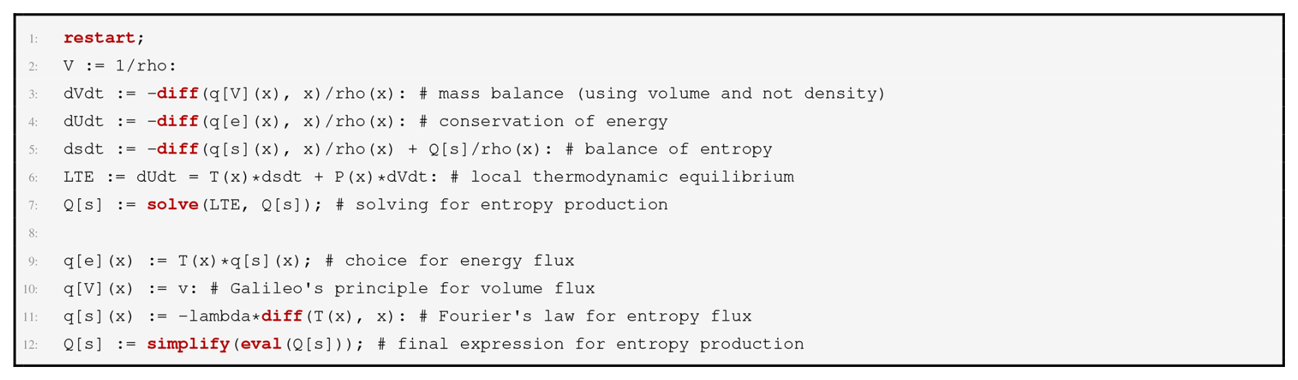
Below, we provide a detailed explanation of each line in the script.

Initialization and mass conservation

Listing A2 Here, V is defined as the specific volume, which is the inverse of density, ρ.

Listing A3 This line represents the mass conservation equation using the volume-specific formulation. It calculates the time derivative of the specific volume as the negative divergence of the volume flux q[V](x) divided by the local density.

Conservation of energy

Listing A4 This represents the conservation of energy, where dUdt is the time derivative of the specific internal energy and q[e](x) is the energy flux. The equation states that the change in internal energy is equal to the negative divergence of the energy flux divided by the density.

Entropy balance

Listing A5 This line represents the entropy balance. Here, dsdt is the time derivative of specific entropy, q[s](x) is the entropy flux, and Q[s] is the entropy production rate per unit volume. This equation states that the change in entropy is equal to the negative divergence of the entropy flux plus the entropy production term.

Local thermodynamic equilibrium (LTE)

Listing A6 This equation expresses the principle of local thermodynamic equilibrium (LTE). It relates the internal energy change dUdt to the product of temperature T(x) and entropy change dsdt, plus the product of pressure P(x) and volume change dVdt.

Solving for entropy production

Listing A7 The script solves the LTE equation for the entropy production term Q[s].

Choice for energy flux

Listing A8 The energy flux q[e](x) is chosen as the product of temperature T(x) and entropy flux q[s](x). This is a common assumption based on the linear coupling between the energy and entropy fluxes.

Flux definitions

Listing A9 The volume flux q[V](x) is represented by velocity v following Galileo's principle. The entropy flux q[s](x) is defined according to Fourier's law, where it is proportional to the temperature gradient diff(T(x), x) with thermal conductivity lambda.

Final expression for entropy production

The final expression for entropy production Q[s] is simplified to

$$\begin{array}{}\text{(A1)}& Q\left[s\right]={\displaystyle \frac{\mathit{\lambda }}{T\left(x\right)}}{\left({\displaystyle \frac{\mathrm{d}T\left(x\right)}{\mathrm{d}x}}\right)}^{\mathrm{2}}.\end{array}$$

Listing A10 This result shows that the entropy production is non-negative and is proportional to the square of the temperature gradient, divided by temperature, which is a classical result in non-equilibrium thermodynamics.

Appendix B: Explanation of the Maple script for two-phase fluid-saturated media

B1 General representation of classical irreversible thermodynamics

Porous materials can be modeled as two-phase systems composed of a solid skeleton and a saturating fluid. These phases exchange mass, momentum, and energy, leading to complex coupled processes that are naturally described using the framework of classical irreversible thermodynamics (CIT) (Gyarmati, 1970; Jou et al., 1996; Lebon et al., 2008; Yarushina and Podladchikov, 2015). In this formulation, conservation equations for mass, momentum, entropy, and energy are expressed in the Eulerian frame as follows:

$$\begin{array}{}\text{(B1)}& {\displaystyle \frac{\partial \left(\mathit{\rho }\mathit{\varphi }\right)}{\partial t}}+{\mathrm{\nabla }}_j\left(\mathit{\rho }\mathit{\varphi }{\mathit{v}}_j+q_{\mathit{\rho }}^j\right)=Q_p,\text{(B2)}& {\displaystyle \frac{\partial \left(\mathit{\rho }\mathit{\varphi }{\mathit{v}}_i\right)}{\partial t}}+{\mathrm{\nabla }}_j\left(\mathit{\rho }\mathit{\varphi }{\mathit{v}}_i{\mathit{v}}_j+q_{\mathit{v}}^{ij}\right)=Q_{v_i},\text{(B3)}& {\displaystyle \frac{\partial \left(\mathit{\rho }\mathit{\varphi }\mathit{s}\right)}{\partial t}}+{\mathrm{\nabla }}_j\left(\mathit{\rho }\mathit{\varphi }\mathit{s}{\mathit{v}}_j+q_{\mathit{s}}^j\right)=Q_s,\text{(B4)}& {\displaystyle \frac{\partial \left(\mathit{\rho }\mathit{\varphi }\mathit{e}\right)}{\partial t}}+{\mathrm{\nabla }}_j\left(\mathit{\rho }\mathit{\varphi }\mathit{e}{\mathit{v}}_j+q_{\mathit{e}}^j\right)=Q_{\mathrm{e}},\end{array}$$

where v_j, s, and e denote the velocity, specific entropy, and specific total energy per unit mass, respectively. The term ρ denotes (phase-specific) density, and ϕ denotes the phase volume fraction (e.g., porosity for the fluid). The term ∇_j representsthe partial derivative with respect to spatial coordinates, while $q_{\mathit{\rho }}^j$, $q_{\mathit{v}}^{ij}$, $q_{\mathit{s}}^j$, and $q_{\mathit{e}}^j$ correspond to the fluxes of mass, momentum, entropy, and energy, respectively. The terms Q_p, $Q_{v_i}$, Q_s, and Q_e represent the corresponding production rates due to irreversible processes (Yarushina and Podladchikov, 2015).

Entropy production (TQ_s)

Solving the local entropy production equation for Q_s and multiplying both sides by the absolute temperature T, we obtain

$$\begin{array}{}\text{(B5)}& \begin{array}{rl}T{Q}_{\mathrm{s}}& =\mathit{\eta }\mathit{\varphi }{\left({\displaystyle \frac{\mathrm{d}v}{\mathrm{d}x}}\right)}^{\mathrm{2}}+{\displaystyle \frac{\mathit{\lambda }\mathit{\varphi }}{T}}{\left({\displaystyle \frac{\mathrm{d}T}{\mathrm{d}x}}\right)}^{\mathrm{2}}+pv{\displaystyle \frac{d\mathit{\varphi }}{\mathrm{d}x}}-v{Q}_v\\ & -Q_{\mathit{\rho }}{G}_{\text{Gibbs}}+Q_{\mathrm{u}}+p{\displaystyle \frac{\mathrm{d}\mathit{\varphi }}{\mathrm{d}t}}-{\mathit{\tau }}_{\mathit{\varphi }}{\displaystyle \frac{\mathrm{d}{\mathit{\varphi }}^{\mathrm{e}}}{\mathrm{d}t}}.\end{array}\end{array}$$

This expression represents the entropy production, which must be non-negative according to the second law of thermodynamics. Notably, this formulation assumes local thermodynamic equilibrium separately for the solid and fluid phases. This is a weaker assumption than Biot's original model (Biot, 1962), which postulated a single internal energy potential for the entire two-phase system in the linear poroelastic regime (Yarushina and Podladchikov, 2015).

B2 Thermodynamic constraints on fluxes and productions

CIT requires that the total entropy production of the system remains non-negative. This condition applies both to the intra-phase and inter-phase entropy production within a porous medium. Mathematically, this is expressed as

$$\begin{array}{}\text{(B6)}& \sum _{\text{phases}}{Q}_{\mathrm{s}}=\sum _{\text{phases}}{Q}_{\mathrm{s}}^{\text{intra}}+Q_{\mathrm{s}}^{\text{inter}}\ge \mathrm{0}.\end{array}$$

Here, $Q_{\mathrm{s}}^{\text{intra}}$ represents the intra-phase entropy production within each phase (e.g., due to viscosity, heat conduction, or internal diffusion), while $Q_{\mathrm{s}}^{\text{inter}}$ represents the entropy production arising from inter-phase interactions (e.g., interactions between the solid skeleton and the fluid phase). To satisfy CIT, each contribution must be non-negative:

$$\begin{array}{}\text{(B7)}& Q_{\mathrm{s}}^{\text{intra}}\ge \mathrm{0},Q_{\mathrm{s}}^{\text{inter}}\ge \mathrm{0}.\end{array}$$

B3 Extended thermodynamic admissibility

Building on the principles of classical irreversible thermodynamics (CIT) (Lebon et al., 2008) and the nonlinear viscoelastoplastic framework of Yarushina and Podladchikov (2015), the derivation of the extended Biot poroelastic equations must satisfy the conditions of thermodynamic admissibility. Specifically, the entropy production Q_s must remain non-negative, and the constitutive relations must be formulated such that they are consistent with the second law of thermodynamics for all admissible thermodynamic paths.

From Eq. (37), and taking into account the requirement that entropy production must be non-negative, the inelastic porosity equation takes the form (Yarushina and Podladchikov, 2015)

$$\begin{array}{}\text{(B8)}& {\displaystyle \frac{{\mathrm{d}}^{\mathrm{s}}{\mathit{\varphi }}_{\mathrm{f}}}{\mathrm{d}t}}-{\displaystyle \frac{{\mathrm{d}}^{\mathrm{s}}{\mathit{\varphi }}_{\mathrm{f}}^{\mathrm{e}}}{\mathrm{d}t}}=-{\displaystyle \frac{p_{\mathrm{e}}}{{\mathit{\eta }}_{\mathit{\varphi }}}},\end{array}$$

where η_ϕ stands for the effective bulk viscosity. After simplifying and collecting terms (see Appendix B), the total entropy production becomes

$$\begin{array}{}\text{(B9)}& \begin{array}{rl}T{Q}_{s,\text{total}}& ={\displaystyle \frac{\mathrm{1}}{{\mathit{\eta }}_{\mathit{\varphi }}}}{\left({\displaystyle \frac{p_{\mathrm{e}}}{(\mathrm{1}-{\mathit{\varphi }}_{\mathrm{f}})}}\right)}^{\mathrm{2}}+{\mathit{\eta }}_{\mathrm{t}}{\left(\mathrm{\nabla }\cdot v^{\mathrm{s}}\right)}^{\mathrm{2}}\\ & +{\displaystyle \frac{(q^D{)}^{\mathrm{2}}{\mathit{\eta }}_{\text{dV}}}{{\mathit{\varphi }}_{\mathrm{f}}}}+{\displaystyle \frac{{\mathit{\lambda }}_{\mathrm{t}}}{T}}{\left({\displaystyle \frac{\partial T}{\partial x}}\right)}^{\mathrm{2}}.\end{array}\end{array}$$

• ${\displaystyle \frac{\mathrm{1}}{{\mathit{\eta }}_{\mathit{\varphi }}}}{\left({\displaystyle \frac{p_{\mathrm{e}}}{(\mathrm{1}-{\mathit{\varphi }}_{\mathrm{f}})}}\right)}^{\mathrm{2}}$: entropy production due to poroviscous deformation (effective viscosity η_ϕ and effective pressure $p_{\mathrm{e}}=\overline{p}-p_{\mathrm{f}}$).

• ${\mathit{\eta }}_{\mathrm{t}}{\left(\mathrm{\nabla }\cdot v^{\mathrm{s}}\right)}^{\mathrm{2}}$: entropy production due to viscous dissipation in the solid phase.

• ${\displaystyle \frac{(q^D{)}^{\mathrm{2}}{\mathit{\eta }}_{\text{dV}}}{{\mathit{\varphi }}_{\mathrm{f}}}}$: entropy production due to viscous dissipation in fluid flow (Darcy flow).

• ${\displaystyle \frac{{\mathit{\lambda }}_{\mathrm{t}}}{T}}{\left({\displaystyle \frac{\partial T}{\partial x}}\right)}^{\mathrm{2}}$: entropy production due to heat conduction (Fourier's law).

The non-negative nature of each term ensures the overall positivity of entropy production, thereby confirming the thermodynamic validity of the system of extended Biot's poroviscoelastic equations.

A more detailed derivation is given below (see also the discussions provided by Yarushina and Podladchikov, 2015). Additionally, symbolic Maple routines used to reproduce and validate the theoretical results presented in this article are available in a permanent DOI repository (Zenodo) (Alkhimenkov and Podladchikov, 2024).