Understanding seismic anisotropy in the Rotondo granite: investigating stress as a potential source

The hypothesis of stress-induced seismic anisotropy was tested in the Bedretto Lab, a deep underground rock laboratory in the Swiss Alps. Several comprehensive cross-hole seismic surveys were acquired to analyze the directional dependency of seismic-wave velocities in the undisturbed host rock. This requires precise knowledge on the source and receiver positions as well as good data quality that allows the determination of travel times for different wave types. A tilted transverse isotropic (TTI) model that explains the measured data to a first-order approximation can be established. All relevant model parameters are well constrained using P- and S-wave arrival times. However, a systematic misfit distribution indicates that a more complex anisotropy model might be required to fully explain the measurements. This is consistent with our hypothesis that seismic anisotropy has a significant stress-induced component. More controlled laboratory experiments on the centimeter to decimeter scale were performed to validate our field measurements. These measurements show a comparable order of P- and S-wave anisotropy in the rock volume. The knowledge on the driving mechanism for anisotropy in igneous rocks can potentially help to enhance the monitoring of stress field variations during geothermal operations, thereby improving hazard assessment protocols.

1 Introduction

The importance of seismic anisotropy, hereafter referred to as anisotropy, is well known and has been studied for decades. Neglecting anisotropy in seismic imaging can result in significant errors in terms of travel time calculations and ray path determinations. Examples on an exploration scale include Eken et al. (2012), Daley and Hron (1977), and Thomsen (1986). In engineering applications, it is important to consider anisotropy as it affects the stability of excavations and boreholes, rock-cutting performance, and fracture propagation (Heng et al., 2015; Lee et al., 2012; Özbek et al., 2018). Beyond this, anisotropy should not only be considered to describe the in situ state of a rock volume, but it can also help to monitor changes over time (Crampin and Booth, 1989; Gerst and Savage, 2004).

Aligned minerals, foliation, fractures, faults, bedding of a rock, and the in situ stress field are known to cause seismic anisotropy in rocks (Barton, 2006; Al-Harthi, 1998; Song et al., 2004; Chan and Schmitt, 2015; Nur and Simmons, 1969; Sayers, 2002). The type of rock (sedimentary, igneous, or metamorphic) and the considered scale are decisive to determine which parameters control the elastic behavior of the rock. Anisotropy of sedimentary rocks is often controlled by the internal bedding of the rock or alignment of minerals, while metamorphic rocks often show a foliation depending on the stress field while the rock was formed (Horne, 2013; Thomsen, 1986; Heng et al., 2015; Özbek et al., 2018). The controlling parameter can also vary on different scales, so a fault zone can be the dominant feature on a regional scale, but mineral alignment can control the wave propagation on smaller samples of the same rock volume.

Nevertheless, it can be very valuable to overcome this challenge and characterize the source of a present anisotropy. Its variation in space and time gives important insights into ongoing processes in the rock, especially if the anisotropy is stress induced. It can help to identify processes such as fracture opening or depressurization of magmatic systems and can therefore be used to observe and predict complex system behavior such as volcanic eruptions or geothermal energy extraction (Johnson et al., 2011; Crampin and Booth, 1989).

Most anisotropy studies have been carried out on sedimentary or metamorphic rocks, as these rock types are expected to have higher anisotropy (Al-Harthi, 1998). However, igneous rocks can also have a significant anisotropy, which should be incorporated, especially if the rocks are jointed or disturbed by fault zones (Ramamurthy et al., 1993). While both the source of anisotropy and the direction of the faster velocity are often obvious in sedimentary or metamorphic rocks, it might be harder to detect the symmetry direction and controlling parameters in igneous rocks. It becomes even more difficult when the controlling mechanism varies locally or regionally, as is often the case in heterogeneous rock volumes (Li and Peng, 2017; Johnson et al., 2011).

In our study, we analyze the anisotropy of an undisturbed igneous rock in an underground laboratory. Such laboratories provide the opportunity for field-scale in situ experiments to understand processes relevant to geoenergy, nuclear waste disposal, earthquake nucleation, or engineering aspects (Plenkers et al., 2023; Ma et al., 2022). All these potential applications can benefit from the realistic scale that such laboratories offer (compared to small-scale laboratory experiments) (Gischig et al., 2020). In addition, we can compare our results with previous analyses on the geology, fracture network, and stress field around the test volume. The link of the anisotropy to fractures and stress is especially highly important for the characterization of a geothermal reservoir, as these parameter control the reservoir creation and fluid flow during geothermal production (Amann et al., 2018). In this contribution, we characterize the anisotropy of the rock volume of interest by active seismic measurements in three differently oriented boreholes. We evaluate the known sources of anisotropy by comparing our results to the other measurement campaigns and identify the controlling parameter in the undisturbed igneous rock.

The paper is structured as follows. In the first part, the required theory used to describe the anisotropy is explained. Then the laboratory itself and the performed measurement campaigns are introduced. The last part explains and analyzes the resulting model, and the results are discussed in a bigger context, comparing our results with other data sets.

2 Theory

The commonly studied type of anisotropy in earth's structures is a (tilted) transverse isotropic medium (TTI) (Aminzadeh et al., 2022; Horne, 2013). Such a medium is characterized by a velocity v₀, given in m s⁻¹, in the direction of a symmetry axis and a rotationally symmetric velocity distribution around it, resulting in a symmetry plane of (usually) higher velocity perpendicular to it. Lower symmetries, such as the orthorhombic symmetry, introduce more complexity to the system but also increase the number of unknowns drastically (Tsvankin, 1997). A TTI medium, or hexagonal material, is one of the simplest forms of anisotropy that can be used in geophysical applications and is well studied (Carcione et al., 1988; Thomsen, 1986). We therefore start approximating our measurement data with a TTI medium.

The mathematical framework to describe such a medium is given, for example, in Daley and Hron (1977). They state that the velocity field in a TTI medium can be fully described by the five independent parameters C_ij of the elastic tensor, given in pascals (Pa), and the density of the rock ρ, given in kilograms per cubic meter (kg m⁻³). For the calculation of the velocity in a specific direction, the inclination angle ξ, given in radians (rad), between the wave front normal and the symmetry axis must also be known. The normal wave front can be described by the azimuth φ_r and the dip θ_r from the source to the receiver. So in addition to the unknown elastic tensor parameters C_ij, the orientation of the tensor itself in the principal coordinate system is also unknown in our case. The orientation of the tensor can be described by the azimuth φ₀ and the dip θ₀ of the symmetry axis.

The phase velocities of the different wave types are then defined as

$$\begin{array}{}\text{(1)}& {\displaystyle }{v}_{\mathrm{P}}\left(\mathit{\xi }\right)=\sqrt{{\displaystyle \frac{\mathrm{1}}{\mathrm{2}\mathit{\rho }}}[C_{\mathrm{33}}+C_{\mathrm{55}}+(C_{\mathrm{11}}-C_{\mathrm{33}}\left){\sin }^{\mathrm{2}}\right(\mathit{\xi })+D(\mathit{\xi }\left)\right]},\text{(2)}& {\displaystyle }{v}_{\mathrm{S}\mathrm{1}}\left(\mathit{\xi }\right)=C_{\mathrm{66}}{\sin }^{\mathrm{2}}\left(\mathit{\xi }\right)+C_{\mathrm{55}}{\cos }^{\mathrm{2}}\left(\mathit{\xi }\right),\text{(3)}& {\displaystyle }{v}_{\mathrm{S}\mathrm{2}}\left(\mathit{\xi }\right)=\sqrt{{\displaystyle \frac{\mathrm{1}}{\mathrm{2}\mathit{\rho }}}[C_{\mathrm{33}}+C_{\mathrm{55}}+(C_{\mathrm{11}}-C_{\mathrm{33}}\left){\sin }^{\mathrm{2}}\right(\mathit{\xi })-D(\mathit{\xi }\left)\right]},\end{array}$$

with

$$\begin{array}{}\text{(4)}& \begin{array}{rl}D\left(\mathit{\xi }\right)=& \left[\right(C_{\mathrm{33}}-C_{\mathrm{55}}{)}^{\mathrm{2}}+\mathrm{2}\left[\mathrm{2}\right(C_{\mathrm{13}}+C_{\mathrm{55}}{)}^{\mathrm{2}}\\ & -(C_{\mathrm{33}}-C_{\mathrm{55}})(C_{\mathrm{11}}+C_{\mathrm{33}}-\mathrm{2}{C}_{\mathrm{44}})\left]{\sin }^{\mathrm{2}}\right(\mathit{\xi })\\ & +\left[\right(C_{\mathrm{11}}+C_{\mathrm{33}}-\mathrm{2}{C}_{\mathrm{44}}{)}^{\mathrm{2}}-\mathrm{4}(C_{\mathrm{13}}+C_{\mathrm{55}}{)}^{\mathrm{2}}]{\sin }^{\mathrm{4}}\left(\mathit{\xi }\right){]}^{\mathrm{1}/\mathrm{2}}\end{array}.\end{array}$$

The elastic parameters C_ij can also be expressed by the Thomsen parameters α₀, β₀, γ, ϵ, and δ. These parameters are defined by Thomsen (1986) as follows:

• α₀ is the P-wave velocity along the symmetry axis $\sqrt{C_{\mathrm{33}}/\mathit{\rho }}$,

• β₀ is the S-wave velocity along the symmetry axis $\sqrt{C_{\mathrm{55}}/\mathit{\rho }}$,

• γ is the fractional difference between vertical and horizontal S1-wave velocity $(C_{\mathrm{66}}-C_{\mathrm{55}})/\mathrm{2}{C}_{\mathrm{55}}$,

• δ is the controlling parameter for rays subparallel to the symmetry axis
  $\left(\right(C_{\mathrm{13}}+C_{\mathrm{55}}{)}^{\mathrm{2}}-(C_{\mathrm{33}}-C_{\mathrm{55}}{)}^{\mathrm{2}})/\left(\mathrm{2}{C}_{\mathrm{33}}\right(C_{\mathrm{33}}-C_{\mathrm{55}}\left)\right)$, and

• ϵ is the fractional difference between vertical and horizontal P-wave velocity $(C_{\mathrm{11}}-C_{\mathrm{33}})/\mathrm{2}{C}_{\mathrm{33}}$.

The advantage of these parameters is that they have a direct physical meaning and are much easier to interpret than the elastic tensor parameters. We use Eqs. (1) to (3), with C_ij expressed by the Thomsen parameters to describe the velocities in our medium.

It is important to mention two major differences between the wave propagation in an isotropic and an anisotropic medium. First, the group and phase velocities and angles are not the same in an anisotropic medium (Thomsen, 1986). The energy of a signal propagates along the ray (group angle) with the group velocity, while Eqs. (1) to (3) describe the phase velocity along the wave front normal (phase angle). Second, the S-wave velocity does not only depend on its propagation direction but also on its polarization direction. This causes a splitting of the S wave in a fast wave and in a slow wave, described by Eqs. (2) and (3). This splitting clearly indicates that the medium of interest is anisotropic.

We assume that the velocity distribution in the medium of interest is sufficiently homogeneous, such that a straight ray assumption is justified. Also, the phase and group velocity directions can be assumed to be the same in our case of weak anisotropy and the assumption of straight rays (Wang et al., 2017; Berryman, 1979). Thus, we can calculate the predicted travel times by dividing the distance based on the known source and receiver positions by the apparent velocities along the straight ray.

We minimize the weighted L2 norm of the different waveforms to determine the Thomsen parameters of our medium of interest. For this purpose, we consider the first arriving P waves and the arrival of both the faster S wave and the slower S wave. The arrival times of the P waves are more accurate than the corresponding S waves. We therefore weight the L2 norm of the P-wave misfit higher compared to the L2 norm of the different S waves. With this, we ensure that the resulting model is not biased by outliers in the S-wave picks.

The reliability of the estimated Thomsen parameters is important for the interpretation of the results. This reliability can be estimated with tools from linear inverse theory. Here, we consider the model resolution matrix R, relating the true model parameter m^true to the estimated parameter m^est. The relative values on the diagonal of R give an estimate of how well we can determine the different parameters. The off-diagonal values show trade-offs between the different parameters and thus reveal dependencies between the model parameters.

We follow the definition of Menke (2018) to calculate $\mathbf{R}=({\mathbf{G}}^{\mathrm{T}}\mathbf{G}+\mathit{\lambda }\mathbb{1}{)}^{-\mathrm{1}}{\mathbf{G}}^{\mathrm{T}}\mathbf{G}$. Matrix G includes the sensitivities of the data points d_i ($d=t_{\mathrm{P}},t_{\mathrm{S}\mathrm{1}},t_{\mathrm{S}\mathrm{2}}$), which are the travel times of the different wave types, with respect to the model parameters m_j=α, β, γ, δ, ϵ, φ₀, and θ₀:

$$\begin{array}{}\text{(5)}& G_{ij}={\displaystyle \frac{\partial d_i}{\partial m_j}}.\end{array}$$

3 Site description

The Bedretto Underground Laboratory for Geosciences and Geoenergies (Bedretto Lab) is located in southern Switzerland in the canton of Ticino. It is located in a 5.2 km long tunnel that connects the Bedretto Valley with the Furka Base Tunnel, crossing from west to northeast. Originally built as an auxiliary tunnel for the construction of the Furka railway tunnel, it is now maintained and operated by ETH Zürich.

The Bedretto Lab was established to study techniques and ongoing processes during the production and operation of enhanced geothermal systems (EGSs) (Rast et al., 2022). The main niche of the lab is located at tunnel meter (TM) 2000 to 2100 from the southern tunnel entrance with an approximate overburden of 1000 m (Bröker and Ma, 2022). The host rock of the lab is a mostly homogeneous granitic intrusion, the Rotondo granite. This geological setting is close to real EGS reservoir conditions, which is important to upscale the results of the different studies (Gischig et al., 2020).

Table 1 Overview of the parameters of the different boreholes used in this study. The TM refers to the location of the borehole mouth.

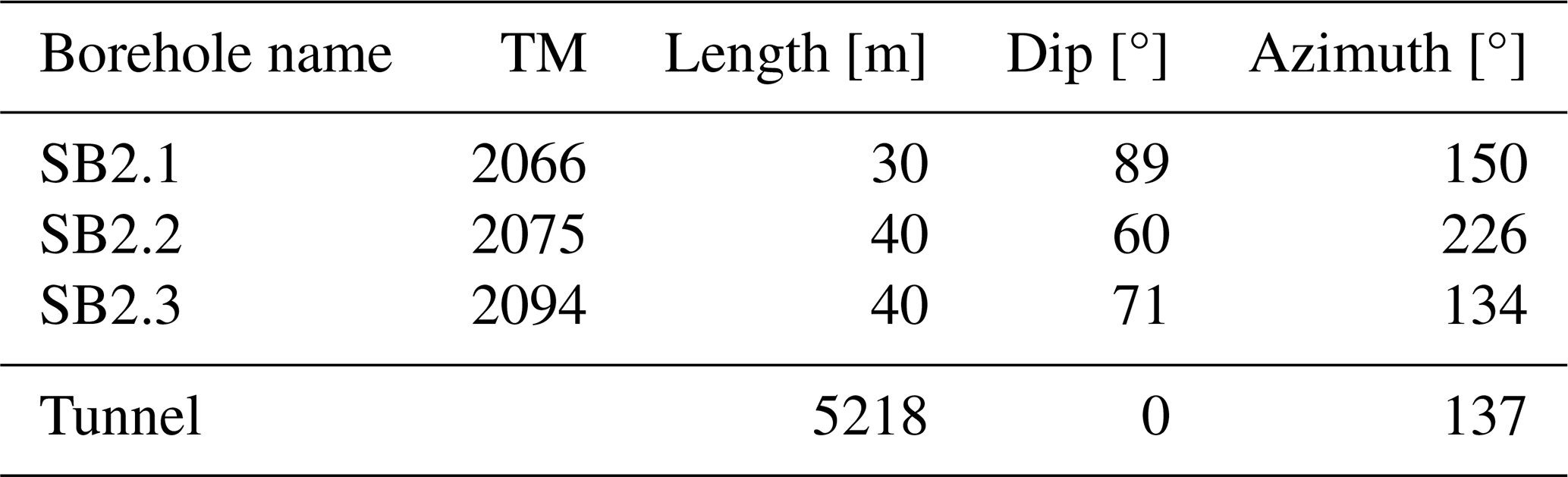
The Bedretto Lab hosts several boreholes of different lengths, partly equipped with permanently installed sensors. An overview of the lab and the boreholes is shown in Fig. 1. For this study, the boreholes SB2.1, SB2.2, and SB2.3 were used for extensive active seismic surveys. These boreholes are also called “tripod boreholes”, as they are pointing downwards in three different directions, spanning a tripod. The penetrated and analyzed Rotondo granite does not show any major fault or fracture zones close to the tripod, so we can assume that the rock volume is homogeneous. The boreholes were originally drilled for stress measurements of the background rock, so the stress conditions around the boreholes and the Bedretto Lab in general are well known (Bröker et al., 2024; Bröker and Ma, 2022).

The boreholes are located at the end of the lab niche, at TM 2066 to TM 2094, measured from the southern entrance of the tunnel. The vertical and inclined boreholes are assumed to be straight, with a length of 30 and 40 m, respectively, and a diameter of 101 mm. They are completely water-filled and freely accessible, which allows the usage of different seismic sources and receivers, explained in Sect. 4. Detailed information on the borehole orientations is given in Table 1.

The borehole trajectories used for the following analyses are based on a combination of wireline logging (with televiewer and other downhole tools) and laser measurements. Laser measurements allow a highly precise measurement of single points in the boreholes, used to interpolate the trajectories in between. In the lower part of the boreholes, laser measurements were not feasible anymore, as the water in the boreholes could not be pumped out completely. Instead, information on the azimuth and dip from several logging runs in the boreholes was used to determine the trajectory of the boreholes in the lower part. The combination of these two data sets allows a highly precise description of the borehole trajectories, which is crucial for anisotropy measurements.

4 Measurements

In the boreholes SB2.1, SB2.2, and SB2.3, introduced in Sect. 3, several different seismic cross-hole surveys were performed. The boreholes span one straight and two curved planes, allowing the measurement of the wave propagation in several different directions. The location in the tunnel and the orientation of the boreholes are also shown in Fig. 1.

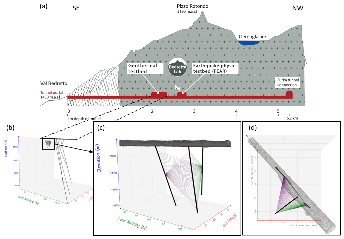
Figure 1 The used boreholes SB2.1, SB2.2, and SB2.3 are located in the Bedretto tunnel around TM 2000. A cross section of the tunnel, adapted from Keller and Schneider (1982), is shown in panel (a). The boreholes were used for extensive cross-hole seismic surveys involving various sources and receivers. The tripod and surrounding boreholes in the geothermal test bed are depicted in panel (b). Magnified views of the tripod are provided from the side and the top in panel (c) and (d), respectively. Exemplary rays in the three covered planes are represented by purple, gray, and green lines.

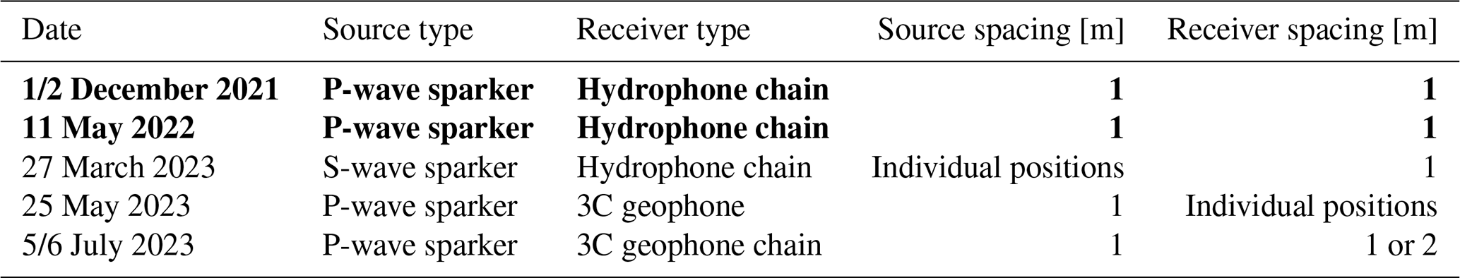
Table 2 Overview of the different measurement campaigns. The measurements used for this study are written in bold.

Results of the last campaign are shown in Appendix A.

The measurements were performed in different campaigns from December 2021 to July 2023. An overview of the measurements is given in Table 2. We started with a standard survey, using a P-wave sparker as a source and a hydrophone chain as receivers. The P-wave sparker used here is a monopole source discharging energy through two adjacent electrodes in a water-filled borehole. This energy discharge generates a pressure pulse, which initially spreads isotropically in the water and therefore also excites the borehole wall isotropically (Ellis and Singer, 2007). This creates a highly repeatable, high-frequency seismic signal propagating through the rock volume (, ).

All recordings were sampled with the highest possible sampling frequency of 48 kHz to record as much information as possible. The hydrophones, attached to a chain with 1 m spacing, can record pressure signals acting on the sensor from any direction, but the recorded data do not contain information about the incident angle of the seismic signal.

The recorded data of the first two surveys (December 2021 and May 2022) do not only show the arrival of P waves but also that of S waves. This can be explained by a P–S-wave conversion at the borehole wall near the source. The S waves traveling through the rock are back-converted in longitudinal waves when they hit the water of the receiver borehole, acting as a pressure impulse on the hydrophones.

In a next step, we determined the travel time of the different S waves in more detail. We accomplished this by employing a S-wave sparker as source, which emits a horizontally polarized, directed S wave. The data recorded in this survey have a high noise level and do not show the desired signals of S waves in the recordings, so we did not further consider the S-wave sparker data.

Instead we proceeded to record the signal of the P-wave sparker on three-component (3C) geophones. The geophones were clamped to the borehole wall, which allowed recording both the P and S waves directly on the rock surface on three mutually perpendicular components. Unfortunately, we were not able to determine the orientation of the sensor in the borehole, so neither a statement about the incident direction of the arriving waves nor an alignment of the sensors towards the source position can be made.

After some successful test measurements, we covered most of the test volume with 1 m spacing of both sources and receivers. Only in the uppermost and lowermost sections of the boreholes was the spacing between the receivers increased to 2 m due to logistical constraints, as it was not feasible to maintain the standard spacing in these regions. The aim of this survey was to further separate the differently polarized S waves from each other. During the data acquisition, we had to face several challenges, such as problems with the triggering of the recordings, the alignment of the sensors in the borehole, and a higher overall noise level, so this data set was only used as a comparison to the hydrophone recordings and to verify the arrival time of the S waves quantitatively. The data analyzed in the following include the recordings of the first two surveys, using a P-wave sparker as source and the hydrophone chain as a receiver.

5 Data analysis

The wave propagation of a seismic wave is controlled by the properties of the rock it is propagating through. Analyzing the travel time of the wave from the source to a receiver is a simple way to extract information about these properties. In the following, the recorded data from the first two surveys (December 2021 and May 2022) are presented and analyzed to characterize the undisturbed Rotondo granite in the Bedretto Lab.

The amplitudes of the P waves and most of the S waves are clearly visible in the raw data due to the short distances between source and receiver and a very low noise level in the test volume. The quality of the data was further increased by stacking three shots per position. No frequency filtering was applied. An exemplary receiver gather is shown in Fig. 2 (left) with single waveforms recorded on the hydrophones for selected traces (right). The receiver gather shows the signal recorded on a hydrophone in SB2.2 at 23 m depth for shot positions in SB2.3 from 3 to 38 m. The waveforms on the right correspond to the marked traces in the gather at shot positions of 9, 25, and 32 m depth. The same geometrical setup with recordings on the 3C geophones is shown in Fig. A1.

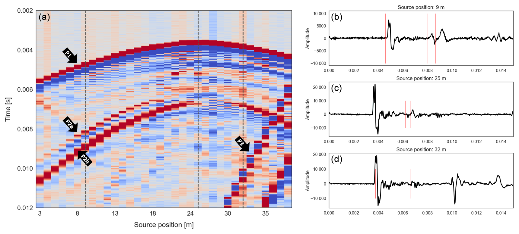
Figure 2 (a) An exemplary receiver gather for shot positions in SB2.3 with 1 m spacing recorded on a hydrophone in SB2.2 at 23 m depth. The onset of the P wave is clearly visible on all traces (P1). In the left part of the gathering, the splitting of the S wave in a fast (P2a) and slow (P2b) S wave is apparent. For shorter distances between source and receiver, the S wave gets covered in the coda of the P wave, and the splitting is not visible anymore. In some parts of the signal, other wave types, such as reflected or tube waves, are visible (P3), and they are not analyzed further. (b, c, d) The waveforms show the marked traces (dashed vertical lines) of the receiver gather. The red lines represent the expected arrival times. On all three traces, the arrival of the P wave is clearly visible. On the first trace, the S waves separate and can be picked. On the second and third trace, the arrival of the different S waves is less clear and cannot be picked accurately.

The onset of the P wave can clearly be identified for all shot positions (P1). The arrival of the S waves is only visible for longer ray paths (here source position 3 to 20 and 32 to 38, P2), where it is not covered in the coda of the P wave or by reflected waves, as is often the case for deeper shot positions. For some source–receiver orientations, a splitting of the S wave in a faster wave S1 (P2a) and a slower wave S2 (P2b) can be identified. This is a feature that can only occur in anisotropic media and is already a clear indicator that the granitic host rock is seismically anisotropic. A separation of different S waves is mainly identified in the plane between borehole SB2.2 and SB2.3, while only one S wave can be detected in the other two planes for most source–receiver pairs. In Fig. A2, more examples for different source–receiver geometries are shown for comparison.

The receiver gather in Fig. 2 also shows other wave types, such as reflected waves or tube waves, for deeper shot positions (P3). These signals are not considered in this study, as only the arrival time of the direct waves will be analyzed.

In the next step, the travel times for all unambiguous onsets were picked individually by hand and converted into apparent velocities, thereby assuming straight rays, which was judged to be a valid assumption in the relatively homogeneous host rock. The positions of sources and receivers are derived from the borehole trajectories, based on the known depth of the sensors along the borehole.

The apparent velocities (referred to as ray velocities in the following) must be evaluated with respect to their propagation direction to obtain information on the anisotropy of a medium. In Fig. 3, all source–receiver combinations are plotted as dots in a stereonet representation, colorized based on the velocity along the ray. We follow the geological convention of an azimuth of 0° pointing towards magnetic north, increasing clockwise, and a dip of 0° being horizontal, increasing downwards. The stereonet plots show the lower hemisphere representation.

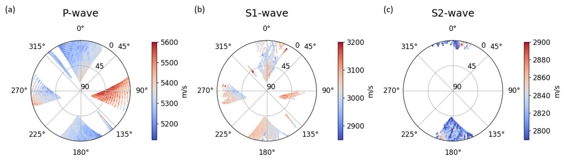
Figure 3 The stereonets show the apparent velocities of the three wave types, calculated based on the sensor positions and picked onset times. Each dot represents one source–receiver couple, colorized by the apparent velocity of the (a) P wave, (b) S1 wave, and (c) S2 wave. The number of picks decreases as S waves cannot be picked precisely on all data sets.

The stereonet plots show the angular coverage in the volume that we obtained from our sensor positions, as well as the number of picks we can determine for the different wave types. With our borehole orientation, we can cover mainly rays with N–S or E–W orientation for most dip directions. Only vertical rays (θ=90°) and rays in NE–SW and NW–SE orientations cannot be covered in our surveys, so we have no information on the velocities in these directions.

Looking at the color pattern in Fig. 3, a clear trend of faster and slower velocities is recognized for both P and S1 waves. Waves with E–W orientation travel faster than waves perpendicular to it with N–S orientation. The maximum of the P-wave velocity can be found in the right triangle, corresponding to rays in the plane between SB2.1 and SB2.2. Likewise, a trend of increasing velocities in a clockwise direction can be found for rays in plane SB2.2 to SB2.3 (upper and lower triangle), with minimum velocities in NNW–SSE orientation, perpendicular to the maximum velocity direction. While this trend is quite strong for P waves, a similar but less dominant trend can also be observed for S1 waves.

In the velocity pattern of the S2 waves, no clear trend of a velocity change is visible. However, only for certain ray directions can a splitting of S waves be detected. Different types of S waves can only be detected in the N–S direction, while the S waves are not clearly separated in the E–W direction. In general, the number of clearly identifiable arrivals decreases from P over S1 to S2 waves.

As mentioned in Sect. 4, the 3C geophone data were used to verify the recordings on the hydrophones. The arrival times of P and S1 waves were also picked on the 3C geophones and plotted in a stereonet plot. The result is shown in Fig. A3. The velocity pattern matches the pattern of the hydrophone data in Fig. 3, but the data quality is lower, so fewer picks are available and higher uncertainties are expected.

Based on the variation of the measured data, the anisotropy factor can directly be calculated by $(v^{\max }-v^{\min })/v^{\mathrm{mean}}$. It is describing the variation of the velocities, indicating how much they differ with respect to the propagation directions. Instead of using the maximum and minimum velocities, we used the average of the highest and lowest 5 % of the data to avoid a distortion of the result by outliers. For the P waves an anisotropy of 6.4 % is determined, and S1 waves show an anisotropy of 5.1 %. However, for both wave types, the real value might be even higher, as not all ray directions can be measured, and the maximum or minimum velocities might be missed.

We are aware that also uncertainties in the borehole trajectories and thus in the source and receiver positions can mimic anisotropy in an intrinsically isotropic rock (Maurer and Green, 1997). The fact that we can detect shear-wave splitting for some ray directions, as well as the highly precise measurements of the borehole trajectories, precludes the option of wrongly assuming anisotropy in our rock volume.

6 Results

In Sect. 5, we already mentioned that the picked travel times of the measured seismic signals show the expected velocity pattern of a TTI medium. Now we explain the measured data with an anisotropic velocity model defined by the Thomsen parameters to identify the potential sources causing the seismic anisotropy. Also, the sensitivities of the model parameters need to be analyzed to understand the reliability of the model.

In a first step, a grid search over the whole parameter space for ϕ₀ and θ₀ and the relevant parameter values for ϵ and δ was used to determine a set of parameters describing the P-wave data. After the first run, a second grid search with refined grid spacing close to the best fitting parameters was performed. The value of α₀=5115 m s⁻¹ was kept fixed for both runs, based on values from previous measurements (Schneider, 2022).

Table 3 The table shows both the parameter range of the grid searches ([start value, end value, step size]) and initial values of the optimization as well as the optimized parameter sets after (a) the general grid search over the whole parameter space, (b) the refined grid search around the optimum of (a), and (c) the optimization algorithm. The last column shows the root-mean-square error of the P waves for the grid search and the weighted root-mean-square error of all wave types for the optimization algorithm. All values are in the respective units.

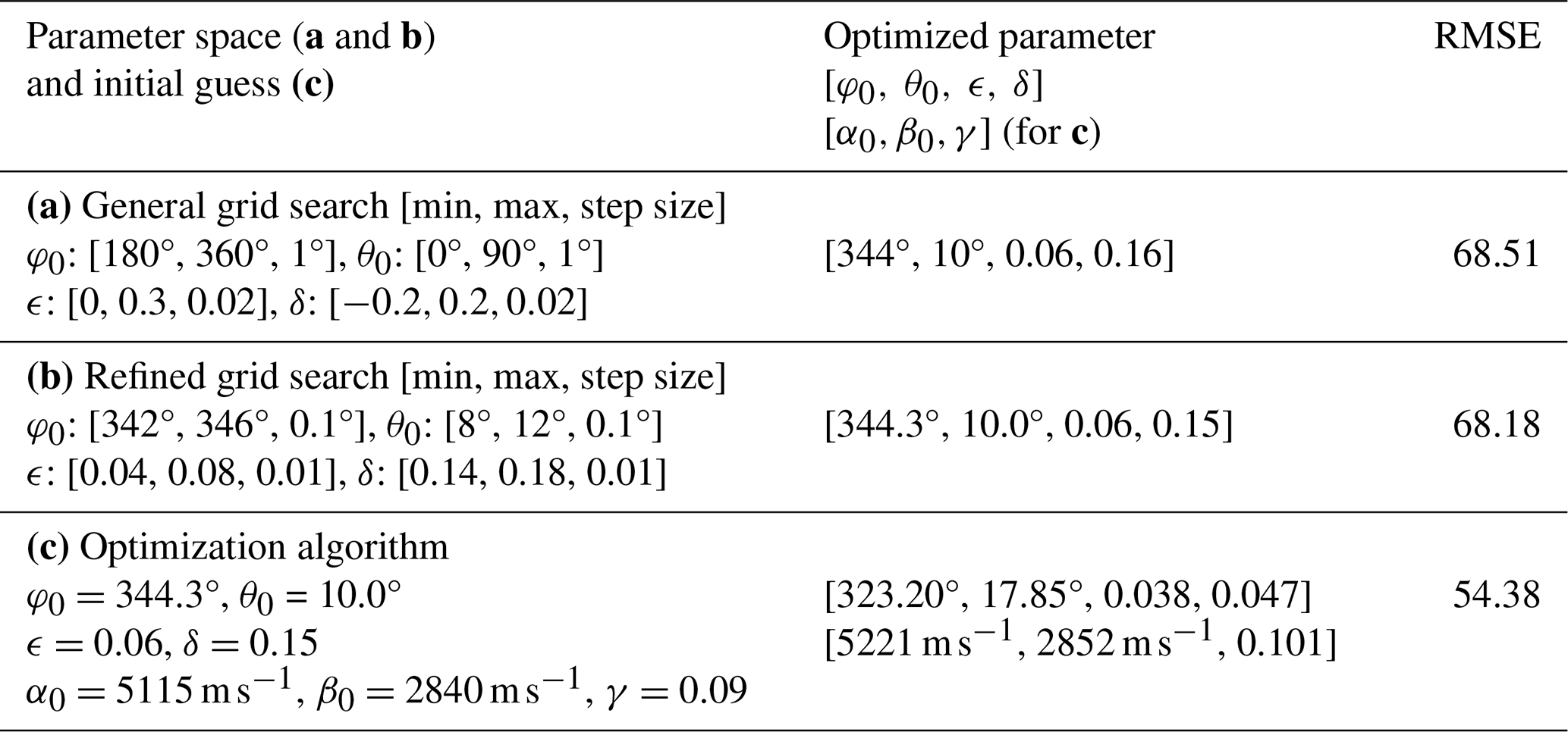
The refined grid search results were further improved by a downhill simplex algorithm, minimizing the root-mean-square error (RMSE) between the modeled and measured velocities of all three wave types. Here we assume that the faster S wave in our data (P2a in Fig. 2) is horizontally polarized (with respect to the elastic tensor orientation) and can be described by Eq. (2). We will justify this assumption in Sect. 6.2 based on the picked data. The RMSE of the different wave types was weighted to take the uncertainty of the different S waves into account. The RMSE of the P waves was weighted higher with a value of 0.6, while S1 and S2 waves are weighted by 0.3 and 0.1, respectively. The parameter space and results of the grid search and optimization algorithm are summarized in Table 3.

The optimized parameters indicate an inequality of ϵ<δ. While many studies report the opposite ratio, with ϵ>δ, there are also examples consistent with our findings (e.g., Thomsen, 1986, or Horne, 2013). It is important to consider that many investigations of anisotropy focus on sedimentary rocks, which are only partially comparable to the igneous rock type examined in our study. Research on more comparable igneous rocks has also concluded that ϵ⩽δ is a realistic scenario (Boese et al., 2022; Doetsch et al., 2020; Motra et al., 2018). However, the absolute values of the Thomsen parameters vary significantly with pressure, temperature, and mineral composition, making direct comparisons between studies challenging.

Additionally to the model fitting, a sensitivity analysis was carried out to investigate the reliability of the optimized parameters. This is particularly important for the deeper understanding and interpretation of the optimized model. The model resolution matrix of all three wave types individually, as well as a matrix combining all three wave types, is analyzed to highlight the importance of combining information from all three wave types to fully describe the elastic tensor of the rock.

6.1 Sensitivity analysis

The results of the sensitivity analysis are shown in Fig. 4 for the analysis of the single wave types (a–c) and the combination of all wave types (d). In the matrix itself, the values and the colors are normalized by the diagonal element of each row to show the trade-off between the different parameters. The column on the left represents the absolute values of the diagonal entries of the matrix for each parameter to show how well each parameter can be resolved based on our setting. White diagonal elements mean that the wave type does not provide any information on this parameters. White colors on the off-diagonal mean that there is (almost) no trade-off between the parameters (normalized values between −0.05 and +0.05 are also plotted in white to simplify the matrix).

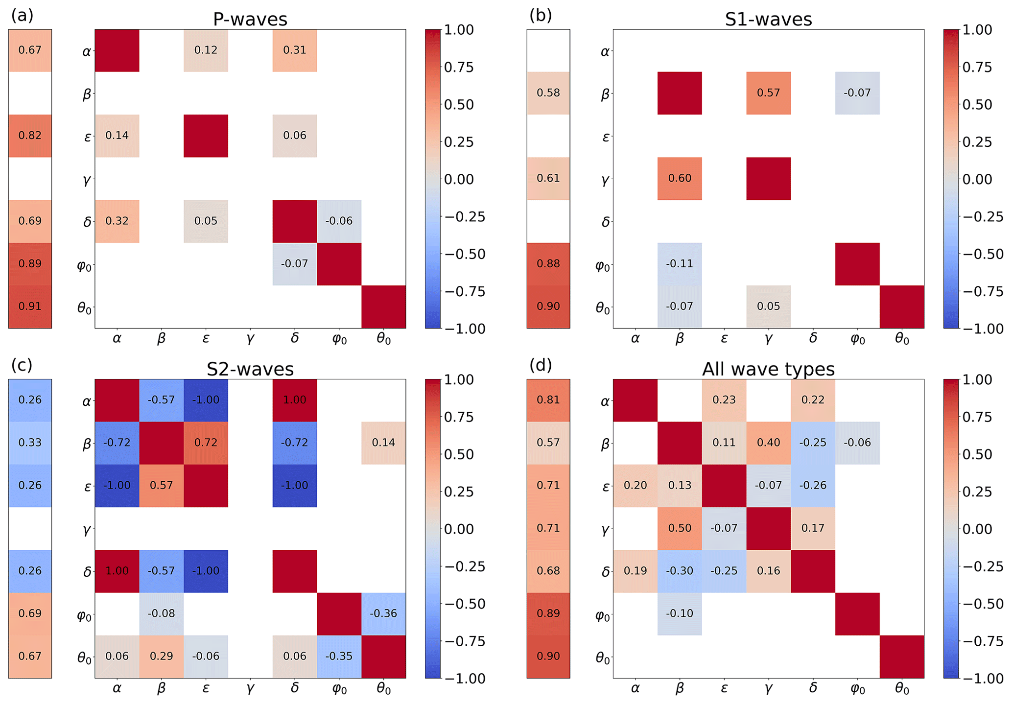
Figure 4 The model resolution matrices, using only one wave type (a, P waves; b, S1 waves; c, S2 waves) and combining the information of all three wave types (d). The column on the left shows the relative difference of the diagonal elements, while the values in the matrix are normalized for each row by the diagonal element.

Matrices (Fig. 4a–c) directly show that none of the wave types can provide information on all seven parameters describing the elastic properties of the rock volume. While all wave types provide information on the orientation of the symmetry axis (φ₀ and θ₀), each wave type contains only information about a subset of the Thomsen parameters. The matrices further show that the orientation of the symmetry axis is highly constrained, even if only one wave type is used in the analysis. This is expected, as we can cover many different ray directions with our borehole orientation.

If only P-wave data are used to model the anisotropy, information on β and γ is completely missed. Combining the information of P waves with the travel times of S1 waves can close this gap and fully describe all parameters, as the different waves contain complementary information. The S1 wave is not controlled by δ, so the trade-off between φ₀ and δ, which is present for P waves, can also be eliminated by adding the S1-wave data to the model.

The absolute velocities of the waves along the axis, represented by α and β, are affected by the parameters ϵ, δ, and γ for P and S1 waves. Figure 4a also shows a trade-off between ϵ and δ; however, this trade-off is negligibly small. The small trade-offs between the different parameters are also apparent in the diagonal element values shown in the left column. Both angles have a value of about 0.9, showing that they are highly constrained by our data. The other parameters of both P and S1 waves are mostly larger than 0.6, indicating that these parameters are also acceptable but still less constrained. Only β is slightly lower for S1 waves, as a stronger trade-off with γ is present.

The matrix of the S2 waves (Fig. 4c) shows a different behavior. S2 waves contain information on almost all parameters; only γ is not controlling the S2-wave velocity.

As before, the orientation of the symmetry axis has the highest absolute values and indicates the least correlation to other parameters. However, the Thomsen parameters show a very high trade-off between each other. Especially the contrary influence of δ and ϵ on α leads to inconclusive information on these parameters, as errors in one parameter might be compensated by the other parameter. The different parameters cannot be resolved independently, resulting in very low constrained absolute values for all Thomsen parameters, including the velocities α and β. Nevertheless, information of the S2-wave velocity should be included in the final model to avoid artificially constraining the final model.

In Fig. 4d, the model resolution matrix R for the combined analysis of all three wave types is shown. Combining the information of all wave types results in a highly constrained model for all seven unknowns of a TTI model. The orientation of the symmetry axis has, as for all single-wave information, no significant trade-off with any other parameters. Most of the other parameters show a small trade-off between each other, with absolute values smaller than or equal to 0.3, except from β to γ. The high diagonal elements for all parameters indicate that we can have a high confidence in the accuracy of the optimized parameters.

The higher trade-off between β and γ results from the fact that γ is only controlling the wave propagation of the S1 wave, so the other wave types cannot compensate for this trade-off, as is the case for other parameter combinations. More measurement points of the S1 waves could help to improve this correlation; however, the S1 wave is partly covered by the coda of the P wave or tube and reflection waves, which makes an accurate determination of the travel time in some directions impossible.

6.2 Analysis of the model fit

The result of the optimized model in comparison with the measured data is shown in Fig. 5. The background color shows the velocity distribution based on the optimized parameters from Table 3c, while the dots in the foreground show the actually measured data. The color range for both the measured and optimized data is the same, so measurement points that are hard to distinguish from the background represent a high accordance with the optimized model.

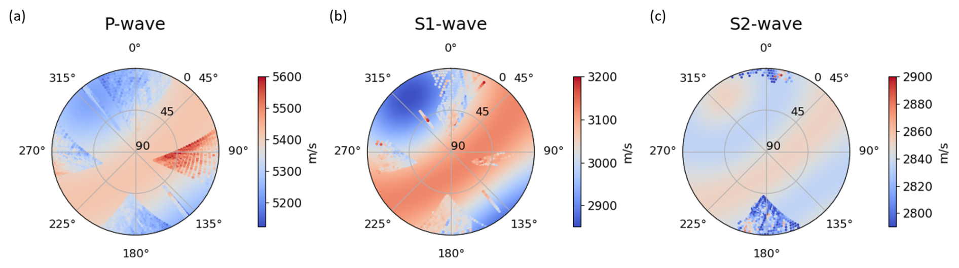
Figure 5 The background color shows the apparent velocities for the (a) P wave, (b) S1 wave, and (c) S2 wave based on the optimized TTI model. Dots in the foreground represent the measured apparent velocities for the covered ray directions.

The optimized model fits the pattern of the measured data of the P and S1 waves quite well. This further confirms our assumption of a TTI medium. While the maximum magnitude of the P waves is slightly underestimated, the magnitude of the S1 wave is in good accordance with the optimized model. Especially the trend of increasing velocities away from the symmetry axis at φ₀=323.20°, θ₀=17.85° towards the symmetry plane perpendicular to it, mainly visible in the upper and right triangle, fits very well to the measured velocities. S2 waves can only be picked in the plane between borehole SB2.2 and SB2.3. In this plane, less interference with other wave types is disturbing the signal, and the travel time difference between the S1 and S2 waves is large enough to separate the different waves. The measured S2-wave velocities do not show a strong velocity change with the ray direction but only small amplitude variations from 2800 up to 2900 m s⁻¹.

While Fig. 5 shows the measured data with respect to the ray orientation in the rock volume, Fig. 6 shows the same data but for the ray orientation with respect to the elastic tensor orientation. The apparent velocities of all three wave types are plotted against the angle ξ, clearly showing the increasing velocities of P and S1 waves for increasing angles ξ. The S2 waves show only a poor variation in the velocity with the ray direction. The black lines represent the expected velocities based on the optimized TTI model, following the same trend as the real data. This shows that the model can explain the stronger variations of P- and S1-wave velocities and the poor variation of the S2-wave velocities at the same time.

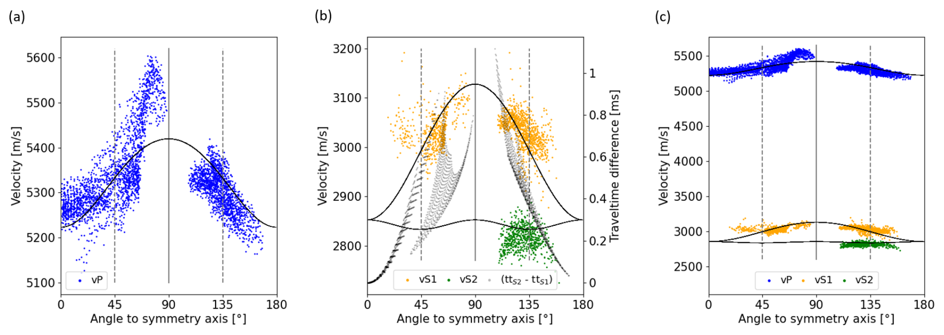
Figure 6 The measured velocities of (a) P waves, (b) S waves, and (c) all wave types plotted against the angle ξ between the straight ray and the optimized symmetry axis. The black line represents the expected velocities based on the optimized model parameters. The vertical lines represent angles of 45° and 90° (symmetry plane) as well as 135° to the symmetry axis.

This plot does not only show the good data fit but also verifies our assumption of the permanently faster S1 wave. In Fig. 6b the velocities of the faster S wave are plotted in yellow, and the velocities of the slower S wave are plotted in green. The different point clouds show clearly distinguishable velocities, which rules out the option that not one of the waves is permanently faster but that the order of the wave type arrival changes with different ray directions. Furthermore, the trend in the velocity of the S1 wave is constantly increasing up to its maximum in the symmetry plane (at ξ=90°), which indicates that the faster wave is a horizontally polarized wave, described by Eq. (2).

Additionally to the picked and expected apparent velocities, Fig. 6b also shows the expected differences in the travel time of the S1 and S2 waves in black. As already mentioned, the S waves only split up in certain directions if the velocity difference is large enough and the traveled distance is long enough. Indeed, we can pick the slower S wave mainly in ray directions, where the expected travel time difference is maximized (for angles around 120°).

Not only the travel time difference itself but also the overall data quality is important to pick the second S wave. While the data quality is rather high for rays with angles >90°, the quality is either lower or parts of the signal are covered in reflection or tube waves for angles <90°, so the picking of the slower S wave cannot be done for these rays. This explains why no S2-wave picks are available for these angles even though the expected travel time difference is similarly high.

Analogous to the anisotropy factor based on the measured data, the anisotropy factor can also be calculated for the model data. The P waves show an anisotropy of 3.5 % in the optimized model, and the S1 waves show an anisotropy of 6.6 %. These values are in the same order of magnitude as the anisotropy factors of the measured data in Sect. 5.

The optimized TTI model can explain the measured data to a first order, but it still shows a systematic misfit, shown in Fig. 7. The representation is the same as before, but the color refers to the absolute misfit for each ray direction. The maximum, absolute misfit of all wave types is in the range of about 200 m s⁻¹, which corresponds to an offset of about 3 %–7 %. This shows that the final anisotropic velocity model explains the measured data reasonably.

The misfit shows trends of over- and underestimated velocities for P and S1 waves. For P waves, velocities in E–W directions are mainly underestimated, while rays with N–S orientation are overestimated by the model. The error of the S1 waves shows a less dominant pattern but is still not randomly distributed and shows underestimated velocities for mainly horizontal rays and rays in the NW–SE direction such as overestimated velocities for steeper ray directions. The model overestimates the S2-wave velocities for most ray directions. It is also remarkable that the shear-wave splitting is mainly detected in parts where the P-wave velocity is overestimated, while the S1-wave velocity is underestimated. A model with a higher fit in these parts could potentially result in a higher expected travel time difference than assumed by our model, fitting to a splitting in these parts.

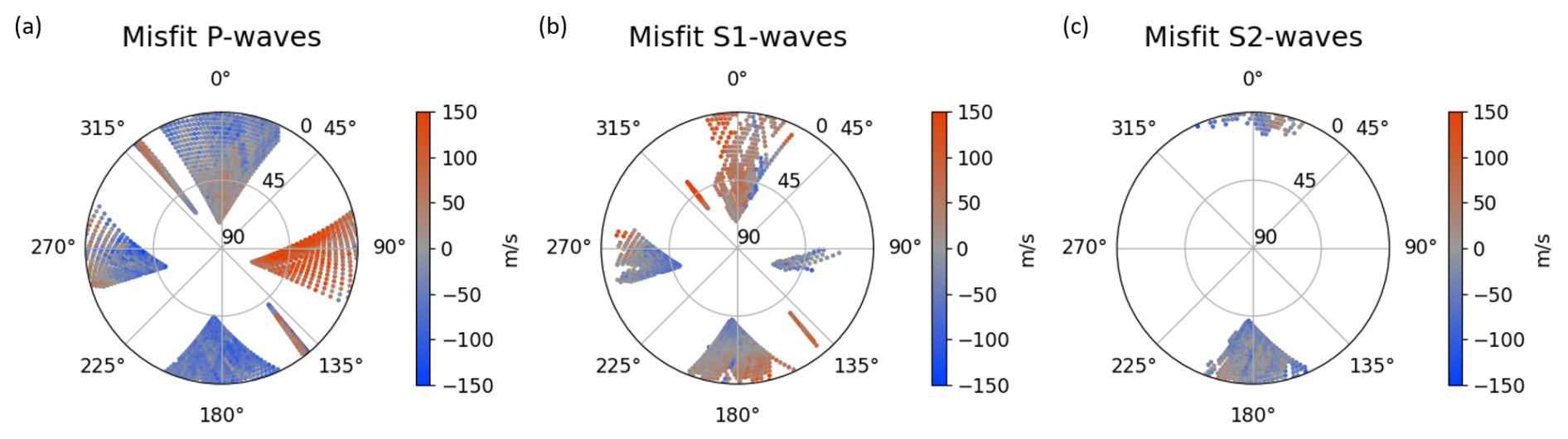
Figure 7 The stereonets show the misfit between the optimized model and the measured apparent velocity for all picked data. The range of the color bar is equalized and clipped for a better comparison of the misfits and to avoid distortion by single outliers. A negative misfit means that the optimized model is overestimating the velocity.

While such a systematic error is an indicator of an inadequate assumption in the model, the overall fit of our model is still adequate, and it can be used for further characterizations of the rock volume. Potential sources for the observed anisotropy are discussed in the following Sect. 7 by comparing our results to other studies.

7 Discussion

The picked travel times of the P waves give evidence for seismic anisotropy in the volume of interest, which can by first order be described as a TTI model. This symmetry is further confirmed by the two different shear waves following matching patterns. The high angular coverage in the tripod boreholes, as well as the large number of picked arrival times for all three wave types, allowed us to determine a well-constrained anisotropic velocity model.

While it is common to analyze the seismic anisotropy of a rock on the lab scale (David et al., 2020; Schneider, 2022; Sayers, 2002; Nur and Simmons, 1969) and for rock types other than igneous rocks (Al-Harthi, 1998; Chan and Schmitt, 2015; Song et al., 2004), it is often not taken into account on the field scale for igneous rocks. This cannot only lead to flawed results in the velocity model, but also important information on the rock characteristics is neglected.

The analysis of seismic anisotropy on the field scale offers significant advantages over lab-scale experiments. While measurements in the laboratory give only insights on the features of the undisturbed rock, fractured or brittle material can also be tested on the field scale. It is known that open and filled fractures are crossing the volume of interest, potentially influencing the wave propagation in our test bed. These effects are missed in lab-scale experiments.

Another advantage is the interpretation of the result in a larger context. The laboratory can only offer quantitative information about the elastic tensor but not about the orientation of it in the field. However, the orientation of the tensor, described by the symmetry axis, is of high importance to identify the causative factors of anisotropy. Not only the orientation of the sample but also the in situ conditions cannot be preserved in the laboratory. During the exhumation of the rock, a non-reversible relaxation of the sample occurs, altering the external forces that control its elastic properties.

In the following, we consider various factors that may control anisotropy, and we discuss how adequately they can describe our measured anisotropy. Different factors are known to cause seismic anisotropy on different scales (Barton, 2006):

• interbedding of sedimentary rocks,

• fault zones,

• fabrics,

• natural fractures, and

• stress field orientation.

The first two factors can be eliminated in our rock volume, as the tripod is placed in an undisturbed part of the Rotondo granite. Different logging runs proved that the boreholes are not crossing any major fault zones or larger fracture zones. The seismic data also have no indication for larger heterogeneities within the test volume, which is in good accordance with the geological characterization of Jordan (2019). The fabrics of the rock can also be excluded as a potential source, as the thin sections and core samples of the undisturbed granite do not show any preferred orientation or mineral alignment (David et al., 2020; Ma et al., 2022; Jordan, 2019). The undeformed Rotondo granite is also fully isotropic under high pressures in the lab, indicating that the anisotropy is not intrinsic from the material itself but must be controlled by external factors (Schneider, 2022). Under high pressure, all cavities are closed, so a preferred orientation of the minerals would cause anisotropic velocities.

The remaining factors that are known to cause anisotropy are (natural) fractures and the predominant stress field in the rock volume. The occurrence and orientation of the fractures in the tripod boreholes are analyzed in Bröker et al. (2024). Jordan (2019) additionally mapped fractures along the tunnel wall. We use a combination of both studies to describe the fracture network around the tripod. This ensures that we do not underestimate the fracture density in a specific direction (sub-)parallel to the boreholes (Terzaghi, 1965). A detailed analysis of the undersampled fractures for each borehole and the tunnel is shown in Fig. A5.

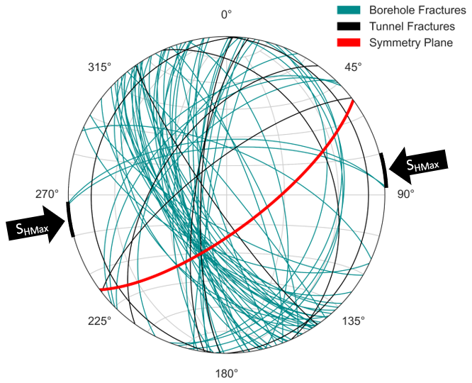
Figure 8 The stereonet represents the natural fractures along the tunnel wall from TM 2050–2115 (black) and in the boreholes (turquoise) and the symmetry plane (red) of the optimized anisotropy model. The black arrows point towards S_HMax around the tripod boreholes as estimated from mini-frac tests by Bröker et al. (2024).

The mapped fractures of both studies are summarized in Fig. 8. Black lines represent the strike direction of mapped fractures along the tunnel, and turquoise lines represent the strike direction of the mapped fractures of the logging data. The fractures mapped in the tunnel show a slight trend of N–S-striking fractures around the tripod boreholes, which is supplemented by NW–SE-striking fractures in the logging data. In both data sets, the fractures are mainly sub-vertical. The fractures mapped in the borehole are mainly dipping towards the east or southeast, the fractures mapped along the tunnel wall do not show a dominant dip direction.

However, in addition to the fractures, stress-induced anisotropy is also a possible source for the measured anisotropy in the tripod. The magnitude and orientation of the stress field around the tripod is analyzed by Bröker and Ma (2022) and Bröker et al. (2024), respectively. They state that one of the principal stress components is vertically oriented (S_V) and in the same order of magnitude as the maximum horizontal stress (S_HMax), pointing in the N75° E to N87° E direction around the tripod boreholes. The orientation of S_HMax, estimated from mini-frac tests, is also plotted in Fig. 8 by the black arrows.

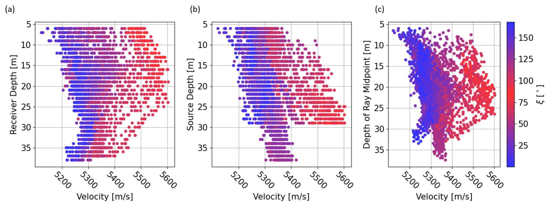
Figure 9 The figure plots the measured P-wave velocity against the depth of (a) the source, (b) the receiver, and (c) the midpoint of the ray. The color bar shows, in contrast to the measurement depth, the angle between the ray and the symmetry axis of the TTI model. Blue colors corresponds to rays that are (sub-)parallel to the symmetry axis, and red colors corresponds to rays that are (sub-)parallel to the symmetry plane.

Also, the variation of the stress field with increasing depth should be taken into account. The vertical stress component is assumed to increase with increasing depth as the overburden increases by about 3 % along the tripod boreholes. However, horizontal stress component variations do not correlate with increasing depth, as they are mainly controlled by other factors such as the proximity to fractures (Bröker and Ma, 2022). The depth effect on the P-wave velocity is illuminated in Fig. 9. It shows both the effect of the measurement depths and the effect of the ray direction on the velocity. This makes clear that the effect due to increasing source or receiver depths is much smaller than the effect due to the ray direction. Rays with a similar orientation, i.e., similar colors, show an increase of not more than 100 m s⁻¹ for increasing depth, while the velocity variation due to the ray direction is in the range of 400 m s⁻¹.

Comparing the orientation of the fractures and the in situ stress field with the orientation of the anisotropy can reveal information about the correlation between the different characteristics. In the case of a purely fracture-dominated anisotropy, we would assume faster velocities along the fractures and minimum wave velocities perpendicular to it (Barton, 2006). In the tripod, this would correspond to faster velocities in a vertical plane with N–S to NW–SE orientation and a symmetry axis in E–W to NE–SW direction. In the case of a purely stress-induced anisotropy, faster wave velocities are expected along the maximum principal stress direction (Nur and Simmons, 1969; Barton, 2006; Song et al., 2004). This means that in the case of S_V ≈S_HMax, the seismic velocities are not just maximized in one specific direction but within the plane spanned by the two maximum stress directions. In the case of the tripod, this plane is oriented in an E–W to NE–SW direction.

In Fig. 8 the relations between the fracture network (lines in black and turquoise), the stress field (black arrows), and the symmetry plane of maximum velocities (red) are summarized. The symmetry plane with maximum velocities is rather aligned with the maximum stress directions than with the preferred orientation of fractures in the tripod. Also, the velocity pattern corresponding to a mostly rotationally symmetric TTI medium fits the expectation of a stress-induced anisotropy with S_V≈S_HMax.

However, the orientation of the symmetry plane cannot exclusively be explained by the stress field, which suggests that a combined effect of the fracture network and stress field is controlling the anisotropy in the tripod. Also, the systematic distribution of the misfit indicates that the assumption of a homogeneous TTI medium might be too strong and cannot fully cover our observations. The heterogeneous distribution of filled and unfilled fractures along the boreholes gives more complexity to the velocity field and potentially also reduces the symmetry from a hexagonal TTI medium towards a slightly orthorhombic medium.

Our measurements are not just in accordance with the orientation of the in situ stress field but also quantitatively with first lab measurements from David et al. (2020) and Wenning et al. (2018) on the Rotondo granite. They measure a seismic anisotropy of about 6 % under zero-confinement pressure and 30 MPa confinement pressure, respectively. However, in both studies only a limited number of ray directions were measured, so the maximum and minimum velocity direction might be missed, and the true anisotropy might also be higher.

A common explanation for seismic anisotropy on the lab scale is the preferred orientation of so-called microcracks in the sample, which is controlled by the applied stress field, closing cracks perpendicular to the maximum stress direction. This effect is not fully reversible, so the samples in the lab still behave anisotropically even without any applied differential pressure.

This explanation of the closure of microcracks might be true for sedimentary rocks with a significant amount of microcracks between the grains. However, microcracks are less dominant in igneous rocks, so this effect is assumed to be small (Howarth, 1987). Maitra and Al-Attar (2021) state that the effect of differential stress on a solid medium can rather be explained by a change in the elastic tensor of the effective medium than by the effect on its cavities. The elastic tensor is affected by the in situ stress field with three distinct principal stresses, causing a higher stiffness of the material along σ_max, increasing the wave velocity along it.

It is known that uncertainties in the borehole trajectory can cause a comparable velocity pattern, mimicking seismic anisotropy, or change the TTI model (Maurer and Green, 1997; Hellmann et al., 2023). The velocity pattern based on an earlier and less accurate trajectory calculation is shown in Fig. A4. It shows a similar but rotated velocity pattern with faster velocities in the NE–SW direction, rather than in the E–W direction. This further demonstrates that the anisotropy model is highly sensitive to errors in the borehole trajectories.

However, the occurrence of the splitting of the two differently polarized S waves is clear evidence for true seismic anisotropy in the volume of interest. Additionally, the trajectories of the boreholes used in this study are known with up to a millimeter precision. This allows the determination of a reliable final model that can be used for further analyses on the source of the anisotropy. The relation between borehole trajectories and seismic anisotropy calculations will be analyzed in more detail in an upcoming study.

8 Conclusions

The cross-hole seismic data set measured in the tripod boreholes of the Bedretto Lab allows a reliable determination of a TTI model. We were able to measure wave velocities in a large range of directions, covering most azimuth and dip directions. The detection of the different wave types (P, S1, and S2 waves) further constrains the velocity model as the wave velocities contain supplementary information of the elastic tensor. The most likely cause of the anisotropy is a combination of the stress field and the fracture network. The stress field can explain the main features of the velocity distributions, with a rotationally symmetric pattern around the symmetry axis pointing towards the minimum stress direction. However, deviations from this TTI model, which become particularly evident in the systematic misfit, can be assigned to the orientation of the fractures in the volume. A more complex model with a lower (orthorhombic) symmetry could potentially account for these effects, but the lack of data, especially within the symmetry plane, makes a reliable calculation of an orthorhombic medium impossible.

Appendix A

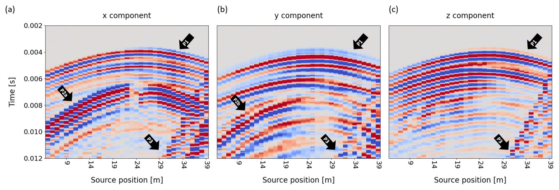
Figure A1 The receiver gather for the same geometry as in Fig. 2 recorded on a 3C geophone (receiver in SB2.2 at 23 m depth, source in SB2.3 with 1 m spacing). The P-wave arrival is clearly visible (P1). On the x component, the arrival of the S1 wave is visible (P2a); the onset recorded on the y component is slightly later and, thus, corresponds to the S2 wave (P2b). On the z component, no S-wave signal is recorded. All components also contain reflected or tube waves (P3).

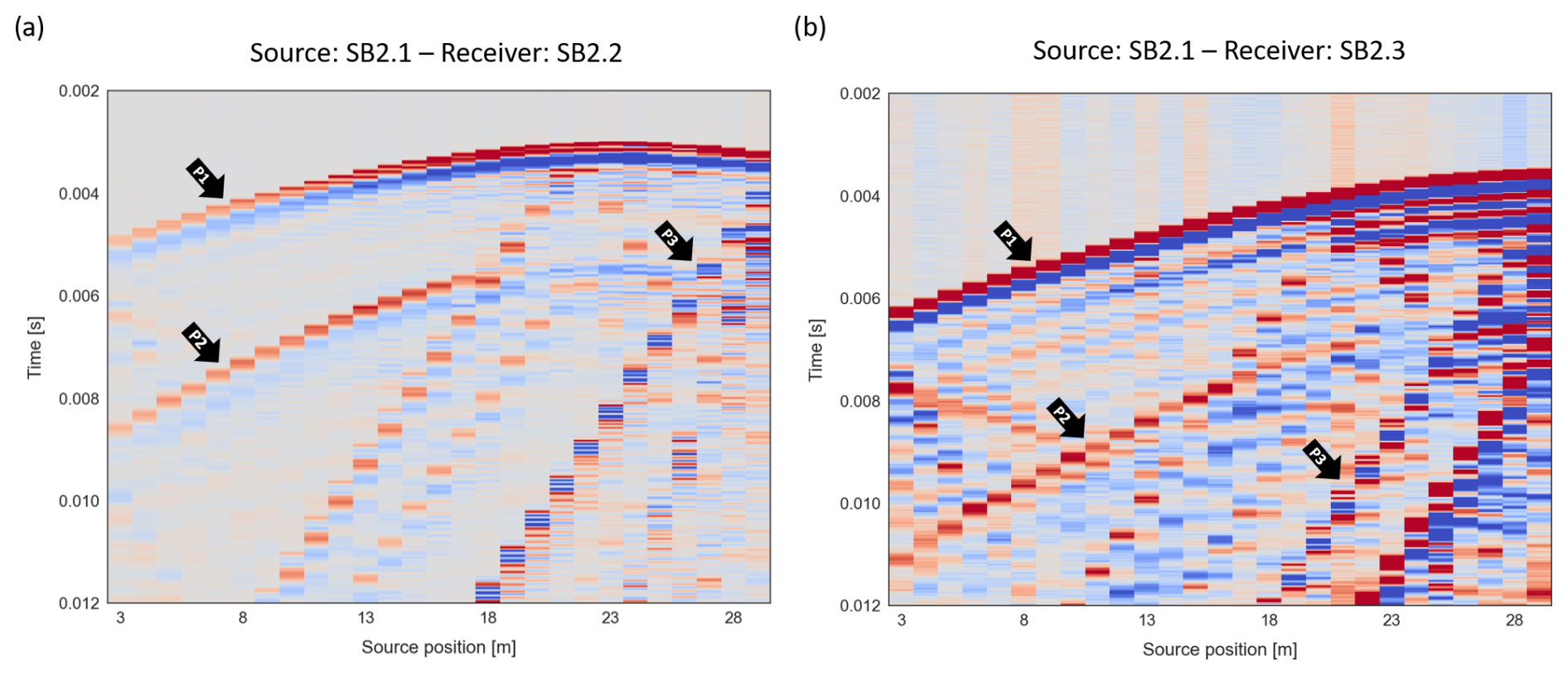
Figure A2 (a) Shot gather of a source in borehole SB2.1 at 26 m depth, recorded on hydrophones in SB2.2 with 1 m spacing. (b) Shot gather of a source in borehole SB2.1 at 32 m depth, recorded on hydrophones in SB2.3 with 1 m spacing. Arrows point to the P-wave arrival (P1), S1-wave arrival (P2), and reflected or tube waves (P3). In both geometries, no clear splitting of the S waves is detected.

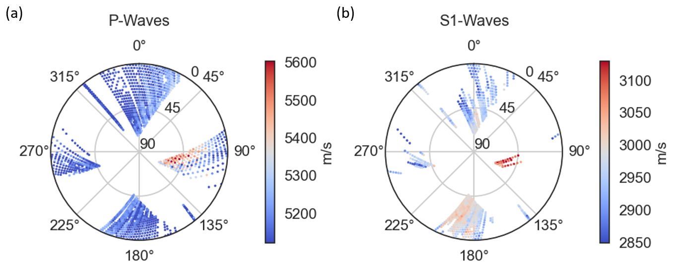
Figure A3 Calculated apparent velocities based on the picked travel times on the 3C geophones. The overall pattern fits the velocity pattern of the hydrophone data set, but the magnitudes are smaller compared to the hydrophone data set. Problems in the data acquisition, triggering the recording, can explain this shift.

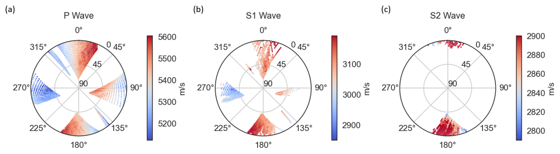
Figure A4 Apparent velocities for all three wave types, based on the old trajectories. These trajectories have a higher uncertainty as they are purely based on logging information.

Figure A5 The stereonet shows the directions of undersampled fractures for each borehole and the tunnel. The solid line represents the poles of fractures parallel to the borehole, and the dashed lines represents the poles of fractures with an angle of ±16° to the borehole and the tunnel direction, respectively. Palmström and Strömme (1996) state that fractures with an angle of up to 16° to the borehole are underrepresented in the data. The single dots show the orientation of the boreholes and tunnel itself. Fractures with pole orientations within the dashed lines of each borehole are expected to be undersampled by logging data of the corresponding borehole or tunnel.