Multiphysics property prediction from hyperspectral drill core data

Hyperspectral data provide rich information on both the mineralogical and fine-scale textural properties of rocks, which also control their petrophysical characteristics. We propose that some physical rock properties can be predicted directly from hyperspectral data, improving petrophysical characterisation and reducing the need for often laborious measurements. In this contribution we explore correlations between hyperspectral and petrophysical data using a deep convolutional neural network. Our model learns relevant features from high-dimensioned hyperspectral data to predict slowness, density, and gamma-ray values using training and testing data from Spremberg, Germany. Our results show that, with careful preprocessing and thorough data cleaning, differences in resolution can be overcome to learn the relationship between hyperspectral data and petrophysics. Using a test dataset from a spatially independent borehole, we generated a pixel-resolution (≈1 mm²) model of the petrophysical properties and resampled it to match the measured logs. This test indicated substantial accuracy, with R² scores and root-mean-squared errors (RMSEs) of 0.7 and 16.55 µs m⁻¹, 0.86 and 0.06 g cm⁻³, and 0.90 and 15.29 API for the slowness, density, and gamma-ray predictions respectively. We also analysed the Shapley values of our model to gain deeper insights into its predictions. These findings lay the groundwork for building deep learning models that predict physical and mechanical rock properties from hyperspectral data. Such models could provide the high-resolution but large-extent data needed to bridge the different scales of mechanical and petrophysical characterisation.

1 Introduction

Hyperspectral imaging provides detailed insights into the mineralogical composition of rocks by capturing minute spectral signatures across extensive wavelength ranges. This technology enables rapid, non-invasive characterisation and spatial analysis, with diverse applications for geological mapping, minerals exploration and geometallurgy. These applications typically leverage the unique combination of millimetre-scale spatial resolution and kilometre-scale extent possible with hyperspectral drill core or outcrop scanning methods (Thiele et al., 2021, 2024a; Laukamp et al., 2021).

Geophysical well logging has been employed to acquire petrophysical data from boreholes utilising a suite of tools to measure various properties in situ. This process includes the collection of gamma-ray, density, and sonic logs, which provide continuous and high-resolution records of the subsurface properties. Gamma-ray logs are often used to identify shale-rich layers by measuring the natural radioactivity of the formations, primarily from potassium, thorium, and uranium content (Serra, 1984). Density logs, which measure bulk density through the attenuation of gamma rays, can be used for the estimation of porosity and lithological differentiation (Schlumberger, 1972). Sonic logging is used to measure the travel times of acoustic waves travelling through the formations, providing insights into both the mechanical properties and porosity of the rock, through the measurement of slowness (inverse of P wave velocity) (Bourbié et al., 1987).

While hyperspectral data are primarily known for their sensitivity to mineralogy (Clark, 1999), they are theoretically also sensitive to textural attributes such as grain size, especially in the mid- and long-wave infrared regions. Initial work by Kereszturi et al. (2023) and Lee et al. (2023) has built on these theoretical connections to successfully predict petrophysical and geomechanical properties, albeit on relatively small sample sets. In this contribution, we build on this work to test if “hyperspectral upscaling” workflows that were developed to predict mineralogy (e.g. Thiele et al., 2024a) can also be used to map petrophysical properties along drill cores at high (millimetre-scale) spatial resolution. In doing so, we aim to both enhance the spatial resolution of downhole petrophysical logs and work towards potentially generalisable methods that could, one day, be used to predict important petrophysical and mechanical properties across large drill core libraries and hyperspectral scans of outcrops. Our objectives are thus twofold: first, to assess the feasibility and accuracy of predicting petrophysical properties directly from hyperspectral drill core data, and second, to use the extensive spatial coverage and high resolution of hyperspectral data to upscale petrophysical measurements acquired from geophysical well logging.

2 Geological setting

The central European Kupferschiefer (“copper shale”) is Europe's largest Cu and Ag resource and one of the most prolific sediment-hosted copper districts globally (Borg et al., 2012). The strata-bound mineralisation occurs in a thin but laterally persistent carbonaceous shale unit along the southern margin of the Permian-aged central European Basin, with known deposits stretching from the Rhine area of western Germany to south-central Poland.

The Spremberg–Graustein deposit in Lusatia, southeastern Germany, was discovered in 1953 and intensively explored between 1953 and 1974 (Kopp et al., 2012). Renewed exploration interest led to another deep drilling campaign from 2008 to 2012, producing the drill core material and geophysical logging data used in this study. These drill cores sample a large part of the central European Basin's stratigraphy, from the basal Rotliegend terrestrial conglomerates, sandstones, and shales deposited in the Permian; overlying Zechstein carbonates and evaporites; and Lower to Middle Triassic Buntsandstein formations. The Kupferschiefer sensu stricto is a bituminous calcareous shale usually less than a metre thick (Spieth, 2019) at the base of the Zechstein formation, and is overlain by several cycles (Werra, Stassfurt, and Leine) of marine sedimentary rocks, including dolostone and limestones, anhydrite and gypsum, and evaporites.

The orebody at Spremberg–Graustein occurs at a depth of ca. 850–1580 m and hosts at least 100 Mt of Cu–Ag ore with average copper grades of 1.5–2.0 %. For this study, two drill holes, KSL133 and KSL131, were chosen to provide training data, due to their comprehensive coverage of the key lithological units and availability of downhole geophysical well logging data. A third, spatially separated borehole, KSL136, was used exclusively as test data to assess the accuracy of our predictions.

3 Methodology

Hyperspectral data were acquired and co-registered with downhole petrophysical logging data and then used to train deep learning regression models. The various steps needed to preprocess our training data and build the deep learning models (see Fig. S1 in the Supplement for an overview) are described in detail below.

3.1 Hyperspectral data acquisition

Hyperspectral data capturing the three drill holes (KSL133, KSL131, and KSL136) were acquired using a SPECIM SiSuRock drill core scanner, which is equipped with three hyperspectral cameras. These sensors capture a broad range of hyperspectral data across different spectral regions: with the AisaFENIX sensor capturing 450 bands in the visible and near-infrared to short-wave infrared (VNIR–SWIR; 380–2500 nm) with an average spectral sampling resolution of 3.5 nm for the VNIR and 5.5 nm for the SWIR, the SPECIM FX50 sensor capturing 308 bands in the mid-wave infrared (MWIR; 2700–5300 nm) with an average sampling resolution of 8.4 nm, and the AisaOWL sensor capturing 103 bands in the long-wave infrared (LWIR; 7700–12300 nm) with an average sampling resolution of 45 nm. The extensive spectral coverage captures spectral features that are diagnostic of most common minerals, including those expected at Spremberg (quartz, anhydrite, carbonates, clays, and feldspars) (Géring et al., 2023). An in-depth review of the data acquisition process, as well as the details of the Kupferschiefer hyperspectral dataset, can be found in Thiele et al. (2024a).

3.2 Petrophysical data acquisition

Sonic logger data were acquired using the USBA-21 acoustic logger that measures the travel time of acoustic waves between two magnetostrictive transducers (sources) and a piezoelectric receiver. Two sources are used to differentiate between formation and mud effects (since the travel time through the mud stays constant, Sheriff and Geldart, 1995). This travel time, recorded in microseconds per metre (a measure of slowness), is given by

$$\begin{array}{}\text{(1)}& {\displaystyle }{\displaystyle }\mathrm{\Delta }t=t_{\text{far}}-t_{\text{near}},\end{array}$$

where t_far is the travel time from the farther transducer, and t_near is the travel time from the nearer transducer.

For density logging, a Century-9036 density logging tool was used. The radioactive source, typically a directional Cs¹³⁷ emitter, emits medium-energy gamma rays into the formation. These gamma rays undergo Compton scattering upon interacting with electrons in the formation, and the scattered gamma rays reaching the detector provide a measure related to the formation's electron density. This electron density (ρ_e) is then associated with the formation's bulk density (ρ_b) using the following relationship:

$$\begin{array}{}\text{(2)}& {\displaystyle }{\displaystyle }{\mathit{\rho }}_{\mathrm{e}}=\mathrm{2}{\mathit{\rho }}_{\mathrm{b}}{\displaystyle \frac{Z}{A}},\end{array}$$

where Z is the atomic number, and A is the molecular weight of the compound. The electron density (ρ_e) in g cm⁻³ determines the response of the density tool (Baker, 1957).

Gamma-ray logging quantifies gamma radiation levels in the formation, which is influenced by uranium (U), thorium (Th), and potassium (K) concentrations. The gamma-ray intensity in American Petroleum Institute (API) units is derived from these concentrations as follows:

$$\begin{array}{ll}{\displaystyle }\text{GR}\left(\mathrm{API}\right)=& {\displaystyle }\mathrm{8}\times \mathrm{U}\left(\mathrm{ppm}\right)+\mathrm{4}\times \mathrm{Th}\left(\mathrm{ppm}\right)\\ \text{(3)}& {\displaystyle }& {\displaystyle }+\mathrm{16}\times \mathrm{K}\left(\mathrm{wt}\mathrm{\%}\right).\end{array}$$

This reading allows for comprehensive characterisation of radioactive content in the formation, providing insights into its mineralogical composition (Asquith et al., 2004).

3.3 Data co-registration

Given the varying resolutions and sensor positions inherent in the different geophysical logging tools used to measure slowness, density, and gamma-ray values, it was necessary to resample them to derive measurements over comparable depth ranges and ensure comparability. Given that the lowest-resolution data were from the slowness log, with a sampling of 10 cm, we employed scipy's (Virtanen et al., 2020) RBFInterpolator to downsample the logs. Specifically, a thin-plate spline kernel and a different number of nearest neighbours for the slowness, density (with a sampling resolution of 2 cm), and gamma-ray (with a sampling resolution of 5 cm) logs – 10, 50, and 20 nearest neighbours respectively (to make sure that the truncation distance for the interpolator was the same for each property) – were used, to downsample the logs and match the resolutions while minimising potential interpolation bias and ensuring consistent alignment across each sensor.

Finally, a rolling standard deviation of the measured petrophysical properties was computed using a 1 km window (Fig. 1). Due to factors like core loss, co-registration errors are expected between the petrophysical logs and the drill core boxes. To ensure our training dataset does not contain spectra paired with incorrect petrophysical properties, we use the rolling standard deviation to eliminate points from regions of high property variance, as these will be highly sensitive to co-registration uncertainties. Hence the underlying assumption within our preprocessing steps is that by picking points only from petrophysically homogeneous regions of the drill cores, we can partially mitigate challenges caused by co-registration errors. The hyperspectral data also needed to be downsampled by 2 orders of magnitude to match the spatial resolution of the petrophysical measurements, given their ≈1 mm² spatial resolution (2 orders of magnitude higher than the downhole geophysical logs). We computed the median spectra within a defined window of 10 cm×5 cm (equivalent to 100 pixel×50 pixel) centred along the core. The results represent the (linearly mixed) spectral response of the rock volume sampled by the petrophysical loggers, with some assumptions (e.g. on the representativity of the scanned core surface).

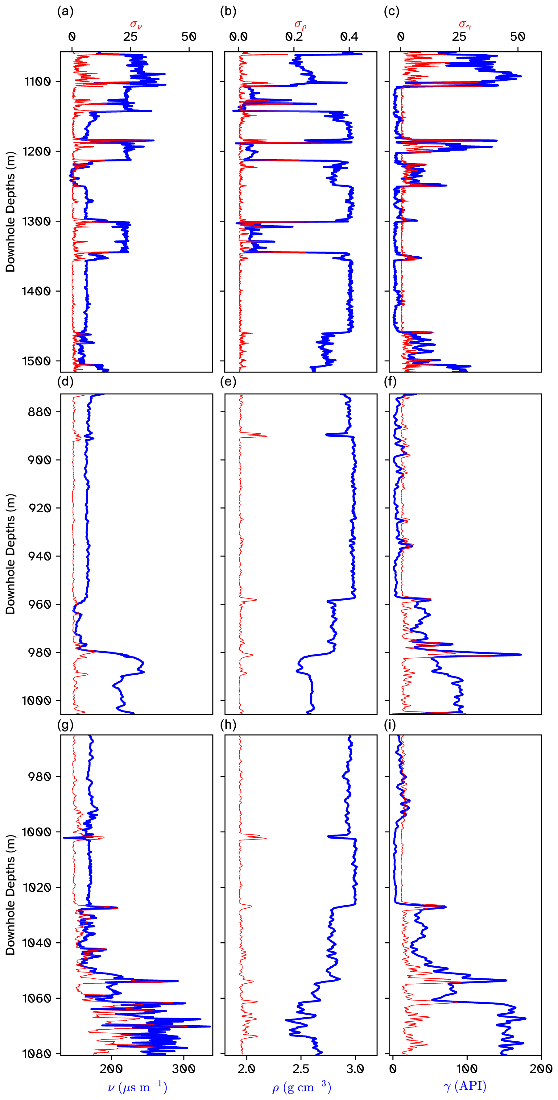
Figure 1 Measured logs for KSL133 (a–c), KSL131 (d–f), and KSL136 (g–i). Panels (a), (d), and (g) show the sonic log; panels (b), (e), and (h) show the gamma–gamma density log; and panels (c), (f), and (i) show the gamma-ray log. Measured values are shown in blue along with the rolling standard deviation for a 1 m window in red.

3.4 Spectral processing

In addition to the standard white-reference normalisation, lens correction and sensor co-registration described by Thiele et al. (2024a), the hyperspectral data were further preprocessed to (1) remove noisy bands, (2) reduce illumination effects that result from the 3D geometry of the scanned drill cores (e.g. shadowing), and (3) enhance mineralogically significant absorption features (Fig. 2).

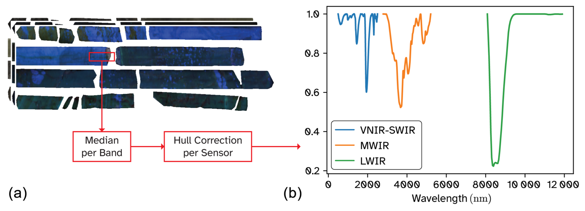
Figure 2 Preprocessing of the hyperspectral data. The images in (a) show an example set of core scans, with the long-wave infrared being shown at the top as a false colour composite. The red rectangle is an example window measuring 100 pixels wide by 50 pixels tall, centred along the core. The spectra within this window are averaged (using a median) and hull-corrected to give the spectrum in (b).

Specifically, the VNIR–SWIR data were subset to the range between 500 and 2500 nm, while the first and last 10 bands of the MWIR and LWIR data were also removed. A hull correction was then applied to the spectra from each sensor separately, using hylite (Thiele et al., 2021), which simultaneously amplifies spectral absorption features and suppresses confounding variability associated with drill core shape and associated inhomogeneous illumination.

3.5 Data balancing

The petrophysical and associated hyperspectral data form distinct clusters, as clearly shown when they are plotted in the petrophysical property space (Fig. 3a). After using the rolling standard deviation to remove high-variance points and associated mixed measurements (Fig. 3b), these clusters are even more distinct. Importantly, the cluster sizes are unbalanced due to different thicknesses of the lithologies in the boreholes, leading to an over-representation of abundant units in the training dataset.

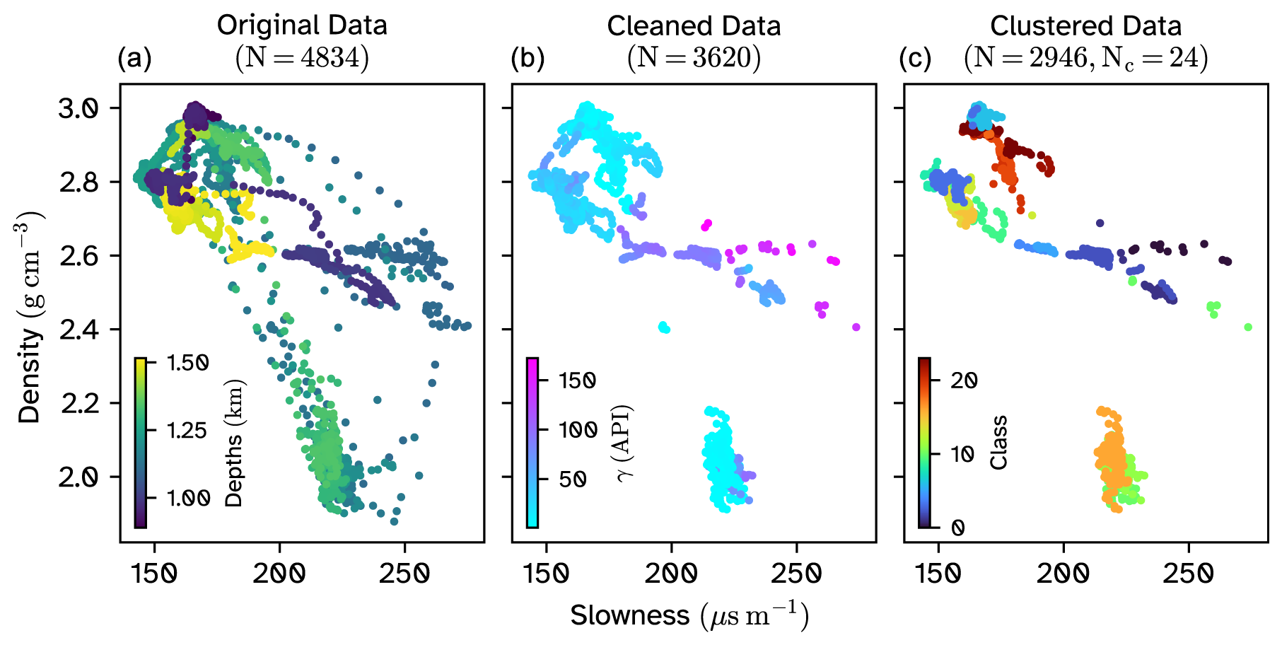
Figure 3 Preprocessing of the training dataset. Slowness–density scatter plots of (a) original dataset, (b) filtered dataset with high-standard-deviation points removed, and (c) the clustered dataset with HDBSCAN class labels. N refers to the number of points in the dataset at the current stage of processing, and N_c refers to the number of clusters defined by the HDBSCAN algorithm (excluding the noisy cluster).

The Hierarchical Density-Based Spatial Clustering of Applications with Noise (HDBSCAN) algorithm was used to identify these clusters and mitigate their translation (as representation bias) into the deep learning models. HDBSCAN is well adapted for its ability to identify clusters of varying densities (McInnes et al., 2017). We used HDBSCAN to automatically identify clusters in a dimensionality-reduced feature space containing the depths of each measurement (to include a spatial component) and the 30 normalised principal components of the median spectra for each data point. This clustering resulted in a total of 24 distinct groups, with one additional noisy cluster excluded from the dataset (Fig. 3c) to leave 2946 remaining spectrum–property pairs. Hyperparameters of HDBSCAN were selected manually and iteratively assessed based on the number and separation between the clusters shown in Fig. 3. We aimed to over-segment the dataset, as the clustering was solely used to help in removing the inherent bias from a larger number of points belonging to one lithology. Any cluster distribution with over-segmented clusters (i.e. the large clusters separated from the rest) would provide similar results during training.

A stratified sampling strategy using the labels from the HDBSCAN clusters was then employed to select well distributed training and validation subsets from drill cores KSL131 and KSL133 (KSL136 was kept separate for independent testing), using a sixfold-stratified train–validation split implemented by the StratifiedShuffleSplit utility in scikit-learn (Pedregosa et al., 2011). This stratification ensures the data diversity is captured in both the train and validation datasets, while a weighted loss function was developed (see Sect. 3.6) to ensure the differing cluster sizes do not bias our model.

3.6 Model architecture and loss function

Our model was developed using PyTorch, an open-source machine learning framework known for its flexibility and strong support for deep learning applications (Paszke et al., 2019). We implemented a multi-headed variant of a 1D convolutional neural network (CNN) architecture (Albawi et al., 2017). The 1D CNN enhances feature extraction by incorporating convolutional layers within a multi-layer perceptron (MLP) framework, using kernels with learnable weights that are convolved with the input data (LeCun et al., 2015).

Each spectral range – VNIR–SWIR, MWIR, and LWIR – was assigned a separate head within the CNN (Fig. 4) to allow for sensor-specific feature extraction. This configuration was chosen to accommodate the different spectral sampling resolutions provided by each sensor and the distinct spectral characteristics associated with each of the respective spectral ranges. By tailoring the kernel sizes to each spectral range, the model was better adapted to identify and capture relevant features across the diverse spectral data. The extracted features were then concatenated and fed through additional fully connected layers before outputting the petrophysical predictions. To ensure balanced contributions from each of the three outputs during loss computation, the slowness, density, and gamma-ray counts were normalised by factors of 10⁻³, 10⁻¹, and 10⁻³ respectively, to ensure that their values fall between 0 and 1.

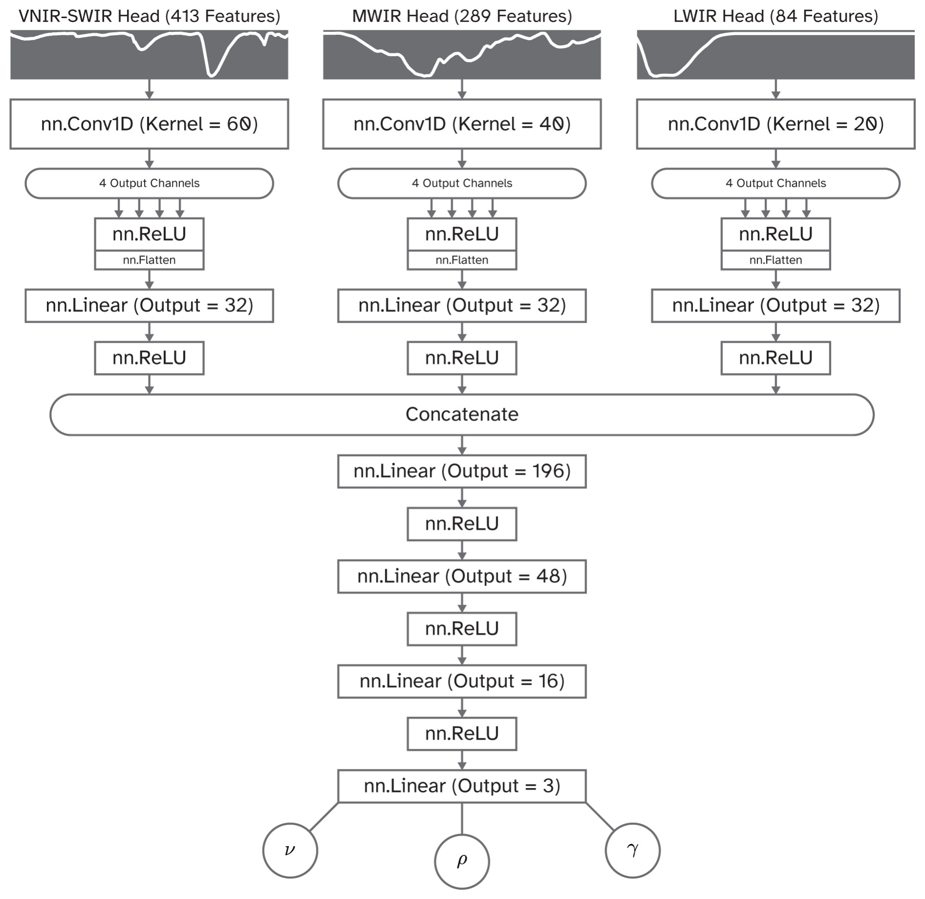
Figure 4 The architecture of the best-performing multi-headed CNN model. Note the difference in convolutional kernel sizes for the different heads. As the number of bands and the shape and size of the absorption features are different across different sensors, the convolutional kernel sizes of 60, 40, and 20 were chosen to better facilitate feature extraction.

A mean squared error (MSE) loss function was used for training, with the following key adjustments. First, to address the imbalance in the number of data points per cluster, we multiplied each output loss by a factor inversely proportional to the number of points in its assigned cluster (see Sect. 3.5). This modification ensured that the model treated each cluster equally, avoiding the disproportionate influence of more populous clusters. Each data point in the kth cluster was associated with a weight w_k given by

$$\begin{array}{}\text{(4)}& {\displaystyle }{\displaystyle }{w}_k={\displaystyle \frac{N_k^{-\mathrm{1}}}{{\sum }_{j=\mathrm{1}}^{N_{\mathrm{c}}}{N}_j^{-\mathrm{1}}}},\end{array}$$

where N_k is the number of points in the kth cluster in the training set, and N_c is the total number of clusters.

Secondly, we introduced a penalty term into the loss function that discouraged negative outputs, as none of the predicted properties can be negative. This ensures that the model predictions stay within valid (positive) bounds by increasing the loss in proportion to the square of the sum of all negative outputs. A penalty term was used instead of, for example, a ReLU activation function to avoid issues with “dying neurons” in the final layer (Lu et al., 2019). The final loss function utilised for training was thus

$$\begin{array}{ll}{\displaystyle }\text{Loss}=\sum _{i=\mathrm{1}}^n& {\displaystyle }[{\displaystyle \frac{\mathrm{1}}{n}}\left(w_i\left(\mathbf{m}\left(x_i\right)-y_i\right)\right)\\ \text{(5)}& {\displaystyle }& {\displaystyle }+\mathit{\lambda }\left(\text{max}\left(-\mathbf{m}\left(x_i\right),\mathrm{0}\right)\right)],\end{array}$$

where m is the model, x_i is the input spectrum, y_i denotes the corresponding petrophysical properties, λ is the penalty factor for negative outputs, n is the batch size, and w_i is the cluster-defined weight (Eq. 4) associated with the ith datum.

The training dataset was shuffled and split into six parts, with the model trained iteratively on each split. Every 100 epochs, a new split was introduced for training and validation, effectively reshuffling the data to help prevent overfitting. Over 600 total epochs, the model iteration with the lowest validation loss was chosen as the best-fitting model. The use of StratifiedShuffleSplit preserved data distribution across splits, reducing overfitting without needing dropout layers or batch normalisation, common in CNNs but sometimes performance-limiting. As mentioned previously, a spatially separated borehole (KSL136) was then used to test the model and evaluate its accuracy after the training phase was completed.

3.7 Shapley analysis

Finally, to help understand the spectral properties that influenced the model predictions, we performed a Shapley value analysis. Shapley values are derived from cooperative game theory and have been widely employed in the machine learning context to quantify each input feature's contribution to model predictions (Lipovetsky and Conklin, 2001). We apply Shapley values using the Python package shap (SHapley Additive exPlanations) (Lundberg and Lee, 2017), specifically leveraging the DeepExplainer utility optimised for deep learning models. This allowed us to efficiently compute feature impacts, enhancing interpretability and transparency in our neural network.

To reduce computational complexity, we subsampled the data before computing Shapley values, selecting 10 random samples from each of the HDBSCAN clusters. This ensures that the samples extracted for Shapley analysis are representative of the entire dataset. We then visualised the results in the form of a raster image to help qualitatively assess the spectral regions used by the model for each of its predictions. Lastly, to better understand the impact of certain bands on the outputs, we computed the mean Shapley values for the top 10 % of each predicted output, to explore which factors resulted in a sample being predicted to be fast (i.e. bottom 10 % of the slowness), be dense, or exhibit high gamma-ray counts.

4 Results

4.1 Model accuracy

The model predictions for the training set showed scores of 0.990, 0.996, and 0.964 for the slowness, density, and gamma-ray values respectively (Fig. 5), suggesting the model explains more than 96 % of the petrophysical variance in the training set. The corresponding root-mean-squared error (RMSE) for these properties was 2.544 µs m⁻¹, 0.023 g cm⁻³, and 4.993 API respectively.

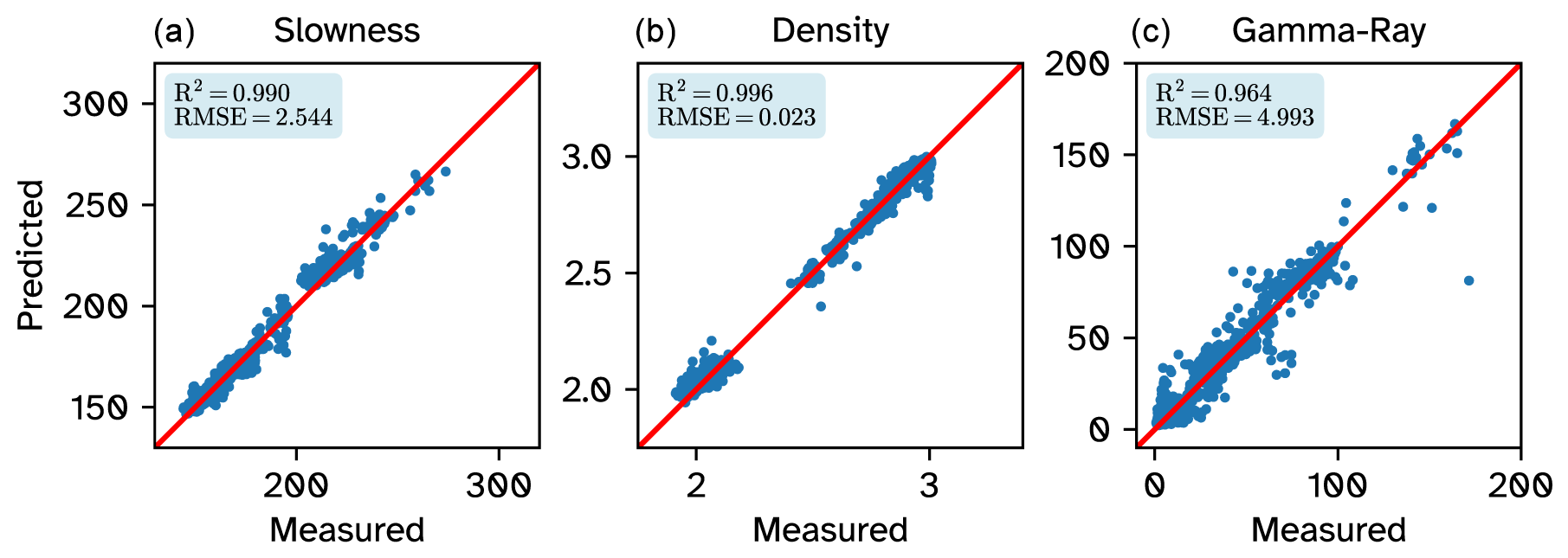
Figure 5 Scatter plots of the measured vs. predicted properties for the training dataset. (a) Slowness (in µs m⁻¹), (b) density (in g cm⁻³), and (c) gamma-ray values (in API).

To better assess the model's accuracy for upscaling applications, we applied it to every 1 mm² pixel in the hyperspectral dataset (including the test drill core), to create a high-resolution (upscaled) map of the petrophysical properties. The results identify fine-scale and cross-core variations that could not be captured by traditional running log measurements (Fig. 6).

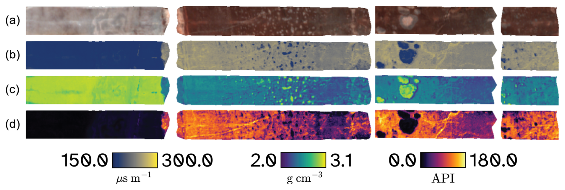
Figure 6 Pixel-scale petrophysical property predictions for an example core scan from the KSL133 borehole. (a) RGB image (derived from the RGB bands of the VNIR sensor), (b) slowness, (c) density, and (d) gamma-ray values.

Our workflow for hyperspectral downsampling (see Sect. 3.3) was then run on these petrophysical property prediction maps to derive an estimate of the petrophysical logging data (noting that the predicted properties slowness, density, and gamma-ray readings are all additive, so they can be arithmetically averaged).

The resulting predicted logging data showed a close match to the measurements (Fig. 7), both for the two training boreholes and for the independent test hole (KSL136). R² scores for this test hole were 0.86 and 0.9 for the density and gamma-ray logs respectively, indicating very reasonable accuracy on unseen data, which even included a basement lithology that was not sampled by the other training drill cores (highlighted by the grey box labelled Tonschiefer i.e. argillaceous basement). The slowness prediction in KSL136 showed a relatively lower R² score of 0.7, with most of the erroneous predictions lying within the unseen lithology. The measured sonic log here shows significant fluctuations, whereas our model prediction remains steady (suggesting the lithology is spectrally quite uniform).

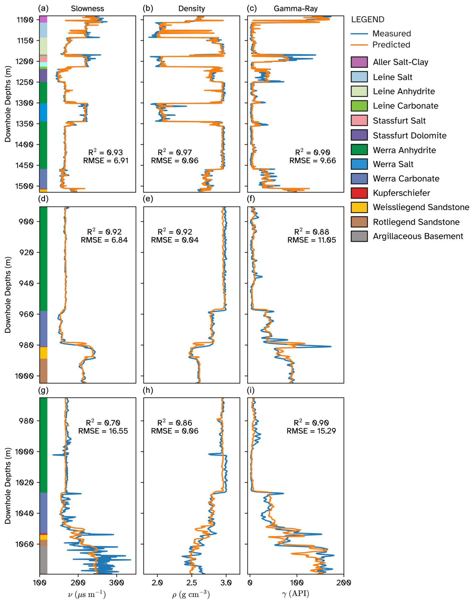
Figure 7 Reconstructed downhole logs for KSL133, KSL131, and KSL136. Panels (a)–(b) show the slowness, density, and gamma-ray values for the KSL133 borehole; (d)–(f) for the KSL131 borehole; and (g–i) for the KSL136 borehole. The coloured rectangles in plots (a), (d), and (g) are the lithologies acquired from the geological logs of the three boreholes.

4.2 Shapley analysis

The calculated Shapley values (Fig. 8) represent the quantitative importance of every input feature in the form of a push away from the mean prediction. Since the theoretical foundation of Shapley analysis looks at every band as a separate feature and not necessarily the overall shape of the absorption feature itself, the overall contribution from a particular spectral range cannot be ascertained from looking at the raw Shapley values. However, a single band in the LWIR, on average, contributes more towards the output than a single band in the VNIR–SWIR–MWIR ranges.

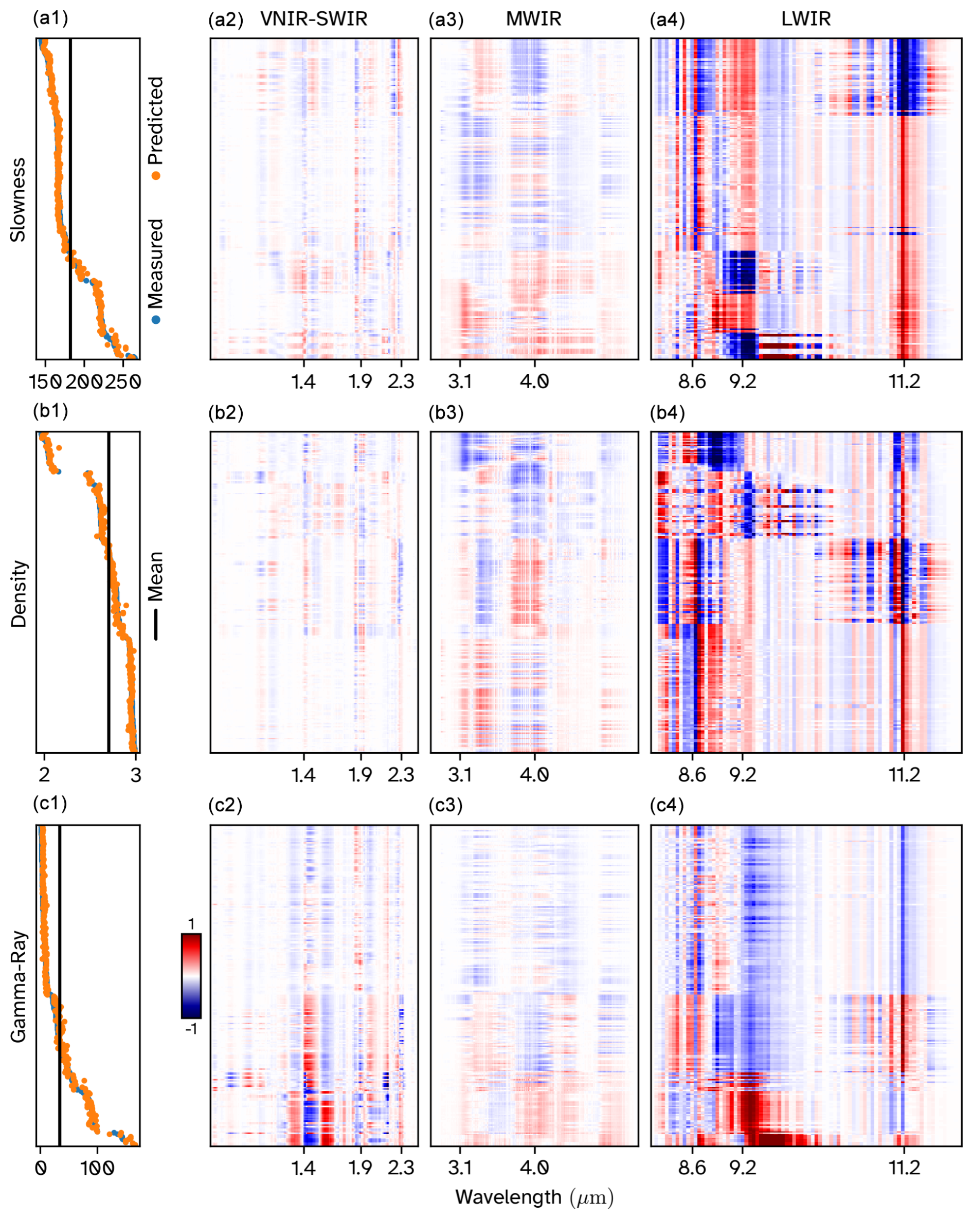
Figure 8 Shapley values for our model. Every row within a sub-figure corresponds to one input spectrum (i.e. a “sample”), and every column corresponds to a particular band within the input spectrum. Panels (a1), (b1), and (c1) show the measured and predicted slowness (in µs m⁻¹), density (in g cm⁻³), and gamma-ray values (in API) respectively (sorted in decreasing order of predicted value). The black vertical line corresponds to the mean predicted output. Panels (a2)–(a4) show the Shapley values for the VNIR–SWIR bands, (b2)–(b4) for the MWIR bands, and (c2)–(c4) for the LWIR bands. Wavelengths at which key absorption features are expected have been annotated along the x axis of these plots.

To look at the total contribution each spectral range makes towards the output, we use the additive nature of Shapley values to create a stack plot (Fig. 9). The plot shows that the contributions from the VNIR–SWIR range are minimal in all predictions. The net contribution from the MWIR bands is the largest, followed by the LWIR bands for slowness predictions, except for the fastest samples, where the LWIR contribution exceeds that of the MWIR bands. For the density predictions, the MWIR dominates the predictions across all the samples, closely followed by LWIR. For the gamma-ray values, the SWIR bands contribute more than in the other two properties, but the LWIR appears to be the dominant steerer of the predicted value.

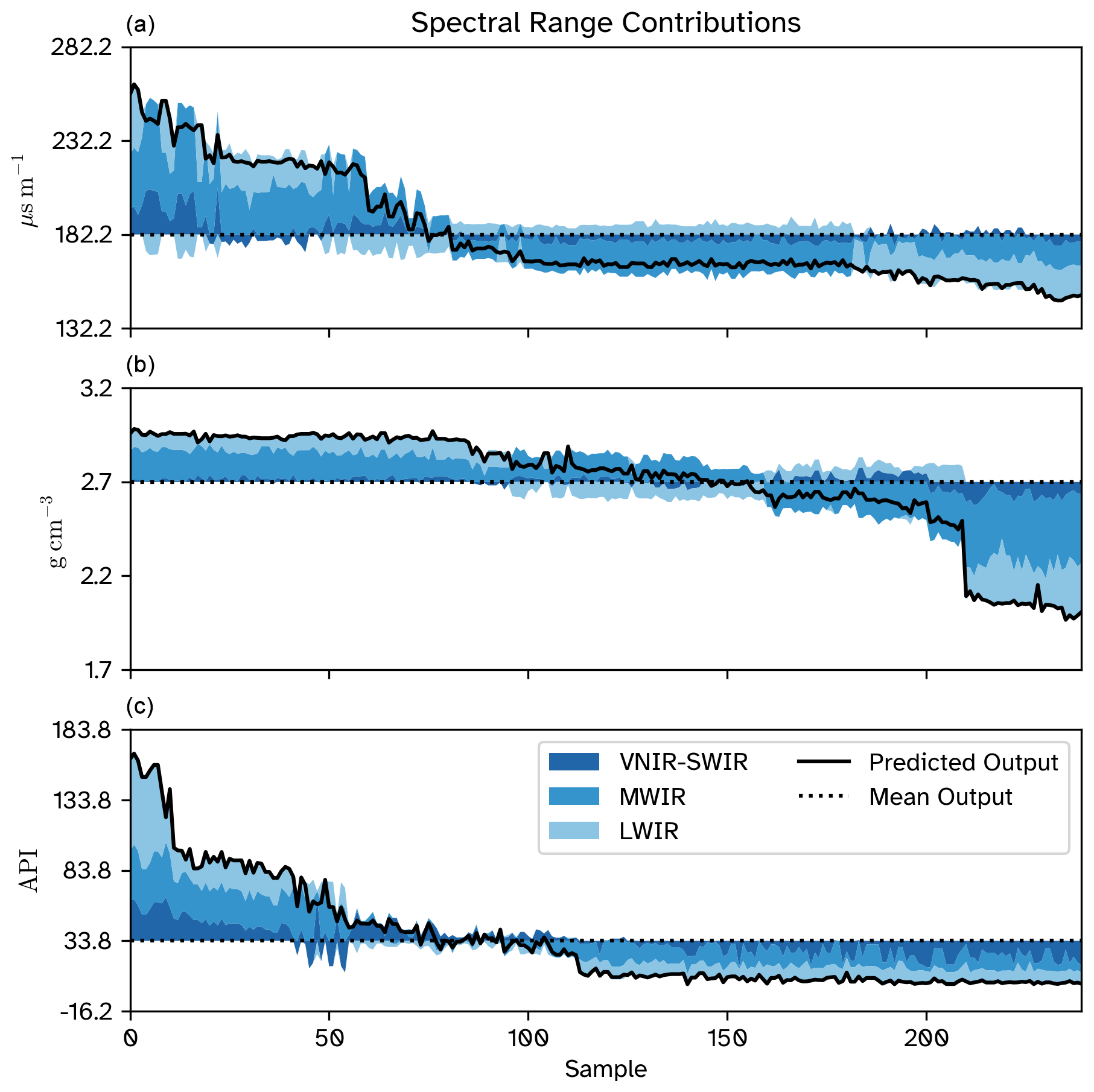
Figure 9 Contribution of each spectral range towards the output. The contribution from each spectral range is calculated by taking the signed sum of all the Shapley values corresponding to the bands in that range for all the input spectra (referred to as “Sample”). The dotted line shows the mean predicted output, and the solid line shows the predicted output value, which is the signed sum of the mean and the individual spectral range contributions.

The median Shapley values of the samples in the bottom 10 % of the slowness predictions (i.e. fastest predicted P wave velocities), the top 10 % of density predictions, and the top 10 % of gamma-ray predictions were calculated as well (Fig. 10). The hull-corrected spectra for these samples (Fig. 11) were then inspected to identify possible spectral features associated with fast, dense, or high gamma-ray predictions. From Fig. 10, it is clear that the model is focusing on known mineral absorption features (and their surrounding bands) in each of the spectral ranges. These include, but are not limited to, the carbonate absorption feature at 11 200 nm, as well as the fundamental overtones of the silicon oxide (νSiO) absorption feature at 8575 and 9200 nm. The 1400 and 1900 nm water and 2200 AlOH SWIR absorption features are also clearly being used, as are the bands around 2300 nm (which are likely influenced by the relatively broad carbonate absorption at 2345 nm).

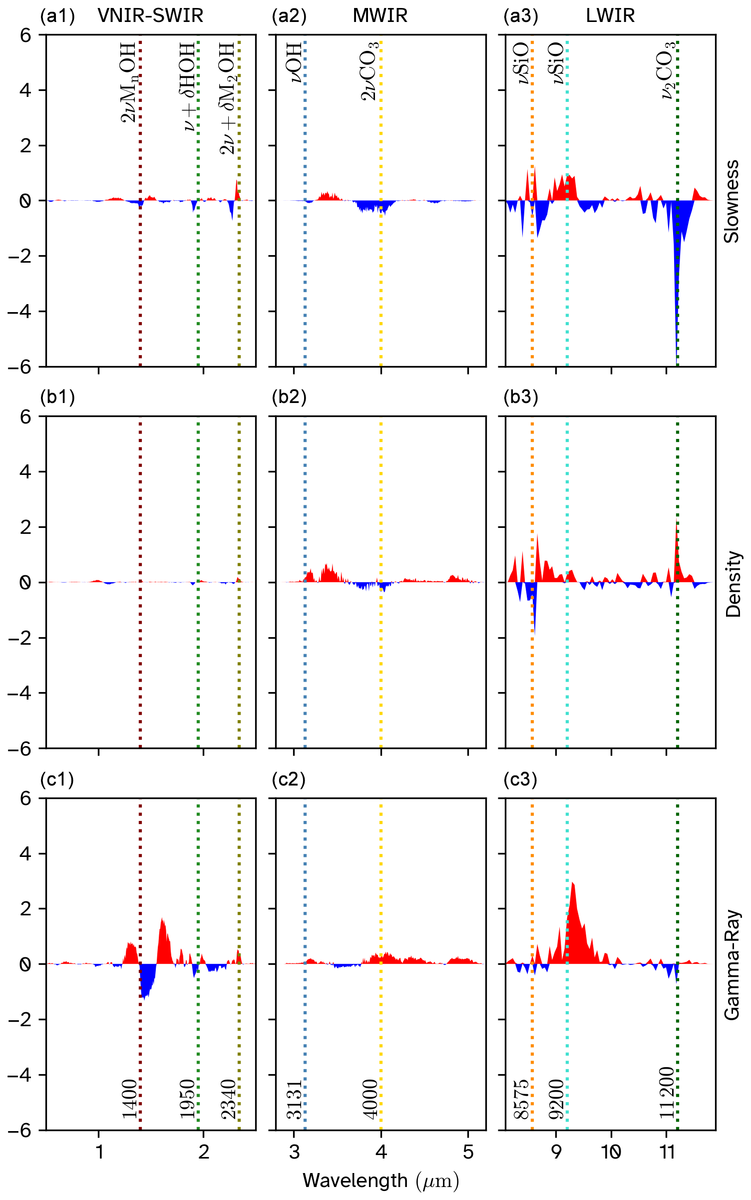
Figure 10 Median of the Shapley values for the selected samples. The columns are split according to the sensors, while the rows are split according to the properties, with (a) showing the median Shapley value for slowness, (b) for the density, and (c) for the gamma-ray values. The red regions correspond to the bands that push the output above the mean, whereas the blue regions correspond to the bands that push the output below the mean. The dotted vertical lines mark the key absorption features of interest within an IR spectrum (Laukamp et al., 2021), with the annotations specifying the wavelength (in nm) and the corresponding molecular vibrational features.

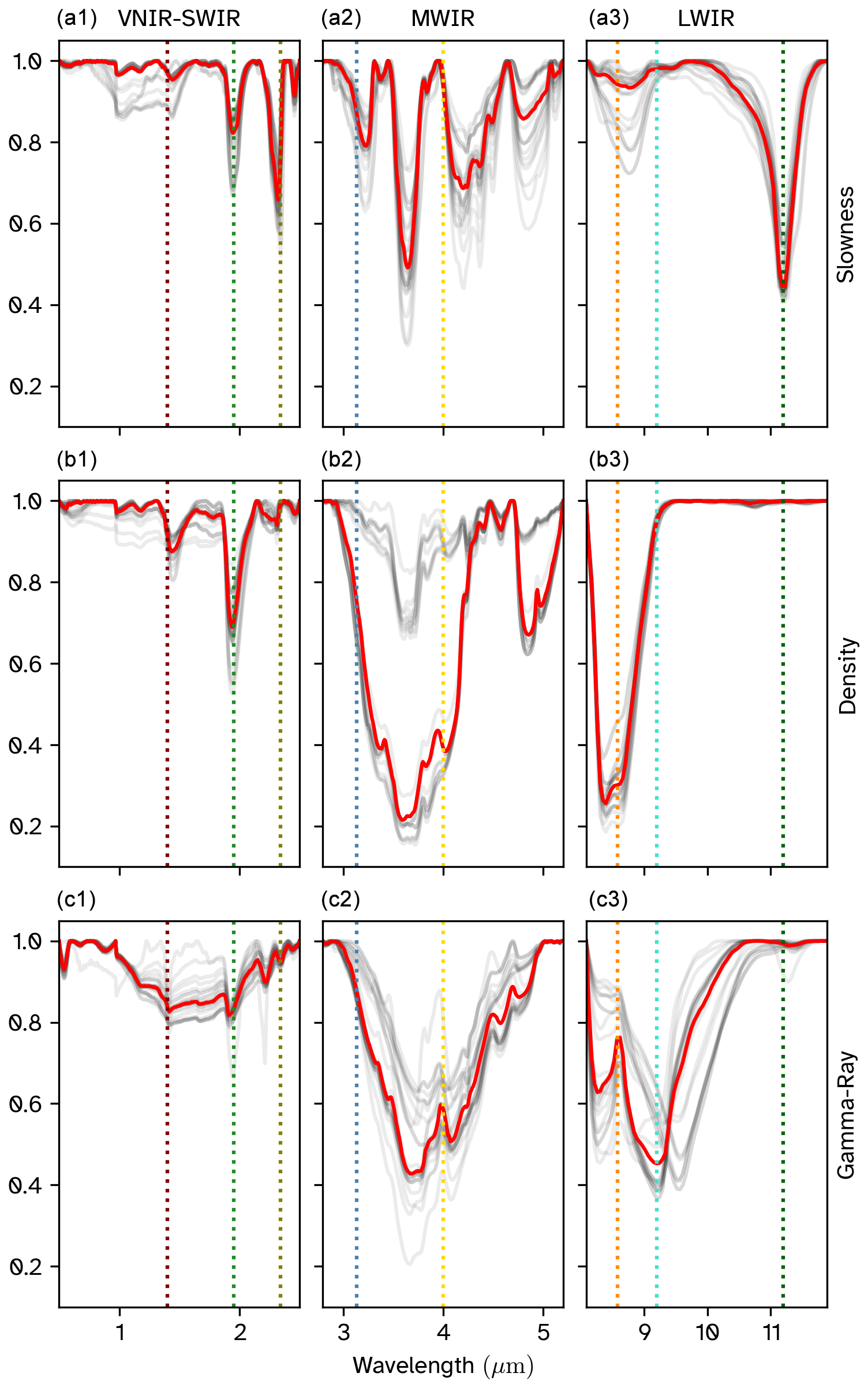
Figure 11 Reflectance spectra of selected samples. The columns are split according to the sensors, while the rows are split according to the properties, with (a) showing the spectra of the samples in the bottom 10 % of slowness predictions, (b) showing the spectra of the samples in the top 10 % of density predictions, and (c) showing the spectra for the samples in the top 10 % of gamma-ray reading predictions. The low-opacity grey lines plot the individual spectra, whereas the red line corresponds to the median spectrum.

The results highlight some spectral variability within these top 10 % groups, as would be expected, but also some commonalities. For instance, in the slowness plots (Fig. 10a), the samples show a significant push below the mean due to the bands around 11 200 and 4000 nm, corresponding to primary and secondary overtones of carbonate absorption features. This observation aligns with our geological understanding, as the fastest samples are from the Stassfurt dolomite formation (see legend, Fig. 7). The spectra in Fig. 11a further support this inference, as they exhibit a clear carbonate absorption feature.

Conversely, the densest samples in the region are associated with the Werra Anhydrite formation (see legend, Fig. 7). They do not exhibit the carbonate absorption feature as seen in the spectra (Fig. 11b), and the low Shapley values for those bands (Fig. 10b) confirm that the model is no longer looking at any of the carbonate absorption features.

The samples with the top 10 % of gamma-ray readings come from the Aller salt clay formation, the Stassfurt salt formation, and the Rotliegend sandstone formation. The model considers the bands corresponding to the water absorption feature, as well as the clay feature in the SWIR favourably (Fig. 10c). Furthermore, there is a considerable peak in the 9200–9600 nm range in the LWIR, which might correspond to the tecto- and sheet-silicate absorption features (Laukamp et al., 2021) containing potassium salts from the Aller salt clay and Stassfurt salt formations, or the K-feldspar absorption feature from the Rotliegend sandstones, both of which would give rise to high gamma-ray values.

5 Discussion

Our deep learning approach has managed to accurately predict the variability in petrophysical properties from hyperspectral data. This prompts several important questions: what is the model using to make these predictions? Are the results potentially generalisable or likely only valid for cores from the Spremberg area? And how could this novel approach help improve our understanding of, and ability to predict, subsurface behaviour?

The Shapley values (Figs. 8–10) clearly indicate that the model is extracting features associated with the depth and shape of known mineral absorption features, especially those relating to quartz, feldspars, and carbonates in the LWIR range. This suggests a primary sensitivity to mineralogy, which we suggest is reasonable given the mineralogical control on all the predicted petrophysical properties. The model also clearly places a strong emphasis on the MWIR and the LWIR bands, even though much of the mineralogical variation could also be identified using these other spectral ranges. Based on this, we speculate that the model could be learning to identify relatively subtle changes in LWIR absorption feature shape that are known (Zaini et al., 2012; Rost et al., 2018; Salisbury et al., 1987) to vary with grain size and surface roughness (which we suggest is likely correlated to porosity).

Importantly, the Shapley values for predicted gamma emission differ substantially, presumably as gamma emission is primarily controlled by mineralogy. Gamma-ray emissions are triggered by natural radioactive decay of elements like potassium, thorium, and uranium (Asquith et al., 2004). These are typically hosted in clay (and feldspar) minerals so the SWIR bands, especially those around 1400 nm (associated with hydrated minerals) and 2340 nm (related to clay minerals), are expected to play a more prominent role for gamma prediction. The increased Shapley values in these regions indicate that the model is correctly associating higher absorption at these wavelengths with elevated gamma-ray values, as expected in shaly rocks or clays. Similarly, the predicted gamma emissions do not appear sensitive to many of the spectral regions used to predict density and slowness, such as the carbonate feature at 11 200 nm.

A common challenge for deep learning models based on CNNs is whether or not they can be generalised. In this study, training and applying the model to three drill cores from the same geological sequence does not mean that similar results could be attained in different geological sequences. However, given the results from our Shapley value analysis, we suggest that it is unlikely that the model is “just” learning to distinguish different lithologies and returning appropriate (average) predictions. Instead, it appears to generate predictions based on the mineralogical and textural information captured by the spectra. This is key to its demonstrated ability to identify intra-lithology variations in each of the petrophysical properties (Fig. 7) and possibly explains why it produced broadly reasonable predictions for the unseen basement lithology. The model appears to be sensitive to the fundamental mechanical and petrophysical properties of the rock, which suggests that it could be generalised on more diverse data. Hence, while we would not apply our model outside of the Spremberg region (given its very limited training), it appears that our approach could be applied, given appropriate training information, to derive more widely applicable predictions.

While a generalised model would require significantly more training data (and rigorous evaluation), we suggest that locally trained models such as the one presented here can be very useful. The translation of ≈ metre-scale petrophysical logger measurements to millimetre-resolution maps provides significantly more detail on the physical and mechanical structure of the sampled rock mass. This combination of large extent and high spatial resolution helps to address the scaling challenges commonly encountered when extrapolating properties measured at a small scale (using ≈1–10 cm sized laboratory tests) to larger, reservoir-scale models (Christie, 1996).

We suggest that the information on mesoscale heterogeneity captured by these hyperspectral predictions could be used to bridge the scale gap between laboratory and reservoir properties. Further tests in different settings are required to confirm this assumption. The extensive literature describes various solutions to this scaling problem. Traditional approaches, including statistical averaging, renormalisation techniques, and geostatistical methods, have been employed to derive effective medium parameters suitable for reservoir simulations (Renard and de Marsily, 1997; King, 1989). Our work introduces a novel approach that leverages hyperspectral data as an intermediary between different measurement resolutions. By integrating hyperspectral data with traditional petrophysical data, we can capture fine-scale heterogeneity (at ≈1 mm² resolution; Fig. 6) while retaining coverage applicable at the reservoir scale (extent of several hundred metres). A similar approach might also be possible using outcrop hyperspectral data, if data quality issues associated with hyperspectral outcrop imaging can be resolved, further improving our ability to quantify mesoscale mechanical and petrophysical variability and so linking laboratory- and reservoir-scale properties.

6 Conclusions

To conclude, our results demonstrate the link between hyperspectral and petrophysical properties. We have developed a preprocessing workflow that overcomes challenges associated with differing data resolutions and successfully trained a deep learning model to predict slowness, density, and gamma-ray count from VNIR, SWIR, MWIR, and LWIR hyperspectral data. We effectively super-resolve the borehole petrophysics data (i.e. from ≈0.1 m resolution of the logger to 0.001 m resolution of the hyperspectral cameras), which helps us explore the intricacies and variations of these properties that cannot be captured by running log measurements. Additionally, our workflow mitigates the co-registration uncertainties that prevent machine learning workflows from being carried out over drill core data. The model was tested on an independent drill core, which included an unseen lithology, and gave accurate predictions (test R² score >0.7). A Shapley analysis suggests the model is leveraging the sensitivity of the MWIR–LWIR range to mineralogy, grain size, and surface roughness to inform predictions of slowness and density, indicating that some degree of generalisation might be possible. The gamma predictions are much more closely linked to mineralogy, so they could be quite broadly applicable.

We suggest that this novel approach enables the quantification of petrophysical properties at high spatial resolution over large areas, providing the information on mesoscale heterogeneity needed to help bridge laboratory- and reservoir-scale mechanical and physical behaviour. Our work also serves as a stepping stone toward predicting secondary properties such as porosity and permeability, helping build a link between hyperspectral data and widely used physical rock property measurements.