About the trustworthiness of physics-based machine learning – considerations for geomechanical applications

Model predictions are important to assess the subsurface state distributions (such as the stress), which are essential for, for instance, determining the location of potential nuclear waste disposal sites. Providing these predictions with quantified uncertainties often requires a large number of simulations, which is difficult due to the high CPU time needed. One possibility for addressing the computational burden is to use surrogate models. Purely data-driven approaches face challenges when operating in data-sparse application fields such as geomechanical modeling or producing interpretable models. The latter aspect is critical for applications such as nuclear waste disposal, where it is essential to provide trustworthy predictions. To overcome the challenge of trustworthiness, we propose the usage of a novel hybrid machine learning method, namely the non-intrusive reduced-basis method, as a surrogate model. This method resolves both of the above challenges while being orders of magnitude faster than classical finite element simulations. In the paper, we demonstrate the usage of the non-intrusive reduced-basis method for 3-D geomechanical–numerical modeling with a comprehensive sensitivity assessment. The usage of these surrogate geomechanical models yields a speed-up of 6 orders of magnitude while maintaining global errors in the range of less than 0.01 %. Because of this enormous reduction in computation time, computationally demanding methods such as global sensitivity analyses, which provide valuable information about the contribution of the various model parameters to stress variability, become feasible. The opportunities of these added benefits are demonstrated with a benchmark example and a simplified study for a siting region for a potential nuclear waste repository in Nördlich Lägern (Switzerland).

1 Introduction

Knowledge of the crustal stress field is of key importance for the safe usage of the subsurface, for example, for geothermal exploitation or storage of energy, CO₂, and nuclear waste (Blöcher et al., 2018; Henk, 2008; Hergert et al., 2015; Smart et al., 2014). The importance is expressed in the unwanted release of stored elastic energy during anthropogenic utilization by means of failure of boreholes (Schmitt et al., 2012; Tingay et al., 2008), caverns, and tunnels (Brady and Brown, 2006); subsidence; or induced seismic events (Ellsworth, 2013; Segall and Fitzgerald, 1998; Ziegler et al., 2015). Thus, to develop strategies that reduce the risks of induced hazards and prevent failure due to human-made interventions in the subsurface, it is important to understand the undisturbed 3-D in situ stress state (Gaucher et al., 2015). However, the in situ stress state is challenging to quantify. Stress data are rare; often subject to large uncertainties; and describe, in most cases, only a subset of the six independent components of the symmetric second-rank tensor that formally describes the stress state at an arbitrary point in the subsurface (Amadei and Stephansson, 1997; Desroches et al., 2021; Heidbach et al., 2018; Morawietz et al., 2020).

To obtain a continuous description of the 3-D stress tensor in a given rock volume, geomechanical–numerical models are employed. These models usually use the finite element method to solve the partial differential equation that describes the equilibrium of forces (e.g., Ahlers et al., 2021; Fischer and Henk, 2013; Lecampion and Lei, 2010; Reiter and Heidbach, 2014; Singha and Chatterjee, 2015; van Wees et al., 2018). For the model input, we have to describe the rock properties, the boundary conditions, and the subsurface geological structures. However, knowledge about these parameters is usually incomplete and consequently associated with uncertainties (e.g., Hergert et al., 2015; Ziegler and Heidbach, 2020). This means that for providing reliable model predictions the information regarding these parameter variabilities needs to be included and assessed.

Such tasks are commonly achieved through global sensitivity analyses (SAs; Degen et al., 2021a, b; Saltelli et al., 2019) and uncertainty quantification methods (Degen et al., 2022a, c; Saltelli et al., 2019). Both methods have the requirement of numerous model evaluations in common, which poses major challenges when each model evaluation is computationally costly. One way to circumvent the issue is the use of surrogate models (also referred to as meta or reduced models), i.e., low-order representations of the original model that are significantly faster to compute. Many surrogate model construction techniques exist, ranging from physics-based to data-driven approaches (e.g., Benner et al., 2015; Degen et al., 2023; Hesthaven et al., 2016; Jordan and Mitchell, 2015; Kotsiantis et al., 2007; Mahesh, 2020). Nonetheless, every surrogate model needs to be evaluated concerning its trustworthiness and explainability. This is important for several reasons: (i) if we use the surrogate in subsequent analyses such as global sensitivity analyses, we need to ensure that the surrogate represents the original model, otherwise the obtained sensitivities are not representative; (ii) if the model results are used for decision-making processes, they need to be reliable and robust.

Different techniques exist for the construction of surrogate models, generally subdivided into three categories. In the following we briefly present the various techniques, explaining their key advantages and disadvantages:

1. One class of techniques is the data-driven machine learning approach, which recently gained attention in the construction of surrogate models (e.g., Bergen et al., 2019; Degen et al., 2023; Li et al., 2023; Swischuk et al., 2019; Willcox et al., 2021). This is thanks to their capabilities of approximating well nonlinear applications, their straightforward usage because of their black box and non-intrusive nature (meaning that they do not need direct access to the numerical solver), and their availability in software frameworks such as PyTorch (Paszke et al., 2019) and TensorFlow (Abadi et al., 2015). Nonetheless, the black box nature also has the disadvantage of yielding non-explainable models that do not preserve the governing physical equations, making their utilization challenging in terms of reliability.

2. Physics-based methods such as the reduced-basis method or the proper orthogonal decomposition have the advantage of preserving the physics (Benner et al., 2015; Degen et al., 2020a; Hesthaven et al., 2016; Quarteroni et al., 2015; Rozza et al., 2008). The reduced-basis method has been developed in the field of applied mathematics and has been used for various applications, such as transport and continuum mechanics (e.g., Benner et al., 2015; Hesthaven et al., 2016; Quarteroni et al., 2015; Rozza et al., 2008) and also for large-scale geothermal applications (Degen et al., 2021b, 2022c). However, they reach their limits in efficiently approximating highly nonlinear problems (Degen et al., 2023; Hesthaven and Ubbiali, 2018; Wang et al., 2019, see also Sect. 2).

3. To overcome the limitations of both individual approaches, physics-based machine learning methods are introduced, which combine data-driven and physics-based techniques. Several physics-based machine learning methods are available, and they have different implications concerning the question of explainable surrogate models (e.g., Degen et al., 2023; Faroughi et al., 2022; Willard et al., 2022). In this study, we use the non-intrusive reduced-basis (NI-RB) method (Hesthaven and Ubbiali, 2018; Swischuk et al., 2019) for the construction of the surrogate models for geomechanical applications and demonstrate how it fulfills the criteria of explainable and reliable surrogate models in contrast to other physics-based machine learning techniques.

This paper focuses on two main aspects: (i) the combined consideration of different sources of uncertainty, such as stress magnitude data records used for calibration, material properties, and subsurface geometry, and (ii) the consideration of rapid changes in the state distribution. Especially the later part distinguishes the work significantly from previous studies in geothermal applications (e.g., Degen et al., 2022a), where only smooth-state variable distributions of the pore pressure and/or temperature have been considered so far. Depending on the permeability contrast, the pore pressure exhibits rapid changes as well. However, these scenarios have not yet been investigated with respect to the non-intrusive reduced-basis method. Following a benchmark example the workflow is applied to a data set from northern Switzerland, where an underground repository for nuclear waste is planned.

2 Background and methods

In the following, we present the governing equations for geomechanical–numerical modeling presented in this paper. Afterwards, we introduce the non-intrusive reduced-basis method, which is responsible for constructing the surrogate models. Additionally, we explain the concept of global sensitivity analyses, which are used to investigate the influence of the model parameters.

2.1 Subsurface stress state

The stress state in the subsurface is usually described by the symmetric second-rank stress tensor σ_ij:

$$\begin{array}{}\text{(1)}& {\displaystyle }{\displaystyle }{\mathit{\sigma }}_{ij}=\left(\begin{array}{ccc}{\mathit{\sigma }}_{xx}& {\mathit{\sigma }}_{xy}& {\mathit{\sigma }}_{xz}\\ {\mathit{\sigma }}_{yx}& {\mathit{\sigma }}_{yy}& {\mathit{\sigma }}_{yz}\\ {\mathit{\sigma }}_{zx}& {\mathit{\sigma }}_{zy}& {\mathit{\sigma }}_{zz}\end{array}\right),\end{array}$$

with six independent components – the three normal stresses σ_xx, σ_yy, and σ_zz as well as three shear stresses σ_xy=σ_yx, σ_yz=σ_zy, and σ_zx=σ_xz. Commonly, instead of the full stress tensor, the stress state, in its main axis system which is a rotation of the stress tensor, is referred to in a way that all shear stresses dissipate and only normal stresses remain so that

$$\begin{array}{}\text{(2)}& {\displaystyle }{\displaystyle }\mathbf{S}=\left(\begin{array}{ccc}{S}_{\mathrm{1}}& \mathrm{0}& \mathrm{0}\\ \mathrm{0}& S_{\mathrm{2}}& \mathrm{0}\\ \mathrm{0}& \mathrm{0}& S_{\mathrm{3}}\end{array}\right),\end{array}$$

with the principal stress components S₁, S₂, and S₃ that are perpendicular to each other but arbitrarily oriented in space. A common assumption in upper-crustal geomechanics is that one of the principal stress axes is vertical as a result of the overburden which can then be referred to as S_v (Zoback, 2007). The other two principal stress axes are then by definition horizontal and called the maximum and minimum horizontal stress S_Hmax and S_hmin, respectively. Then the stress state can be fully described by four variables only: the magnitudes of S_v, S_Hmax, and S_hmin as well as the orientation of one of the two horizontal stress components. This is then called the reduced stress tensor (Zoback, 2007).

Information on the orientation of S_Hmax is available from a variety of stress indicators that are, e.g., compiled in the World Stress Map (Heidbach et al., 2018). Stress magnitude data are less frequently available, sparse, and often of little quality (Morawietz et al., 2020). However, in particular, the stress magnitudes are important for many subsurface applications. If detailed information on the in situ stress state is required, 3-D geomechanical–numerical modeling is applied in order to estimate the stress state in a volume of interest based on few data records (e.g., Fischer and Henk, 2013; Lecampion and Lei, 2010; Singha and Chatterjee, 2015; van Wees et al., 2018; Ziegler et al., 2016).

2.2 Governing equations

The modeling of the in situ stress state is conducted under the assumption of a linear elastic upper crust as the governing constitutive equation (Reiter and Heidbach, 2014; Hergert et al., 2015; Singha and Chatterjee, 2015) and no acceleration except for gravity. The required material properties are thus the Young modulus (E), the Poisson ratio (ν), and the density (ρ). We derive the total stress σ from the momentum balance (Cacace and Jacquey, 2017):

$$\begin{array}{}\text{(3)}& {\displaystyle }{\displaystyle }\mathrm{\nabla }\cdot \mathit{\sigma }+\mathit{\rho }g=\mathrm{0},\end{array}$$

where ρ is the density and g the gravity acceleration. The numerical forward simulations are performed in GOLEM (Cacace and Jacquey, 2017), which is an open-source high-performance finite element software based on the MOOSE framework (Lindsay et al., 2022). The result is the full stress tensor σ_ij at discrete locations throughout the model volume. This information is used to derive scalar values such as individual components from the reduced stress tensor or the slip tendency of faults (Röckel et al., 2022). Furthermore, we consider the following constitutive linear elastic relationships:

$$\begin{array}{}\text{(4)}& {\displaystyle }{\displaystyle }E={\displaystyle \frac{\mathit{\sigma }}{{\mathit{\epsilon }}_{\text{axial}}}}\text{and }\mathit{\nu }=-{\displaystyle \frac{{\mathit{\epsilon }}_{\text{trans}}}{{\mathit{\epsilon }}_{\text{axial}}}}.\end{array}$$

Here, ε_axial and ε_trans are the axial and transverses strains, respectively.

The model geometry is usually oriented in a way that the boundaries are parallel and perpendicular to the orientation of S_Hmax and S_hmin (Fig. 1). The stress state is introduced to the model using displacement boundary conditions (Dirichlet-type) on the lateral boundaries of the model. The magnitude of displacements is adapted in a way that the resulting stress magnitudes (S_Hmax and S_hmin) match observed data records (Reiter and Heidbach, 2014; Ziegler and Heidbach, 2020). This process is referred to as the calibration of the model. It is of an iterative nature or aided by the software tool FAST Calibration (Ziegler et al., 2023).

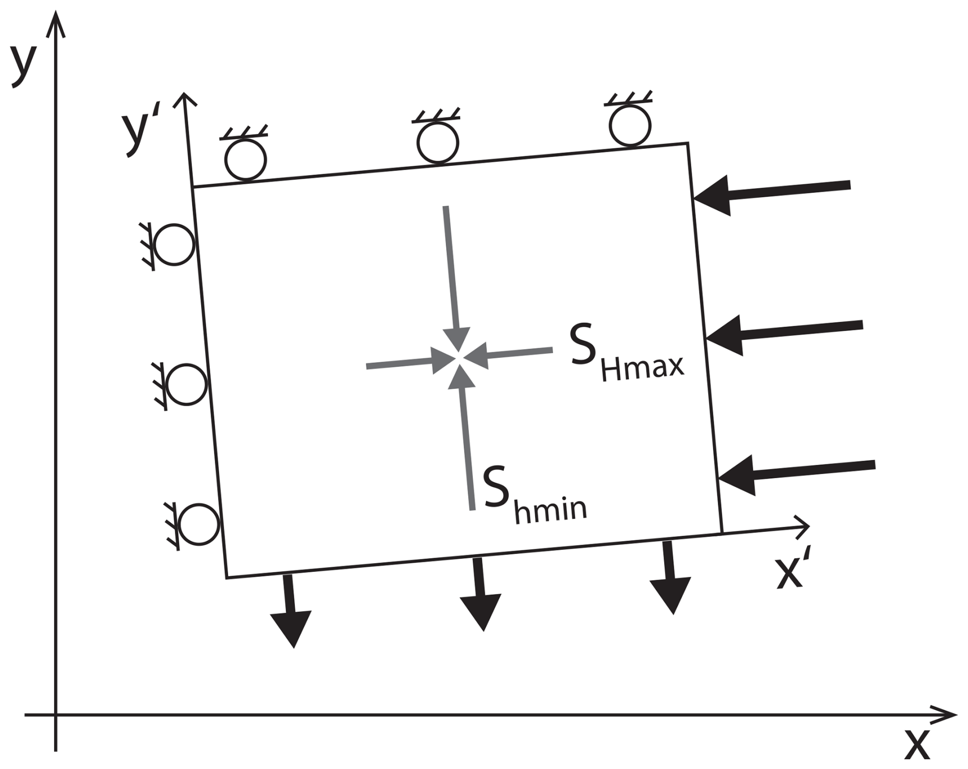
Figure 1 The model setup with the Cartesian model coordinate system (x and y axes) and the coordinate system used for application of boundary conditions (x^′ and y^′ axes) perpendicular to the model boundaries and the orientations of S_Hmax and S_hmin, respectively. The boundary conditions (Dirichlet-type) are indicated by the bold arrows (prescribed displacements) and rollers that indicate a zero displacement perpendicular to the model boundary.

2.3 Non-intrusive reduced-basis method

In this work, we evaluate the trustworthiness of geomechanical surrogate models for use in applications such as nuclear waste disposal. Note that we focus on the construction of surrogate models for the S_hmin, S_Hmax, and S_v components. For better illustration of the general concepts, we assume that the material properties are homogeneous and isotropic within each layer. However, the presented concepts are not restricted to these assumptions. Further details regarding the model setup are listed in Sect. 3. For the purpose of the surrogate model construction, we use the non-intrusive reduced-basis (NI-RB) method to construct the surrogate models (Hesthaven and Ubbiali, 2018; Swischuk et al., 2019; Wang et al., 2019). The NI-RB method combines physics-based and data-driven approaches to provide reliable predictions even for complex nonlinear and hyperbolic partial differential equations (PDEs).

The NI-RB method is most advantageous in the many-query or real-time context, so if either many and/or fast model evaluations are required (Benner et al., 2015; Hesthaven and Ubbiali, 2018; Hesthaven et al., 2016). To ensure this, the method is divided into two stages: the offline and online stages, as illustrated in Fig. 2. During the offline stage, the training data are generated and the surrogate model is constructed. This stage is computationally expensive since it requires several full-order solutions of the model, as we explain in the next paragraph. However, it needs to be performed only once. On the other hand, during the following online stage, the surrogate model is evaluated. This is a computationally fast procedure allowing numerous evaluations of the surrogate model in a short amount of time (Benner et al., 2015; Hesthaven and Ubbiali, 2018).

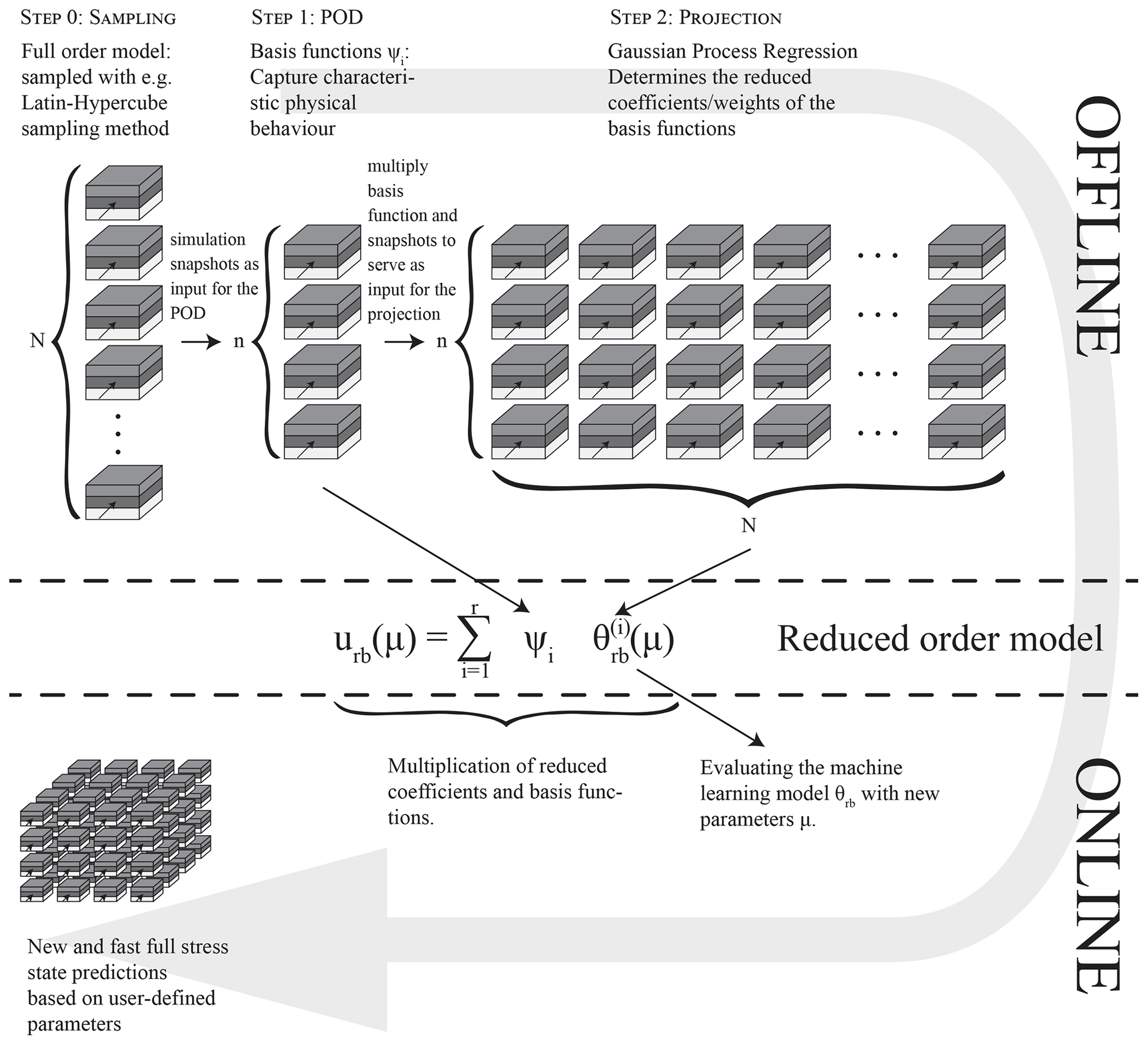
Figure 2 Schematic representation of the offline and online procedure for the NI-RB method, including the different steps required for the model construction in the offline phase. Note that u_rb denotes the reduced solution, μ the model parameters, r the reduced dimension, ψ the basis functions, θ_rb the reduced coefficients, N the total number of samples, and n the number of basis functions.

2.3.1 Offline stage

The construction of the surrogate model in the offline stage is also a two-step procedure, which is preceded by step zero where the model parameters for the full-order solutions are determined (step 0 in Fig. 2). In our case, we use a quasi-random Latin hypercube sampling strategy (Loh, 1996) for the generation of the 100–200 training snapshots with the parameter ranges provided in Table 1. These snapshots are combinations of different geometries, rock properties, and boundary conditions, as shown in Fig. 2.

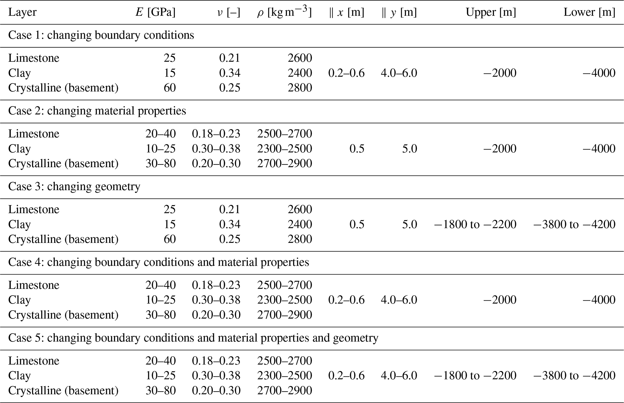
Table 1 Variation ranges of the input parameters for all five cases. Note that ∥x and ∥y denote the displacement for the boundary condition on the x and y axes, respectively. Furthermore, “upper” denotes the interface between the limestone and clay layer and “lower” the interface between the clay and crystalline layer. The parameter ranges have been chosen to be representative of nuclear waste disposal applications (Crisci et al., 2022a, b; Gonus et al., 2022a, b, 2023; Spillmann et al., 2022), and the thickness data are from Crisci et al. (2022a). The Young modulus of the crystalline layers was extended beyond that range to account also for other subsurface engineering applications.

In the first step (Fig. 2) of the offline stage, the basis functions of the surrogate model are calculated by performing a proper orthogonal decomposition (POD). They capture the characteristic physical behavior of the model by regarding the models response to different properties provided by the snapshots. In order to ensure an efficient execution of both the POD and machine learning stage, we scale the input parameters as well as the data sets. The input parameters are transformed using z score normalization, resulting in a mean of 0 and a standard deviation of 1. The training data are scaled with a min–max scaling, taking the maximum and minimum values, which yields a data set distributed between 0 and 1. The basis functions correspond to the most influential singular vectors (Hesthaven and Ubbiali, 2018). For defining this, the energy criterion is used (Guo and Hesthaven, 2019; Swischuk et al., 2019):

$$\begin{array}{}\text{(5)}& {\displaystyle }{\displaystyle \frac{{\sum }_{i=\mathrm{1}}^r{\mathit{\lambda }}_i^{\mathrm{2}}}{{\sum }_{i=\mathrm{1}}^N{\mathit{\lambda }}_i^{\mathrm{2}}}}\le \mathit{ϵ},\end{array}$$

where r corresponds to the dimension of the reduced model, λ to the singular value, N to the total number of samples, and ϵ to the desired accuracy of the surrogate. Since ϵ is a user-defined value, the quality of the surrogate is adjustable to the application. In our case studies, we set the tolerance ϵ to maintain 10⁻⁴ % of the information content to ensure surrogate models that represent the full-order solutions well. This tolerance is application-specific and based on the experience of previous studies (Degen et al., 2023, 2022a, 2020a).

The resulting surrogate model u_rb is a linear combination of basis function ψ determined in step 1 and reduced coefficients θ_rb.

$$\begin{array}{}\text{(6)}& {\displaystyle }{\displaystyle }{u}_{\text{rb}}\left(\mathit{\mu }\right)=\sum _{i=\mathrm{1}}^r{\mathit{\psi }}_i{\mathit{\theta }}_{\text{rb}}^{\left(i\right)}\left(\mathit{\mu }\right)\in V_{\text{rb}}\end{array}$$

Here, μ refers to the model parameters and V_rb to the reduced space. The determination of these coefficients is the second step of the offline phase, which is classically performed by a Galerkin projection (Benner et al., 2015; Hesthaven et al., 2016; Quarteroni et al., 2015). However, to allow also for a later extension to nonlinear applications, we use in this study machine learning methods to determine the coefficients instead (step 2 in Fig. 2). This possible extension to the nonlinear setting is shown in several studies (Degen et al., 2022a; Hesthaven and Ubbiali, 2018; Swischuk et al., 2019). In the present study, we use Gaussian process regression (GPR; Schulz et al., 2018) as the machine learning method, which works better than neural networks in a linear setting since fewer hyperparameters need to be determined. We use anisotropic radial basis function kernels with an initial length scale of 1, which is optimized for each normalized model parameter μ within the ranges of 10⁻⁵ and 10⁵. The GPR computations are executed with scikit-learn (Pedregosa et al., 2011). The input for the GPR machine learning algorithm is the product of the basis functions and the training snapshots. The basis functions ψ provide the characteristic behavior of the model. The training snapshots are a controlled environment with known μ. This allows the GPR to derive the reduced coefficients θ_rb that complete the mapping between the input and output space since both are known for the training data.

2.3.2 Online stage

Once the surrogate model is constructed, we have a flexible and fast-performing replacement of the original high-dimensional problem, which can be used in subsequent analyses. Hence, new solutions for any desired combination of model parameters μ can be computed within the predefined parameter ranges (Fig. 2). To achieve this, we need to determine the corresponding reduced coefficients over the machine learning model and compute the associated solution by multiplying the coefficients and basis functions, as shown in Eq. (6). Note that only the coefficients have to be calculated for new combinations of model parameters. The basis functions remain the same throughout all realizations. This yields a great computational gain, allowing for rapid evaluations in, for instance, global sensitivity analyses or uncertainty quantification methods.

2.4 Global sensitivity analysis

The purpose of a sensitivity analysis (SA) is to investigate to which extent the model parameters influence the model response. This is helpful in determining which parameters to focus on in an in-depth study. In this study, the model parameters of interest are the value of the boundary conditions, the material properties, and the depth of the layer interfaces. The model response that we evaluate is the subsurface stress distribution.

In general two types of sensitivity analyses are distinguished: local and global analyses (e.g., Degen et al., 2021b; Degen and Wellmann, 2024; Sobol, 2001; Razavi and Gupta, 2015; Sarrazin et al., 2016; Song et al., 2015; Wainwright et al., 2014). The local SA has the advantage of requiring only a very few model evaluations but the disadvantages of not considering parameter correlations and investigating the influence of the model parameters only in the vicinity of a reference parameter. In contrast, a global SA investigates the entire parameter space and can determine parameter correlations if, for instance, a variance-based method is chosen. However, this comes at the cost of requiring numerous model evaluations, which makes the method computationally costly (Degen et al., 2021b; Degen and Wellmann, 2024; Saltelli et al., 2019; Sobol, 2001; Wainwright et al., 2014). This is the reason why we propose the use of surrogate models for global sensitivity analyses.

We use the variance-based Sobol sensitivity analysis with a Saltelli sampler (Saltelli, 2002; Saltelli et al., 2010; Sobol, 2001). For the analyses of the benchmark example, we investigate the influence of up to 13 parameters (Young's modulus, density, Poisson's ratio of all three layers, the values of the two displacement boundary conditions, and the two interface positions; see Fig. 3). In the case of the simplified case study of Nördlich Lägern, we investigate the Young modulus of each layer yielding 15 parameters. For each of these up to 15 parameters, we generate 2¹⁷ samples, which is equal to 131 072. Note that we always need 2ⁿ samples per parameter to ensure the convergence of the sampler. n can be any positive number and is as mentioned before for this study equal to 17. This number was determined through convergence tests. Because of the sampler used, the total number of forward evaluations per SA is $(n\cdot (\mathrm{2}D+\mathrm{2}\left)\right)$, where D is the number of parameters. Since we perform 21 global SAs for up to 15 parameters, we require a total of 50 069 504 model evaluations for all analyses combined. Further details regarding the SAs are presented in the individual result sections.

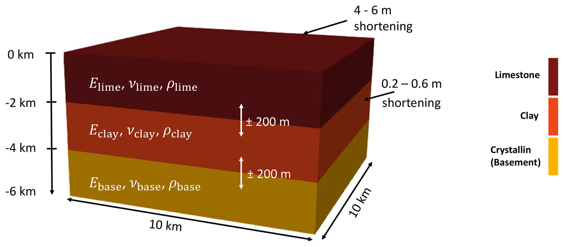
Figure 3 Schematic representation of synthetic model and all variations investigated in this study. The model ($\mathrm{10}\mathrm{km}\times \mathrm{10}\mathrm{km}\times \mathrm{6}\mathrm{km}$) consists of three different lithological units having purely elastic material properties, which are variable. Mechanical parameters are the Young modulus (E), the Poisson ratio (ν), and the density (ρ). The horizontal stratigraphic boundaries can be varied by ±200 m. The applied lateral boundary conditions range between 4 and 6 m shortening in the y direction driving S_Hmax magnitude and orientation and 0.2 to 0.6 m shortening driving the S_hmin magnitude and orientation.

For the different global SAs, we present first-order and total-order sensitivity indices. First-order indices describe the influence arising from the model parameters themselves, which are determined by the variance of the model parameter divided by the total variance that regards all model parameter variability. Total-order contributions contain the influence of the model parameters and their correlations to other parameters. For the sensitivity analysis, we need to define a threshold above which parameters are deemed influential. There is no general way of determining this threshold. For the purpose of this study, we set it to 10⁻² since values below this threshold would be difficult to validate against typical in situ stress measurement accuracies (Desroches et al., 2021; Martin, 2007; Morawietz et al., 2020). This value is also in accordance with threshold values typically employed in the literature (Cosenza et al., 2013; Degen et al., 2021a, b; Degen and Wellmann, 2024; Sin et al., 2011; Tang et al., 2007; Vanrolleghem et al., 2015). The threshold is a dimensionless number, which is determined by the division of two variances; for further details regarding the threshold itself and its determination, we refer to Degen and Wellmann (2024).

3 Synthetic model

We consider a three-layer model to investigate systematically the potential of the NI-RB method to construct reliable surrogate models for representing the subsurface stress distribution. The model has an extent of 10 km in both the x and y directions and 6 km in the z direction (Fig. 3). For the discretization, we consider hexahedral elements. In both the x and y directions, we have a model resolution of 400 m and in the z direction a resolution of 10 m. The much higher resolution of the vertical component is chosen to allow the consideration of geometrical uncertainties, i.e., uncertainties in the depth of geological horizons. The three layers are lateral homogenous and equally spaced, where the top layer consists of limestone, the middle layer is clay, and the lowest layer is a crystalline unit. Thus, S_v, S_Hmax, and S_hmin are indeed the principal stresses of the modeled total stress.

Throughout the study, we allow variations for the boundary conditions, the material properties, and the interface depths. For the displacement in the y direction (northern boundary), we apply a Dirichlet boundary condition with values varying between 4–6 m shortening, whereas the variations for the x direction range from 0.2 to 0.6 m (eastern boundary). Different boundary conditions are needed to ensure reasonable variations in the stress magnitudes as observed in data records. The top boundary is assigned with a zero Neumann boundary condition, and all remaining boundaries are subjected to zero Dirichlet boundary conditions normal to the boundary (roller boundary conditions). The material properties are varied according to the expected uncertainties for the corresponding lithology. The depth of geological horizons can be varied by ±200 m.

We consider five cases: (i) changing boundary conditions, (ii) changing material properties, (iii) changing interface positions, (iv) simultaneously changing boundary conditions and material properties, and (iv) changing all three sources of uncertainty. The different scenarios including their input parameters are listed in Table 1. The uncertainties of the parameters are chosen in a way comparable to those encountered in data sets or case studies (e.g., Bär et al., 2020; Bond et al., 2015; Ziegler and Heidbach, 2024).

4 Results

In the following, we present the construction of a geomechanical surrogate model. To understand the different requirements and impacts of the different sources of uncertainties, we first vary them individually and then investigate the combined effects. In order to validate the NI-RB results, for each test case randomly chosen parameters are used in several full-order model runs which are then compared to the NI-RB results.

4.1 Case 1: changing boundary conditions

We first investigate the potential of using surrogate models to determine the influence of uncertainties in the stress magnitude data records that are available. This is achieved by changing the displacement boundary conditions in a way that corresponds to uncertainties in the stress magnitude data. Therefore, we use the model displayed in Fig. 3 and construct a training set of 100 simulations, where we allow a variation in the boundary condition but keep all the material properties and the interface positions fixed.

Since we only vary the Dirichlet boundary conditions along the x and y axes, we evaluate the surrogates only for the horizontal components of the stress tensor, which are displayed in Fig. 4a and b. We observe that both the S_hmin and S_Hmax contributions of the stress tensor are represented by the surrogate model well. The global model errors for the scaled training and validation data set are for the S_hmin component of the order of 10⁻¹⁵ (about 10⁻¹² MPa²) and for the S_Hmax component of the order of 10⁻⁸ (about 10⁻⁴ MPa²), which means that visually no difference between the full and reduced solutions is detectable (Fig. 4). To calculate the global model errors, we use the mean squared error (MSE):

$$\begin{array}{}\text{(7)}& {\displaystyle }{\displaystyle }\text{MSE}(u_{\text{fe}},u_{\text{rb}})={\displaystyle \frac{\mathrm{1}}{N}}\sum _{i=\mathrm{0}}^{N-\mathrm{1}}{\left(u_{\text{fe}}-u_{\text{rb}}\right)}^{\mathrm{2}},\end{array}$$

where u_fe refers to the finite element solution.

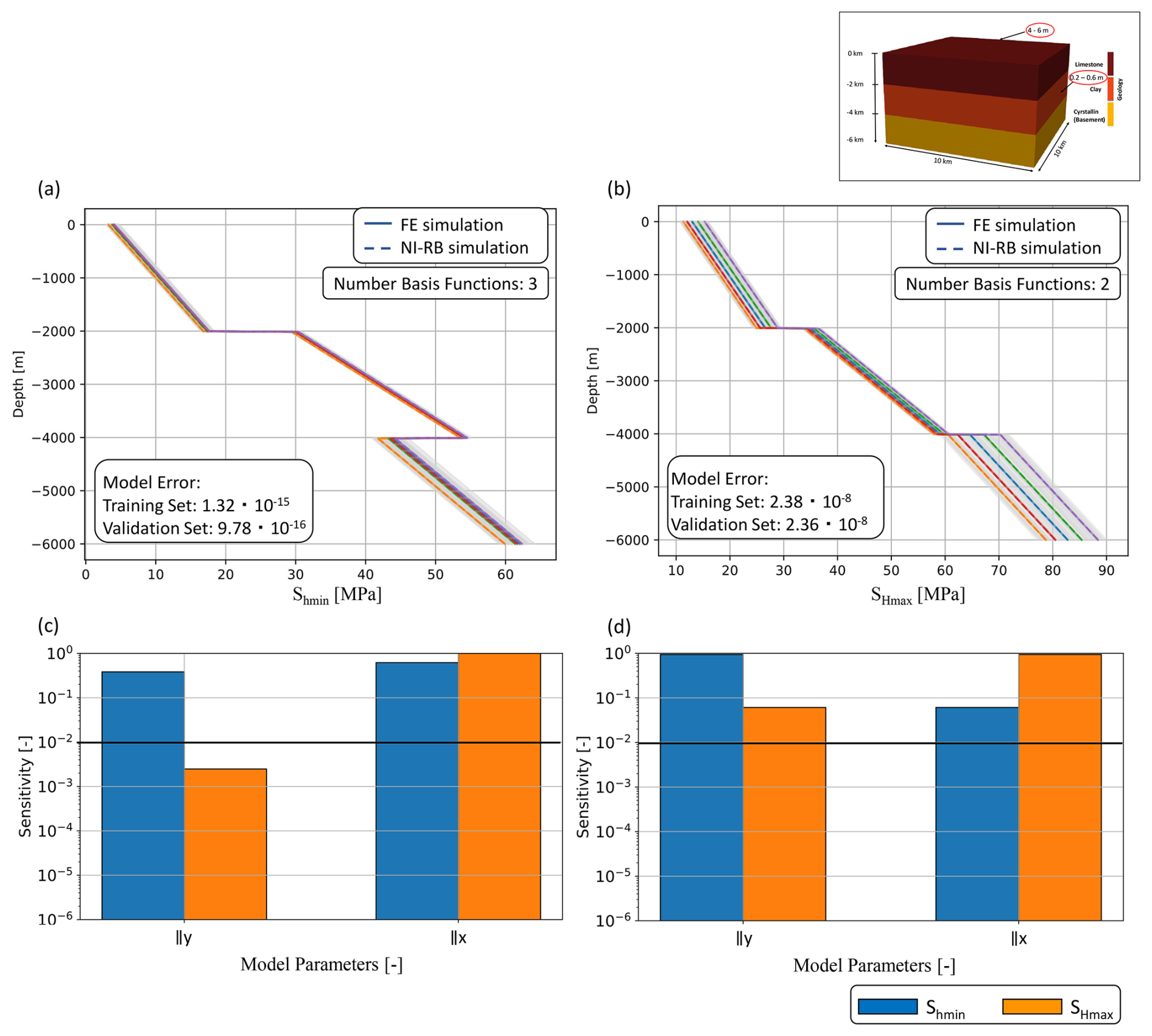
Figure 4 Investigation of the potential of surrogate models to determine the influence of varying boundary conditions. Comparison of the surrogate model accuracy for five randomly chosen realizations of the validation data set for (a) the S_hmin and (b) the S_Hmax components of the stress tensor. Note that “Sensitivity” denotes the value of the sensitivity index (Sect. 2.4), and ∥x and ∥y denote displacements parallel to the xaxis and y axis, respectively. The full-order solutions are denoted by colored solid lines and the reduced solutions by colored dashed lines. The different colors represent the stress response for different boundary condition values. The training data set consisting of 100 samples is indicated with light gray lines. Furthermore, we show the global SA results for (c) non-equal x and y strains and (d) equal x and y strains.

The results for the surrogates are obtained with only a few basis functions: two and three for the S_Hmax and S_hmin contributions, respectively. This demonstrated a general low complexity induced by the changes in model parameters and serves as a good illustration of how the NI-RB method operates. In contrast to other machine learning techniques, the method does not try to learn the state behavior of the stress directly. Instead, it investigates the changes in the state distribution because of different model parameters. In this example, this change yields a simple shift in the response, where the amount of shift varies for the different geological layers. This is also the reason why the abrupt shift in stress magnitude at interfaces is perfectly captured in all reduced solutions since only the magnitude of the shift but not the position changes.

In general, we observe the highest variability in the stress response for the S_Hmax component. This is caused by the boundary conditions since we assigned higher displacement values parallel to the x axis than parallel to the y axis. The global SA, displayed in Fig. 4c and d, confirms these findings.

In Fig. 4c, we observe a significantly higher influence of the boundary condition applying a displacement parallel to the x axis for both stress components. In the case of the S_Hmax component the boundary condition along the y axis does not impact the response notably. To offer a final proof, we repeated the surrogate model construction and the sensitivity analysis, considering equal parameter ranges of 4–6 m for both boundaries. This analysis with equal parameter ranges is referred to as “equal strains”, whereas the original setup is denoted as “non-equal strains”. The results of the corresponding SA are seen in Fig. 4d. In comparison to the previous analysis, we obtain increasing influences of the boundary conditions along the y axis. This yields precisely mirrored behavior for the S_Hmax and S_hmin components.

4.2 Case 2: changing material properties

We now investigate the variation in material properties. In this geomechanical study, we consider the variations in the Young modulus, the Poisson ratio, and the density for each layer individually. This results in nine parameters that can change, whereas for the previous example of the boundary conditions, we only had two parameters. Therefore, we increase the size of the training data set from 100 to 200 full-order solutions to compensate for the expected increase in complexity.

Although we have an increase in the number of parameters that we consider, we still fit the full solution very well with the reduced order model. Note that we investigate the stress distribution for the S_hmin, S_Hmax, and S_v components, which are displayed in Fig. 5a to c. The S_hmin and S_Hmax contributions show similar behavior regarding the global errors, where we obtain errors of the order of 10⁻⁹ for the scaled validation set (corresponding to 10⁻⁵ MPa²) and up to 10⁻¹⁷ for the scaled training data set (corresponding to 10⁻¹⁴ MPa²). The global errors for the S_v component are of the order of 10⁻¹⁵ (about 10⁻¹⁰ MPa²) for both the scaled training and validation data sets. However, we observe an increase in the number of basis functions from two or three to six for the horizontal stress responses. This increase in the number of basis functions is caused by the increased complexity, which shows the general scaling behavior of the NI-RB method. The dimension of the surrogate model is scaling with the complexity induced by the variability in the parameters. But this does not mean that an increase in the number of variable parameters automatically yields reduced dimensions. Relevant for the dimension is the number of variable parameters that lead to a change in the model response, so in our case the stress distribution.

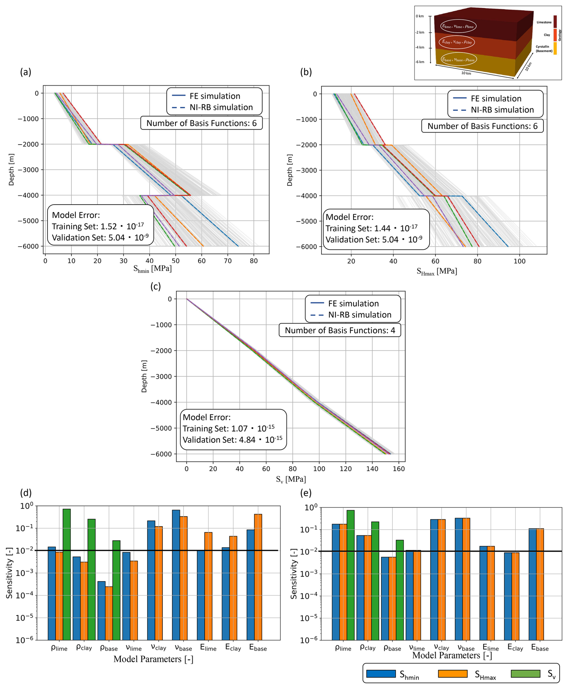
Figure 5 Investigation of the potential of surrogate models to determine the influence of varying material properties. Comparison of the surrogate model accuracy for five randomly chosen realizations of the validation data set for (a) the S_hmin, (b) the S_Hmax, and (c) the S_v components of the stress tensor. Note that “Sensitivity” denotes the value of the sensitivity index (Sect. 2.4). The full-order solutions are denoted by colored solid lines and the reduced solutions by colored dashed lines. The different colors represent the stress response for different material property values. The training data set consisting of 200 samples is indicated with light gray lines. Furthermore, we show the global SA results for (d) non-equal x and y strains and material parameter ranges and (e) equal x and y strains and material parameter ranges.

This is nicely demonstrated by comparing the number of basis functions of the S_hmin or S_Hmax contribution with the S_v component. For the vertical stress response, we only obtain four basis functions, which is the first indication that fewer parameters influence the stress response. This is later also confirmed by the SA. Still, six basis functions of the horizontal components are also a low number, taking into account that we vary nine parameters in total. So, as for the vertical component, this yields the assumption that not all parameters are influential with respect to the stress. As for the case of the changing boundary conditions, we obtain the highest variability for the S_Hmax component of the stress distribution. This is again caused by the higher boundary value of the displacement parallel to the x axis. The results regarding the variability in both the stress distribution and the number of basis functions are confirmed by the sensitivity analysis, which we present in the following.

The results of the SA are shown in Fig. 5d and e. Here, we investigate again two possible scenarios. The first scenario chooses the variation range of the material properties depending on the typically physically plausible variation range (Fig. 5d). This has the consequence that certain parameters have a wider relative variation range than others. To recover the underlying process behavior, we conduct the same analysis with a variation range of 3 % for all parameters and a displacement value of 5 m for both boundaries (Fig. 5e).

Focusing first on the results of the SA in Fig. 5d for the S_Hmax component of the stress (orange bars), we obtain the highest influences for the Young modulus of the crystalline layer, as it is the stiffest unit. This is followed by the Poisson ratios of the crystalline and clay layers and then by the Young moduli of the limestone and clay layers. All other model parameters are non-influential. Consequently, we have a high impact of the Young modulus and Poisson ratio but no influence of the density. This low influence is the cause of the in relation much lower variation range of the density. Assuming equal variation ranges for all model parameters, as seen in Fig. 5e, we obtain the increased influence of the density especially for the limestone and clay layers. At the same time, we retrieve decreasing importance for the Young modulus such that the density is ranked in between the Poisson ratio and the Young modulus.

Continuing with the S_hmin component (blue bars in Fig. 5d), we observe a higher influence of the Poisson ratios and a significantly decreased impact of the Young moduli in contrast to the S_Hmax component. The reason is again the different boundary values for the displacement. The differences between the two horizontal stress responses nearly vanish for the analysis with equal boundary conditions (Fig. 5e).

For the S_v component, we obtain in both scenarios only influences of the density, which demonstrates that the vertical stress component is predominantly driven by gravity, which corresponds to the definition. Furthermore, we have increasing influences of the density with decreasing depth values. Hence, we get the highest influence for the limestone layer, followed by the clay and crystalline layers, which is in agreement with a previous model study (Ziegler, 2022).

4.3 Case 3: changing geometry

For the scenario of a changing geometry, we consider two parameters, which are the interface depths between the limestone and clay layer (denoted as upper interface) and the interface between the clay and crystalline layer (denoted as lower interface). The upper interface is by default at a depth of 2 km, and the lower interface is at a depth of 4 km. For both interfaces a variation range of ±200 m is considered. As before, the training data set is constructed using a Latin hypercube sampling, but for the geometry, we have a training data set size of again 200 full-order solutions instead of the initial 100 due to the expected higher complexity compared to Case 1.

In addition to a higher complexity comparable to Case 2 a change in interface depths means that the geometry of the model is changed, which is different from the material properties or boundary condition changes. The challenges for the surrogate modeling approach become apparent from Fig. 6a. The surrogate model behaves differently in approximating the stress tensor compared to the previous two cases. The stress components (S_hmin component visualized in Fig. 6) are approximated well within the three layers such that again no visible differences are notable. However, at the transition between layers, the approximation quality is significantly decreased (marked with black ellipses). So, the surrogate has major issues resolving the position of the stress shift due to the changes in geological horizon depth. The difference to the previous examples is that the shift is no longer stationary and the number of elements per unit changes. In the case of changing boundary conditions and material properties, only the magnitude of the shift changes. But for the geometrical parameters, the magnitude stays roughly the same but the position of the shift can vary by ±200 m.

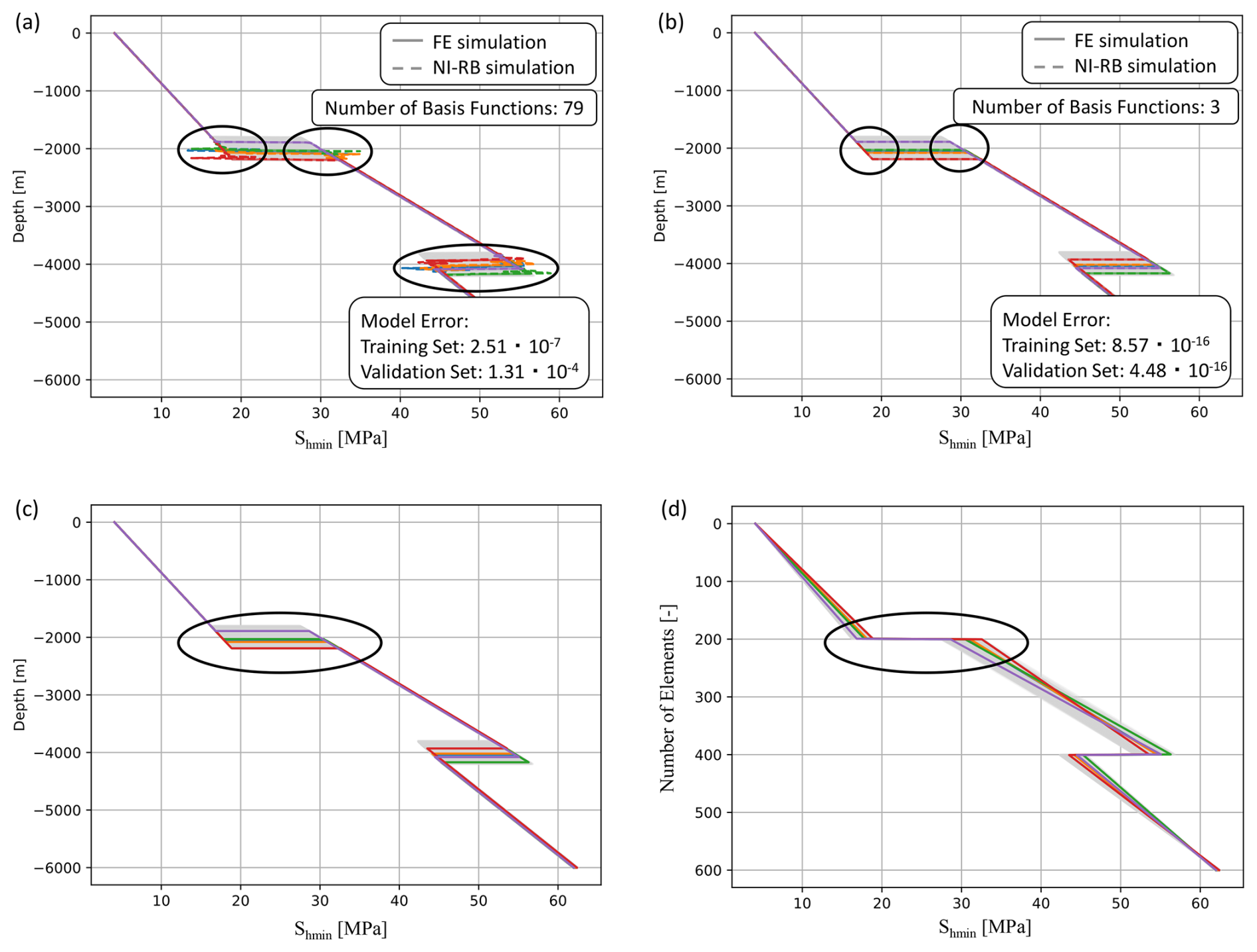
Figure 6 Challenge of accurately predicting the solution because of varying geometrical parameters. Comparison of the surrogate model accuracy for five randomly chosen realizations of the validation data set for the S_hmin component of the stress tensor for (a) the Gmsh model with a varying number of elements per layer and (b) the Gmsh model with a fixed number of elements per layer. Furthermore, we display a few realizations from the validation data set over (c) the depth and (d) the number of elements of the mesh.

To overcome this issue, the number of elements needs to remain the same for each lithology. This is achieved using Gmsh (Geuzaine and Remacle, 2009) for discretization, which allows for a higher flexibility during the construction of the structured meshes. Most importantly it allows for a fixed number of elements per lithology too, which is in our case 200. That means that the maximum vertical length of each element is 10 m but that also elements with smaller vertical length are produced depending on the interface location. This results in a better quality at the interface (Fig. 6b).

These two representations of the geometry result in the same depth vs. stress relationship (Fig. 6c), but for the surrogate model construction, we provide the information about the relationship of the number of elements vs. the stress distribution (Fig. 6d). This relationship is different for the two scenarios. For scenario 1 (Fig. 6a), we obtain the changing position of the shift. However, for scenario 2 (Fig. 6b), we have the shift again stationary since we always have 200 elements per subdomain independent of the interface positions. Consequently, the challenge associated with the geometrical characterization can be addressed by reformulating the original problem.

The difference in behavior is also clearly visible in the number of basis functions required to approximate the solution. We obtain 79 basis functions for the S_hmin component of the stress tensor, whereas the version with a fixed number of elements per subdomain only requires three basis functions. This means that we obtain 25 times more basis functions for the version with a changing number of elements per subdomain. Since the scaling behavior of the reduced model is tied to the complexity of the parameter space and not to the number of changing parameters, this demonstrates the change in complexity between the two model versions.

We now move to demonstrate the physical effects of changing the geometry, as presented in Fig. 7a–c. Regarding the horizontal component, we obtain no difference within the layer, which is in accordance with our expectations since neither the material properties nor the boundary condition values are changed throughout the simulations. Differences occur at the interface positions, which vary from realization to realization. Consequently, the transition in the stress values between one unit to the other is changing depending on the corresponding interface depth. Furthermore, we observe as in the previous example nearly no variations in the vertical component.

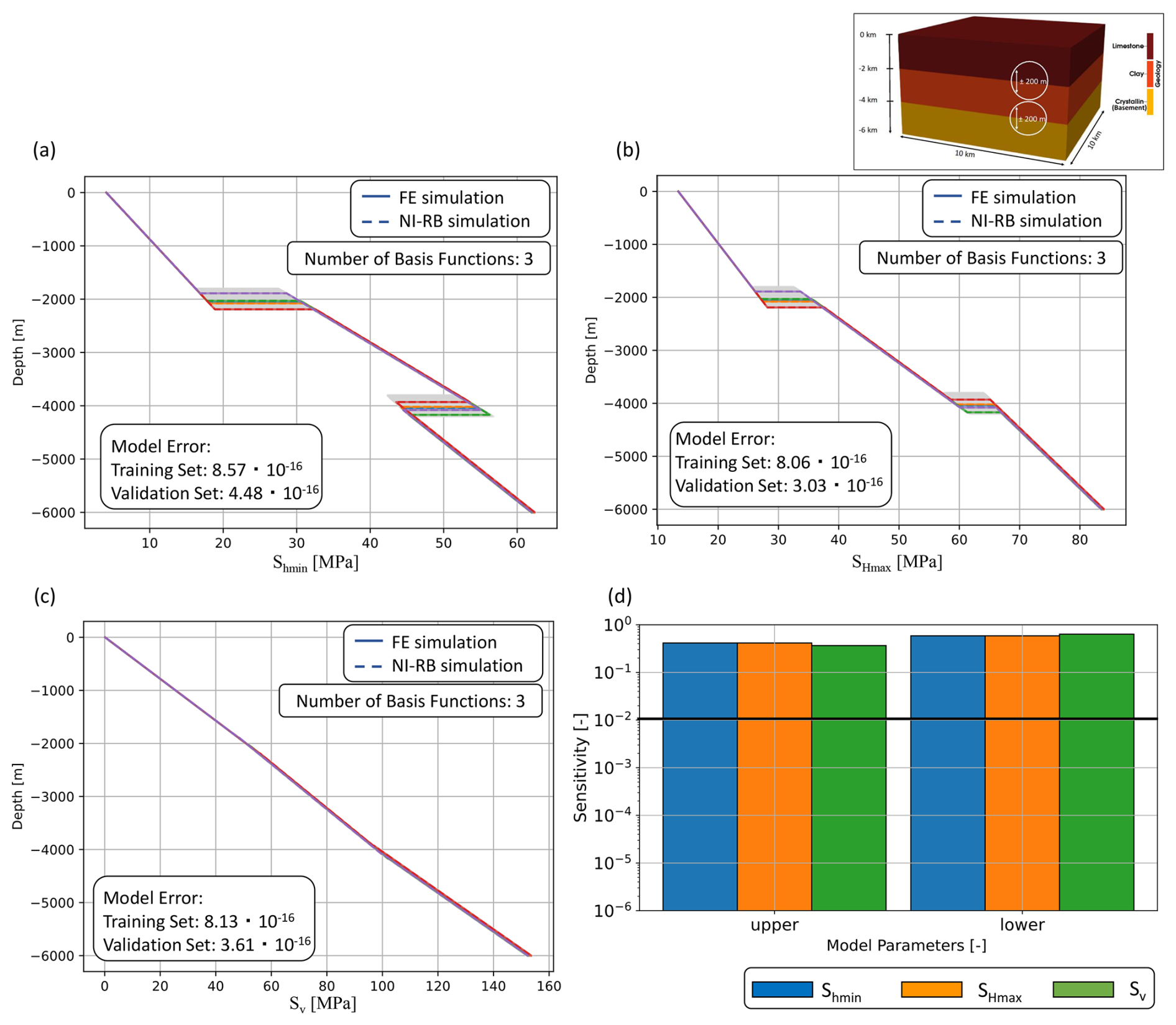
Figure 7 Investigation of the potential of surrogate models to determine the influence of varying interface depths. Comparison of the surrogate model accuracy for (a) the S_hmin, (b) the S_Hmax, and (c) the S_v components of the stress tensor. Note that “Sensitivity” denotes the value of the sensitivity index (Sect. 2.4). The full-order solutions are denoted by colored solid lines and the reduced solutions by colored dashed lines. The different colors represent the stress response for different interface depths. The training data set is indicated with light gray lines. Furthermore, we show in (d) the global SA results.

Regarding, the sensitivity analysis (Fig. 7c), we observe identical behavior for changes in both interface depths for the horizontal stress tensor components. For the vertical contribution, we observe a slightly higher influence of the location of the lower interface on the stress response. This higher influence is caused by the higher-density contrast of the clay and crystalline layer with respect to the limestone and clay layers. Note that the lack of parameter correlations observable throughout all three scenarios is induced by the linearity of the application; this image significantly changes once nonlinear problems are considered.

4.4 Case 4: simultaneously changing boundary conditions and material properties

In the previous three scenarios (Case 1–3), we investigated the behavior of the surrogate model individually for the three sources of variability considered in this paper. However, in a real-case application, it is unlikely that only one source of uncertainty is present. Typically all sources of uncertainty occur and can differ in their degree of variability. To evaluate which consequences this poses in terms of the surrogate, we consider two additional cases. In this section, we account for a simultaneous variation in both the boundary conditions and the material properties. The case of varying all three sources of uncertainty at the same time is presented in the next section.

Analyzing the combined effect of varying the boundary condition and the material properties is of interest for two main reasons: (i) does it yield an increase in complexity and consequently an increase in the dimension of the surrogate and (ii) how is the SA affected by the increase in variable parameters?

Starting with the first aspect of complexity, we obtain for all three components of the stress tensor the same number of basis functions (Fig. 8a–c) as for the case of changing only the material properties (Case 2). So considering additionally the boundary conditions next to the material properties does not increase the complexity notably. This might seem counter-intuitive at first glance since we consider 2 additional parameters yielding a total number of 11 parameters. The reason for this behavior is two-fold: (i) the simplicity of the geological model, and (ii) the threshold behavior of the POD. We use a relatively simple benchmark with horizontal horizons to enable a better understanding of the surrogate construction method. However, this also means that the model has an underlying less complex behavior which is mirrored in the low number of basis functions obtained. For more complex models at least a slight increase in the number of basis functions is expected if the additional parameters influence the model response. That this is the case, we see later on in the SA. The second aspect is about the POD threshold. We defined an error tolerance of 10⁻⁴ % for the POD. This means that the POD can disregard at most 10⁻⁴ % of information content. So, it could happen that for the less complex scenario, the error decreases with the addition of the sixth basis function to 10⁻⁵ %, whereas it decreases only to $\mathrm{2}\times {\mathrm{10}}^{-\mathrm{4}}$ % for the more complex scenario. In that case, both scenarios would have the same number of basis functions, although the complexity impacts the accuracy of the model. Note that this is not occurring in our example. Both the scenario of changing material properties and the scenario of varying material and boundary conditions have comparable accuracies. This means that here, the complexity is not increased by considering in addition to the material properties also the boundary conditions. However, this is caused by the simplicity of the model and will not occur for more complex studies. The reduced solution captures the full-order response well for all three stress tensor components, and we retrieve similar global errors in the case of changing only the material properties.

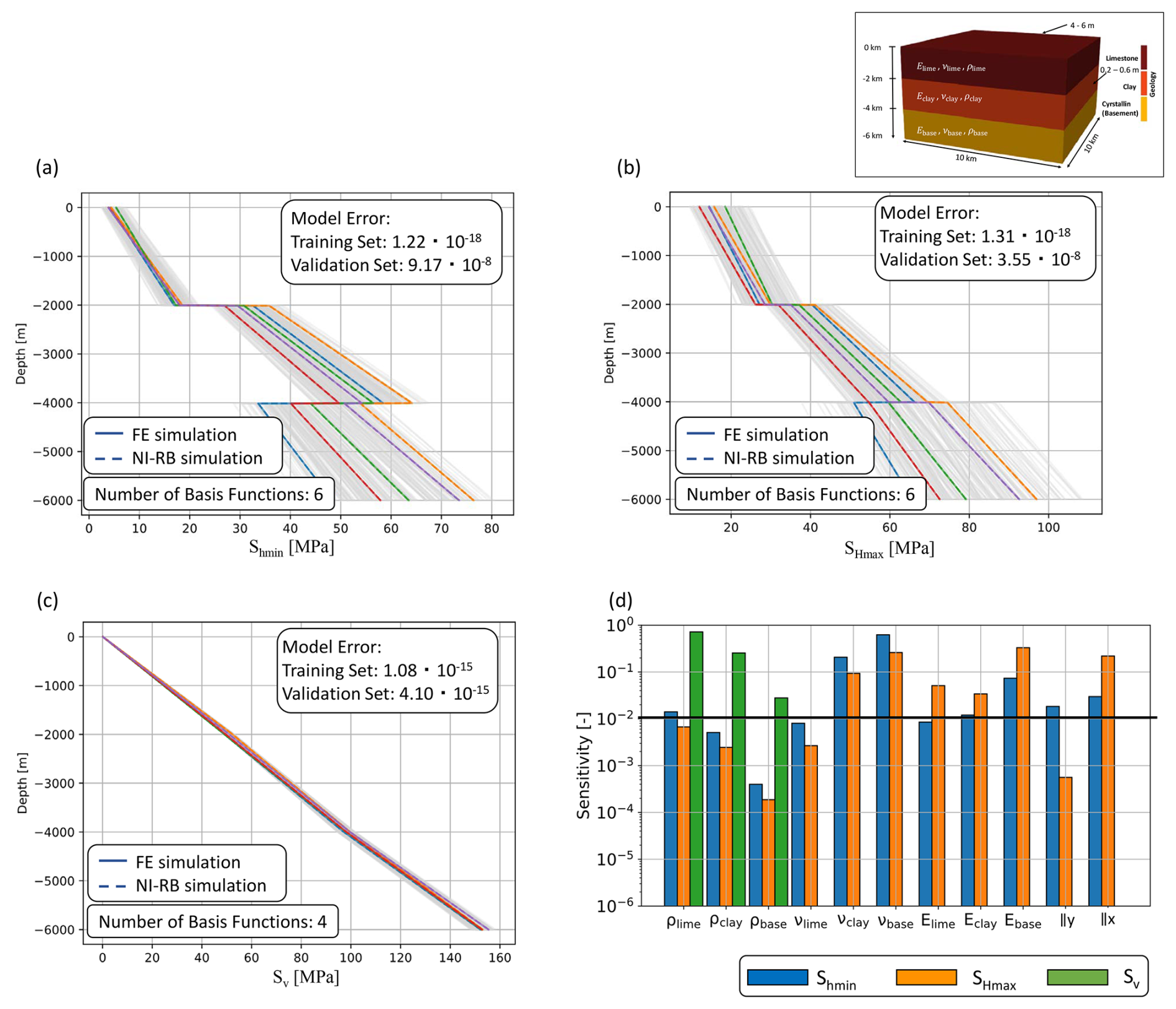
Figure 8 Investigation of the potential of surrogate models to determine the influence of varying boundary conditions and material properties. Comparison of the surrogate model accuracy for five randomly chosen realizations of the validation data set for (a) the S_hmin, (b) the S_Hmax, and (c) the S_v components of the stress tensor. Note that “Sensitivity” denotes the value of the sensitivity index (Sect. 2.4). The full-order solutions are denoted by colored solid lines and the reduced solutions by colored dashed lines. The different colors represent the stress response for different boundary conditions and material properties. The training data set consisting of 200 samples is indicated with light gray lines. Furthermore, we show in (d) the global SA results.

Switching focus to the sensitivity analysis (Fig. 8d), we see no correlations between the boundary values and the different material properties. This is expected since we consider a linear physical process. This would in general justify a separate consideration of the two sources of uncertainties. Still, a joint consideration has several advantages. The first benefit concerns generalizability. Only for linear applications are no correlations expected; for nonlinear problems correlations are likely to occur. So, introducing the joint approach allows for a straightforward extension to nonlinear applications. Furthermore, even for the linear case, the joint approach has the benefit of being able to determine which relative impact the boundary conditions have with regard to the different material properties.

This is seen in the SA results of Fig. 8d, where we obtain a very similar result to the analysis considering only material properties. However, we can now determine the rank of the boundary condition values with respect to the Young modulus, the Poisson ratio, and the density. The boundary condition along the x axis has a similar importance to the Young modulus of the crystalline layer for both horizontal components of the stress tensor. The same is true of the other boundary condition in the case of the S_Hmax component of the stress. For the S_hmin component the boundary condition along the y axis is non-influential with regard to the stress response. This matches the previously observed behavior of the scenarios changing only the boundary conditions or the material properties. The S_v component remains entirely gravity-driven, and hence no influence of changes in the boundary conditions is detectable.

4.5 Case 5: simultaneously changing boundary conditions, material properties, and geometry

Considering the case of simultaneously changing the boundary conditions (using the setup presented in Fig. 6b), material properties, and the depth of the interfaces, we first observe a slight increase in the number of basis functions compared to the case of only changing the geometry (Case 3) and the same number of basis functions as for the case of changing both the material properties and boundary conditions (Case 4). Also, the global errors are about 10⁻¹⁸ for the training data set and 10⁻⁷ for the validation data set for the horizontal components of the stress tensor of similar orders of magnitude to the previous case (Fig. 9a–c). Only the global error of the validation data set for the vertical stress component is at 10⁻¹² slightly increased because of the higher complexity of the response. This higher complexity arises from the combined influence of the density and interface position as shown in the SA (Fig. 9d).

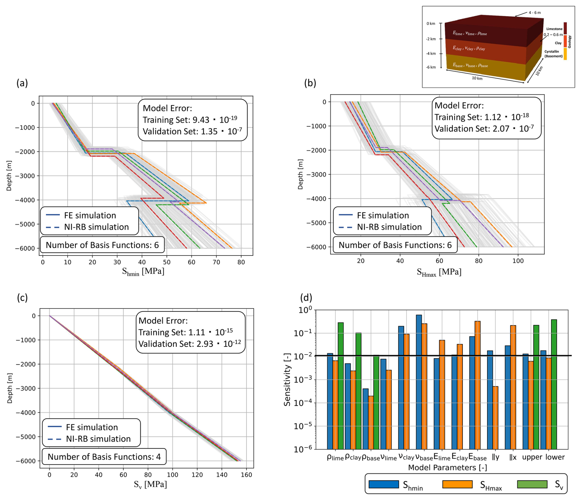
Figure 9 Investigation of the potential of surrogate models to determine the influence of varying boundary conditions, material properties, and the interface depths. The figure shows a comparison of the surrogate model accuracy for five randomly chosen realizations of the validation data set for (a) the S_hmin component, (b) the S_Hmax component, and (c) the S_v component of the stress tensor. Note that “Sensitivity” denotes the value of the sensitivity index (Sect. 2.4). The full-order solutions are denoted by colored solid lines and the reduced solutions by colored dashed lines. The different colors represent the stress response for different boundary conditions, material properties, and interface depths. The training data set consisting of 200 samples is indicated with light gray lines. Furthermore, we show in (d) the results of the global SA.

Furthermore, the SA demonstrates that for S_hmin, we obtain only minor influences of the interface positions, and for S_Hmax we obtain negligible impacts. So for the given variation ranges and model geometry, the material properties and boundary conditions have a higher impact than the geometrical parameters.

4.6 Case study – Nördlich Lägern

So far, we focused on a benchmark problem to better illustrate the concepts of surrogate modeling for geomechanical applications. To demonstrate that the methodology is also applicable to a more realistic setting, we extend our considerations to a model based on the lithological variability in a potential siting region for radioactive waste, Nördlich Lägern in northern Switzerland. The model is a simplified version of the model of Hergert et al. (2015) with the stratigraphy and their depth inspired by the well Stadel-3-1 (Crisci et al., 2022a). The model does not have any lateral variation in the topography or layer thickness, nor do the units have an inclination, as observed in that region. Therefore, we construct a model (Fig. 10) with an extent of $\mathrm{2500}\mathrm{m}\times \mathrm{2500}\mathrm{m}\times \mathrm{1400}\mathrm{m}$ with five elements in each horizontal direction (x and y directions) and 140 elements in the vertical direction for each of the 15 layers to ensure a vertical resolution of minimum 3 m. We on purpose use the same number of elements for each layer to avoid a bias in the sensitivity analysis caused by the layer thickness. To elaborate, consider a model consisting of two layers, where the top layer has a thickness of 500 m and the base layer has a thickness of 200 m. If we discretize the model with a vertical resolution of 100 m, we require five elements for the first layer and two elements for the second layer. Calculating the sensitivity indices takes the variation in the stress distribution in each element into consideration. Consequently, the top layer will have more elements contributing and, because of that, likely a higher impact. By discretizing the model with an equal number of elements per layer (e.g., five elements for both the top and base layer), we can avoid this effect. For further information regarding potential biases, we refer to Degen and Wellmann (2024). For this model, we consider only variations in the Young modulus. We do not consider the variability in the other elastic material properties since the density is well-known from density logs of boreholes, and both the density and the Poisson ratio demonstrated little impact in previous studies (e.g., Gölke and Coblentz, 1996; Reiter, 2021; Ziegler, 2022). All linear elastic input parameters are listed in Table 2. Regarding the boundary conditions, we follow a similar approach to the previous models. The eastern boundary has a Dirichlet boundary condition of 0.14 m extension, and the southern boundary has a Dirichlet boundary condition of 1.8 m shortening. The top boundary is associated with a zero Neumann boundary condition, and all other boundaries are subjected to zero Dirichlet boundary conditions normal to the boundary.

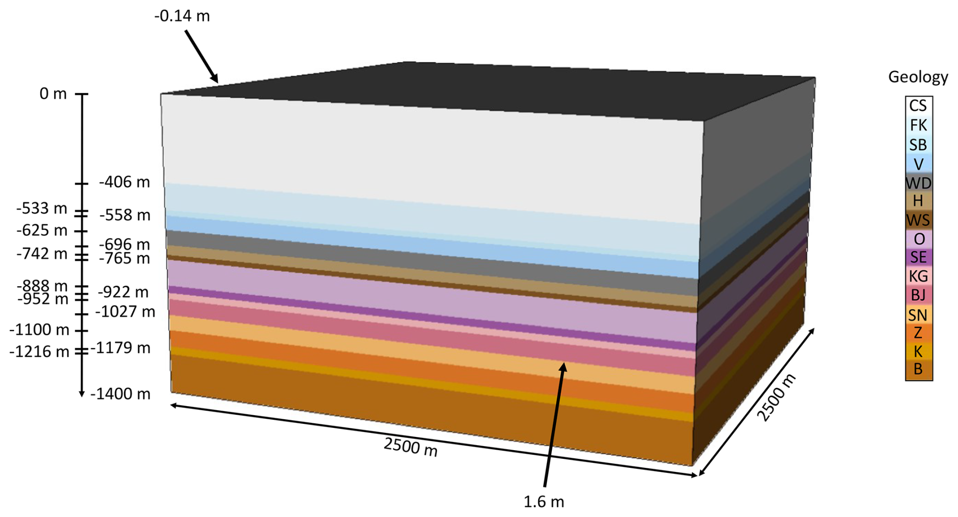
Figure 10 Schematic representation of the simplified model based on the well Stadel-3-1, representing the case study of Nördlich Lägern in Switzerland. The geomechanical units are the Cenozoic sediments (CS), Felsenkalke (FK), Schwarzbach Fm. (formation) (SB), Villigen Fm. (V), Wildegg Fm. (WD), Herrenwis Fm. (H), Wedelsandstein Fm. (WS), Opalinus clay (O), Staffelegg Fm. (SE), Klettgau Fm. (KG), Bänkerjoch Fm. (BJ), Schinznach Fm. (SN), Zeglingen Fm. (Z), Kaiseraugust Fm. (K), and the basement including Buntsandstein and Rotliegend (B). The lateral boundary conditions of the model are a shortening of 1.6 m from the south and an extension of 0.14 m in an eastern direction.

Table 2 Variation ranges of the Young modulus (E) and values for the other elastic material properties, as well as the layer thicknesses, for the case study of Nördlich Lägern. The parameter ranges are publicly available in the technical report by NAGRA (2024). Note that Fm. signifies formation. The data on the Young modules are based on information jointly inferred from four boreholes: Bachs-1-1, Bülach-1-1, Stadel-2-1, and Stadel-3-1 (Crisci et al., 2021, 2022a, b). The thickness data are derived from well Stadel-3-1 (Crisci et al., 2022a).

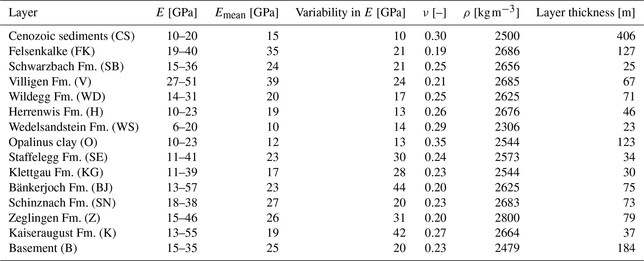
The stratigraphic column is inspired by the well Stadel-3-1, and the material properties are based on data from the four boreholes Bachs-1-1, Bülach-1-1, Stadel-2-1, and Stadel-3-1 that are presented in Dossiers VI and IX, which can be downloaded from NAGRA (download at https://nagra.ch/downloads, last access: 17 February 2025). These are in particular the NAGRA Working Reports NAB 22-04 (Bachs-1; Gonus et al., 2023), NAB 22-26 (Bülach-1; Spillmann et al., 2022), NAB 22-02 (Stadel-2; Crisci et al., 2022b; Gonus et al., 2022b), and NAB 22-01 (Stadel-3; Crisci et al., 2022a; Gonus et al., 2022a). Consequently, also the geometrical representation is subjected to low uncertainties, meaning that we do not vary the interface positions for this case study. Lastly, the boundary conditions are derived from a previous study by Hergert et al. (2015) and remain the same throughout all realizations.

As for the previous section, we first present the approximation quality and other characteristics of the surrogate models themselves. For the surrogate model of both the S_hmin (Fig. 11a) and S_Hmax components (Fig. 11b), we observe overall a similar approximation quality as for the benchmark study demonstrating the ability of the approach to be extended to more complex settings. The highest inaccuracies in the predictions are observed for realizations yielding maximum stress values.

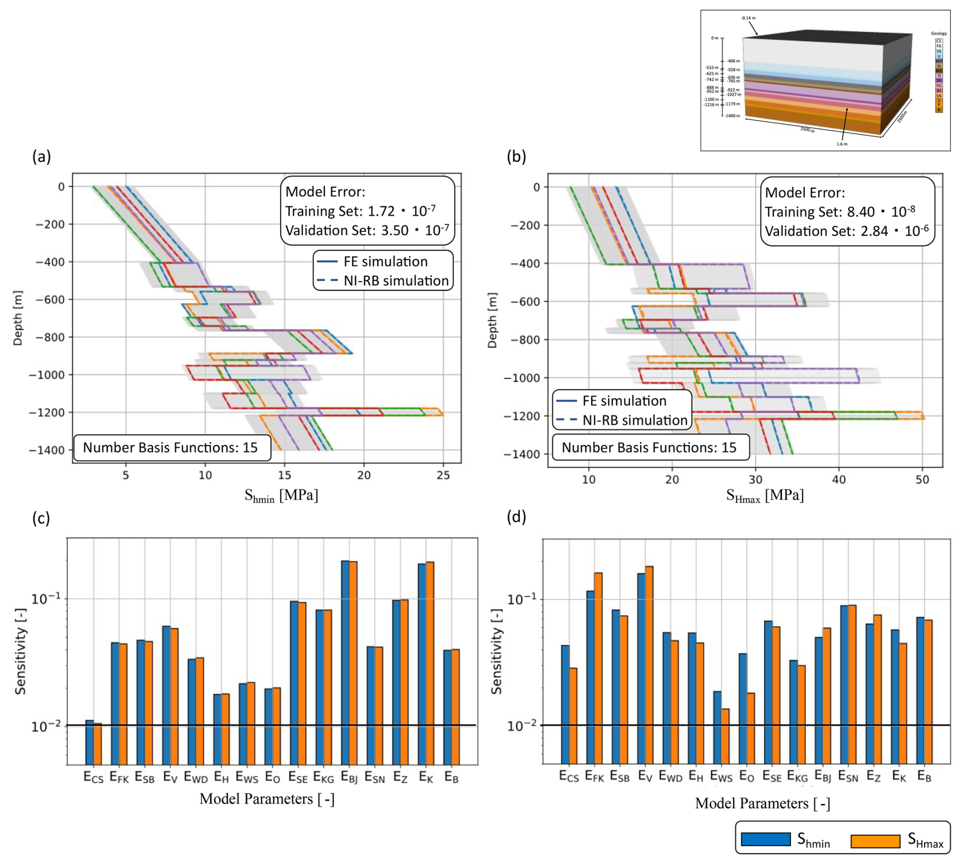
Figure 11 Investigation of the potential of surrogate models for the case study of Nördlich Lägern in Switzerland. Comparison of the surrogate model accuracy for five randomly chosen realizations of the validation data set for (a) the S_hmin and (b) the S_Hmax components of the stress tensor. Note that “Sensitivity” denotes the value of the sensitivity index (Sect. 2.4). The full-order solutions are denoted by colored solid lines and the reduced solutions by colored dashed lines. The different colors represent the stress response for different Young modulus values. The training data set consisting of 200 samples is indicated with light gray lines. Furthermore, we show the global SA results in (c) as non-equal and in (d) as equal parameter ranges.

Another interesting aspect is the number of basis functions, indicating the complexity of the parameter space. For both contributions of the stress tensor, we require 15 basis functions to achieve a POD tolerance of 10⁻⁴ %. Taking into account that we vary in total 15 Young modulus values, this demonstrates generally a low complexity of the models and holds promise for the extension to higher-dimensional parameter spaces. Note that we did not construct a surrogate model for the vertical stress component since we do not vary the density, and hence we obtain no variations in the vertical stress for all realizations.

Shifting to the results of the global SA, presented in Fig. 11c, we note that the Young modulus values of all 15 layers impact the responses of both horizontal stress components.

Consequently, for all of the following analyses, we would need to take all parameters into account. Although all parameters are deemed influential, we still observe differences in the amount of influence they have on the model response. For the S_hmin component, the Young modulus of the Bänkerjoch formation has the highest impact, followed by the Young modulus of the Kaiseraugust formation. Also, for the S_Hmax component these two formations yield the highest impact on the stress distribution, although their influences are reversed with respect to the S_hmin component. The main reason for the significant influence of these two layers is the large variation range in the Young modulus value. Another minor reason is the possible high contrast in the Young modulus to the adjacent layers partly because of this variation range. To better illustrate the impact of the variation range, the variability is shown in Table 2.

The significant influences of the Bänkerjoch and Kaiseraugust formations are followed by the significant influences of the Staffelegg, Klettgau, and Zeglingen formations. All three formations are characterized by variation ranges of about 30 GPa, so slightly lower variation ranges than the previously mentioned formations but higher variation ranges than for the units. This pattern is also observable for the remaining parameters within the global SA. So, within this global SA, the level of impact is mainly determined by the variation ranges of the Young modulus values. Consequently, the SA results are highly impacted by our prior knowledge since the different variation ranges are a result of heterogeneities or uncertainties within the layers. However, naturally, a wrong estimate of these parameter ranges yields a bias in the global SA. To investigate the potential differences in the SA, assuming similar heterogeneities and levels of knowledge for the individual layers, we repeated the SA with equal variation ranges for the Young moduli. Therefore, we used the mean values provided in Table 2 and applied variation of ±10 %. This yields a shift in the relevance of the different layers for the stress distributions. For both horizontal stress components, the Villigen formation has the highest impact, followed by the Felsenkalke and Schwarzbach formations. The lowest influences arise from the Wedelsandstein formation. Furthermore, low influences of the Opalinus clay are observed for the S_hmin component. Overall the influence of the individual layers in this configuration is mainly determined by the contrast in the Young modulus of the current layer and its adjacent layers.

5 Discussion

Within this study, we present how physics-based machine learning can be used to construct reliable surrogate models to predict the full stress tensor for a geomechanical model, e.g., for a nuclear waste disposal application. We start the discussion with general implications and challenges of surrogate modeling. Afterwards, we provide a comparison of physics-based vs. data-driven machine learning methods to emphasize the importance of appropriately choosing a surrogate model technique. Finally, we present application-specific aspects.

5.1 General implications and challenges for surrogate modeling

An important aspect is the explainability of the generated surrogate models. In the case of the NI-RB method, we perform first the POD which produces a number of basis functions. These basis functions are singular vectors characterizing the dominant physical behavior of the system. The machine learning part is only responsible for determining the weights of these basis functions. This has several implications. First, the non-provable part of the model and consequently the non-provable part of the error are solely restricted to the calculation of the reduced coefficients and are captured by a combination of scalar values. In addition, the errors that occur are explainable by considering both the physical relationship and the model geometry. As an example, in Fig. 11b, we observe very small visible deviations between the reduced and full-order models (e.g., for the orange lines at a depth of 1200 m). Still, these deviations occur in the form of shifts, yield smooth error distributions, and are not very pronounced. On the other hand, the errors in the neural network (NN) models (as we present in the next section) do not appear in the entirety of the model and introduce a noisy behavior in the error distribution. This means that they do not follow any physical relationship, which has been discussed in further detail in Degen et al. (2023).

In the literature (e.g., Degen et al., 2023; Faroughi et al., 2022; Raissi et al., 2019; Willard et al., 2022) physics-based machine learning is often used to reduce the amount of training data. The idea is that through introducing physical knowledge the number of admissible solutions can be decreased and hence less data would be required to train the surrogate models. Due to the simplicity of the presented example, this is a phenomenon that we do not observe. But note that this will become important for real-case studies.

In this paper, we investigate three sources of variability: (i) the boundary conditions, (ii) the material properties, and (iii) the geometry. As demonstrated the NI-RB method performs very well in constructing physically consistent surrogate models for considering variations in boundary conditions and material properties. The variability in the layer depth proves to be more challenging. This is especially pronounced for the presented linear elastic models since the high contrast in the material properties yields shifts in the stress distribution. However, this phenomenon occurs also for other applications, for instance, for hydrological studies, where the permeability contrast is large. So, this demonstrates the importance of reformulating the problem as presented in Sect. 4.3.

Reduced-basis methods using proper orthogonal decomposition and support vector machines (Zhao, 2021), recurrent neural networks (Kumar et al., 2021), or the empirical cubature method (Guo et al., 2024) as the projection method have already been used for mechanical applications, even considering the stress distribution. However, in the example presented in this paper, the high contrast in the linear elastic material properties (mainly Young's modulus but also Poisson's ratio and density) yields non-smooth distributions which result in consequences not discussed before. Furthermore, we also consider the variation in the geometrical parameters, which with the exception of Guo et al. (2024) have not been taken into account before. Note that Guo et al. (2024) consider geometrical variations for the context of two-scale simulations yielding very different requirements in terms of the stress conditions.

Another aspect we want to highlight is the global error. As seen for the case of changing geometrical parameters with changing number of elements per layer (Fig. 6a), the global errors are still low at 10⁻⁷ for the scaled training and 10⁻⁴ for the validation data set of the S_hmin component despite the inaccuracies at the interface location. This demonstrated the general problem of global error estimators. If there is a small region that has large deviations and the rest of the model regions are well fitted, this does not become apparent in the global error since this error considers an average over all realizations and the entire model domain. The other question is why the problem is more pronounced at the upper than the lower interface. Looking at the stress distributions, we see larger gaps between the different stress realizations at the upper interface than at the lower interface. Hence, in the case of the lower interface, better distributed information is available to determine the reduced solutions.

A major advantage of the RB method is the computational gain by using surrogate models instead of full-order model evaluations. Therefore, we briefly want to discuss the aspect of computational costs. The computational cost for all five scenarios is comparable with an execution time of about 3 min for a single finite element solution; in contrast, an evaluation of the surrogate required 0.1 ms, yielding a speed-up of 6 orders of magnitude. The speed-up does not consider the computational time during the offline stage. So, we want to extend the discussion by providing the computational cost for the construction of the surrogate. In this work, we used between 100–200 realizations for the training data set and up to 20 realizations for the validation data set. Hence, the most expensive surrogate model construction requires 220 realizations; with 3 min per realization this yields of cost of about 11 h. In addition to this cost comes the cost of performing the POD and the GPR, which are of the order of seconds. Since this is negligible with respect to the computational cost of constructing the data sets, we will discard this cost in the following. Consequently, the total construction cost of the surrogate model is equal to the cost of about 220 model evaluations. Comparing this to the over 50×10⁶ model evaluations required for the sensitivity analyses combined, the surrogate quickly pays off. It is also worth noting that the construction of the data sets is “embarrassingly” parallel, meaning that all model runs are completely independent. Therefore, parallel computing can be used to reduce the time. This is important because methods such as Markov chain Monte Carlo, used to quantify uncertainties, are not fully parallelizable. So, we not only save computation time but also shift the expensive computation to a stage where we can fully exploit parallel hardware infrastructures. This aspect, as well as how we can exploit graphics processing units, has already been discussed in detail (Degen et al., 2023). Another advantage is the non-intrusive nature of the algorithm, which allows for the straightforward inclusion of varying forward solvers.

The geometry considered in this study is simple: to focus on the surrogate model construction itself and its implications for geomechanical modeling. Both the non-intrusive and intrusive versions of the reduced-basis method have been applied to geothermal real-case studies with a complex geometrical setup, demonstrating a similar performance to that presented in this study (Degen and Cacace, 2021; Degen et al., 2021a, b, 2022a, b, c). This implies that especially for fixed geometries, no degradation in the surrogate model quality or performance is expected. Also, considering variations for complex geometries is possible. However, one should keep in mind that the base assumption for the method is the existence of a low-dimensional parameter space. Hence, if too many geometrical parameters are varied at once, this assumption breaks down, and the approach will become inefficient. As mentioned before, the non-intrusive reduced-basis method has been developed in order to provide an efficient extension of the RB method for nonlinear applications (Hesthaven and Ubbiali, 2018). In contrast to this study, Degen et al. (2022a) consider fully coupled thermo-hydro-mechanical simulations, demonstrating that the current approach is also extendable to nonlinear and coupled relationships. The implications for nonlinear applications are further detailed in Degen et al. (2023) for different subsurface applications, including the highly nonlinear Richard's equations. The results of these studies demonstrate great promise also for nonlinear geomechanical applications, which is especially important when considering potential extensions to elasto-plasticity.

5.2 Physics-based vs. data-driven machine learning techniques

To illustrate the differences between the data-driven and the presented physics-based machine learning method, we constructed another surrogate model for the case of simultaneously changing boundary conditions and material properties (Case 4) using a NN. The results are shown in Fig. 12 and yield several observations. First, the global errors in both approaches differ by orders of magnitude for both the training and the validation data sets. For the training data set, we achieve an error of the order of 10⁻¹⁸ for the non-intrusive RB method and 10⁻⁶ for the NN. We set for the POD a tolerance of 10⁻⁴ %. Since we use the root mean square error for the evaluation of the surrogate, that means the NN approach is 2 orders of magnitude less accurate than originally desired. This behavior is – albeit not as extreme – also observable for the validation data set, where we have errors of the order of 10⁻⁷ for the NI-RB method and 10⁻⁶ for the NN.

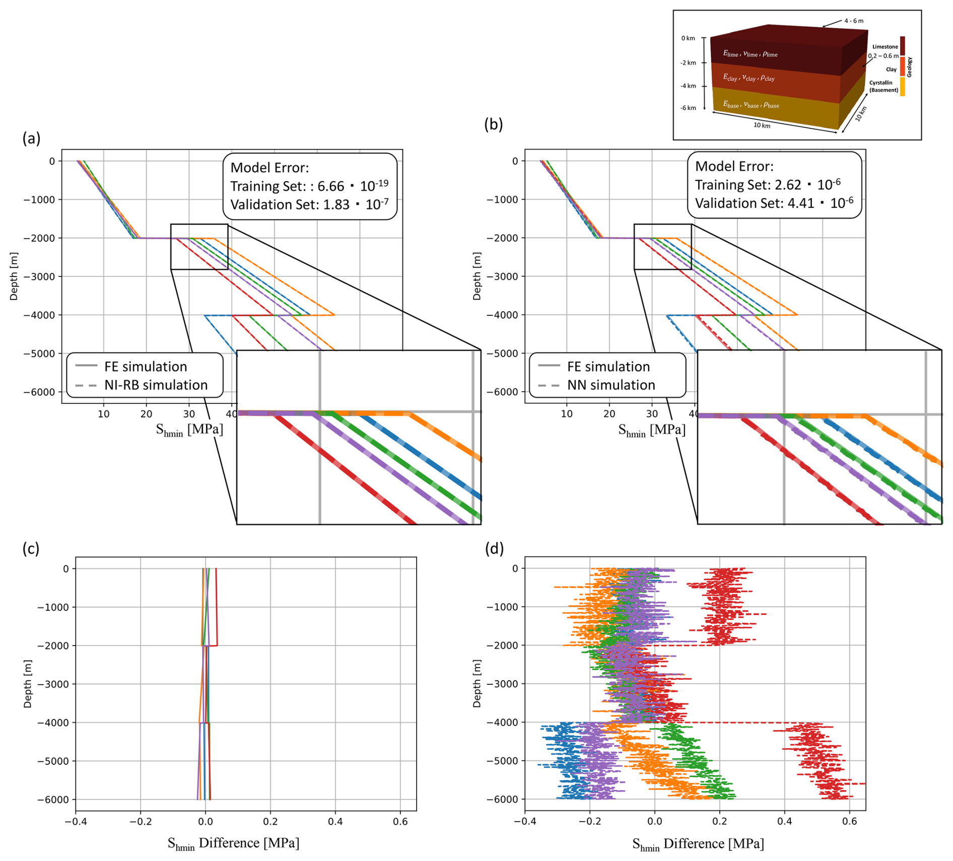
Figure 12 Comparison of the surrogate models constructed with (a) the non-intrusive RB method, (b) a neural network, (c) the difference between the non-intrusive RB solutions and the full-order solutions, and (d) the difference between the NN solutions and the full-order solutions for five randomly chosen realizations of the validation data set for the case of changing simultaneously the boundary conditions and material properties. The full-order solutions are denoted by colored solid lines and the reduced solutions by colored dashed lines. The different colors represent the stress response for different boundary conditions and material properties.

The difference in the error behavior is especially prominent when focusing not on the global errors but on the local distributions. Therefore, we plot in Fig. 12b the reduced solutions of the data-driven surrogate and the full solutions. At first glance, the approximation quality seems to be similar between the two surrogate models. However, by having a closer look major differences are observable. For the NI-RB surrogates the solutions are exactly on top of the full-order solutions, making them non-distinguishable by eye. In contrast, for the NN surrogate differences are directly visible. This can be best observed in the base layer for the red and blue lines. For the blue line, we obtain an underestimation of the stress response in the base layer, whereas for the red case the stress response is overestimated. This becomes more prominent by observing the differences between the full-order realizations and the NN solutions in Fig. 12d. But more interesting are the different overall responses of both surrogate models. The NI-RB reduced solutions are straight lines corresponding to the physical response. For the NN surrogate, we obtain mostly straight lines but with superimposed oscillations. To better highlight the differences, we plot in addition the differences between the non-intrusive RB and the full-order solutions in Fig. 12c and the differences between the NN and full-order solutions in Fig. 12d. The oscillations caused by the NN are not explainable from a physical perspective and are a result of treating the solutions in a purely data-driven manner within a statistical method. This demonstrates the fundamental difference between both approaches even without considering aspects such as the amount of available data. The NI-RB method produces solutions that follow the physical behavior, whereas the NN model produces results that statistically vary around this general physical response. In a presented trivial case, this does not matter. However, in more complex cases, these differences can be significant and crucial.

A comparison between the different physics-based machine learning methods, for instance, between the non-intrusive reduced-basis method and physics-informed neural networks (PINNs), is also interesting. In their original formulation, PINNs are designed for state estimation problems (Raissi et al., 2019). This makes a direct comparison of both approaches challenging since our study focuses on parameter estimation applications. Nonetheless, the error behavior of the PINN is expected to be similar to the one of the NN because of the architectural design of PINNs, as discussed in detail in Degen et al. (2023). A detailed comparison of the NI-RB method with other surrogate modeling approaches has been detailed in previous studies (Degen et al., 2023; Santoso et al., 2022), and since no conceptual changes are expected, they are not repeated in this study.

5.3 Implications for nuclear waste disposal applications

The subsurface stress distribution is of major importance in applications such as nuclear waste disposal, geothermal energy production, or subsurface (interim) storage of H₂ or CO₂. For these applications not only the cost of the numerical simulations but also their trustworthiness are essential since predictions have to be made over long periods of time and – in particular in the case of nuclear waste storage – false predictions can have major environmental impacts. The sparsity and uncertainty of available stress magnitude data, geological structures, and rock properties are a major challenge for the in situ stress prediction (e.g., Hergert et al., 2015; Morawietz et al., 2020; Ziegler and Heidbach, 2020). The uncertainties in the in situ stress state will then be transmitted to the results of forward models that predict the evolution of the stress state during, e.g., the excavation stage of the repository. In particular, long-term subsurface usage such as nuclear waste storage has to account for a broad range of different future scenarios which in turn drive the uncertainties. Therefore, the uncertainties of the initial stress prediction should be as small as possible.

We demonstrated the possibility of extending the methodology to more complex settings through the case study of Nördlich Lägern. An interesting aspect of the global SAs for this case study is the relative low impact of the Opalinus clay for the S_Hmax component, which is the target horizon for the future nuclear waste disposal site. This low impact means that within the tested variation ranges, changes in the Young modulus of the Opalinus clay do impact the maximum stress contribution less than most other layers. The largest impact arises from the stiff units. This is an important finding since it provides information about the impact of uncertainties on the planning phase of the nuclear waste disposal site. In the current study, we focus on the conceptual analyses of dominant physical processes and parameters in the form of sensitivity analyses. We do not consider real data on the stress magnitudes originating, for instance, from downhole measurements. This presents an interesting extension for future studies, where these measurements can be incorporated in the form of probabilistic uncertainty quantification methods, such as Markov chain Monte Carlo. This is interesting because many current studies consider best-case and worst-case scenarios only. A probabilistic uncertainty quantification approach allows not only the most likely scenario to be provided but also the associated range of uncertainties and their probability of being encountered. This is important for the planning of nuclear waste disposal sites since best- and worst-case analyses tend to estimate extreme values that have a low probability of being encountered. With a revised estimate of the uncertainties, the planning and construction might be improved, for instance, in terms of resource usage. Other potential future extensions include the incorporation of both global sensitivity analyses and uncertainty quantification into decision-making processes.

The last aspect we want to discuss concerns the sensitivity analysis. We investigate two scenarios, sensitivity analysis using (i) non-equal parameter ranges and (ii) equal parameter ranges. To understand why these different analyses were conducted it is important to note that as with every model, sensitivity analyses are designed with a specific purpose in mind. This purpose is defined in the quantity of interest and means that an SA is not easily reusable if the scientific question changes. In a typical application, we are interested in which model parameters impact the responses the most, so in our case, whether the Young modulus, the Poisson ratio, or the density has the highest impact on the stress distribution. In a realistic case study, the relative variation ranges of these various material properties may differ. That is the case because some properties can be determined with greater accuracy than others and properties such as the density have lower physically plausible variation ranges than, for instance, the Young modulus. This is a naturally occurring phenomenon, and we want to incorporate these into the SA. Therefore, typically the possible variation ranges are determined with respect to this prior knowledge yielding an SA with unequal parameter ranges.

Still, we are not always aiming to perform an SA to explain the behavior of a specific test site. In some cases, we are interested in what physical processes are driving the system. In this case, we would like to change the setup of the SA. To understand the driving forces independent of a specific site it might be beneficial to consider equal parameter ranges. This removes the bias that is introduced by the unequal parameter distributions. However, note that in most cases this bias is desired since it reflects the effects encountered in nature.

6 Conclusions

To conclude, we presented a physics-based machine learning model that can efficiently construct trustworthy surrogate models. The non-intrusive RB method enables evaluations that take less than a millisecond, whereas the full-order solves are in the range of minutes. This yields a speed-up of 6 orders of magnitude, demonstrating the use of these surrogate models for probabilistic uncertainty quantification, global sensitivity analysis, and parameter estimation studies in general.

In contrast to data-driven surrogates, the model follows the physical relationship and is physically explainable. This is of great importance for predictions and decision-making processes, as demonstrated in the highly sensitive case of nuclear waste disposal.

The surrogate models allow a simultaneous evaluation of both the boundary conditions and the material properties without losing relevant precision with respect to the full-order solutions. In addition, the incorporation of geometrical variations is possible without degrading the quality of the surrogate model. Therefore, this work lays the foundation for a joint consideration of all three sources of uncertainty for robust stress predictions.