TCSEIS-1D: An Interactive 1D Code for temperature and composition modelling of the crust and mantle from seismological data

We present TCSEIS-1D, a software to model the Earth's thermochemical and geophysical structure from the surface down to the core-mantle boundary (CMB). The code is designed to estimate geophysical parameters of the Earth's crust and mantle from petrological and thermal information within a thermodynamically consistent framework and to perform forward 1D coupled geophysical-petrological modelling of the structure of the Earth. Developed in Julia Language, the open-source code is intended to be an easy-to-use, flexible, and fast. TCSEIS-1D includes tools to exploit the large repertoire of 1D seismological data available, namely: surface wave dispersion curves (of fundamental and higher modes of Rayleigh and Love waves) and receiver functions (of P, S, and SKS waves). Surface heat flow and isostatic topography can also be modelled. Four simple examples that illustrate the capabilities of the code are presented to show the sensitivity of Rayleigh wave phase velocity curves and P-to-S receiver functions to compositional and temperature variations.

1 Introduction

The interpretation of geophysical data is a complex process that involves the quantitative treatment of measurements in order to retrieve information (presented as models or images) describing the Earth's inner structure (e.g., Aki et al., 1977; Dziewonski and Anderson, 1981; Telford et al., 1990; Grand, 2002; Rawlinson and Sambridge, 2003; Shapiro et al., 2005; Schaeffer and Lebedev, 2013; Fullea et al., 2021). The complexity and reliability of any geophysical model depend extensively on the nature (and quality) of the data selected for its characterization (e.g., Mosegaard and Tarantola, 1995; Bosch, 1999). For example, single-station P-to-S receiver functions analysis can be used to infer the depth of the Moho discontinuity and the average $V_{\mathrm{p}}/V_{\mathrm{s}}$ relationship for all the crust (e.g., Zhu and Kanamori, 2000; Niu and James, 2002), while surface wave dispersion measurements are suitable to image the shear-wave velocity structure of a region via inversion (e.g., Brune and Dorman, 1963; Yanovskaya et al., 1998; Priestley and McKenzie, 2006; Lebedev et al., 2009). Each one of these examples is largely limited by the sensitivity, resolution, and noise inherent to every individual data type. Receiver functions are sensitive to the depth of sharp acoustic interfaces (but can only resolve velocity contrast and not absolute velocities), whereas surface waves are sensitive to shear wave velocity gradients (with comparatively smaller sensitivity to interfaces, e.g., Julià et al., 2000). In order to overcome their individual limitations, both receiver functions and surface waves can be jointly inverted or modeled to study the lithospheric structure under a single seismological station (e.g., Julià et al., 2000; Tkalčić et al., 2015; Calò et al., 2016; Levin et al., 2023).

The integration of different data sets generally requires relationships between all the quantitative variables (physical properties) involved in the various forward problems. On the one hand, some of them can be relatively easily connected, like crustal compressional wave velocity (V_p) and density (ρ), for which several empirical formulas exist based on extensive databases (e.g., Ludwig et al., 1970; Christensen and Mooney, 1995; Godfrey et al., 1997; Brocher, 2005). On the other hand, other parameters like attenuation (Q_p, Q_s) or the relationship between shear wave velocity (V_s) and density (ρ) are comparatively more difficult to correlate. Although it is tempting to assume that all properties can be correlated by simple equations (e.g. a simple polynomial formulation cf. Bosch, 1999) or that some may be discarded (e.g., the assumption of elastic wave propagation), the reality is that it is more accurate to describe them with a probability density function within an integrated framework.

One effective approach to overcoming this issue is to estimate the required parameters directly from the petrological composition and the in-situ temperature and pressure conditions. For instance, density (ρ) and wave speeds (V_p and V_s) can be estimated from the rock's composition (𝒞), temperature (𝒯) and pressure (𝒫). Furthermore, as porosity and fluids can have a strong effect on these values at upper crustal levels corrections must be applied (e.g., Athy, 1930). Therefore, instead of trying to “guess” what an appropriate value for one master property would be, and then compute all others in relation to it (e.g., Jacobsen and Svenningsen, 2008; Arnaiz-Rodríguez et al., 2021), it is more advantageous and consistent to estimate all parameters directly from the Temperature-Pressure-Rock Composition triad (𝒯𝒫𝒞). In this way, we turn the “plural geophysical data” problem into the “lithology estimation” one, as named by Bosch (1999). The integrated geophysical-petrological strategy, as shown by many previous works (e.g., Afonso et al., 2008; Fullea et al., 2009; Khan et al., 2009; Munch et al., 2018; Bissig et al., 2021; Munch et al., 2021; Fullea et al., 2021), yields thermochemical results more straightforwardly interpreted into geological terms than classical – purely geophysical – approaches. Here, we present TCSEIS-1D (Temperature and Composition SEIsmological-1D), a simple forward code to model the thermal and compositional structure of the crust and mantle down to the core-mantle boundary (CMB) primarily from seismological data, i.e., Rayleigh and Love dispersion curves (group and phase velocity curves) and several types of elastic and isotropic receiver functions (the standard P-to-S as well as S-to-P and SKS-to-P). Available codes implementing an integrated geophysical-petrological modelling approach (either forward modelling or inversion) are mostly restricted to the lithosphere/upper mantle and do not include a lithological parametrization of the crust (e.g., Afonso et al., 2008, 2013a, b; Fullea et al., 2009, 2021).

TCSEIS-1D is implemented in Julia Language (Bezanson et al., 2017) for diverse reasons: it is widely used in the scientific community, flexible, open source, efficient, and has cross-platform compatibility, among others. Although Julia is still considered the “new” scientific language, it is actively used in geodesy, geostatistics, and seismology (e.g., Jones et al., 2020; Xu et al., 2008; Zhu et al., 2022), and it is rapidly spreading across different disciplines (e.g., Dinari et al., 2019; Gao et al., 2020). Among its most notable features are: (i) fast execution time (generally approaching C or Fortran-like performance); (ii) dynamic typing, debugging, and syntax correction (much like Matlab or Python); (iii) interoperability (it makes it easy to integrate codes from C, Python, Fortran, R, Matlab, etc.); (iv) geared toward scientific computing; multiple dispatch (multiple methods in the same function for different input arguments); (v) powerful parallel computing and GPU capabilities.

TCSEIS-1D can be employed to: (a) test geophysical models in the 𝒯𝒫𝒞 model space; (b) estimate a possible solution to the composition and thermal structure of the Earth's main layers (limited by the resolution, quality, and sensitivity of the input data), (c) link velocities and density variations to 𝒯𝒫𝒞 variations. After introducing the equations and assumptions that drive TCSEIS-1D's engine, the general framework of the code is presented, as well as the validation (against other codes) of the different sections that make up the software package. Finally, a few examples are presented to showcase the functionality and applicability of TCSEIS-1D with a suggestion of additional work for future versions. A general flowchart of the current version of TCSEIS-1D is provided in Fig. 1.

Figure 1 Schematic workflow of the TCSEIS-1D algorithm. User-defined inputs include layer composition, thickness of compositional boundaries, temperature at the surface, LAB and CMB, surface-wave periods and number of modes, receiver-function source depth and epicentral distance, and radial anisotropy. The code iteratively solves the heat equation to obtain the temperature profile, from which pressure and density are computed and used to redistribute mantle composition until convergence is achieved. Thermodynamic properties are then used to calculate seismic velocities (V_p, V_s), density (ρ), and attenuation (Q_s). The final 1-D model is used to compute surface-wave dispersion curves and receiver functions, followed by visualization and output of all model results.

2 Methods and Considerations

Mechanical properties of rocks, specifically compressional wave-speed (V_p), shear wave-speed (V_s), and density (ρ), vary in a wide range. Even though there are some clear trends in their behaviour (e.g., sedimentary rocks tend to have lower density than igneous rocks; or mafic rocks have higher V_p than felsic rocks; e.g. Telford et al., 1990; Brocher, 2005), a large degree of overlap exists. For example, a crustal rock with V_p=6.05 km s⁻¹ can represent a very old and consolidated carbonatic rock (i.e., a dolomite) or a felsic rock rich in quartz (i.e., a greisen). The consideration of metamorphic rocks affected by, for example, metastability (i.e., departure from thermodynamic equilibrium) makes this statement even more complex, as these rocks tend to show properties different from those associated with their protoliths (e.g., Telford et al., 1990).

Seismic velocities and density of Earth's rocks depend on several parameters, namely: temperature, pressure, mineral composition, melt fraction, fluids, and, in the case of crustal rocks, porosity and pore fluids (e.g., Christensen and Mooney, 1995; Brocher, 2005). This complex mixture yields the perfect recipe for the overlap of geophysical parameter values for different rock types and geological settings as usually reported (e.g., Telford et al., 1990; Brocher, 2005). For our purpose of modeling geophysical data using petrological and thermal parameters, it is cardinal to reduce the number of free variables while keeping, at the same time, a flexible enough parameterization to represent the Earth's complexity. In this study, for the crust, we chose several ternary diagrams to classify igneous and sedimentary rocks based on mineralogical composition (Streckeisen, 1974; Le Bas and Streckeisen, 1991; Philpotts and Jay, 2009; Bissell et al., 2021). By contrast, in the mantle, we adopt two major oxides (Al₂O₃ and FeO) as independent variables and compute the other CFMAS oxides (CaO, FeO, MgO, Al₂O₃, and SiO₂) from statistical correlations based on global mantle xenoliths and peridotite massifs databases (e.g., Afonso et al., 2013a, b; Fullea et al., 2021).

2.1 The geotherm

In general, temperature increases with depth (z) within the Earth. Heat transport inside the Earth is mainly a 3D problem in which the mantle is in convection at a high Rayleigh number (Ra>10⁷; e.g., Ricard, 1993), bringing heat from the Core-Mantle Boundary, where the D” layer acts as the lower hot thermal boundary of the convection, up to the base of the thermal lithosphere, the Lithosphere-Asthenosphere Boundary (LAB). The LAB (usually defined by the 1250–1330 °C isotherm; e.g., Grose and Afonso, 2019; Ball et al., 2021; Audhkhasi and Singh, 2022) represents the base of the portion of the upper mantle where viscosity is high enough (>1023 Pa s, e.g., Nakada, 1994) to prevent mantle convection, leaving conduction as the dominant heat transport process (e.g., Turcotte et al., 2007). The lithospheric geotherm controls the surface heat flow, which is an output of TCSEIS-1D.

Here we are interested in a parametrization that reflects the temperature domain division between the lithosphere and the sublithospheric (upper and lower) mantle, ensuring energy budget consistency across the two domains and being flexible enough to model transient and steady-state thermal situations. The geotherm in TCSEIS-1D follows a 1D thermal parametrization, where the temperature varies only with depth (z):

$$\begin{array}{}\text{(1)}& \mathit{\rho }\left(z\right)C_p\left(z\right){\displaystyle \frac{\mathrm{D}T}{\mathrm{d}t}}={\displaystyle \frac{\partial }{\partial z}}\left(k(z,T){\displaystyle \frac{\partial T}{\partial z}}\right)+H_r\left(z\right)\end{array}$$

where ρ(z) is the density, C_p(z) is the heat capacity, k(z,T) is the thermal conductivity, and H_r(z) is the radiogenic heat production as a functions of depth (e.g., Gerya, 2007).

We solve Eq. (1) on an equispaced 1 km vertical grid using the Finite Differences technique with the following initial and boundary conditions:

• The temperature at the surface of the Earth is constant (and defined by the user).

• The temperature at the CMB is constant (and defined by the user).

• The LAB depth and temperature (e.g., 200 km and 1573 K) are defined by the user and are set as an inner boundary condition to the solution of Eq. (1). This point is fixed in the solution (unless a collocated thermal anomaly is input by the user) and, therefore, it divides the temperature field into two domains: from the surface to the LAB (conductive geotherm, typically 5–25 K km⁻¹), and from the LAB to the CMB (convective geotherm, typically 0.25–0.6 K km⁻¹).

• The asthenospheric (or sublithospheric mantle, depth > LAB depth), the transitional mantle (or transition zone, i.e., from 410 to 660 km depth), and the lower mantle (depth >660 km) geotherms are defined by two initial temperature gradients provided by the user (by default, 0.45 K km⁻¹ in the asthenosphere and transition zone, and 0.25 K km⁻¹ in the lower mantle). Therefore, below the lithosphere, a pseudo-convective geotherm is calculated by solving Eq. (1) for the initial conditions from the thermal gradients. In this way, we parametrize a continuous temperature gradient in the thermal buffer immediately below the lithosphere where both conduction and convective processes are expected.

• The time variable in Eq. (1) is, in general, taken large enough to reach thermal steady-state conditions. Transient thermal scenarios in the lithosphere can be modeled by adding the appropriate time input.

• Vertical variations in radiogenic heat production, thermal conductivity, and heat capacity are considered in the temperature modeling within TCSEIS-1D. The thermal conductivity of mantle rocks is computed according to the equation and parameters proposed by Hofmeister (1999) as a function of temperature, pressure, and predominant mineral type. In this work, we assume one representative mineral chosen from the pyrolite compositional model (e.g., Ringwood, 1982; Irifune and Isshiki, 1998; Irifune et al., 2010; Hirose, 2006) for each mantle section in order to compute thermal conductivity: olivine (lithosphere and asthenosphere), ringwoodite (upper transition zone, from ∼410 to ∼550 km), wadsleyite (lower transition zone, from ∼550 to ∼660 km), and bridgmanite (lower mantle; e.g., Hamblin and Christiansen, 2004; Lin et al., 2016). The code also offers the possibility of adding thermal anomalies with respect to the conductive (lithosphere) and pseudo-convective geotherm (asthenosphere, transition zone, and lower mantle) computed as described above by setting a depth range and a temperature anomaly.

Equation (1) can model the geotherm in a variety of tectonic and geodynamic settings, for example: (a) continental and mature oceanic lithosphere in thermal steady state; (b) Mid-Oceanic Ridges and young oceanic lithosphere in transient thermal state; and (c) close to the adiabatic geothermal gradient below the lithosphere with the typical steep increase in temperature observed in the vicinity of the CMB.

Note that we do not intend to solve a full geodynamic problem in the sublithospheric mantle (i.e., incorporating mantle flow and dynamic topography); instead, we aim for a flexible 1D parameterization able to describe variations in the geothermal gradient or temperature anomalies with respect to the reference geothermal gradients (e.g., plumes or slabs; see Sect. 4.2 for an example) as imaged by seismic data.

2.2 Compositional model space

To simplify the existing plethora of mineral aggregates (rocks), we have split the model compositional space (𝒞) into three major categories: sedimentary rocks, igneous rocks, and mantle rocks. Out of these, only igneous rocks are further separated into three compositional subcategories: felsic, mafic, and ultramafic rocks (after standard geologic classification, e.g., Streckeisen, 1974). In this section, we describe how each rock type is parametrized and how the relevant geophysical parameters are computed from the 𝒯𝒫𝒞 triad. Metamorphic rocks have been left out of our model parametrization as their mineralogy tends to be complex, as well as some physical features that require complex numerical representation (e.g., distinctive and pronounced planes of weakness). Furthermore, their classification is usually based on texture and not composition, which makes it difficult to relate to our proposed parametrization. Therefore, we favor the use of their protoliths, which are much simpler to describe in terms of their mineral composition and properties. For example, a marble, composed of recrystallized carbonatic minerals, can be represented as a 0 % porosity carbonate. This is a novel scheme as no rigorous thermochemical/lithological parametrization has been presented in previous tools designed for integrated modelling of the lithosphere (e.g., Afonso et al., 2008, 2013a, b; Fullea et al., 2009, 2021).

2.2.1 Sedimentary Rocks

In TCSEIS-1D the sedimentary compositional space (𝒞) is discretized following the simplest ternary diagram provided by Bissell et al. (2021). Based on it, each corner of the ternary diagram stands for:

• α-Quartz (Qz).

• Carbonates: represented in our model by pure calcite (CaCO₃) as it is much more common than dolomite (CaMg(CO₃)₂)

• Clay Minerals ([Al,Fe]₂O₃): representing a mélange à parts égales (from here onwards, mape) of three commonly occurring clay minerals: Montmorillonite + Kaolinite + Illite.

We use the code MinVel (Hacker and Abers, 2004; Abers and Hacker, 2016; Sowers and Boyd, 2019), an extensive database of physical properties of minerals from laboratory measurements (Haker et al., 2004), to estimate V_p, V_s, and ρ for all the compositional space (𝒞), defined by the possible combinations of the minerals (3 values that add up to 100 %, e.g., 60 % quartz + 20 % carbonates + 20 % clays) every 10 %, for different temperatures (between 200 and 1000 K every 100 K) and pressures (between 0 and 0.6 GPa every 0.025 GPa). This sampling yields three multidimensional grids (one for each property) in which rock properties are stored for a range of 𝒯𝒫𝒞 values. These are linearly interpolated and saved into easy-to-call Julia functions. In this way, we can estimate V_p, V_s and ρ for a fully consolidated sedimentary unit from any given 𝒯𝒫𝒞 values (compositions are limited to triads consisting of multiples of 10 to guarantee numerical precision and computational speed). Figure 2 presents several examples of the geophysical properties in ternary diagrams. Notice that carbonatic rocks tend to show larger velocity and density values than other lithologies, regardless of temperature, pressure conditions, or porosity, and clays show the largest variations.

2.2.2 Crustal Igneous Rocks

For crustal igneous rocks, we use a similar approach to that presented for sedimentary rocks in the previous section, including the use of mape where required and linear interpolation. In this case, three compositional subspaces are considered, one for each igneous rock subcategory: felsic, mafic and ultramafic rocks (as defined by Streckeisen, 1974; Le Bas and Streckeisen, 1991; Philpotts and Jay, 2009). We treat each subcategory as follows:

• Felsic rocks are defined in a ternary space outlined by the QAP diagram (quartz, K-feldspars, and plagioclase). We discard the standard QAFP classification (quartz, K-feldspars, feldspathoids, and plagioclase) in favor of a 3-mineral space as feldspathoids (F) resemble feldspars (K), and rocks with high concentrations of F are comparatively much less common. Hence, felsic rocks are defined by the ternary of: α-quartz or β-quartz (as we account for the reversible change at 573 °C, which drastically impacts the determination of V_p, V_s, and ρ; Abers and Hacker, 2016); K-feldspars (a mape of Orthoclase + Sanidine); and Plagioclase (a mape of High Albite + Low Albite + Anorthite).

• Mafic rocks are considered aggregates of: anorthosite (mape of Anorthite + High Albite + Low Albite), clinopyroxene (mape of Diopside + Hedenbergite) and orthopyroxene (mape of Enstatite + Ferrosilite).

• Ultramafic rocks are defined as a combination of olivine (mape of Forsterite + Fayalite), clinopyroxene (mape of Diopside + Hedenbergite) and orthopyroxene (mape of Enstatite + Ferrosilite).

As with sedimentary rocks, we sample each compositional space with MinVel (Hacker et al., 2004; Abers and Hacker, 2016; Sowers and Boyd, 2019) at variations in composition every 10 % for different crustal temperatures (between 0 and 1600 K every 100 K) and pressures (between 0 and 4 GPa every 0.05 GPa) and then save all results into Julia functions. In order to show the variations of the V_p, V_s, and ρ values in a ternary diagram, Fig. 2 presents several examples.

Typical igneous rocks have very low primary porosity (e.g., 0.05 %–0.90 % for granite and 0.6–1.3 for basalts, Wieczysty, 1982) when compared to sediments (e.g., a typical sandstone has a porosity ranging from 10 % to 40 %) and are usually found at high 𝒫 in the crust. Furthermore, even though crustal rocks are well known to have secondary porosity (e.g. high density faulting), there is no simple way to account for it in V_p, V_s or ρ. Therefore, we choose not to apply any porosity corrections for igneous rocks in TCSEIS-1D.

2.2.3 Porosity

Crustal rocks are not perfect aggregates of minerals, and their behavior is not completely elastic in some cases. Rocks (in our case igneous and sedimentary) are generally porous, including secondary porosity and fractures, and hence we correct their geophysical properties by the percentage of porosity (φ). Velocities (Vx) are corrected in accordance with Raymer's equations (Raymer et al., 1980), while density (ρ) is corrected following Athy's law (Athy, 1930):

$$\begin{array}{}\text{(2)}& {\displaystyle }{V}_{\text{rock}}=(\mathrm{1}-\mathit{\phi }/\mathrm{100}{)}^{\mathrm{2}}{V}_{\text{solid}}+(\mathit{\phi }/\mathrm{100})V_{\text{liquid}}\text{(3)}& {\displaystyle }{\mathit{\rho }}_{\text{rock}}=(\mathit{\phi }/\mathrm{100}-\mathrm{1}){\mathit{\rho }}_{\text{solid}}\end{array}$$

Where X_rock refers to the corrected property, X_solid to the property of the fully consolidated rock and X_liquid to the property of the fluid inside the porous space. The user must input X_liquid of the fluid inside the porous space, if not the corrections are applied by default as if the rocks were filled with air.

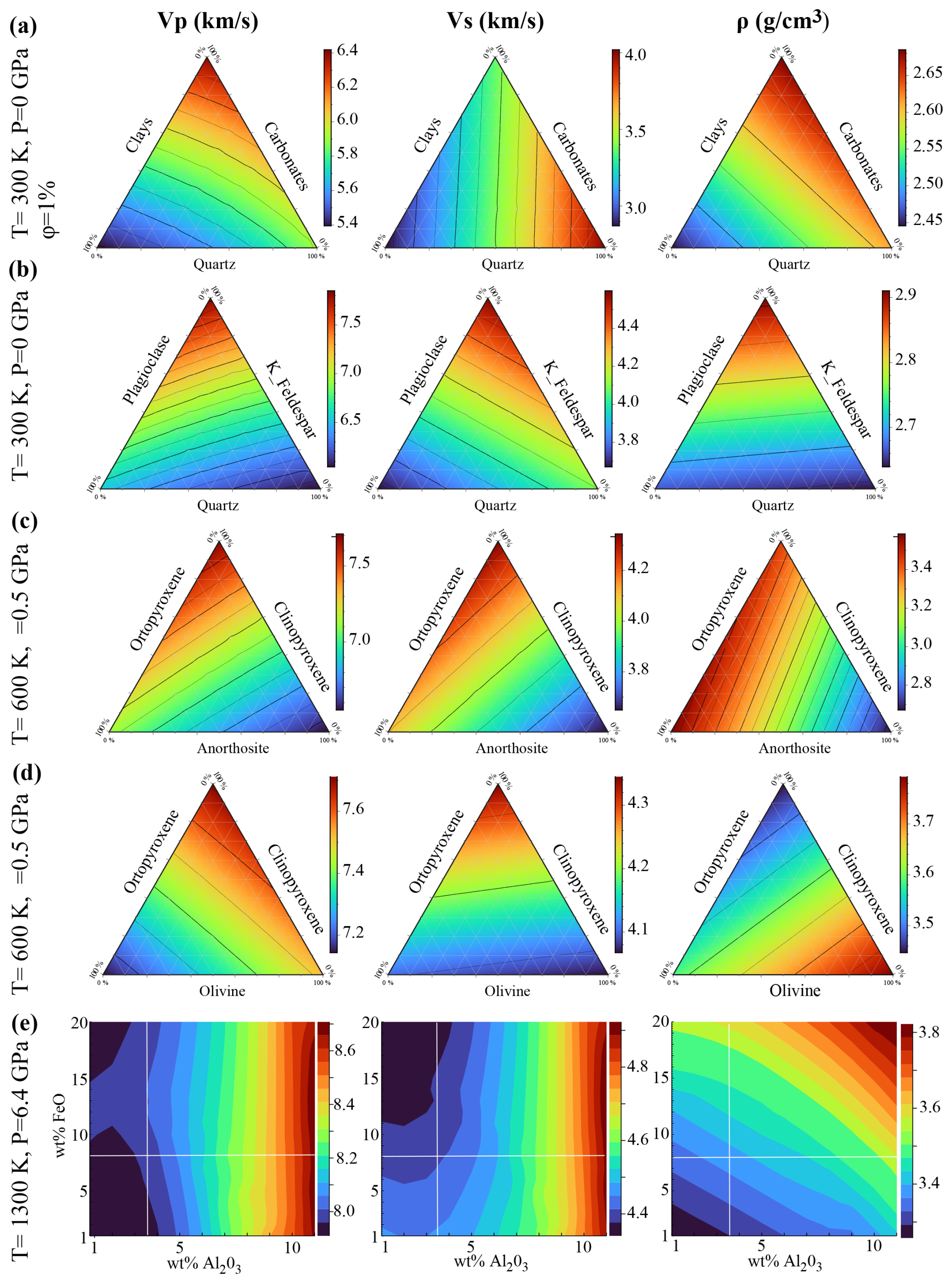
Figure 2 Examples of compressional wavespeed (V_p), shear waves peed (V_s) and density (ρ) variations for: (a) sedimentary, (b) igneous felsic, (c) igneous mafic, (d) igneous ultramafic and (e) mantle rocks as a function of temperature (T), pressure (P), composition and porosity (for sedimentary rocks). All color scales are similar for ease of comparison. In sedimentary rocks (a) carbonates have the higher V_p and ρ. For felsic rocks, with higher percentage of quartz, V_p and ρ becomes higher, while V_s becomes higher with the increase of plagioclase. Also, lower values of all three properties are associated with higher percentage of K-feldspars. For mafic rocks, all properties increase with the percentage of anorthosite and decrease with the percentage of clinopyroxene. Unlike felsic or mafic rocks, in ultramafics, each mineral dominates the decrease of a different property. On (e) the cross marks the average mantle composition.

2.2.4 Mantle Rocks

Compared to the crust, the Earth's mantle petrology is less complex and can be adequately represented by the modal distribution of the main mineral phases (olivine, pyroxenes, and Al-bearing phases) under the consideration of thermodynamic equilibrium (T>500 °C). In this work we determine stable mantle mineral assemblages using a Gibbs free energy minimization scheme (Connolly, 2005, 2009). Therefore, the mantle's physical properties relevant to our work (V_p, V_s and ρ) are computed on these assumptions based on the 𝒯𝒫𝒞 values. A standard characterization of mantle composition is based on the main major oxides in the CFMAS system (CaO–FeO–MgO–Al₂O₃–SiO₂; e.g. Irifune, 1990; Irifune and Tsuchiya, 2015). To simplify the parametrization of 𝒞, here we adopt the discretization of Fullea et al. (2021) where the wt % amounts Al₂O₃ and FeO oxides in the mantle layers are free variables, and CaO–MgO amounts are statistically correlated to Al₂O₃ based on global petrological databases as described in Afonso et al. (2013a). Similarly to Mg# ($=\mathrm{MgO}/[\mathrm{MgO}+\mathrm{FeO}]$), Al₂O₃ has been shown to be a strong compositional indicator and, therefore, an overall proxy for mantle fertility. Mantle fertility refers to the relative enrichment of the mantle in basaltic, melt-producing components, such as basaltic components and thus to its potential to generate partial melting. In particular a fertile mantle should be rich in Al₂O₃, CaO, FeO, meaning more content of clinopyroxene and garnet while a depleted mantle has residue after melt extraction like harzburgitic and low Al₂O₃. In contrast, neither FeO nor SiO₂ are correlated in general with either CaO or Al₂O₃ (Afonso et al., 2013a). For the petrological calculations we use Perple_X (Connolly, 2005, 2009) and for the lower mantle the databases by Xu et al. (2008) and Stixrude and Litgow-Bertelloni (2021). We sample the wide range of 𝒯 (from 100 to 4500 K) and 𝒫 (from 0 to 145 GPa) found in the mantle. As for the self-consistent thermodynamic database, in the upper mantle we use the Xu et al. (2008), whereas in the transition zone and lower mantle we consider Stixrude and Litgow-Bertelloni (2021). 𝒞 values are limited to the ranges of (1–11) wt % for Al₂O₃ and (1–20) wt % for FeO. This range of compositions should be more than enough to model almost every scenario in the entire mantle as values of Al₂O₃ are expected to range from 1.0 to 6.0 wt % and FeO is generally considered to be around 8.0 wt % (e.g., McDonough and Sun, 1995). In some special cases larger ranges might be needed, e.g., Large Low Shear Velocity Provinces in the lowermost mantle (e.g., Vilella et al., 2021). In Fig. 2 we show the relevant mantle properties for several 𝒯𝒫 conditions.

In TCSEIS-1D, there are four major mantle layers defined by their wt % amounts of Al₂O₃ and FeO:

1. The lithospheric mantle extends from the Moho down to the Lithosphere-Asthenosphere Boundary, or LAB (an input depth and temperature are expected from the user as explained in Sect. 2.2). The thickness of this layer is user-defined and does not change unless thermal anomalies are incorporated into the model.

2. The asthenospheric (or sublithospheric) mantle extends from the LAB down to a pressure of ∼14 GPa, representing the average value for the transition from olivine to wadsleyite mineral phases.

3. The transition zone mantle extends from a pressure of ∼14 GPa to a value of ∼24 GPa. The later value is the average pressure for the transition from ringwoodite and majorite to perovskite and ferropericlase, the boundary between the upper and the lower mantle. Note that the transition zone includes an inner phase transition from wadsleyite to ringwoodite at around 520 km depth (Rigden et al., 1991; Tian et al., 2020).

4. The lower mantle extends from a pressure of ∼24 GPa down to the CMB (a user input).

While the boundaries between the first two layers (i.e., LAB depth) and the bottom of the model (i.e., CMB) are input parameters, in the case of the top and bottom of the mantle transition zone, the depth depends on different mineral phase transitions that cannot be predicted beforehand without performing a thermodynamic calculation based on the actual 𝒯𝒫𝒞 conditions. Therefore, our approach here is to initially define those mantle layer boundaries based on standard reference pressure values (∼14 and ∼24 GPa), and subsequently relocate them automatically to the depth at which the relevant phase transitions occur. Therefore, from a compositional point of view, the depth of the base of layer 2 and 3 is effectively defined by a thermodynamic equilibrium calculation. In virtue of the thermodynamic parametrization, the velocity and density jumps related to phase transitions usually associated with the 410, 520, and 660 km discontinuities will arise in the model even if the composition is uniform across all four mantle layers. For example, all these discontinuities still appear in the model for a constant whole mantle composition (e.g., primitive mantle composition with 3.6 wt % Al₂O₃ and 8.0 wt % FeO from McDonough and Sun, 1995). Finally, the user can also specify anomalous regions (compositional anomalies) within any of the four compositional layers by setting a depth range and a chemical anomaly value (e.g., −0.5 wt % Al₂O₃ and +0.2 wt % FeO).

To account for anelasticity, we follow the strategy of Dannberg et al. (2017) and extrapolate the relationships for olivine at upper mantle conditions derived by Jackson and Faul (2010) to the whole mantle. Notice that this is clearly a simplification of the mineralogy at the mantle scale and thus its behavior in seismic attenuation terms, but Dannberg et al. (2017) proved that it yields a useful first-order approximation as the results are not very dissimilar to, for example, the values reported in the PREM model. Here we adopt the parametrization by Dannberg et al. (2017) as described in Appendix B.

Most of the attenuation parameters are different for each major mantle mineral phase. In TCSEIS-1D, we use different attenuation parameters for the most abundant mineral phases at each depth depending on their respective stability fields: the upper mantle (olivine), the upper and lower transition zones (wadsleyite and ringwoodite), and the lower mantle (perovskite). Grain size (d) has a large impact on the attenuation, as per our parametrization described in Appendix B. In the code, the user can choose between three grain size models with depth: (a) a constant value (d=10 mm), (b) the model by Schierjott et al. (2020), in which d increases with depth, and (c) the model by Dannberg et al. (2017), where d decreases with depth. In general terms, we find that the constant and Schierjott models fit best with the general trends of the global 1D models (Fig. 3).

Figure 3 (a) Grain size variation with depth for the 3 models included in the code: Constant (a constant value of 10⁻² m), Schierjott (the grain size variations estimated by Schierjott et al., 2020) and Dannberg (the grain size variations estimated by Dannberg et al., 2017). (b) Several 1D radial models of Q_s for the whole mantle: SL8 (Anderson and Hart, 1978), QM1 (Widmer et al., 1991), QL6 (Durek and Ekstrom, 1996), QLM9 (Lawrence and Wysession, 2006), QOS08 (Oki and Shearer, 2008), PREM (Dziewonski and Anderson, 1981). (c) Q_s computed from the Burguers model of linear viscoelasticity (Jackson and Faul, 2010). The Constant and Schierjott models produce the closest fit to the radial models.

2.2.5 Melt

Accounting for melt in a 1D column requires the definition of consistent solidus and liquidus curves for the crust and the whole mantle. In the crust, we consider the equations in Gerya (2019) characterizing the solidus and liquidus temperatures for sediments and igneous rocks. In the mantle, water content and, to a lesser extent, composition control the solidus values reported in the literature (e.g., Schmidt and Poli, 1998; Hirschmann, 2000; Katz et al., 2003; Sarafian et al., 2016; Fu et al., 2018). In TCSEIS-1D, we allow the user to define the solidus curve for the upper mantle (i.e., from the Moho to a pressure of ∼10 GPa or depth of ∼300 km) from two sources:

• The solidus presented by Andrault et al. (2018), which corresponds to a nominally dry mantle (between 1 and 90 wt ppm),

• The second-degree polynomial by Katz et al. (2003), defined only up to 7 GPa, which corresponds to a nominally anhydrous mantle with 40–80 wt ppm of water.

From 10 to 30 GPa, we use the logarithmic anhydrous solidus curve by Herzberg et al. (2000), and from 30 to 120 GPa, the solidus curve by Fu et al. (2018) with ∼400 wt ppm water can be extrapolated to the CMB conditions, according to the authors.

For the mantle liquidus, we use (a) a fourth-degree polynomial fitted to the liquidus curve by Litasov and Ohtani (2002), valid from 0 GPa (surface) to ∼30 GPa (roughly 800 km depth), and (b) a second-degree polynomial fitting the liquidus curve by Fu et al. (2018) from 30 GPa to the CMB. With this parametrization, the solidus and liquidus curves have large jumps at the crust-mantle boundary and around 800 km, therefore we have chosen to smooth them with a rloess (Fig. 4).

The volumetric melt fraction (Melt) is usually defined, for a constant pressure, as a linearly varying temperature-dependent function (e.g., Gerya and Yuen, 2003b; Burg and Gerya, 2005; Gerya, 2019; Fullea et al., 2021):

$$\begin{array}{}\text{(4)}& {\displaystyle }\mathrm{\text{Melt}}=\mathrm{0}\mathit{\%}\text{ from }T\le T_{\text{solidus}}\text{(5)}& {\displaystyle }\begin{array}{rl}\text{Melt}={\displaystyle \frac{(T-T_{\text{solidus}})}{(T_{\text{liquidus}}-T_{\text{solidus}})}}& \mathrm{100}\\ & \text{from }{T}_{\text{solidus}}<T<T_{\text{liquidus}}\end{array}\text{(6)}& {\displaystyle }\text{Melt}=\mathrm{100}\mathit{\%}\text{ at }T\ge T_{\text{liquidus}}\end{array}$$

where T_solidus and T_liquidus are the wet solidus and dry liquidus temperatures defined by the curves described previously. Once Melt(z) has been computed for each model node, the associated seismic parameters (V_p, V_s, Q_s) are corrected following the experimental study by Chantel et al. (2016):

$$\begin{array}{}\text{(7)}& {\displaystyle }{V}_{\mathrm{P}}=\mathrm{0.07}{\text{Melt}}^{\mathrm{2}}-\mathrm{0.5566}\text{Melt}+\mathrm{7.9235}\text{(8)}& {\displaystyle }{V}_{\mathrm{S}}=\mathrm{0.065}{\text{Melt}}^{\mathrm{2}}-\mathrm{0.5565}\text{Melt}+\mathrm{4.4211}\text{(9)}& {\displaystyle }\mathrm{100}/Q_{\mathrm{S}}=\mathrm{2.4063}\ln \left(\text{Melt}\right)+\mathrm{5.9284}\end{array}$$

Mantle density is corrected (becoming the effective density, ρ_eff) by the equation postulated by Gerya (2019):

$$\begin{array}{}\text{(10)}& {\mathit{\rho }}_{\text{eff}}={\mathit{\rho }}_{\text{solid}}\left(\mathrm{1}-\text{Melt}+\text{Melt}{\displaystyle \frac{{\mathit{\rho }}_{\text{0molten}}}{{\mathit{\rho }}_{\text{0solid}}}}\right)\end{array}$$

where ρ_0solid and ρ_0liquid are the standard densities of the solid and molten rock, respectively, and ρ_solid is the density of the solid rock at the given 𝒯𝒫 conditions computed as described in Sects. 2.1 and 2.3. The values for ρ_0solid and ρ_0liquid are taken from the compilation of values by Gerya (2019) and could be changed by the user inside the code if required. Figure 4 shows the used curves.

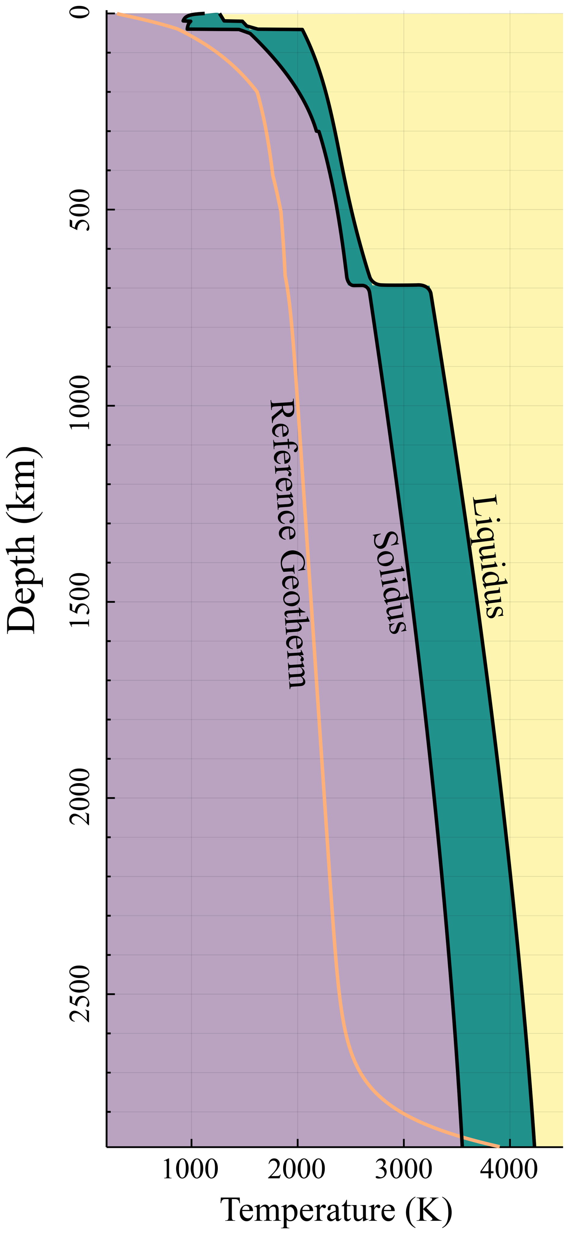
Figure 4 Solidus and liquidus curves from the entire crust and mantle. Solidus by: Gerya (2019), Katz et al. (2003), Herzberg et al. (2000) and Fu et al. (2018). Liquidus by: Gerya (2019), Litasov and Ohtani (2002) and Fu et al. (2018). See text for details.

2.3 Surface Wave Dispersion Forward Modeling

TCSEIS-1D computes surface wave dispersion curves in two ways: from a native function SWD.jl (developed as part of TCSEIS-1D) or by calling Mineos.jl, a Julia wrapper around the code Mineos developed to compute normal modes of the Earth (Master et al., 2011, https://geodynamics.org/cig, last access: 17 February 2026). In general terms, SWD.jl is faster than Mineos.jl, although the former gives an approximated solution in contrast to the exact solution from the latter. Both codes run on CPU and the computation time for a dispersion curve with 20 samples, for PREM model is in the order of 0.17 s for SWD.jl and 0.26 s for Mineos.jl on an Apple MacBook Air with 8 GB of RAM and M1 chip. Also, the approximations built in SWD.jl yield some high errors (>1 %) in cases of very strong attenuation (Q_s<70) and high-order overtone calculation.

SWD.jl is mostly based on the formulation described by Haney and Tsai (2015, 2017, 2019). These authors utilize (for both Rayleigh and Love waves) a finite element approach based on the thin-layer method (Lysmer, 1970; Kausel, 2005). The scheme behind SWD.jl and the corrections necessary to approximate the results from Mineos.jl are detailed in Appendix A. To validate both approaches, in Fig. 5, we present a comparison between surface wave dispersion curves computed by SWD.jl (the main TCSEIS-1D dispersion engine), Mineos.jl (Masters et al., 2011) and the exact solution. Each code uses a different approach for the computation: SWD.jl uses a finite element solution, whereas Mineos uses the traditional normal-mode summation. Discrepancies in the results from all three codes are small in terms of phase velocity (dc<0.045 %) and group velocity (dU<0.2 %) and might arise from the difference in the computations and/or parameterization of the model for each code. For example, at T=50 s, considering the PREM velocity model as input, the fundamental mode Rayleigh wave phase velocity differences comparing the output of the three codes are <0.002 %. Notice that errors increase with time because of the spherical approximation. The user can always extract the standard seismic velocities and density geophysical model from the TCSEIS-1D output to perform customized seismic modeling a posteriori with other tools. We recommend using Mineos.jl for modeling data with long periods (T>70 s, shorter periods are properly represented by SWD.jl), higher overtones (overtones 1 and 2 are well computed by SWD.jl but higher overtones are not well represented by the FEM formulation), and for studying regions with strong attenuation (as SWD.jl uses an approximation to attenuation, see Appendix B for details). Note that the original Mineos code has a limitation of 300 velocity layers, making it only appropriate for T>30 s. On the other hand, SWD.jl is recommended for shorter periods (T<70 s; mainly crust and upper mantle studies) where complex models can be proposed or when computational time is relevant.

Figure 5 Comparison between surface wave dispersion curves computed by SWD.jl (red, the main TCSEIS-1D dispersion engine), Mineos (green, Masters et al., 2011) and the exact solution (blue circles marked as Nolet).

2.4 Receiver Functions Forward Modeling

In order to give the user a basic handling of receiver function data during the modeling stages, we have incorporated a simple module (i.e., the computation is made without accounting for the effect of anisotropy or attenuation) to compute synthetic receiver functions from the input geophysical model. Receiver functions are computed using a transfer function between the stress and displacement known as the propagator matrix approach (Thomson, 1950; Haskell, 1953; Kennett, 1983). For all the receiver functions, P-to-S, S-to-P, and SKS-to-P, the sequence is similar. For each source (with a depth and epicentral distance taken from the IASP91 tables; Kennett et al., 1991), the synthetic radial and vertical components (R and Z) are computed for a given 1D model and then rotated into the direction of polarization of the incident P-wave (L) and its perpendicular (Q) in the R-Z plane (e.g., Vinnik, 1977; Kind et al., 1995). In general, we compute the surface response in the Fourier domain for a plane impingement waveform. The transmitted impulse is assumed to arrive at the surface at t=0 s. Then, we calculate the time domain displacements at the surface for each direction. The computation includes all multiples, transformations, and reflections produced by an arbitrary structure with homogeneous layers (Svenningsen and Jacobsen, 2007). Finally, the Z (or L) component records are deconvolved from the R (or Q) components, and a Gaussian low-pass filter is applied to the resulting seismogram. For the S wave incidence, the resultant seismograms are subject to time and sign reversals, following the convention for S receiver functions (e.g., Yuan et al., 2006). This process is repeated n times (as many RFs are input by the user) for a list of events (epicentral distances and depths). The resulting n receiver functions are stacked via move-out correction considering the IASP91 model and a reference velocity of 6.4 km s⁻¹ (e.g., Rondenay, 2009). The final stacked receiver functions are compared with the observed waveforms to measure misfits. Figure 6 shows a comparison between the results of the RF computations in TCSEIS-1D and those from other codes in order to validate the results.

For these comparisons (and by default in the code), RF are normalized, as amplitude values may vary with instruments and processing. No other corrections are applied to the final stack, and the post-processing (if required) is left to the end user. Furthermore, attenuation and anisotropy effects are not accounted for, the code automatically outputs a geophysical model (z, V_p, V_s, ρ, Q_s, χ) that can be used for forward computation and individual RF for post-processing using other modelling tools. It is important to keep in mind that real RF are highly dependent on the quality of the data and the steps used by the interpreter. In general, there are several ways to approach the deconvolution of the horizontal and vertical components of the seismogram that may differ from the scheme presented here (e.g., Pesce, 2010). Here, we use the now-classic implementation of the frequency-domain water-level algorithm (e.g., Langston, 1979; Rondenay, 2009). Hence, when modeling real RF with TCSEIS-1D, care must be taken to consider the aforementioned points for consistency, especially regarding anisotropy and attenuation.

Figure 6 Comparison between the synthetic Receiver Functions (RF) computed by the code and those computed with other codes. (a) P-to-S RF, (b) S-to-P RF and (c) SKS-to-P RF. RF in red correspond to our code, those in black were computed with the Matlab codes by Bo Holm Jacobsen (2008; Svenningsen and Jacobsen, 2007), and in green those computed in IRFFM2 V1.2 (Tkalčić et al., 2015, only P-to-S available). Differences are small (error <0.1 %). For this example, the Gaussian parameter a=2.5 (roughly between 0.4 and 1 Hz).

3 Testing TCSEIS-1D: Sensitivity analysis

To illustrate the capabilities of TCSEIS-1D, we present three simple examples that demonstrate the sensitivity of Rayleigh wave phase velocity curves and P-to-S receiver functions to compositional and temperature variations with respect to a reference model (Figs. 7–10). The reference model in our examples is characterized by:

• i.

  A 40 km-thick crust with a 2 km shale sedimentary layer (Qz(%)=30, Carbo(%)=10, Clays(%)=60, Porosity(%)=5), a 20 km thick monzodioritic (felsic) upper crust (Qz(%)=10, K-feldspar(%)=90, Plagioclase(%)=0), and a 20 km thick orthopyroxene-gabbroic (mafic) lower crust (Anorthosite(%)=20, Clinopyroxene(%)=60, Orthopyroxene(%)=20).

• ii.

  A 200 km-thick lithosphere with a LAB temperature of 1300 °C.

• iii.

  A uniform whole mantle composition: Al₂O₃=3.6 wt % and FeO=8.0 wt % (e.g., McDonough and Sun, 1995) with constant grain size (10 mm).

• iv.

  Isotropic model (i.e., no radial anisotropy)

3.1 Example 1: Average Mantle Composition

In this first example (Fig. 7), we change the composition of the entire mantle. The values for the two independent oxides in our parametrization (Al₂O₃=3.6 wt % and FeO=8.0 wt %) correspond to the primitive mantle composition from McDonough and Sun (1995). Here, we explore the effect of changing the value of Al₂O₃ to 2.0 wt % and to 5.0 wt % (for a constant value of FeO wt %). Then, the effect of changing the values of FeO to 6.0 % and 10.0 % (for a constant value of Al₂O₃ wt %). From this simple test, we can draw a few important conclusions:

• The amount of Al₂O₃ dominates the velocity gradients in the upper mantle, with velocity variations being proportional to Al₂O₃ content. However, Al₂O₃ has a limited effect on the lower mantle.

• The amount of FeO dictates the velocity gradients in the lower mantle while having a minor effect in the upper mantle. In general terms, velocity gradients are inversely proportional to the wt % of FeO in the lower mantle. Interestingly FeO has a dramatic effect on the gradient at the top of the D” layer, changing its depth by ∼100 km within our test.

• The sharpness and depth of the transition zone boundaries is controlled by mantle composition. Both Al₂O₃ and FeO appear to have a dramatic effect on the 410 km discontinuity (olivine→wadsleyite) sharpness. By contrast, the 560 km discontinuity (wadsleyite→ringwoodite) and the 660 km discontinuity (ringwoodite + majorite → perovskite + ferropericlase) are mostly affected by FeO and Al₂O₃ respectively.

We note that within the chemical parametrization in TCSEIS-1D, the amount of CaO and MgO oxides is dependent on the amount of Al₂O₃ based on statistical correlations from global petrological databases (Afonso et al., 2013a). By contrast, the amount of FeO is an independent variable.

Figure 7 Example 1. Comparison between the results of a constant composition mantle in TCSEIS-1D (solid lines) and the PREM model (dashed). Here we have tested several compositions to show how large V_p, V_s and ρ anomalies can arise from extreme values of Al₂O₃ and FeO. Top panels show the comparison in absolute V_p, V_s and ρ values, while the bottom panel shows anomalies with respect to PREM. In the bottom panel, crustal anomalies have been deleted from the presentation as they are too large since PREM has a poorly estimated crust.

3.2 Example 2: Cold horizontally stagnating slab

In the second example (Fig. 8), we implement a thermal and compositional anomaly with respect to the reference model representing a 1D section of a cold horizontally stagnating slab (a subducted slab that changes direction in the transition mantle; e.g., Fukao et al., 2009). The anomaly is defined from 300 to 500 km depth (Fig. 14) and is characterized by: (a) a −600 K thermal anomaly with respect to the ambient mantle; and (b) a chemical anomaly of ${\mathrm{Al}}_{\mathrm{2}}{\mathrm{O}}_{\mathrm{3}}=-\mathrm{0.25}$ wt % with respect to our reference model. The mantle in the “slab” region shows higher values for velocities, density, and Q_s than the reference model. These positive anomalies are easily recognized in the Rayleigh wave dispersion curves: for the long periods in the fundamental mode and, in general, for the higher dispersion modes, the phase velocity anomalies are $>+\mathrm{3}$ %. The P-to-S receiver function is only modified for periods >20 s (arrival of late phases) due to the upward shift of the 410 km discontinuity caused by the “slab” anomaly.

Figure 8 Example 2 showing the effect of a cold slab-like feature plunging into the transition zone. On the top: the left panel show the V_p, V_s and ρ profiles with depth (solid lines are the computed parameters and dashed ones are the PREM values), in the center we shows the temperature profile with (T) and without (Ref T), and on the right the attenuation profile with (Q_s) and without the slab (Q_s Ref). On the center of the figure we present: on the left the dispersion curves of the model with (solid lines) and without (circles) the slab for the fundamental mode (blue) and the 1st (orange) and second (green) overtones. Anomalies between both are presented in the right panel. At the bottom P-to-S RF with (black) and without (blue) are shown. Notice that, except for the first panel, Ref is the reference model without anomalies (see text for details).

3.3 Example 3: Hot ponding plume head

In the third example (Fig. 9), we implement a thermal and compositional anomaly with respect to the reference model representing a 1D section of a hot horizontally flowing or ponding plume head (wide horizontal zones that extend from the vertical plume-conduct at discontinuities; e.g., Dongmo Wamba et al., 2023). The “plume” is the anomaly, which is defined from 600 to 900 km depth (Fig. 15) and is characterized by: (a) a +600 K thermal anomaly with respect to the ambient mantle; and (b) a chemical anomaly of ${\mathrm{Al}}_{\mathrm{2}}{\mathrm{O}}_{\mathrm{3}}=+\mathrm{0.25}$ wt % and $\mathrm{FeO}=+\mathrm{0.5}$ wt %. The “plume” anomaly shows lower values for the velocities, density, and Q_s than the reference model. In this case, the anomalous region is divided into two sections: the upper part (600–700 km depth) with extremely low anomalies (caused by melting atop the plume), and the lower part (depth >700 km) where the decrease in the physical parameters is less pronounced. The temperature and composition anomalies strongly affect synthetic Rayleigh wave dispersion curves. For the long periods in the fundamental mode, and in general for the higher dispersion modes, the phase velocity anomalies are $<-\mathrm{5}$ %. The P-to-S receiver function is modified for periods >40 s as all the lower part of the transition zone is affected by the anomaly, which also generates sharp impedance contrasts. It is worth noting that the effect of the anomaly in this example is so significant that the crustal phases recorded in the receiver functions are slightly affected as well.

Figure 9 Example 3 showing the effect of a hot plume-like feature entering the transition zone from below. Panels are in the same configuration as in Fig. 8, but in this case we add the melt curve to the top right plot.

3.4 Example 4: Thin Lithosphere

In the final example, we leave most parameters from the reference model constant and change the base of the lithosphere from 200 km in the reference model to 60 km (Fig. 16). This change has a drastic effect on the model as two melt regions appear, one near the LAB and the other at the base of the crust, causing two low-velocity, density, and Q_s regions at 35 and 70 km depth, respectively. The effect of the lithospheric thinning is strong in the predicted surface wave dispersion curves, in particular for the fundamental mode, where large negative anomalies are apparent, and less so for the overtones. The waveform of the P-to-S receiver function drastically changes due to the negative-impedance present within the crust and upper mantle in our example model. The effect is much less dramatic but still present if the melt modeling option is turned off.

Figure 10 Example 4 showing the effect of a thin lithosphere under an average continental crust. Panels are the same as in Fig. 8. Here we show two outputs: with melt (MELT, same as in previous examples) and without melt (NO MELT, dotted lines).

4 Remarks, conclusions and further work

Receiver functions and surface wave dispersion data analysis has led to remarkable results revealing the Earth's internal structure in terms of compressional and shear waves velocity anomalies (δV_p, δV_s). Yet, the interpretation of these anomalies in terms of crustal and mantle composition is a challenging modeling task. The usage of these data under geophysical-petrological schemes has proven to yield important results in terms of the thermal and petrological structure of the Earth's mantle (e.g. Munch et al., 2018, 2021; Bissig et al., 2021; Afonso et al., 2022; Fullea et al., 2021; Lebedev et al., 2024). Yet, the usage of this type of method is not common.

In order to build a bridge to go from classical seismological approaches to the thermal-petrological realm, we present TCSEIS-1D, a new, open-source, cross-platform, easy-to-use, and accurate code to model the crust and whole mantle using surface wave dispersion curves (including group and phase velocity of Rayleigh and Love waves for the fundamental mode, as well as several overtones) and three widely used receiver functions (P-to-S, S-to-P, and SKS-to-P) directly in terms of rock composition and the in-situ temperature and pressure conditions. We achieved this by creating an interface between the modeling of seismic data and mineral/phase equilibria calculations that allow for the calculation of elastic properties (i.e., V_p, V_s, and density) as a function of temperature, pressure, and composition. Moreover, TCSEIS-1D can be used as a simple geophysical model (i.e., seismic velocities and density) generator based on input thermochemical conditions that can be coupled to third-party seismic codes to perform forward calculations, offering as well a variety of tools intended to interpret geophysical data and models in petrological (e.g., property maps in the 𝒯𝒫𝒞 space; Fig. 1) and geodynamical terms (e.g. different thermal scenarios, Figs. 14–16).

TCSEIS-1D can be used to simultaneously fit different real seismological and other geophysical data sets within a trial-and-error approach or to carry out synthetic modeling (e.g., sensitivity analysis), making it a useful tool for a wide range of geoscientists. Future work includes developing an inversion scheme of seismic data for the thermochemical structure of the crust and mantle based on TCSEIS-1D.

Appendix A: TCSEIS-1D Surface Wave Dispersion native package: SWD.jl

SWD.jl is mostly based on the formulation described by Haney and Tsai (2015, 2017, 2019). These authors utilize (for both Rayleigh and Love waves) a finite element approach based on the thin-layer method (Lysmer, 1970; Kausel, 2005). In contrast to the popular Thomson-Haskell recursion formula (e.g., Takeuchi and Saito, 1972; Saito, 1988), Haney and Tsai employed several thin layers leading to a generalized eigenvalue/eigenvector problem that must be solved for every sampled frequency ($\mathrm{1}/T_{\text{Observed}}$, Hz). Their method is both accurate and fast and allows for the consideration of a water layer on top of the model column. However, as originally proposed, the method is hampered by two shortcomings: (1) it assumes the Earth is isotropic, elastic and flat, and (2) it requires the specification of a relatively dense Finite Elements (FEM) mesh. We address each one of these as follows:

• (a)

  We decouple the computation of Rayleigh and Love waves based on the vertically and horizontally polarized V_s(𝒯𝒫𝒞) components, V_SV and V_SH, respectively defined as:

  $$\begin{array}{}\text{(A1)}& {\displaystyle }{V}_{\text{SV}}=\left(\mathrm{1}-{\displaystyle \frac{\mathrm{1}}{\mathrm{3}}}\mathit{\chi }\right)V_{\mathrm{S}}\text{(A2)}& {\displaystyle }{V}_{\text{SH}}=\left({\displaystyle \frac{\mathrm{2}}{\mathrm{3}}}\mathit{\chi }+\mathrm{1}\right)V_{\mathrm{S}}\end{array}$$

  Where χ is the average seismic radial anisotropy for each layer (user input). Rayleigh and Love dispersion curves are computed as a function of V_SV and V_SH respectively.

We include anelastic effects as stated by Karato (1993), Minster and Anderson (1981), Afonso et al. (2005), Fullea et al. (2021), using the expressions:

$$\begin{array}{}\text{(A3)}& {\displaystyle }{V}_{\text{Pa}}=V_{\mathrm{P}}\left(\mathrm{1}-{\displaystyle \frac{\mathrm{2}}{\mathrm{9}}}\cot \left({\displaystyle \frac{\mathit{\pi }\mathit{\alpha }}{\mathrm{2}}}\right)Q_{\mathrm{s}}^{-\mathrm{1}}\right)\text{(A4)}& {\displaystyle }{V}_{\text{Sa}}=V_{\mathrm{s}}\left(\mathrm{1}-{\displaystyle \frac{\mathrm{1}}{\mathrm{2}}}\cot \left({\displaystyle \frac{\mathit{\pi }\mathit{\alpha }}{\mathrm{2}}}\right)Q_{\mathrm{s}}^{-\mathrm{1}}\right)\end{array}$$

Where, V_Pa and V_Sa are the anelastic P and S velocities, and V_p and V_s are the anharmonic velocities computed from 𝒯𝒫𝒞 values. Further details on estimating Q_s are presented in Sect. 2.6.

• (b)

  We consider the Earth's sphericity correcting the values of V_p, V_s and ρ for the Earth-flattening approximation before computing the dispersion curves. Here, we follow Herrmann (2013) for Rayleigh waves, and the equations by Schwab and Knopoff (1972) for Love waves. The depth from the surface in the equivalent flat Earth model, z, is given by:

  $$\begin{array}{}\text{(A5)}& z=a\ln {\displaystyle \frac{a}{r}}\end{array}$$

  Where r is the radial distance from the center of the Earth, and a is the Earth's radius. Hence, if we consider a spherical layer bounded by r_i and r_i−1 radii, with $r_{i-\mathrm{1}}>r_i$, then the thickness, h, of the corresponding ith flat layer is given by:

  $$\begin{array}{}\text{(A6)}& (h_i{)}_{\mathrm{f}}=a\ln \left({\displaystyle \frac{a}{r_i}}\right)-a\ln \left({\displaystyle \frac{a}{r_{i-\mathrm{1}}}}\right)\end{array}$$

The mean V_p, V_s and ρ in the transformed flat layer model, $(V_{{\mathrm{p}}_i}{)}_{\mathrm{f}}$, $(V_{{\mathrm{s}}_i}{)}_{\mathrm{f}}$, (ρ_i)_f and are given by

$$\begin{array}{}\text{(A7)}& {\displaystyle }(V_{{\mathrm{p}}_i}{)}_{\mathrm{f}}=(V_{{\mathrm{p}}_i}{)}_{\mathrm{s}}{\displaystyle \frac{\mathrm{2}a}{r_i+r_{i-\mathrm{1}}}}\text{(A8)}& {\displaystyle }(V_{{\mathrm{s}}_i}{)}_{\mathrm{f}}=(V_{{\mathrm{s}}_i}{)}_{\mathrm{s}}{\displaystyle \frac{\mathrm{2}a}{r_i+r_{i-\mathrm{1}}}}\text{(A9)}& {\displaystyle }({\mathit{\rho }}_i{)}_{\mathrm{f}}=({\mathit{\rho }}_i{)}_{\mathrm{s}}{\left({\displaystyle \frac{\mathrm{2}a}{r_i+r_{i-\mathrm{1}}}}\right)}^{\text{SE}}\end{array}$$

Where $(V_{{\mathrm{p}}_i}{)}_{\mathrm{s}}$, $(V_{{\mathrm{s}}_i}{)}_{\mathrm{s}}$, (ρ_i)_s are the mean V_p, V_s and ρ in the spherical model, and SE is a parameter that takes a different value for Love ($\text{SE}=-\mathrm{5}$, Schwab and Knopoff, 1972) and Rayleigh (we find a better fit with an exponent value of $\text{SE}=-\mathrm{2.278}$ instead of $\text{SE}=-\mathrm{2.275}$ as originally reported in Herrmann, 2013).

• (c)

  Finally, we optimize the FEM mesh for the forward computation (e.g., Xia et al., 1999; Ma and Clayton, 2016; Hanney and Tsai, 2015, 2017, 2019). Generally, the required mesh must have adequate sampling above the sensitivity depth of each period, without oversampling the model below it unnecessarily. As a rule of thumb, more than five 5 layers (6 nodes) are required in the sensitivity depths of each frequency with their thicknesses increasing exponentially from the surface to the bottom of the model (e.g., Hanney and Tsai, 2017). In TCSEIS-1D, the user has two possibilities: (i) using a precomputed mesh (the Golden Mesh) created with smaller layers than those required to compute the dispersion at any period between 1 and 500 s, and slightly oversampling the base of the model; or (ii) using a new mesh based on the lowest period of the input data and a low threshold of Rayleigh wave phase velocity set to 1 km s⁻¹ (see Hanney and Tsai, 2017, Appendix D for more details). Our mesh samples all the space, and the thickness of each layer coincides with the sensitivity of both Rayleigh waves and Love waves (depending on the period). Our FEM grids for surface waves are designed to compute dispersion curves in the period range from 5 to 500 s.

Appendix B: Seismic attenuation model

Dannberg et al. (2017) pose that the response of a continuum that behaves according to Burgers model of linear viscoelasticity with creep function in response to a sinusoidally time-varying stress (e.g., a dispersive wave) is given by the dynamic compliance J^∗(ω) (the Laplace transform of its creep function). This function takes the form:

$$\begin{array}{}\text{(B1)}& {\displaystyle }{J}^{\ast }\left(\mathit{\omega }\right)=J_{\mathrm{1}}\left(\mathit{\omega }\right)+\mathrm{i}{J}_{\mathrm{2}}\left(\mathit{\omega }\right)\text{(B2)}& {\displaystyle }\begin{array}{rl}{J}_{\mathrm{1}}& =J_u\mathit{\{}\mathrm{1}+{\displaystyle \frac{\mathit{\alpha }{\mathrm{\Delta }}_{\mathrm{B}}}{{\mathit{\tau }}_H^{\mathit{\alpha }}-{\mathit{\tau }}_L^{\mathit{\alpha }}}}{\int }_{{\mathit{\tau }}_L}^{{\mathit{\tau }}_H}{\displaystyle \frac{{\mathit{\tau }}^{\mathit{\alpha }-\mathrm{1}}}{\mathrm{1}+{\mathit{\omega }}^{\mathrm{2}}}}\mathrm{d}\mathit{\tau }\\ & +{\displaystyle \frac{{\mathrm{\Delta }}_{\mathrm{P}}}{\mathit{\sigma }\sqrt{\mathrm{2}\mathit{\pi }}}}{\int }_{\mathrm{0}}^{\mathrm{\infty }}{\displaystyle \frac{\mathrm{1}}{\mathit{\tau }(\mathrm{1}+{\mathit{\omega }}^{\mathrm{2}}{\mathit{\tau }}^{\mathrm{2}})}}\exp (-{\displaystyle \frac{\ln (\frac{\mathit{\tau }}{{\mathit{\tau }}_{\mathrm{P}}}{)}^{\mathrm{2}}}{\mathrm{2}{\mathit{\sigma }}^{\mathrm{2}}}})\mathrm{d}\mathit{\tau }\mathit{\}}\end{array}\text{(B3)}& {\displaystyle }\begin{array}{rl}{J}_{\mathrm{2}}=J_u\mathit{\{}& {\displaystyle \frac{\mathit{\omega }\mathit{\alpha }{\mathrm{\Delta }}_{\mathrm{B}}}{{\mathit{\tau }}_H^{\mathit{\alpha }}-{\mathit{\tau }}_L^{\mathit{\alpha }}}}{\int }_{{\mathit{\tau }}_L}^{{\mathit{\tau }}_H}{\displaystyle \frac{{\mathit{\tau }}^{\mathit{\alpha }}}{\mathrm{1}+{\mathit{\omega }}^{\mathrm{2}}{\mathit{\tau }}^{\mathrm{2}}}}\mathrm{d}\mathit{\tau }\\ & +{\displaystyle \frac{\mathit{\omega }{\mathrm{\Delta }}_{\mathrm{P}}}{\mathit{\sigma }\sqrt{\mathrm{2}\mathit{\pi }}}}{\int }_{\mathrm{0}}^{\mathrm{\infty }}{\displaystyle \frac{\mathrm{1}}{\mathrm{1}+{\mathit{\omega }}^{\mathrm{2}}{\mathit{\tau }}^{\mathrm{2}}}}\exp (-{\displaystyle \frac{\ln (\frac{\mathit{\tau }}{{\mathit{\tau }}_{\mathrm{P}}}{)}^{\mathrm{2}}}{\mathrm{2}{\mathit{\sigma }}^{\mathrm{2}}}})\mathrm{d}\mathit{\tau }\\ & +{\displaystyle \frac{\mathrm{1}}{\mathit{\omega }{\mathit{\tau }}_M}}\mathit{\}}\end{array}\end{array}$$

Where ω is the angular frequency, $\mathit{\omega }=\mathrm{2}\mathit{\pi }/T$, α is the anelastic frequency exponent, Δ_B is the Burgers element strength and Δ_P and σ are the peak height and width, and J_u is the unrelaxed compliance (which is not computed for Q_s estimations).

All the timescales τ_i control the temperature, pressure, and grain size sensitivity of the anelastic scaling relationships:

$$\begin{array}{}\text{(B4)}& \begin{array}{rl}{\mathit{\tau }}_i& ={\mathit{\tau }}_{\text{iR}}{\left({\displaystyle \frac{d}{d_{\mathrm{R}}}}\right)}^{\text{mi}}\\ & \times \exp \left[\left({\displaystyle \frac{E^{\ast }}{R}}\right)\left({\displaystyle \frac{\mathrm{1}}{T}}-{\displaystyle \frac{\mathrm{1}}{T_{\mathrm{R}}}}\right)+\left({\displaystyle \frac{V^{\ast }}{R}}\right)\left({\displaystyle \frac{P}{T}}-{\displaystyle \frac{P_{\mathrm{R}}}{T_{\mathrm{R}}}}\right)\right]\end{array}\end{array}$$

where $i=H,L,P,M$ are the upper, lower, peak and Maxwell viscous relaxation values respectively, and all m_j are grain size exponents with $j=H,L,P$ for anelastic relaxation (m_a), and j=M for viscous relaxation (m_v). Here, E^∗ and V^∗ are the activation energy and volume for the anelastic model. We use the same values for each major mantle zone as reported in the supplementary material of Dannberg et al. (2017). The temperature, pressure, and grain size sensitivity of the anelastic relationships are introduced in terms of reference values T_R, P_R and d_R.

$$\begin{array}{}\text{(B5)}& Q_{\mathrm{s}}={\displaystyle \frac{J_{\mathrm{1}}\left(\mathit{\omega }\right)}{J_{\mathrm{2}}\left(\mathit{\omega }\right)}}\end{array}$$

and

$$\begin{array}{}\text{(B6)}& Q_{\mathrm{p}}={\displaystyle \frac{\mathrm{9}}{\mathrm{4}}}{Q}_{\mathrm{s}}\end{array}$$

which implies an infinite quality factor for the bulk modulus (e.g., Karato, 1993; Minster and Anderson, 1981).