the Creative Commons Attribution 4.0 License.
the Creative Commons Attribution 4.0 License.
 | 23 Oct 2019
Pore-scale permeability prediction for Newtonian and non-Newtonian fluids
Philipp Eichheimer
Marcel Thielmann
Anton Popov
Gregor J. Golabek
Wakana Fujita
Maximilian O. Kottwitz
Boris J. P. Kaus
The flow of fluids through porous media such as groundwater flow or magma migration is a key process in geological sciences. Flow is controlled by the permeability of the rock; thus, an accurate determination and prediction of its value is of crucial importance. For this reason, permeability has been measured across different scales. As laboratory measurements exhibit a range of limitations, the numerical prediction of permeability at conditions where laboratory experiments struggle has become an important method to complement laboratory approaches. At high resolutions, this prediction becomes computationally very expensive, which makes it crucial to develop methods that maximize accuracy. In recent years, the flow of non-Newtonian fluids through porous media has gained additional importance due to, e.g., the use of nanofluids for enhanced oil recovery. Numerical methods to predict fluid flow in these cases are therefore required.
Here, we employ the open-source finite difference solver LaMEM (Lithosphere and Mantle Evolution Model) to numerically predict the permeability of porous media at low Reynolds numbers for both Newtonian and non-Newtonian fluids. We employ a stencil rescaling method to better describe the solid–fluid interface. The accuracy of the code is verified by comparing numerical solutions to analytical ones for a set of simplified model setups. Results show that stencil rescaling significantly increases the accuracy at no additional computational cost. Finally, we use our modeling framework to predict the permeability of a Fontainebleau sandstone and demonstrate numerical convergence. Results show very good agreement with experimental estimates as well as with previous studies. We also demonstrate the ability of the code to simulate the flow of power-law fluids through porous media. As in the Newtonian case, results show good agreement with analytical solutions.
- Article
(4925 KB) - Full-text XML
- BibTeX
- EndNote


Fluid flow within rocks is of interest for several Earth science disciplines including petrology, hydrogeology and petroleum geoscience, as fluid flow is relevant to the understanding of magma flow, groundwater flow and oil flow, respectively (Manwart et al., 2002). Permeability estimates can be inferred on several scales ranging from macroscale (crust) (Fehn and Cathles, 1979; Norton and Taylor Jr., 1979) over mesoscale (e.g., bore hole) (Brace, 1984) to pore scale (e.g., laboratory) (Brace, 1980). Permeability at crustal scale is of great importance, as crustal scale permeability is a function of its complex microstructure; therefore, an accurate prediction of permeability on the pore scale is necessary (Mostaghimi et al., 2013). Typical limitations for laboratory measurements on pore scale are (i) a change of the sample's microstructure and therefore its physical properties through cracking and self-filtration (Zeinijahromi et al., 2016; Dikinya et al., 2008), (ii) pressure changes due to the influence of wall effects (Ferland et al., 1996) and finally (iii) difficulties to measure irregular grain shapes and small grain sizes of the porous medium (Cui et al., 2009; Gerke et al., 2015).
At this point, numerical modeling can help to compute permeabilities and understand the microstructures as well as flow patterns in three-dimensional pore structures. To compute fluid flow directly within 3-D pore structures, it is necessary to determine the morphology of the investigated sample. This can be achieved by digital rock physics (DRP). It is a powerful tool which allows to improve the understanding of both pore-scale processes and rock properties. DRP approaches use 2-D or 3-D microstructural images to compute fluid flows (Fredrich et al., 1993; Ferreol and Rothman, 1995; Keehm, 2003; Bosl et al., 1998), which are obtained using modern techniques including X-ray computed tomography (CT) and nuclear magnetic resonance imaging (NMR) (Dvorkin et al., 2011; Arns et al., 2001; Arns, 2004). In a first step, the obtained microstructural images undergo several stages of segmentation (binarization, smoothing, etc.) necessary to create a three-dimensional pore space. The subsequent computation of fluid flow through the reconstructed three-dimensional pore space is tackled with either Lattice–Boltzmann (Bosl et al., 1998; Pan et al., 2004; Guo and Zhao, 2002), finite difference (Manwart et al., 2002; Shabro et al., 2014; Gerke et al., 2018) or finite element methods (Garcia et al., 2009; Akanji and Matthai, 2010; Bird et al., 2014). The computed velocity field is then used to estimate permeability (Keehm, 2003; Saxena et al., 2017) and other physical properties (Saxena and Mavko, 2016; Knackstedt et al., 2009).
In recent years, the flow of non-Newtonian fluids has gained significant interest due to their use in a wide range of applications including geology, medicine and other industrial processes (e.g., Johnston et al., 2004; Choi, 2009; Suleimanov et al., 2011; Mader et al., 2013). Nanofluids contain nanometer-sized particles and have been shown to significantly enhance the efficiency of oil recovery (Wasan and Nikolov, 2003; Huang et al., 2013), whereas the bubbles and/or crystal content of magmas control their rheology and thus ultimately their eruption style (Mader et al., 2013; Cassidy et al., 2018). If the suspended particles are much smaller than the system to be modeled, the behavior of these suspensions is commonly described using an effective rheology, exhibiting non-Newtonian behavior in most cases. For magmas, it is not quite clear which physical process is responsible for the non-Newtonian behavior (Deubelbeiss et al., 2011) as the non-Newtonian behavior usually originates from the interaction of suspended particles with each other and the surrounding fluid. Therefore, it is necessary to develop numerical models that can simulate non-Newtonian flow through porous media.
In this paper, we enhance the open-source finite difference solver LaMEM (Lithosphere and Mantle Evolution Model) to model fluid flow on the pore scale with both Newtonian and non-Newtonian rheologies. We show that rescaling the staggered-grid stencil to better describe velocity components parallel to the fluid–solid interface significantly improves the accuracy. The code is verified using analytical solutions and then used to perform the permeability computations for a digital Fontainebleau sandstone sample (Andrä et al., 2013b).
Fluid flow in porous media can be characterized with the Reynolds number which relates inertial to viscous forces:
where ρ is fluid density, v is velocity in direction of the flow, L is the characteristic length, and η is the fluid viscosity. Due to the small pore size, flows in porous media commonly exhibit small Reynolds numbers and are thus considered to be laminar (Bear, 1988). For geological applications, Reynolds numbers typically are around 10−9 to 10−10 for magmas (Glazner, 2014) and range from 10−8 to 10−5 for groundwater flow. This allows to simplify the incompressible Navier–Stokes equations to the Stokes equations (ignoring gravity):
where P denotes pressure, v the velocity component and x the spatial coordinate.
If the pore structure of a porous medium is known, Eqs. (2) and (3) can be used to directly model laminar fluid flow within this medium. However, at larger scales, direct numerical simulation of porous flow is not feasible. In the case of Newtonian fluids, it is common to define a permeability k which relates the flow rate Q to the applied pressure gradient ΔP∕L as well as fluid viscosity η:
where A is the cross-sectional area of the porous medium. Equation (4) is also known as Darcy's law and forms the basis of an effective description of Newtonian fluid flow in porous media (Andrä et al., 2013b; Saxena et al., 2017; Bosl et al., 1998). As stated above, this permeability is commonly determined by experimental methods on all scales. With the advent of numerical models for subsurface fluid flow (e.g., FEFLOW; Diersch, 2013), it has become possible to predict large-scale subsurface fluid flow using micro-permeabilities as input parameters. Therefore, an accurate prediction of micro-permeabilities is necessary.
One possibility to do this is to relate the porosity ϕ of the medium to its permeability k. Deriving the exact nature of this relationship is not trivial and has been subject to a significant amount of research (Kozeny, 1927; Carman, 1937, 1956; Mavko and Nur, 1997). Due to the strong dependency of the permeability not only on porosity but also on the 3-D structure of the pore space, these approaches still suffer from inaccuracies. Due to the development of pore-scale numerical models, it has become possible to determine and refine the porosity–permeability relationship using direct numerical simulation on the basis of computed tomography (CT). These simulations typically provide solutions for fluid velocity v and pressure P for a given pressure gradient across the sample. From the velocity field in the z direction, the volume-averaged velocity component vm is calculated (e.g., Osorno et al., 2015):
where Vf is the volume of the fluid phase. Making use of Eq. (4) and , the intrinsic permeability ks of the sample can then be computed as
As described above, the flow of non-Newtonian fluids through porous media has gained considerable attention in recent years. Here, we use a power-law rheology given by
where η1 and η2 are the upper and lower cutoff viscosities at the corresponding strain rates ( and ). η0 is the fluid viscosity at the reference strain rate , and is the effective strain rate. n is the power-law exponent. With the definition adopted here, fluids with n<1 are called shear-thinning, while fluids with n=1 behave as Newtonian fluids and n>1 are considered shear-thickening fluids. Note that this definition of n differs from the common definition used in geodynamical modeling (called n′ here), where .
In the case of non-Newtonian fluids, the definition of a permeability is not as straightforward as in the Newtonian case. Several studies have attempted to describe porous media permeability for non-Newtonian fluid rheologies. Until now, a general description could not be found, as used approaches differ. To develop a non-linear variant of Darcy's law, Bird et al. (1960) assumed that porous media can be represented by parallel pipes and scaled up these capillary models to general porous media. By doing so, Bird et al. (1960) suggested that the average velocity vm scales as a function of the driving force F or the pressure gradient ΔP∕L (Bird et al., 1960; Larson, 1981):
where k is the permeability, ηeff an effective viscosity and KF a related model parameter. If n=1 and ηeff=η, Eq. (4) is recovered. Both the fraction k∕ηeff and KF depend on porosity ϕ, stress exponent n, the reference viscosity η0 and the pore-scale geometry of the medium. Consequently, a simple expression for the permeability k has not been found yet. Attempts to generalize Darcy's law based on Eq. (8) include effective medium theories (Sahimi et al., 1990), pore network models (Shah and Yortsos, 1995) and pore-scale numerical simulations (Aharonov and Rothman, 1993; Vakilha and Manzari, 2008). Irrespective of the chosen approach and the exact form of either k∕ηeff or KF, Eq. (8) implies that a logarithmic plot of vm vs. either ΔP∕L or F should produce a straight line with slope 1∕n.
We solve the system of governing Eqs. (2) and (3) on a cubic lattice using the finite difference code LaMEM, which has originally been developed to simulate large-scale deformation of the Earth's lithosphere and mantle (Kaus et al., 2016). Here, we will focus on modeling the flow of a fluid with both linear and non-linear viscosity η through a rigid, porous matrix. LaMEM employs a staggered-grid finite difference scheme (Harlow and Welch, 1965) to discretize the governing equations (Fig. 1).
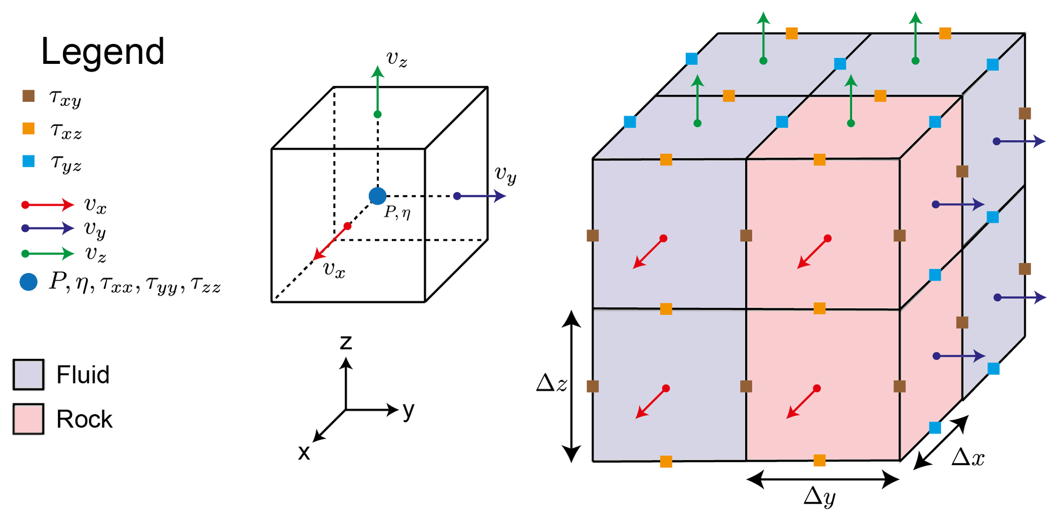
Pressures are defined in the middle of the staggered grid cell, whereas velocities are defined on cell faces. Based on the data from CT scans, each cell is assigned either a fluid or a solid phase. The discretized system is then solved using an iterative multigrid scheme to obtain values for velocities v and pressure P. To this end, we employ multigrid solvers which are part of the Portable, Extensible Toolkit for Scientific Computation (PETSc) library (Balay et al., 2010). As only cells belonging to the fluid phase exhibit non-zero values for the velocity, the velocity components belonging to solid cells are directly set to zero and only considered as boundary conditions. This greatly reduces the degrees of freedom of the system to be solved and hence also the computational cost. Pressures are fixed on the top and bottom boundaries and free-slip boundary conditions are employed on the side boundaries. As described above, no-slip boundary conditions apply at the solid–fluid interface. To solve the linear system of equations, a V-cycle geometric multiplicative multigrid solver is used (Fedorenko, 1964; Wesseling, 1995). The multigrid solver operates on up to five multigrid levels depending on the given input model. Convergence criteria are given by a relative convergence tolerance of 10−8 and an absolute convergence tolerance of 10−10 (see Appendix A1). The absolute convergence tolerance “atol” is defined as the absolute size of the residual norm and “rtol” the decrease of the residual norm relative to the norm of the right-hand side. Therefore, convergence at iteration k is reached for
where , with b the right-hand-side vector, x the solution vector of the current time step k and C the matrix representation of a linear operator (Balay et al., 2010).
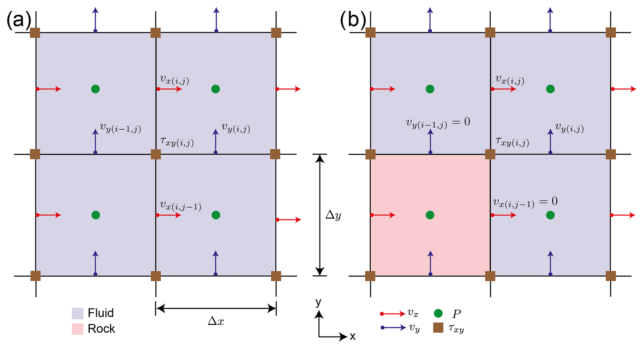
Assigning solid and fluid phases to different cells defines the location of the fluid–solid interface. In the case of a staggered grid, the location of the interface therefore does not correspond to the location of the interface-parallel velocity component. To illustrate this issue, the discretization stencil of a shear stress component τxy is shown in Fig. 2. When no interfaces are present (Fig. 2a), the finite different discretization results in the following expression (k index is omitted for brevity):
When stencils contain rock cells (e.g., Fig. 2b), we can straightforwardly enforce the no-flow conditions at their boundaries:
to obtain
This form, however, does not enforce interface-parallel velocities to be zero at the interface locations, which results in sub-optimal convergence. Alternatively, the exact constraints can be enforced:
which will give
The specific expression will depend on the exact subset of cells occupied by rock. The discretization of the other components is performed in a similar manner. The above modification of the shear stress discretization stencil is called here “stencil rescaling”. Similar approaches have already been presented in the literature (Vasilyev et al., 2016; Mostaghimi et al., 2013; Manwart et al., 2002). Both Manwart et al. (2002) and Mostaghimi et al. (2013) presented tests to validate their method. The test performed in Manwart et al. (2002) (permeability of a cubic array of spheres) exhibits non-monotonous convergence of the numerical solution. Mostaghimi et al. (2013) validated their method by comparing the numerical solution to the analytical solution of flow between two parallel plates. They found that they were able to compute the velocity “to within machine accuracy” if they used more than two grid cells but did not provide any information about convergence of the effective permeability.
To verify the method presented above, we performed a series of benchmark tests where we compared numerical solutions of simplified model setups to their respective analytical solutions. For simplicity, we non-dimensionalized the governing Eqs. (2) and (3) as well as the rheology given in Eq. (7) with characteristic values for viscosity ηc, length lc, stress τc and velocity vc:
where the characteristic value for vc can be derived from the other characteristic values. Non-dimensional values are denoted with a ∼. For the remainder of this section, we will only use non-dimensional values and drop the ∼ for simplicity. Benchmark tests are organized as follows: first, we will present three benchmark tests for the flow of a Newtonian fluid through (i) a single tube, (ii) multiple tubes and (iii) through a simple cubic sphere pack, which is followed by a benchmark test of power-law fluid flow through a single tube. The difference between numerically and analytically computed permeabilities is then expressed using the L2 norm of their relative misfit:
where kcomp is the computed and kana the analytically obtained permeability.
4.1 Newtonian flow through a single vertical tube
For a single vertical tube, the analytical solutions for both velocity v and flow rate Q are given as (e.g., Poiseuille, 1846; Landau and Lifshitz, 1987)
where is the pressure drop in the z direction, R the radius of the pipe and r the integration variable. The characteristic scales in this case are given by ηc=η0, τc=ΔP and lc=R, so that the pipe radius R, fluid viscosity η and pressure difference ΔP all take values of 1. The cubic model domain has an edge length of four units. Combining Eq. (21) with Eq. (4), the non-dimensional permeability is then given by
To assess the effect of different spatial resolutions, we conduct a resolution test where we increase resolution from 83 to 2563 nodes with a constant grid spacing in each direction. Four sets of resolution tests were conducted. In the first two sets, permeability was computed using the standard finite difference approach without stencil rescaling. The two sets then differ due to the exact location of the pipe. In set 1, the location of the pipe was chosen in such a way that the pipe surface aligned with the numerical grid (standard, ON NODE) so that computational nodes were directly located on the fluid–solid interface in the x and y directions. In set 2 (standard, OFF NODE), the location of the pipe was shifted so that the fluid–solid interface was located between the respective computational nodes. The same procedure was applied to sets 3 and 4 where stencil rescaling was employed. The reason to do that was to determine the effect of well-aligned computational nodes, as this is often not the case in more complex geometries.
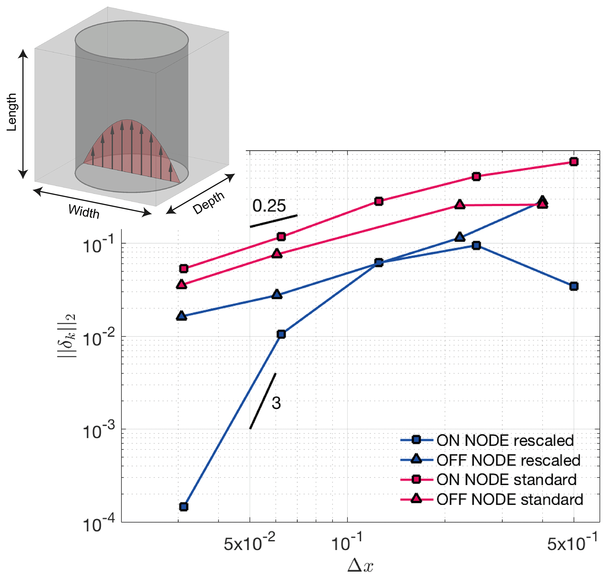
Figure 3Hagen–Poiseuille benchmark results. Shown is the error norm vs. spatial resolution. The different curves show cases where the tube surface coincides with a nodal point (ON NODE) or not (OFF NODE). Blue lines represent simulations using stencil rescaling, whereas red lines denote simulations without stencil rescaling. To highlight convergence, black lines with given slopes were added.
As expected, the numerical results generally show higher accuracy when stencil rescaling is employed and when node locations and interfaces of the tube are aligned (see Fig. 3). The order of convergence is linear for cases without rescaling or when the tube interface does not coincide with grid nodes but superlinear if both rescaling is employed and interface and node location coincide.
4.2 Newtonian flow through multiple vertical tubes
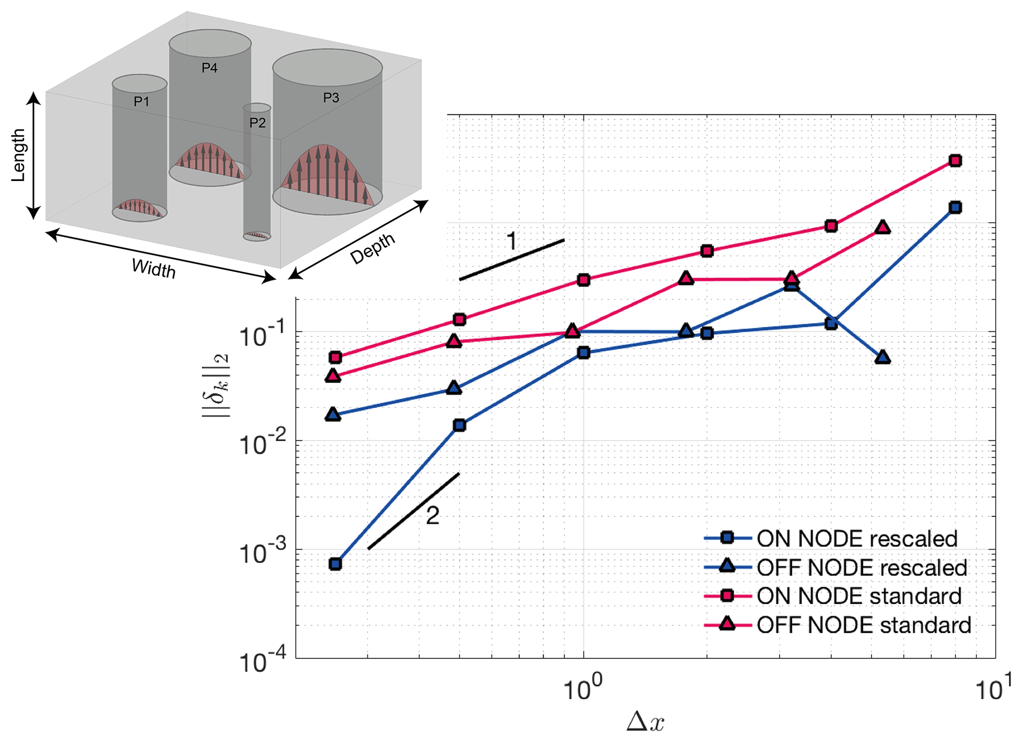
In natural rocks, larger channels tend to dominate the overall permeability. To assess this effect, we compute the flow through several straight tubes with different radii (Fig. 4). We use four pipes with non-dimensional radii given as R1=2, R2=1, R3=8, R4=4. The viscosity of the fluid is 1 and edge length of the cubic domain is 8. The simulations are performed in a similar manner to the single-tube benchmark by increasing the number of grid points from 83 to 2563. For each tube, the analytical solution (Eqs. 20, 21) is computed and the cumulative analytical permeability value is compared against computed values. The non-dimensional permeability in this case reads as
The individual tubes contribute to the absolute permeability as follows: P1=0.3662 %, P2=0.0229 %, P3=93.7514 %, P4=5.8595 %.
Similar to what was observed for the single-tube setup, the results show a lower relative error for calculations employing the stencil rescaling compared to those without. Furthermore, as shown for the setups with a single tube, the results are more accurate in cases where the numerical grid aligns with the tube surface. As expected, the overall permeability is dominated by the largest tube, as we do not see any significant changes within the relative error of the computed permeability.
4.3 Newtonian flow through simple cubic (SC) sphere packs
In order to verify the code for more complex geometries such as the vertical tube, we here consider simple cubic (SC) sphere packs. Sphere packs provide a geometry for different packings, as the porous medium is homogeneous. The setup has dimensions of 2 in all directions.
The permeability of an SC sphere pack is given by Sangani and Acrivos (1982) and Bear (1988):
where dsp is the sphere diameter and ϕ is the porosity for simple cubic packing of , respectively.
Figure 5 shows the increase in accuracy with increasing number of grid points employed. The presented relative errors of the permeability value are computed in the same manner as shown in Eq. (19). The simulations employing stencil rescaling show a better convergence and seem to saturate against a relative error of 10−1, demonstrating the influence of boundary effects through applied no-slip boundary conditions (finite size effect).
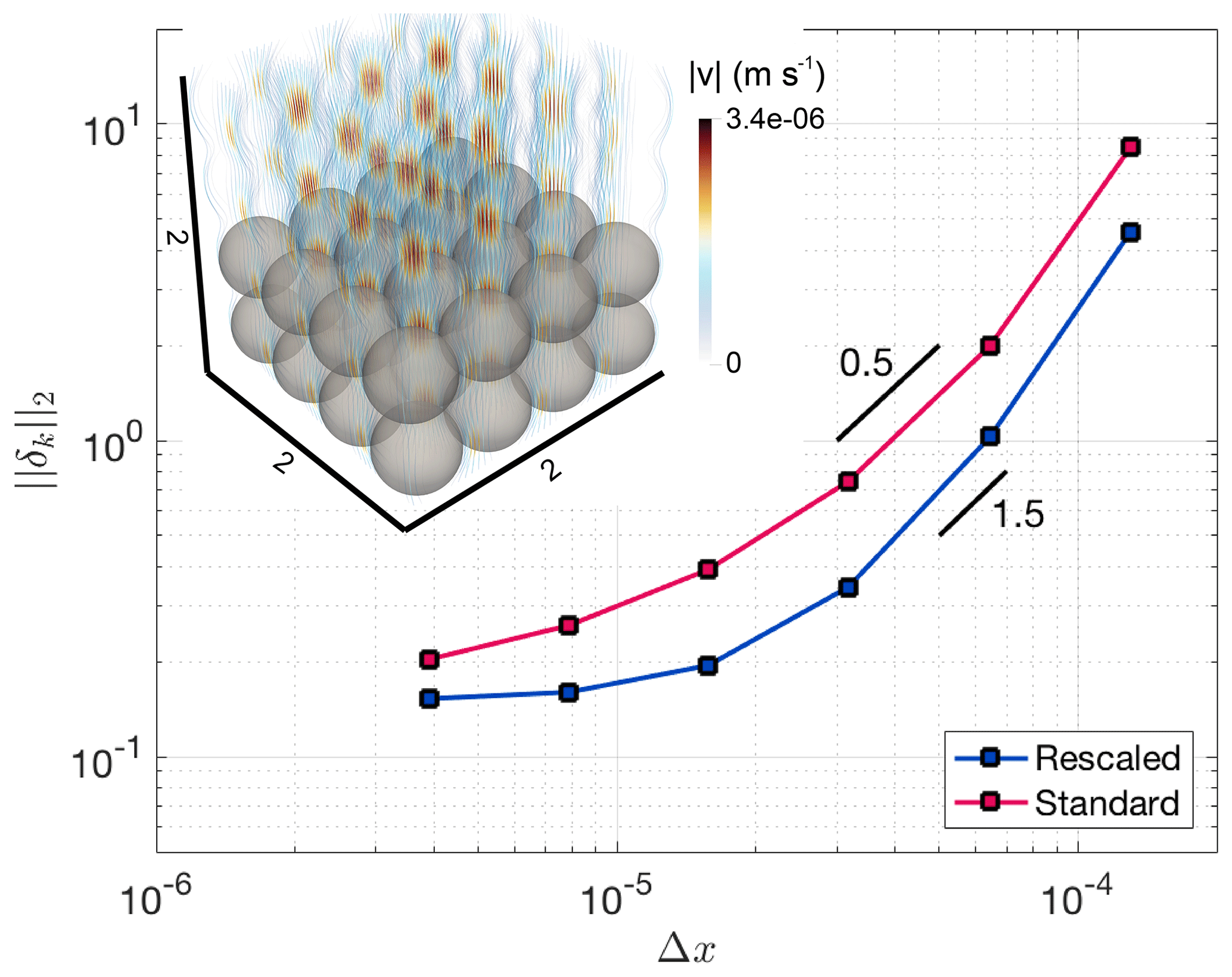
Figure 5Computed norm of the misfit between analytically and numerically computed permeabilities. The inset shows the discretization using four spheres in each direction (64 spheres in total). Streamlines are computed around those spheres and colorized with the computed velocity. Blue dots show results using stencil rescaling and red dots results with the standard method. To highlight convergence, black lines with given slopes were added.
4.4 Power-law fluid flow through a single vertical tube
In order to verify the computed value, we compare this setup against an analytical solution of Hagen–Poiseuille flow with power-law fluid behavior. For the single-tube configuration described in Sect. 4.1 and a power-law rheology, the velocity within the tube is given by, e.g., Turcotte and Schubert (2002):
where (see Appendix B), R is the tube radius and r the width of the tube in Cartesian coordinates. Figure 6 shows a good agreement between the numerical and analytical velocities for non-Newtonian fluids when using 0.5 and 2 as values for the power-law exponents, covering most fluids used for enhanced oil recovery (e.g., Najafi et al., 2017; Xie et al., 2018).

Figure 6Comparison of analytical and numerical velocities for Hagen–Poiseuille flow with a power-law fluid. Analytical velocities are represented as colored lines and numerical velocities as colored symbols.
To verify the ability of the code to handle more complex flows through natural samples and to validate previously computed permeability values, we used the CT data for a Fontainebleau sandstone sample provided by Andrä et al. (2013b) with dimensions 2.16 mm × 2.16 mm × 2.25 mm (resolved with 288 × 288 × 300 grid points). In order to optimize the computation and reduce computational resources, a subsample with dimensions of 2563 is used for further computations. The sample mainly consists of monodisperse quartz sand grains and is therefore a very popular sample for numerical and experimental permeability measurements. Furthermore, sandstone is known to be an ideal reservoir rock and is of certain interest for several geological fields, especially in exploration geology. Laboratory measurements of the given sample with porosity ≈15.2 % result in a permeability value of ≈1100 mD (Keehm, 2003).
5.1 Newtonian flow
As in previous tests, we compute the permeability of the extracted subsample using Eqs. (4) and (5). Figure 7a shows streamlines colored using computed fluid velocities and Fig. 7b the local pressure.
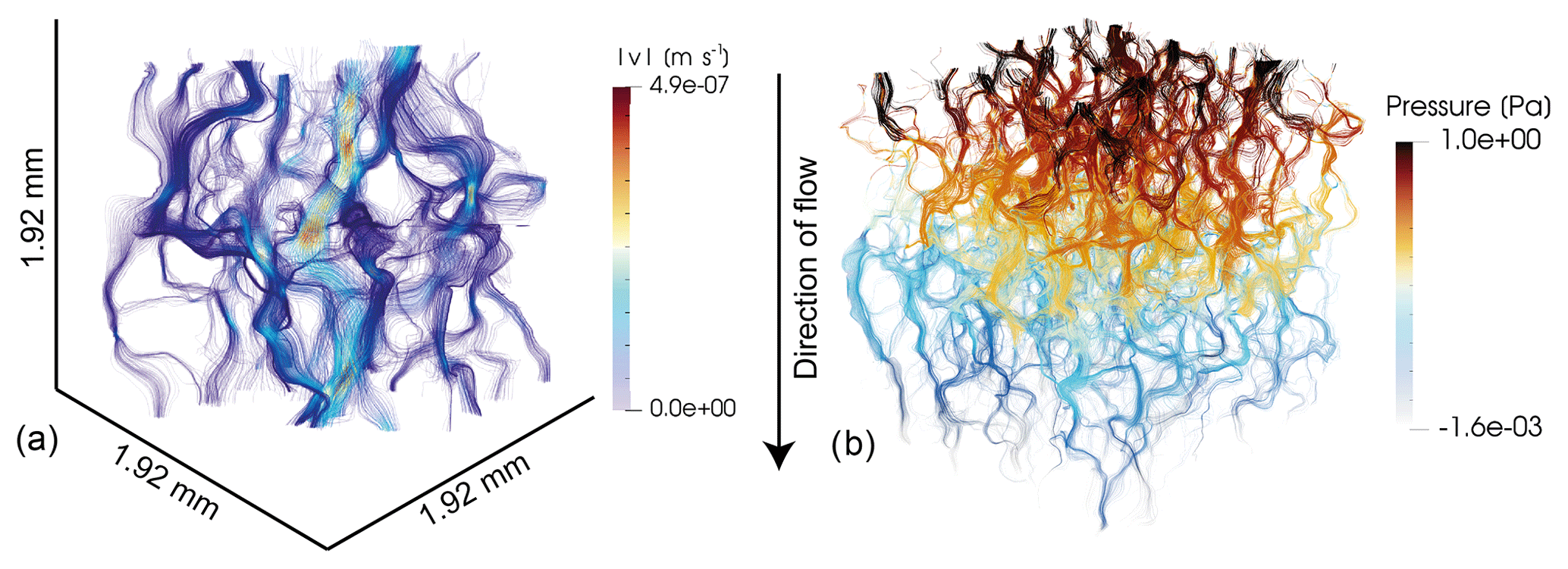
Figure 7Newtonian fluid flow through the Fontainebleau sandstone sample. Streamlines colored using computed fluid velocities are shown in panel (a) and streamlines colored using fluid pressures are shown in panel (b).
For a resolution of 2563, we obtain permeabilities which are comparable to previously computed permeabilities of the same sample (Fig. 8; Andrä et al., 2013b), with the rescaled stencil method yielding significantly lower values at higher resolutions. As previous tests show, permeabilities may be overestimated at lower resolutions. To test this effect, we increased the resolution of the Fontainebleau subsample by a factor of 2, 3 and 4 (5123, 7683, 10243). The resolution increase is achieved by subdividing a voxel into 2, 3 or 4 voxels. We do not apply any interpolation or stochastic reconstructions to conserve spacial statistics, as discussed by Karsanina and Gerke (2018). Determining the effects of these more sophisticated methods on computed permeabilities will require further work in the future. Figure 8 shows a comparison between the computed and measured values for the given Fontainebleau dataset. With increasing resolution of the subsample, the computed permeability value converges to the laboratory value. In comparison to the initial resolution of 2563, the computed permeability values decreased by ≈24.6 % when using a grid resolution of 10243. Additionally, the benefit of stencil rescaling can also be seen here, as, e.g., the simulation with a resolution of 5123 and stencil rescaling predicts nearly the same permeability as the case with doubled resolution and no stencil rescaling. Clearly, the models converge to a value that is close to the measured value. The numerical convergence is computed for several subsamples (see Appendix C). Figure 8 shows the convergence of a single subsample. Previous studies have also observed this convergence with increasing resolution, albeit not always from above (e.g., Zakirov and Galeev, 2019). Similar behavior has also been observed in Lattice–Boltzmann method (LBM) simulations (e.g., Khirevich et al., 2015; Khirevich and Patzek, 2018).
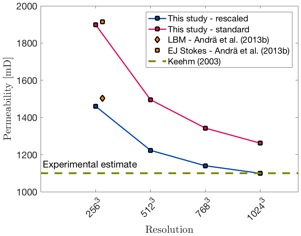
Figure 8Computed permeability values against grid resolution. Orange symbols denote simulations using Lattice–Boltzmann method (LBM) and explicit jump Stokes (EJ Stokes); both methods are used in Andrä et al. (2013b). Blue data points represent simulations using stencil rescaling, while simulations represented by red dots use the standard method. The brown dotted line symbolizes the experimental estimate from Keehm (2003).
5.2 Power-law fluid flow
To demonstrate the capability of the code to compute the flow of non-Newtonian fluids through porous media, we computed the average flow velocity vm for a square subsample of the Fontainebleau sandstone sample described above using the power-law rheology given in Eq. (7). The edge length of the subsample was 1.92 mm, which corresponds to a CT resolution of 2563 voxels. To increase accuracy, we increased this resolution by a factor of 2 to a resolution 5123. As seen in Sect. 5.1, results at this resolution may overestimate the actual permeability value. The chosen resolution thus represents a compromise between accuracy and computational cost. The reference viscosity was set to η0=1 Pa and η1 and η2 were set to 10−3 and 106, respectively. Two sets of simulations using a power-law exponent of 0.5 and 1 were performed. In each set, the applied pressure at the top boundary is changed from 1 to 16 Pa. In Fig. 9, we plot the applied pressure at the top boundary against the computed average velocity. For both sets of simulations, the computed slopes of and are in good agreement with the imposed power-law coefficients of 0.5 and 1 (Eq. 8).
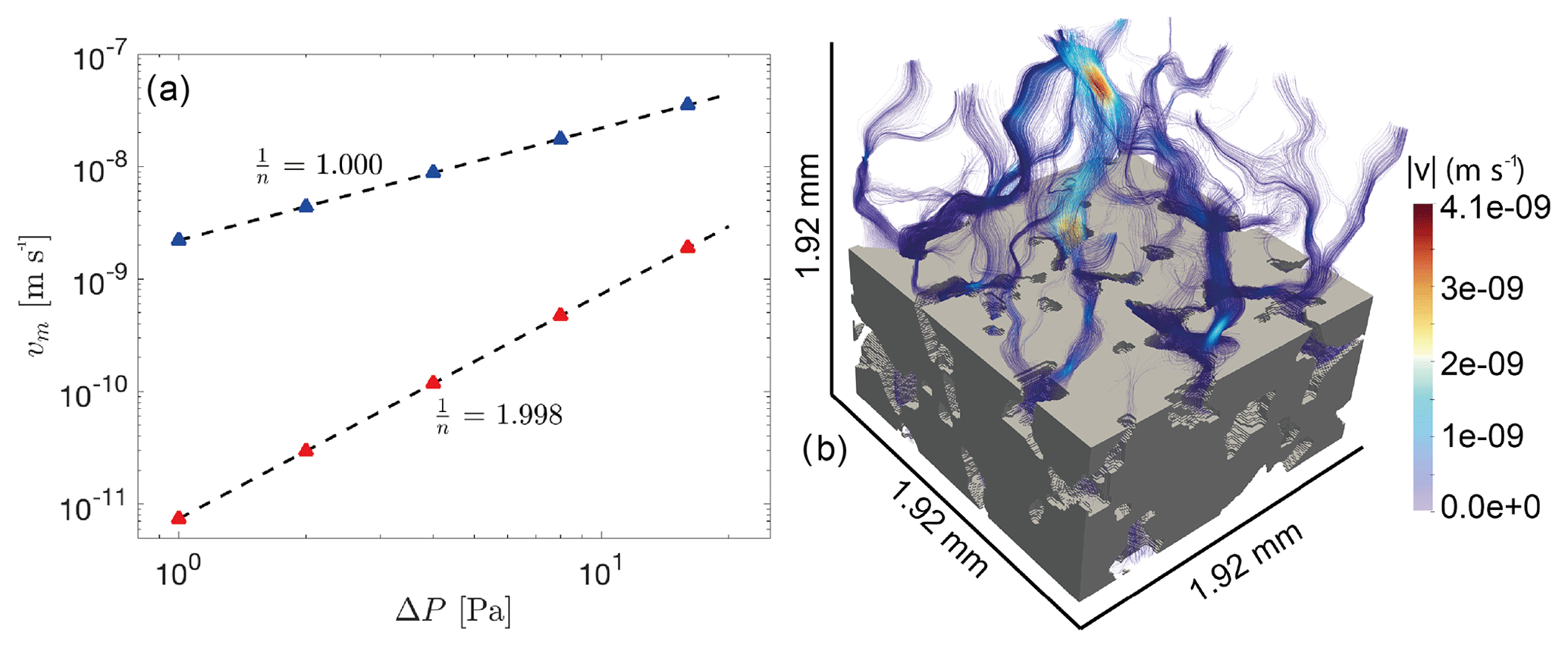
Figure 9Computed results on the Fontainebleau sample using non-Newtonian rheology. Panel (a) shows the mean velocity against the applied pressure at the top boundary. Red and blue triangles symbolize each simulation, and the corresponding dotted black line represents the fitted curve through the obtained data with slope . Panel (b) illustrates computed streamlines of the Fontainebleau subsample using a power-law coefficient of 0.5. Solid material is displayed in grey and the streamlines are colored according to computed velocities.
In this paper, we presented the capability of the open-source finite difference solver LaMEM to compute the permeability of given porous media. The code was verified using a set of benchmark problems with given analytical solutions ranging from Hagen–Poiseuille flow through vertical tubes to more complex flow through simple cubic sphere packs. Using CT data of a Fontainebleau sandstone, we then demonstrated that the code is able to predict the permeability of natural porous media. In both benchmarks and application tests, the benefits of the stencil rescaling method can be observed, as this method provides significantly more accurate results at no additional computational cost.
Benchmarking results for single and multiple tubes demonstrate that the permeability calculation improves considerably in the case that the fluid–solid interface and the numerical grid are at least partially aligned. Cases using the stencil rescaling solutions with a velocity change on a computational node produce smaller relative errors.
Similar to studies using the LBM (Knackstedt and Zhang, 1994; Zhang et al., 2000; Keehm, 2003), our resolution test for the Fontainebleau subsample shows that the computed permeability value also decreases with increasing grid resolution. For instance, computing the permeability of the Fontainebleau sandstone sample with grid resolution of 10243, calculations employing stencil rescaling give approximately the same permeability value as suggested by laboratory measurements, while simulations without employing stencil rescaling overestimate the computed permeability by ≈14.72 %. (Fig. 8). However, this behavior may also be the opposite depending on the numerical implementation of the respective numerical method (e.g., Khirevich et al., 2015; Khirevich and Patzek, 2018; Zakirov and Galeev, 2019).
The computation of permeabilities in a three-dimensional pore space using micro-CT data strongly depends on the reasonable quality of the micro-CT images followed by several steps of segmentation in order to resolve tiny fluid pathways. Although high-quality input data are required in most cases, it is usually computationally expensive to use the entire micro-CT scan with full resolution; thus, representative subvolumes or a reduced numerical resolution have to be used, as computational resources are limited.
Additionally, the segmentation of the CT data has a considerable effect on the computed permeability, as discussed in Andrä et al. (2013a), since segmentation of the acquired micro-CT data has a major effect on the three-dimensional pore space and therefore on the obtained value. In two-phase systems (fluid–solid), segmentation is straightforward, whereas it may become more difficult in multiphase systems. All of the above points are a source of uncertainty and need to be considered when comparing numerical calculations to laboratory measurements for rock samples. Furthermore, we showed that LaMEM is able to compute non-Newtonian fluid flow in porous media, which is not only relevant for geosciences but also of importance for industrial applications (Saidur et al., 2011).
Furthermore, it should be kept in mind that solver options like convergence criteria may influence the obtained permeability result. Figure A1 (see Appendix A) highlights the effect of different relative tolerances on the computed permeability value. In order to avoid spurious results, we recommend to test the influence of the relative and absolute tolerance on the model outcome.
The simulations were performed on the clusters of University of Bayreuth and University of Mainz using different numbers of CPUs depending on the size of the computed domain. As an example, a simulation with 5123 voxels uses 1024 CPUs, 185 GB RAM and requires 5790 s computation time. Apart from LaMEM, finite difference codes like FDMSS (Gerke et al., 2018) compute permeability of porous media more efficient, but these codes mostly are not able to compute fluid flow using non-linear viscosity.
In conclusion, the capability of the open-source finite difference solver LaMEM to accurately simulate Newtonian and non-Newtonian fluid flow in porous media is successfully demonstrated for different setups with an increasing geometric complexity including pipe flow, ordered sphere packs and a micro-CT dataset of Fontainebleau sandstone.
The code used to produce this results is available at https://bitbucket.org/bkaus/lamem/src/master/ (Popov and Kaus, 2016); commit no: 676374f.
To determine whether a numerical solution converges, two convergence criteria, which are absolute and relative convergence tolerance, are used. To test the effect on the numerical solution, we varied both while computing permeability of three different setups. Our results show that the obtained permeability value saturates for relative convergence tolerances . Thus, for all further simulations, a relative convergence tolerance of 10−8 is used (Fig. A1). A change in the absolute convergence tolerance did not have any effect on the computed solution; therefore, we use an absolute convergence tolerance of 10−10.

Figure A1Results of simulations for (a) Hagen–Poiseuille single tube, (b) simple cubic sphere pack and (c, d) Fontainebleau sandstone using different relative/absolute convergence tolerances.
C1 is an constant arising during the derivation of Eq. (25), which is related to the non-linear rheology used in Turcotte and Schubert (2002). This rheology is written as
where n′ is the stress exponent as used for power-law materials in geodynamics. Replacing τ with leads to
Solving Eq. (B2) for η results in
We can now define a reference viscosity η0 at a reference strain rate . This reference viscosity then reads as
Assuming and solving for C1 then provides us with the following expression:
In order to show numerical convergence of the given Fontainebleau sample, several subsamples were extracted and the resolution increased to 5123, 7683 and 10243 grid points. Figure C1 displays the convergence with increasing grid resolution. The different subsamples show a variance of around 12 % for the computed permeability value.
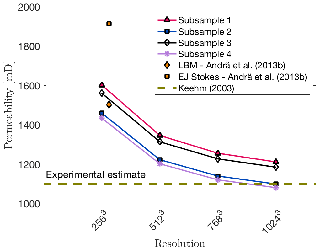
Figure C1Numerical convergence of different Fontainebleau subsamples with increasing grid resolution. All subsamples displayed were computed using stencil rescaling. For comparison, the computed permeabilities from Andrä et al. (2013b) are shown. The dotted brown line symbolizes the experimental estimate taken from Keehm (2003).
PE did the bulk of the work, including writing, visualization, methodology and running simulations. MT and GJG designed the study and contributed to manuscript writing. AP implemented stencil rescaling into LaMEM. WF assisted in code benchmarking. MOK performed the resolution test for Fontainebleau subsamples. BJPK contributed to data interpretation and manuscript writing.
The authors declare that they have no conflict of interest.
This work was founded by DFG (grant no. GRK 2156/1) and the BMBF (grant no. 03G0865A). Marcel Thielmann has received funding from the Bayerisches Geoinstitut Visitors Program. Simulations were performed on the btrzx2 cluster, University of Bayreuth, and the Mogon II cluster, Johannes Gutenberg University, Mainz. We would like to thank Kirill Gerke and Stéphane Beaussier for their constructive reviews that helped to improve the manuscript.
This research has been supported by the Deutsche Forschungsgemeinschaft (grant no. GRK 2156/1) and the Bundesministerium für Bildung und Forschung (grant no. 03G0865A).
This open-access publication was funded
by the University of Bayreuth.
This paper was edited by Patrice Rey and reviewed by Kirill Gerke and Stephane Beaussier.
Aharonov, E. and Rothman, D. H.: Non-Newtonian flow (through porous media): A lattice-Boltzmann method, Geophys. Res. Lett., 20, 679–682, 1993. a
Akanji, L. T. and Matthai, S. K.: Finite element-based characterization of pore-scale geometry and its impact on fluid flow, Transport Porous Med., 81, 241–259, 2010. a
Andrä, H., Combaret, N., Dvorkin, J., Glatt, E., Han, J., Kabel, M., Keehm, Y., Krzikalla, F., Lee, M., Madonna, C., Marsh, M., Mukerji, T., Saenger, E. H., Sain, R., Saxena, N., Ricker, S., Wiegmann, A., and Zhan, X.: Digital rock physics benchmarks – Part I: Imaging and segmentation, Comput. Geosci., 50, 25–32, 2013a. a
Andrä, H., Combaret, N., Dvorkin, J., Glatt, E., Han, J., Kabel, M., Keehm, Y., Krzikalla, F., Lee, M., Madonna, C., Marsh, M., Mukerji, T., Saenger, E. H., Sain, R., Saxena, N., Ricker, S., Wiegmann, A., and Zhan, X.: Digital rock physics benchmarks – Part II: Computing effective properties, Comput. Geosci., 50, 33–43, 2013b. a, b, c, d, e
Arns, C. H.: A comparison of pore size distributions derived by NMR and X-ray-CT techniques, Physica A: Statistical Mechanics and its Applications, Proceedings of the International Conference New Materials and Complexity, 339, 159–165, 2004. a
Arns, C. H., Knackstedt, M. A., Pinczewski, M. V., and Lindquist, W.: Accurate estimation of transport properties from microtomographic images, Geophys. Res. Lett., 28, 3361–3364, 2001. a
Balay, S., Buschelman, K., Eijkhout, V., Gropp, W., Kaushik, D., Knepley, M., Mcinnes, L. C., Smith, B., and Zhang, H.: PETSc Users Manual, ReVision, 2, 1–211, 2010. a, b
Bear, J.: Dynamics of Fluids in Porous Media, Dover Publications Inc., New York, Reprint, p. 764, 1988. a, b
Bird, R. B., Lightfoot, E. N., and Stewart, W. E.: Transport Phenomena, New York, London, 1960. a, b, c
Bird, M., Butler, S. L., Hawkes, C., and Kotzer, T.: Numerical modeling of fluid and electrical currents through geometries based on synchrotron X-ray tomographic images of reservoir rocks using Avizo and COMSOL, Comput. Geosci., 73, 6–16, 2014. a
Bosl, W. J., Dvorkin, J., and Nur, A.: A study of porosity and permeability using a lattice Boltzmann simulation, Geophys. Res. Lett., 25, 1475–1478, 1998. a, b, c
Brace, W.: Permeability of crystalline and argillaceous rocks, Int. J. Rock Mech. Min., Elsevier, 17, 241–251, 1980. a
Brace, W.: Permeability of crystalline rocks: New in situ measurements, J. Geophys. Res.-Sol. Ea., 89, 4327–4330, 1984. a
Carman, P. C.: Fluid flow through granular beds, Trans. Inst. Chem. Eng., 15, 150–166, 1937. a
Carman, P. C.: Flow of gases through porous media, New York, Academic Press, 182 pp., 1956. a
Cassidy, M., Manga, M., Cashman, K., and Bachmann, O.: Controls on explosive-effusive volcanic eruption styles, Nat. Commun., 9, 1–16, 2018. a
Choi, S. U.: Nanofluids: from vision to reality through research, J. Heat Transf., 131, 033106, https://doi.org/10.1115/1.3056479, 2009. a
Cui, X., Bustin, A., and Bustin, R. M.: Measurements of gas permeability and diffusivity of tight reservoir rocks: different approaches and their applications, Geofluids, 9, 208–223, 2009. a
Deubelbeiss, Y., Kaus, B. J. P., Connolly, J. A. D., and Caricchi, L.: Potential causes for the non-Newtonian rheology of crystal-bearing magmas, Geochem. Geophy. Geosy., 12, Q05007, https://doi.org/10.1029/2010GC003485, 2011. a
Diersch, H.-J. G.: FEFLOW: finite element modeling of flow, mass and heat transport in porous and fractured media, Springer Science & Business Media, 996 pp., 2013. a
Dikinya, O., Hinz, C., and Aylmore, G.: Decrease in hydraulic conductivity and particle release associated with self-filtration in saturated soil columns, Geoderma, 146, 192–200, 2008. a
Dvorkin, J., Derzhi, N., Diaz, E., and Fang, Q.: Relevance of computational rock physics, Geophysics, 76, E141–E153, 2011. a
Fedorenko, R. P.: The speed of convergence of one iterative process, J. Comput. Math. Math. Phys., 4, 227–35, 1964. a
Fehn, U. and Cathles, L. M.: Hydrothermal convection at slow-spreading mid-ocean ridges, Tectonophysics, 55, 239–260, 1979. a
Ferland, P., Guittard, D., and Trochu, F.: Concurrent methods for permeability measurement in resin transfer molding, Polym. Composites, 17, 149–158, 1996. a
Ferreol, B. and Rothman, D. H.: Lattice-Boltzmann simulations of flow through Fontainebleau sandstone, in: Multiphase flow in porous media, Springer, 3–20, 1995. a
Fredrich, J., Greaves, K., and Martin, J.: Pore geometry and transport properties of Fontainebleau sandstone, Int. J. Rock Mech. Min., Elsevier, 30, 691–697, 1993. a
Garcia, X., Akanji, L. T., Blunt, M. J., Matthai, S. K., and Latham, J. P.: Numerical study of the effects of particle shape and polydispersity on permeability, Phys. Rev. E, 80, 021304, https://doi.org/10.1103/PhysRevE.80.021304, 2009. a
Gerke, K. M., Sidle, R. C., and Mallants, D.: Preferential flow mechanisms identified from staining experiments in forested hillslopes, Hydrol. Process., 29, 4562–4578, 2015. a
Gerke, K. M., Vasilyev, R. V., Khirevich, S., Collins, D., Karsanina, M. V., Sizonenko, T. O., Korost, D. V., Lamontagne, S., and Mallants, D.: Finite-difference method Stokes solver (FDMSS) for 3D pore geometries: Software development, validation and case studies, Comput. Geosci., 114, 41–58, 2018. a, b
Glazner, A. F.: Magmatic life at low Reynolds number, Geology, 42, 935–938, https://doi.org/10.1130/G36078.1, 2014. a
Guo, Z. and Zhao, T.: Lattice Boltzmann model for incompressible flows through porous media, Phys. Rev. E, 66, 036304, https://doi.org/10.1103/PhysRevE.66.036304, 2002. a
Harlow, F. H. and Welch, J. E.: Numerical calculation of time-dependent viscous incompressible flow of fluid with free surface, Phys. Fluids, 8, 2182–2189, 1965. a
Huang, Y., Yang, Z., He, Y., and Wang, X.: An overview on nonlinear porous flow in low permeability porous media, Theor. Appl., 3, 022001, https://doi.org/10.1063/2.1302201, 2013. a
Johnston, B. M., Johnston, P. R., Corney, S., and Kilpatrick, D.: Non-Newtonian blood flow in human right coronary arteries: steady state simulations, J. Biomech., 37, 709–720, 2004. a
Karsanina, M. V. and Gerke, K. M.: Hierarchical Optimization: Fast and Robust Multiscale Stochastic Reconstructions with Rescaled Correlation Functions, Phys. Rev. Lett., 121, 265501, https://doi.org/10.1103/PhysRevLett.121.265501, 2018. a
Kaus, B. J. P., Popov, A. A., Baumann, T. S., E, P. A., Bauville, A., Fernandez, N., and Collignon, M.: Forward and Inverse Modelling of Lithospheric Deformation on Geological Timescales, NIC Series, 48, 978–3, 2016. a
Keehm, Y.: Computational rock physics: Transport properties in porous media and applications, Ph.D. thesis, Stanford University, 135 pp., 2003. a, b, c, d, e, f
Khirevich, S. and Patzek, T. W.: Behavior of numerical error in pore-scale lattice Boltzmann simulations with simple bounce-back rule: Analysis and highly accurate extrapolation, Phys. Fluids, 30, 093604, https://doi.org/10.1063/1.5042229, 2018. a, b
Khirevich, S., Ginzburg, I., and Tallarek, U.: Coarse- and fine-grid numerical behavior of MRT/TRT lattice-Boltzmann schemes in regular and random sphere packings, J. Comput. Phys., 281, 708–742, 2015. a, b
Knackstedt, M. and Zhang, X.: Direct evaluation of length scales and structural parameters associated with flow in porous media, Phys. Rev. E, 50, 2134, https://doi.org/10.1103/PhysRevE.50.2134, 1994. a
Knackstedt, M. A., Latham, S., Madadi, M., Sheppard, A., Varslot, T., and Arns, C.: Digital rock physics: 3D imaging of core material and correlations to acoustic and flow properties, The Leading Edge, 28, 28–33, 2009. a
Kozeny, J.: Über kapillare Leitung des Wassers im Boden, Royal Academy of Science, Vienna, Proc. Class I, 136, 271–306, 1927. a
Landau, L. D. and Lifshitz, E. M.: Course of theoretical physics. vol. 6: Fluid mechanics, Pergamon Press, p. 539, 1987. a
Larson, R. G.: Derivation of generalized Darcy equations for creeping flow in porous media, Ind. Eng. Chem. Fund., 20, 132–137, 1981. a
Mader, H. M., Llewellin, E. W., and Mueller, S. P.: The rheology of two-phase magmas: A review and analysis, J. Volcanol. Geoth. Res., 257, 135–158, 2013. a, b
Manwart, C., Aaltosalmi, U., Koponen, A., Hilfer, R., and Timonen, J.: Lattice-Boltzmann and finite-difference simulations for the permeability for three-dimensional porous media, Phys. Rev. E, 66, 016702, https://doi.org/10.1103/PhysRevE.66.016702, 2002. a, b, c, d, e
Mavko, G. and Nur, A.: The effect of a percolation threshold in the Kozeny-Carman relation, Geophysics, 62, 1480–1482, 1997. a
Mostaghimi, P., Blunt, M. J., and Bijeljic, B.: Computations of absolute permeability on micro-CT images, Math. Geosci., 45, 103–125, 2013. a, b, c, d
Najafi, S. A. S., Kamranfar, P., Madani, M., Shadadeh, M., and Jamialahmadi, M.: Experimental and theoretical investigation of CTAB microemulsion viscosity in the chemical enhanced oil recovery process, J. Mol. Liq., 232, 382–389, 2017. a
Norton, D. and Taylor Jr., H.: Quantitative simulation of the hydrothermal systems of crystallizing magmas on the basis of transport theory and oxygen isotope data: An analysis of the Skaergaard intrusion, J. Petrol., 20, 421–486, 1979. a
Osorno, M., Uribe, D., Ruiz, O. E., and Steeb, H.: Finite difference calculations of permeability in large domains in a wide porosity range, Arch. Appl. Mech., 85, 1043–1054, 2015. a
Pan, C., Hilpert, M., and Miller, C.: Lattice-Boltzmann simulation of two-phase flow in porous media, Water Resour. Res., 40, W01501, https://doi.org/10.1029/2003WR002120, 2004. a
Poiseuille, J. L.: Experimental research on the movement of liquids in tubes of very small diameters, Mémoires presentés par divers savants a l'Académie Royale des Sciences de l'Institut de France, IX, 433–544, 1846. a
Popov, A. and Kaus, B. J. P.: LaMEM, Lithosphere and Mantle Evolution Model, available at: https://bitbucket.org/bkaus/lamem/src/master/, BitBucket repository, BitBucket, commit no. 676374f, 2016. a
Sahimi, M. and Yortsos, Y. C.: Applications of fractal geometry to porous media, A review, Society of Petroleum Engineers, 25 pp., 1990. a
Saidur, R., Leong, K., and Mohammad, H.: A review on applications and challenges of nanofluids, Renewable and Sustainable Energy Reviews, 15, 1646–1668, 2011. a
Sangani, A. S. and Acrivos, A.: Slow flow through a periodic array of spheres, Int. J. Multiphas. Flow, 8, 343–360, 1982. a
Saxena, N. and Mavko, G.: Estimating elastic moduli of rocks from thin sections: digital rock study of 3D properties from 2D images, Comput. Geosci., 88, 9–21, 2016. a
Saxena, N., Mavko, G., Hofmann, R., and Srisutthiyakorn, N.: Estimating permeability from thin sections without reconstruction: Digital rock study of 3D properties from 2D images, Comput. Geosci., 102, 79–99, 2017. a, b
Shabro, V., Kelly, S., Torres-Verdín, C., Sepehrnoori, K., and Revil, A.: Pore-scale modeling of electrical resistivity and permeability in FIB-SEM images of organic mudrock, Geophysics, 79, D289–D299, 2014. a
Shah, C. and Yortsos, Y.: Aspects of flow of power-law fluids in porous media, AIChE J., 41, 1099–1112, 1995. a
Suleimanov, B. A., Ismailov, F., and Veliyev, E.: Nanofluid for enhanced oil recovery, J. Petrol. Sci. Eng., 78, 431–437, 2011. a
Turcotte, D. and Schubert, G.: Geodynamics, Cambridge Univ. Press, New York, 232 pp., 2002. a, b
Vakilha, M. and Manzari, M. T.: Modelling of power-law fluid flow through porous media using smoothed particle hydrodynamics, Transport Porous Med., 74, 331–346, 2008. a
Vasilyev, R. V., Gerke, K. M., Karsanina, M. V., and Korost, D. V.: Solution of the Stokes equation in three-dimensional geometry by the finite-difference method, Math. Model. Comput. Simul., 8, 63–72, 2016. a
Wasan, D. T. and Nikolov, A. D.: Spreading of nanofluids on solids, Nature, 423, 156–159, https://doi.org/10.1038/nature01591, 2003. a
Wesseling, P.: Introduction To Multigrid Methods, Institute for computer applications in science and engineering Hampton VA, Tech. Rep., 161, 683–691, https://doi.org/10.1016/j.petrol.2017.11.049, 1995. a
Xie, C., Lv, W., and Wang, M.: Shear-thinning or shear-thickening fluid for better EOR? – A direct pore-scale study, J. Petrol. Sci. Eng., 161, 683–691, 2018. a
Zakirov, T. and Galeev, A.: Absolute permeability calculations in micro-computed tomography models of sandstones by Navier-Stokes and lattice Boltzmann equations, Int. J. Heat Mass Tran., 129, 415–426, 2019. a, b
Zeinijahromi, A., Farajzadeh, R., Bruining, J. H., and Bedrikovetsky, P.: Effect of fines migration on oil–water relative permeability during two-phase flow in porous media, Fuel, 176, 222–236, 2016. a
Zhang, D., Zhang, R., Chen, S., and Soll, W. E.: Pore scale study of flow in porous media: Scale dependency, REV, and statistical REV, Geophys. Res. Lett., 27, 1195–1198, 2000. a
- Abstract
- Introduction
- Fluid flow in porous media
- Method
- Comparison with analytical solutions
- Application to Fontainebleau sandstone
- Discussion and conclusion
- Code availability
- Appendix A: Convergence criteria
- Appendix B: Definition of C1
- Appendix C: Permeabilities of different Fontainebleau subsamples
- Author contributions
- Competing interests
- Acknowledgements
- Financial support
- Review statement
- References