the Creative Commons Attribution 4.0 License.
the Creative Commons Attribution 4.0 License.
 | 21 Jan 2019
3-D seismic travel-time tomography validation of a detailed subsurface model: a case study of the Záncara river basin (Cuenca, Spain)
David Marti
Ignacio Marzan
Jana Sachsenhausen
Joaquina Alvarez-Marrón
Mario Ruiz
Montse Torne
Manuela Mendes
Ramon Carbonell
A high-resolution seismic tomography survey was acquired to obtain a full 3-D P-wave seismic velocity image in the Záncara river basin (eastern Spain). The study area consists of lutites and gypsum from a Neogene sedimentary sequence. A regular and dense grid of 676 shots and 1200 receivers was used to image a 500 m×500 m area of the shallow subsurface. A 240-channel system and a seismic source, consisting of an accelerated weight drop, were used in the acquisition. Half a million travel-time picks were inverted to provide the 3-D seismic velocity distribution up to 120 m depth. The project also targeted the geometry of the underground structure with emphasis on defining the lithological contacts but also the presence of cavities and fault or fractures. An extensive drilling campaign provided uniquely tight constraints on the lithology; these included core samples and wireline geophysical measurements. The analysis of the well log data enabled the accurate definition of the lithological boundaries and provided an estimate of the seismic velocity ranges associated with each lithology. The final joint interpreted image reveals a wedge-shaped structure consisting of four different lithological units. This study features the necessary key elements to test the travel time tomographic inversion approach for the high-resolution characterization of the shallow subsurface. In this methodological validation test, travel-time tomography demonstrated to be a powerful tool with a relatively high capacity for imaging in detail the lithological contrasts of evaporitic sequences located at very shallow depths, when integrated with additional geological and geophysical data.
- Article
(6952 KB) - Full-text XML
- BibTeX
- EndNote


Knowledge of the very shallow structure of the Earth has become a critical demand for modern society. The shallow subsurface is the part of the Earth with which humans have the most interaction. Characterizing the subsurface is important since it hosts critical natural resources; it is used as a reservoir for resources and waste, plays a key role in support of infrastructure planning, and holds the imprint of anthropogenic processes. Thus, understanding its composition and structure is a regular objective in studies such as natural resource exploration (Davis et al., 2003; Place et al., 2015) and environmental assessment studies (Steeples, 2001; Zelt et al., 2006). It is also critical in civil engineering and monitoring of underground structures (Escuder Viruete et al., 2003; Malehmir et al., 2007; Juhlin et al., 2007; Martí et al., 2008; Giese et al., 2009; Alcalde et al., 2013a). In addition, the implementation of a competent subsurface exploration scheme is very valuable for assessing and providing detailed site characterization for addressing natural hazards, e.g., seismic hazard (Samyn et al., 2012; Ugalde et al., 2013; Wadas et al., 2017; Bernal et al., 2018). Typical geotechnical practice for subsurface exploration has often relied on a combination of drilling, in situ testing, geophysical surveys and laboratory analysis of field samples (Andara et al., 2011; Kazemeini et al., 2010; Alcalde et al., 2014).
Geophysical techniques provide a great variety of approaches to accurately describe the structure and the distribution of different physical properties in the subsurface. Depending on the target depth and the required spatial resolution, different methodologies can be applied (e.g., Bryś et al., 2018; Novitsky et al., 2018; Malehmir et al., 2009 and 2011; Escuder Viruete et al., 2004; Carbonell et al., 2010; Ogaya et al., 2016; Andrés et al., 2016; Alcalde et al., 2013b). Since the late 90s, sophisticated geophysical techniques have been developed to estimate near-surface velocity models as a proxy for subsurface stiffness in seismic applications with different targets (Bergman et al., 2004 and 2006; Heincke et al., 2010). Seismic travel-time tomography is a robust, efficient and well contrasted tool to constrain the rock's physical properties at very shallow depths (Yordkayhun et al., 2009b; Flecha et al., 2004, 2006; Martí et al., 2002a; Baumann-Wilke et al., 2012). When seismic data are densely acquired it can provide very high spatial resolution images even in 3-D at a much more affordable cost than conventional 3-D seismic reflection surveys. In areas where the geology has no particularly internal structural complexity and with moderate lateral lithological variability, travel-time tomography can provide a reliable image of the subsurface (Martí et al., 2002b, 2006; Yordkayhun et al., 2009a; Letort et al., 2012; Baumann-Wilke et al., 2012)

Figure 1(a) Simplified geological map of the Iberian Chain in the eastern Iberian Peninsula, with the location of the study area marked by a black box (modified from Guimerà et al., 2004). (b) Local geological map of the Villar de Cañas syncline. The target area is marked by a blue rectangle. The 2-D seismic reflection profiles acquired in this experiment are also located in the map. (c) Detailed stratigraphic columns describing the main units observed in both flanks of the syncline.
The study area, in the Loranca Basin (Cuenca, Spain), has been considered as a possible host for a singular facility for temporary storage of radioactive waste. The emplacement of such a facility requires an extensive multiscale, multidisciplinary study of the site's subsurface (Witherspoon et al., 1981; IAEA, 2006; Kim et al., 2011), including a detailed 3-D distribution of its physical properties, especially focused on the upper 100 m that directly interacts with the ongoing construction works. The available data suggest that the sedimentary sequence in the study area presents certain tilting to the west, with no significant faulting and therefore no great structural complexity is expected in the shallow subsurface. Following similar case studies of very shallow characterization, travel-time tomography was used to provide constraints on the seismic velocities for the 3-D baseline model of the test site (Martí et al., 2002b; Juhlin et al., 2007; Yordkayhun et al., 2007).
A very dense source–receiver grid was designed to assure the necessary lateral resolution and depth coverage of the seismic data, and to constrain the geological features of interest beneath the construction site. The specific target was to build a 3-D distribution of the physical properties of a mostly gypsiferous succession with diffuse lithological boundaries (Martinius et al., 2002; Diaz-Molina and Muñoz-Garcia, 2010; Escavy et al., 2012). The inversion of almost half a million first arrival travel-time picks provided a detailed 3-D distribution of the P-wave velocities. This, combined with borehole information, allowed us to infer structural features, characterized by three main lithological units that constrained the interpretation of the velocity model. Borehole information was instrumental to define the specific 3-D geometry of the different lithologies in the tomographic model and the topography of the complex boundaries.
The area of Villar de Cañas (Cuenca, Spain) is included in the Loranca Basin, in the southwestern branch of the Iberian Chain (Fig. 1a). The Iberian Chain corresponds to a wide, mostly east-southeast-trending, Alpine intraplate orogen in the eastern Iberian Peninsula. The structure consists of a thin-skinned, west-verging, mostly imbricate thrust system and associated fault-propagation folds that deform a Mesozoic and Cenozoic sedimentary cover detached above the Paleozoic basement (Muñoz-Martín and De Vicente, 1998; Sopeña and De Vicente, 2004). The thrust faults merge at depth into a basal detachment located within Middle Triassic to Upper Triassic sequences (Piña-Varas el al., 2013).
The crustal structure of the Iberian Chain has gathered academic interest since the early 1990s (see Seillé et al., 2015; Guimerà et al., 2016, and references therein), including the acquisition of local and regional geologic and geophysical studies of the Loranca Basin (Biete et al., 2012; Piña-Varas et al., 2013). The Loranca Basin comprises syntectonic Cenozoic strata (Guimerà et al., 2004). It has been interpreted as a piggy-back basin that evolved during the Late Oligocene–Early Miocene period and includes mostly fluvial and lacustrine facies sediments, organized into three major alluvial fan sequences and their associated flooding plains (Díaz-Molina and Tortosa, 1996). The alluvial fans were fed from the southeastern and western boundaries of the basin and were comprised of mostly sandstones, gravels, mudstones, limestones and gypsum. Towards the center of the basin, in the mostly distal areas, mainly lakes, mud flats and salt-pan sedimentary facies associations developed. The evaporitic sequences targeted in this study were deposited in these distal sedimentary environments.
The three large alluvial fans that build up the sedimentary infill of the Loranca Basin have been divided into three stratigraphic units named lower, upper, and final units (Fig. 1). The lower unit was deposited during the upper Eocene to Oligocene, during the initiation of thrusting along the Altomira Range. The upper unit includes mostly humid conditions, and alluvial fan sedimentary facies at its base (upper Oligocene to lower Miocene), which have been described as the first Neogene unit. Up until this period, the sedimentary sequences that are now isolated within the Loranca Basin were part of a much larger syntectonic Cenozoic basinal area in the center of Iberia, the Madrid Basin (Vegas et al., 1990; Alonso-Zarza et al., 2004; De Vicente and Muñoz-Martín, 2013). During sedimentation of the top of the upper unit, the Loranca basin became endorheic due to its disconnection from the Madrid Basin, related to the emergence of thrusts and formation of a topographic barrier along the Altomira Range (Díaz-Molina and Tortosa, 1996). The endorheic sedimentary reorganization was associated with the establishment of more arid conditions in the region, during sedimentation of the second Neogene unit sequences. This unit includes four saline or evaporitic sequences including saline clayey plains and marginal lacustrine environments, well developed in the central part of the Villar de Cañas syncline, and which correspond to the area of our tomographic survey. The final unit of the Loranca Basin is not present within the Villar de Cañas syncline.
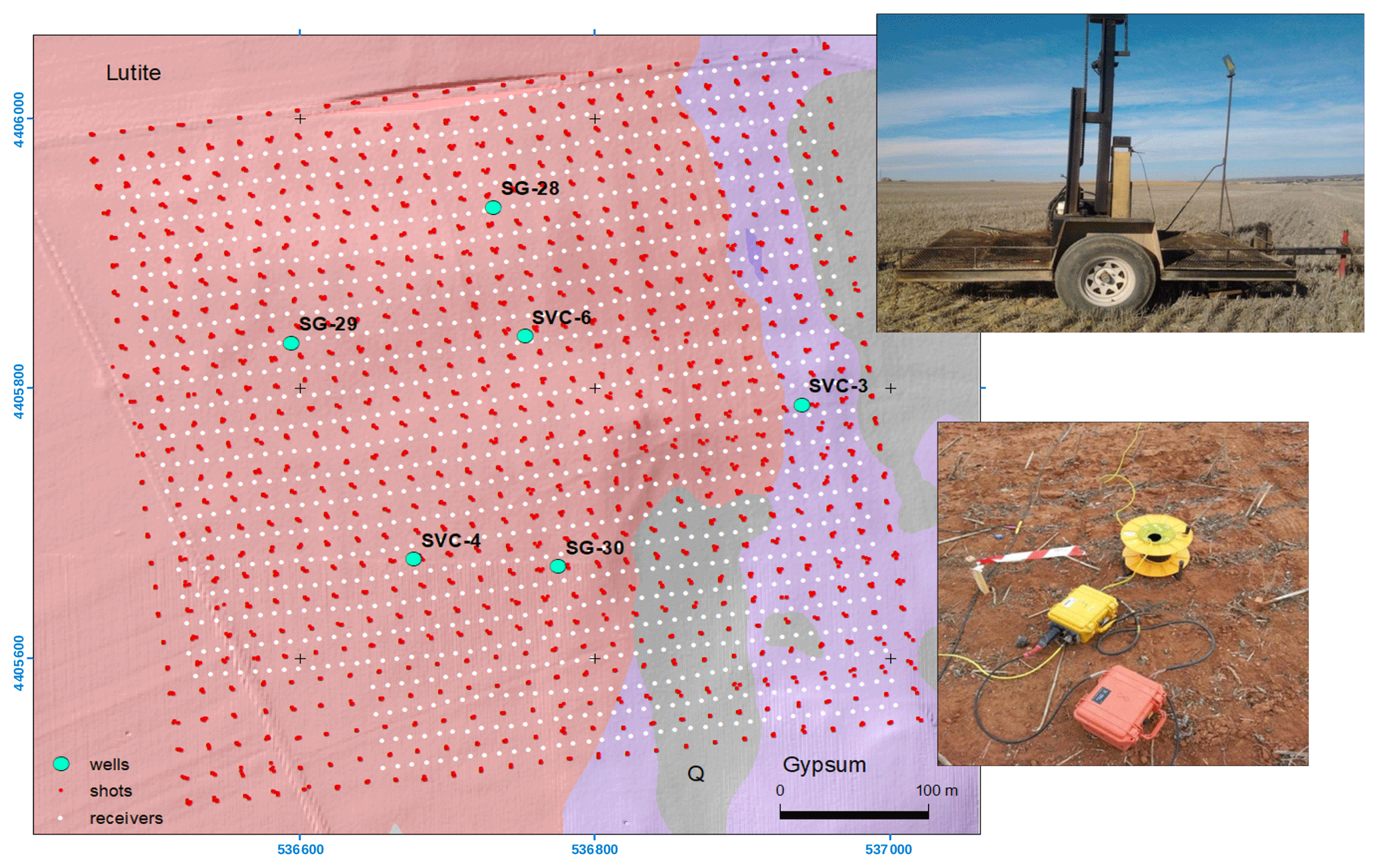
Figure 2Geometry of the acquisition experiment. Red dots mark the positions of the sources, white dots mark the positions of the receivers. Receivers consisted of single vertical-component exploration geophones connected to an array of 10 GEODE (Geometrics) data acquisition systems. Light blue dots indicate drilled boreholes. A 250 kg weight drop was used (from the Inst. Superior Tecnico Lisbon, Portugal).
In the Villar de Cañas syncline (Fig. 1b), the Cenozoic sedimentary sequences are separated from each other by low-angle unconformities. In particular, the outcropping lower and middle Miocene sediments of the second Neogene unit are surveyed by our study (Fig. 1c). They are described as the Balanzas series, made up from bottom to top by the Balanzas gypsum (Y) and the Balanzas lower lutites (LT). The Y includes several types of gypsum alternating with lutites or shales that have been grouped into three units: (i) macrocrystalline and laminated gypsum (Y1); (ii) gypsum, lutites, and marls (Y2); and (iii) gypsum with shaly, marly levels and gypseous alabaster (Ytr) (Fig. 1). The LT outcrops in the core of the Villar de Cañas syncline and contains red siltstones and mudstones with some gypsum and/or sands (Fig. 1).
According to the second Neogene unit sequence, gypsum rocks are the main lithological target in the study area. The definition of their internal structure and the boundaries between the different sequences are often difficult, considering the heterogeneity of these deposits. Gypsum (CaSO4⋅2H2O) is frequently affected by diagenetic processes and, as a consequence, gypsum rocks include clay, carbonates and other minerals. The presence of other minerals affects the purity of the gypsum rocks and this is reflected in changes of its physical properties potentially measurable with geophysical methods (Carmichael, 1989; Guinea et al., 2010; Festa et al., 2016). However, their variability in composition and their complex geometry make the characterization of these deposits challenging (Martinius et al., 2002; Diaz-Molina and Muñoz-Garcia, 2010; Escavy et al., 2012; Kaufman and Romanov, 2017). In this case, the high-resolution seismic characterization of the site was designed by taking into account all of these structural and lithological constraints.
To provide a detailed image of the target site shallow subsurface, we designed a dense 3-D tomographic survey to ensure a high spatial resolution. The approximately regular acquisition grid covered an area of 500 m×500 m. Source locations were distributed in a grid of 20 m×20 m cells. Receivers were distributed along profiles oriented east–west, with 20 m spacing. Along each line, 48 receivers were distributed with a receiver spacing of 10 m (Fig. 2). The seismic source consisted of a 250 kg accelerated weight drop. The seismic data acquisition system consisted of ten 24-channel GEODE ultra-light seismic recorders (Geometrics systems) that resulted in a 240-channel system. Each channel included a conventional vertical-component geophone. With the available instrumentation, the acquisition scheme required five swaths to cover the entire study area. Each swath consisted of five active receiver lines (240 channels), giving a total of 676 source shot positions resulting in a total of 3380 shot gathers. The survey was acquired and completed in two different time periods (December 2013 and January 2014). The acquisition program was carefully adapted to account for the special circumstances associated with the acquisition of different swaths at different times, and with different environmental conditions (e.g., different levels of ambient noise, weather changes, or potential technical problems in acquisition equipment). One of the main concerns was to ensure the release of enough acoustic energy for all of the available offsets, especially in the presence of complicated weather conditions. The 250 kg accelerated weight drop source ensured high signal-to-noise (S∕N) ratios in most of the shot points (Fig. 3). However, some of them required repetition of the shot to improve the S∕N ratio by means of raw data stacking. Despite the complexity of the seismic acquisition, the recorded seismic data were of high quality and high S∕N ratio and allowed for a well-defined picking of first arrivals (Fig. 3) corresponding to almost all the offset range, reaching maximum offsets of almost 700 m. The high quality of the seismic first arrivals favored the semiautomatic picking of more than half a million of the first breaks.
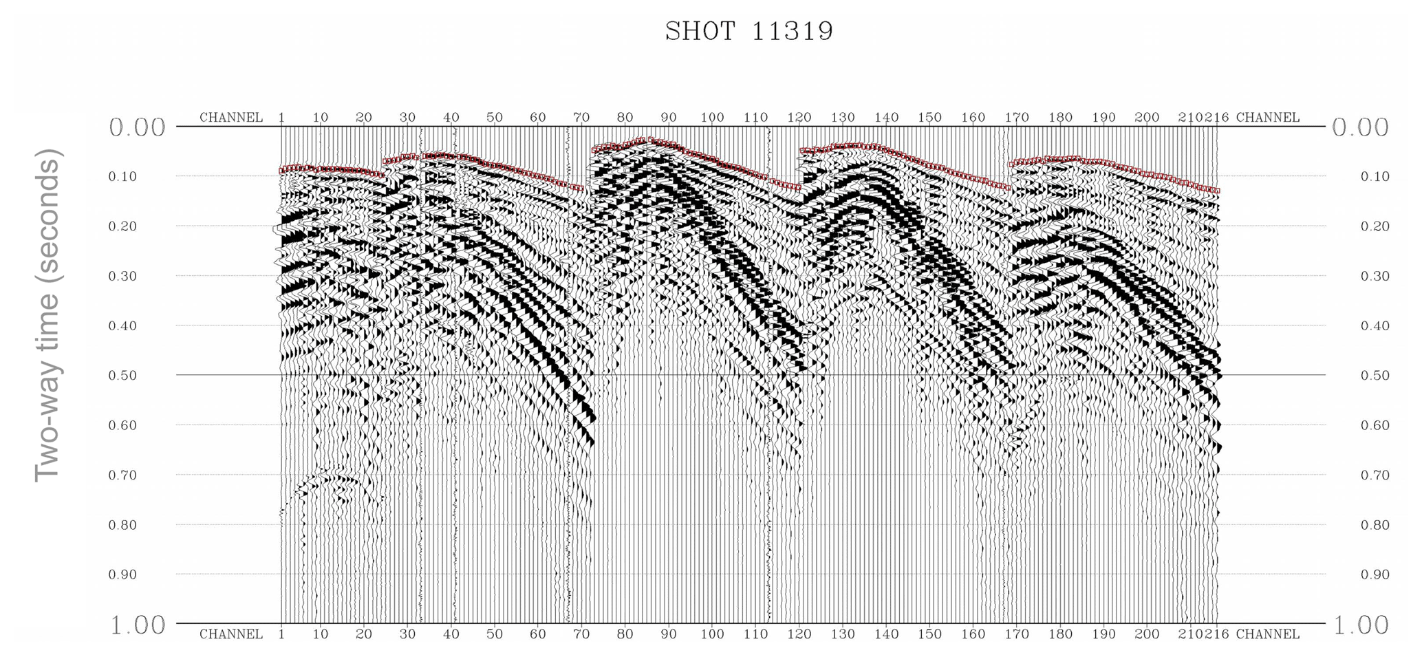
Figure 3Example of shot gather recorded by the array of 10 GEODES seismic recorders (24 channels each). The red symbols indicate the travel-time picks of the firsts arrivals used as inputs for the tomographic inversion. Trace balancing (window times: 0–1500 ms) has been applied to the data for display purposes.
The algorithm used with these data (Pstomo_eq) is a fully 3-D travel time tomographic inversion code (Benz et al., 1996; Tryggvason et al., 2002). The forward modeling is a first-order finite-difference approximation of the eikonal equation, computing all the time field from a source (or receiver) to all of the cells of the model (two different schemes are available based on Hole and Zelt, 1995, and Tryggvason and Bergman, 2006). The travel times to all receiver or source positions are computed from the resulting time field and ray tracing is performed backwards, perpendicular to the isochrons (Vidale, 1988; Hole, 1992). The inversion is performed with the conjugate gradient solver LSQR (Paige and Saunders, 1982). One of the main requirements for a successful inversion is the selection of an appropriate initial model (Kissling, 1988; Kissling et al., 1994). A good approximation to the minimum starting model is the use of the a priori information available for the area, based on the surface geology and the geophysical data previously acquired. In our case, an initial 1-D model was built based on the sonic log information available for different boreholes located within the study area (Fig. 2). The shallow target of the tomographic experiment and the well-controlled sedimentary sequence expected at these depths, with a noncomplex laterally changing geology, favored the election of a very proper initial model.
The particular acquisition pattern carried out in different swaths forced to establish a careful quality control over the data. These factors may introduce some bias to the first arrivals picks (Fig. 3) that could affect the convergence of the inversion algorithm. To avoid any potential error associated with the different conditions during the acquisition we decided to invert all the swaths independently to check the data quality and their convergence. Once convergence was tested in every swath, the other swaths were gradually added into the inversion. This resulted in a relevant improvement in the lateral resolution and a better definition of the final velocity model. The inversion of single swaths was also used to test the dependence of the result on the choice of initial models. Different initial 1-D velocity models based on the previous geophysical and geological information were built to analyze the consistency with the first break picks and the robustness of the inversion. The best fitting 1-D model chosen provided a root mean square (RMS) reduction of 93 % showing a clear 2-D trending geometry in the east–west direction. Taking into account this feature, which was also observed in the surface geology (Figs. 1 and 2) as well as the borehole information, an initial 2-D velocity model was built. This initial model was then used to speed up the convergence of the calculations and to reduce the number of iterations needed to reach the optimal final RMS misfit.
The inversion cell size decreased during the integration of the first arrival picks corresponding to the different swaths. Due to the sparse distribution of receivers in the north–south direction, the cell size corresponding to this direction was the most sensitive to the addition of new travel-time picks to the inversion. Obviously, the reduction of the inversion cell size was also relevant to increase the resolution of the final velocity model, resulting in a final inversion grid spacing of m (for ).
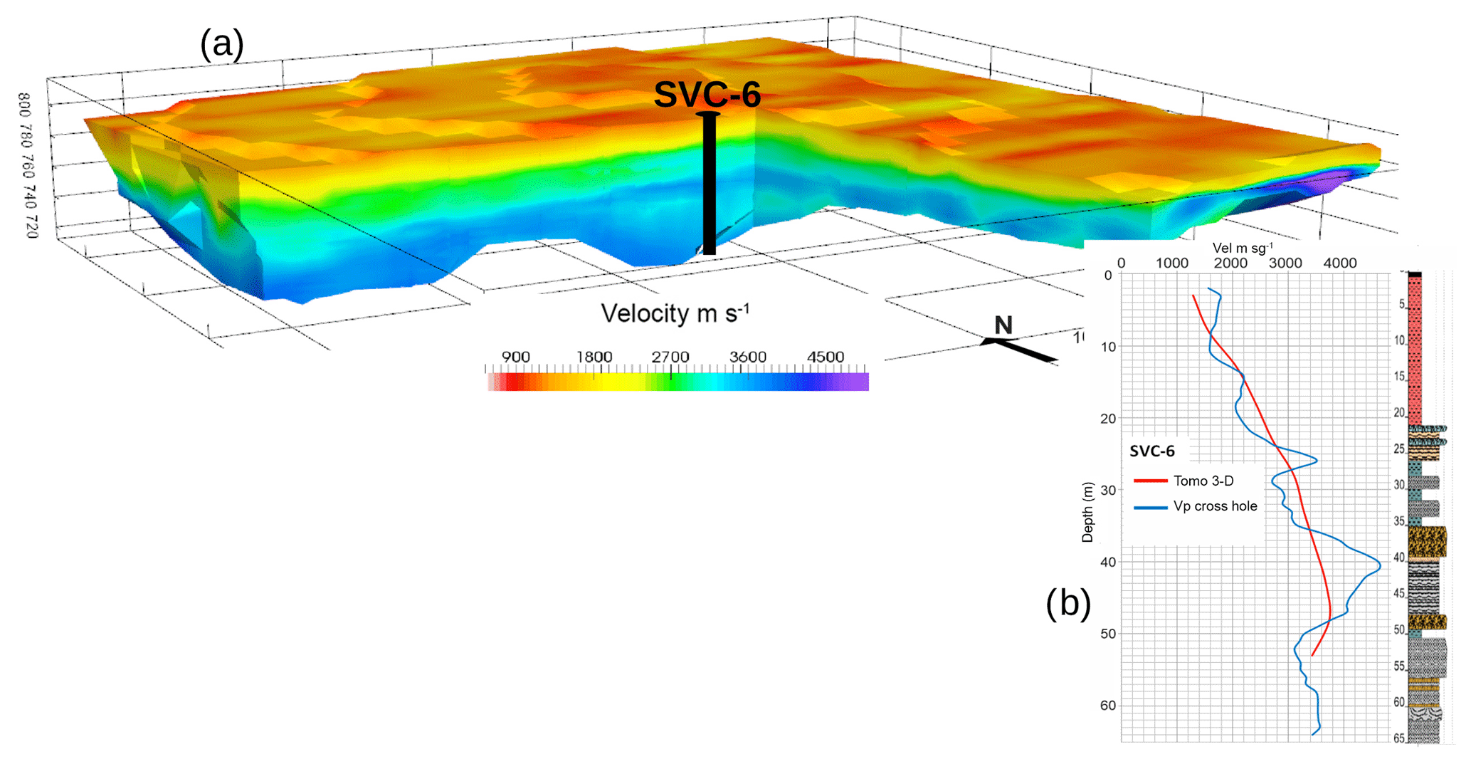
Figure 4(a) 3-D seismic compressional wave velocity model (Vp) derived from the over 500 000 travel-time picks of the first arrivals in the shot gathers. The velocity range goes from nearly 900 m s−1 (reds) to over 4500 m s−1 (blues). (b) Comparison between the smoothly resampled Vp log derived from the sonic data at borehole SVC-6 (light-blue) and the vertical Vp profile extracted from the block at the location of the SVC-6 site indicated by a black arrow in the block. The resampling of the log was carried out so that it would be comparable to the grid size used for the parametrization of the velocity model, which in this case is of m.
The inverted final velocity model shows a detailed image of the shallow subsurface of the study area (Fig. 4). This model provides the best fitting result featuring a final RMS travel time residual of 2.5 ms, which is indicative of the good convergence of the inversion process. According to the ray-path coverage obtained during the inversion, the velocity model retrieves the internal structure of the subsurface with a maximum depth of 120 m (Fig. 4), especially in the central and western sector of the survey. This recovering depth decreases drastically towards the east. This was partly due to the usual ray coverage decrease close to the boundaries of the survey but also to other different causes. The lateral changes in surface geology in this sector affected seismic source coupling, reducing the overall energy injected into the subsurface and affecting the seismic source repeatability. This issue hindered the identification of the first arrivals in a wide range of offsets for the shot points located in the eastern part of the study area (Fig. 4). Furthermore, the high velocity gradient observed at very shallow surface also affects the depth of the traced ray paths.
The direct observation of the 3-D P-wave velocity model reveals several interesting features about the shallow subsurface and its internal structure. The tomographic model shows that the shallowest subsurface (first 5–10 m) is characterized by a very low seismic velocity. This upper layer seems to have a relatively constant depth for the entire study area. Beneath, there is a velocity gradient smoother towards the northwest, slightly increasing to the south and significantly to the east (Fig. 4). This effect is remarkable in the northeast corner of the study area, where the velocity rises from 1000–1200 m s−1 in the shallow surface up to 4000–4500 m s−1 in the first 20–30 m (Fig. 4). This results in a wedge geometry of the velocity model, indicating a clear northwest-dipping trend of the main structural features. Another significant result is the lateral changes in velocity observed in the deepest part of the model, which could suggest the presence of lateral lithological changes.
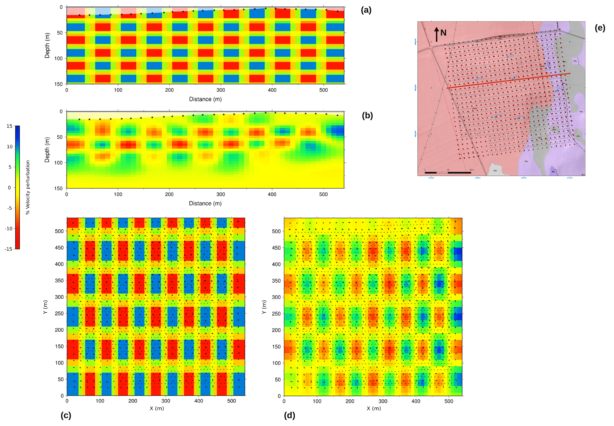
Figure 5Checkerboard tests taking into account the real acquisition geometry on a model involving velocity anomalies of dimensions m and 10 % velocity perturbation. (a) Cross section of the input synthetic velocity model consisting of box anomalies. (b) Cross section across the recovered velocity model. The shot points (black dots) define the topography, with respect to the reference level of the inverted model, below which velocity recovery takes place. (c) Depth slice (map view) across the input model showing the synthetic velocity anomalies. (d) Depth slice across the recovered velocity model at a 45–50 m depth with respect to the reference level of the inverted model. (e) Acquisition geometry showing the location of the vertical sections of (a) and (b).
Different checkerboard tests were carried out to estimate the potential resolution of the final velocity models obtained in the tomographic inversion (Fig. 5). These sensitivity tests provide a qualitative estimation of the spatial and depth resolution and the uncertainty in the experimental design used. The main idea is to test how well the acquisition geometry (distribution of sources and receivers) is able to recover a regular distribution of velocity anomalies. Checkerboard tests only provide indirect evidence of these measures (Lévêque et al., 1993; Rawlinson and Spakman, 2016). These tests illustrate where or what parts of the subsurface models are best resolved. The information that these tests reveal is similar to the resolution and covariance matrix measures obtained by other conventional schemes. For example, covariance matrix methods in LSQR (Yao et al., 1999) give incomplete information, especially when sources and receivers are located at the surface. In this case, the ray paths are strongly dependent upon the velocity gradient, which implies a significant nonlinearity (Bergman et al., 2004, 2006). Keeping that in mind, several tests, using different sizes for the anomalies, were applied to our data. Two different sections (one east–west and one depth slice, representative of the complexity of the study area) have been selected to illustrate the results of the checkerboard analysis (Fig. 5). First of all, an east–west section located at the central part of the tomographic 3-D volume shows that the velocity anomalies are retrieved for the first 100 m in almost all of the study area, slightly reducing its depth of penetration close to the eastern sector. This fact was expected, due to the lower quality of the first arrivals of the shots located in this area. The travel-time picking carried out in this area was very limited in offset, which clearly impeded signals to reach deeper exploration depths. On the other hand, a section at constant depth shows a very homogeneous distribution of the anomalies recovered from the checkerboard test. At 45–50 m depth the resolution analysis assures that the ray coverage is homogeneous and well distributed throughout the entire surface. The least covered area corresponds to the north and the southwestern parts. Although these areas correspond to the boundaries of the study area, where lower resolution is expected, technical problems with the geophone cables forced us to disconnect 24 of the 48 channels in the northernmost receiver line and 12 channels in the southwestern sector in four receiver lines in a row. In spite of these acquisition issues, the checkerboard analysis demonstrates the capability of our experimental system to image the shallow subsurface with sufficient detail.
Despite the velocity model provides a detailed image of the shallow subsurface, a direct geological interpretation is difficult, especially in terms of structural features. Interval velocities from well logs are critical for a realistic interpretation of the 3-D tomographic model so that the internal structure of the shallow subsurface can be geologically inferred.
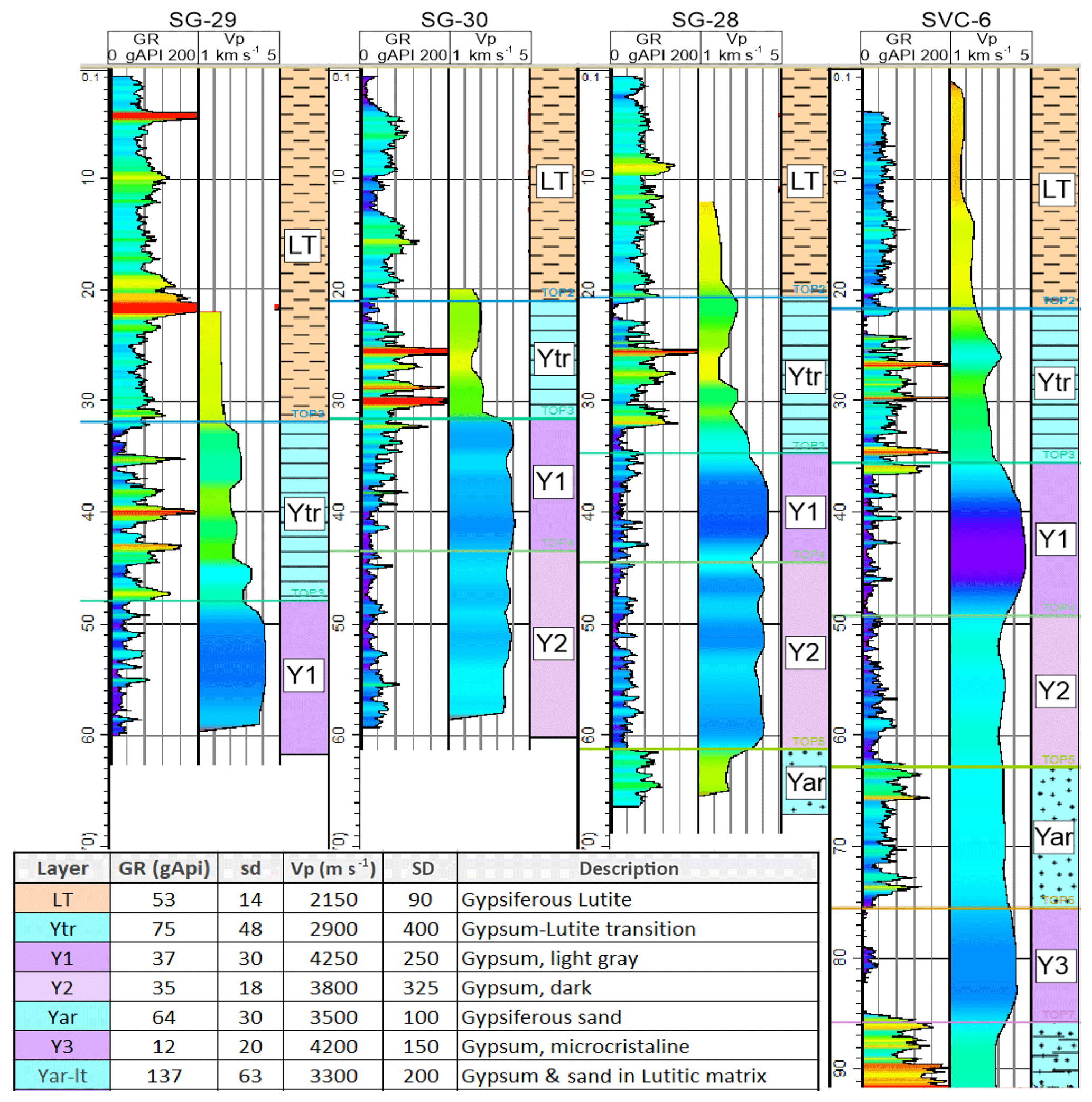
Figure 6Drill holes in the target area with the borehole geophysical logs used in this study. This reveals the correlation between the rock samples, its description and the values of the physical properties (gamma ray, GR; sonic logs, Vp). The top part of the figure reveals the logged data with the correlation between the available boreholes. The bottom table defines the summary criterion used for the interpretation of the different lithologies. The Vp value should be representative of the corresponding lithologies. This criterion is used later in the text to differentiate between the different lithologies in the velocity cube obtained from the tomographic inversion. The left column identifies the location of the boreholes within the acquisition geometry of the seismic survey with the outcropping geology of the target area.
As mentioned above, the study area was covered by an extensive borehole drilling campaign (including geotechnical and geophysical boreholes with core sampling) and a very detailed surface geology mapping, which provided the necessary information to properly decode the geological meaning of the P-wave velocity model. Within the study area, only four geophysically equipped wells were available, and used to guide the interpretation of the velocity model (boreholes: SG-29, SG-30, SG-28 and SVC-6, shown in Fig. 6). The velocity logs, the tailings and the core samples were critical to linking the different lithologies to the geophysical responses. The lithology and the tomographic image were linked by correlating the velocity profiles obtained from the tomographic model with those determined from the sonic logs. This correlation required a homogenization so that the scales of resolution of both methods would be comparable. The 3-D tomographic images are built as velocity grids with cell dimensions of m (). This indicates that the sampling interval in the vertical (z) direction is 5 m, while the sample rate in the z axis of the logs is on the centimeter scale. Thus, the P wave seismic velocity (Vp) logs needed to be resampled to provide average interval velocities in 5 m intervals, representative of the average lithology within this interval. Two resampling approaches were tested. First the log was averaged using a 5 m averaging window, and then resampled in 5 m intervals (Fig. 4); window lengths from 2.5 to 10 m were also tested, but provided similar results. A median filter approach, that avoids extreme values, was also evaluated, providing a similar response, so the 5 m interval average method was finally selected. This homogenization step assured that length-scales of the features observed in both data sets were comparable.
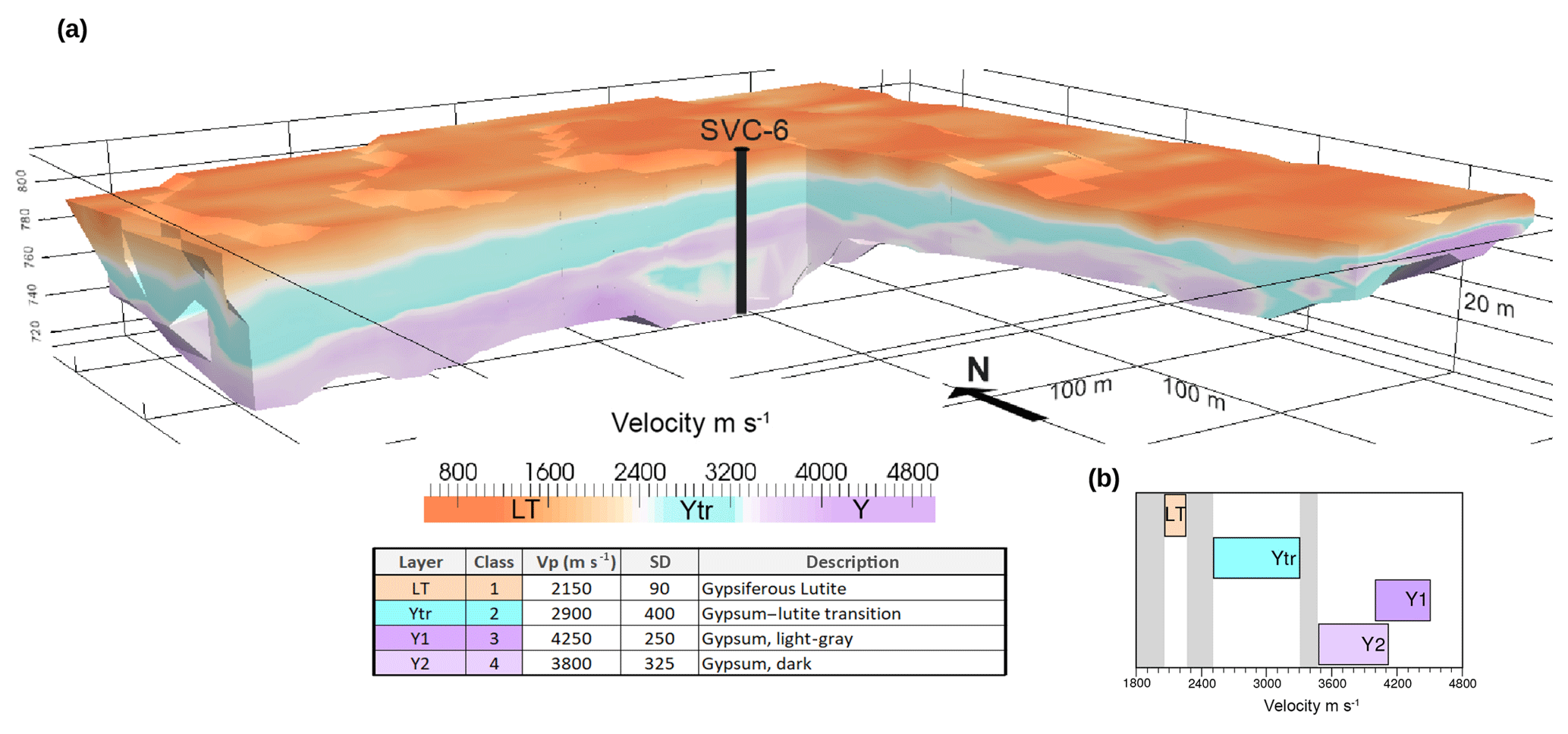
Figure 7(a) 3-D seismic velocity model grid of the shallow subsurface color coded according to the interpreted lithologies derived from Fig. 6. Four different units have been identified: LT, lutites; Ytr, the gypsum–lutite transition layer; and Y1 and Y2, gypsum units. (b) Graph showing the velocity ranges established and the gaps between them. These gaps correspond to seismic velocities that do not have lithologies assigned.
The information derived from the well logs provided constraints to interpret up to nine lithological subunits (Fig. 6). However, the relatively reduced overall depth coverage of the tomographic image means that only four of these units may be identified in the velocity model (Figs. 4 and 6). Characteristic lower and upper limits as well as average seismic propagation velocities for P-waves were estimated for each different lithological unit using the sonic log measurements, resulting in the table scale shown in Fig. 6.
The gamma-ray logs are the most complete logs in the available boreholes, which makes them crucial to define the first lithological boundary at depth (Fig. 6). The velocity data is sparser than the gamma-ray data, and only the borehole SVC-6, located in the central part of the study area (Fig. 2), provides an almost complete velocity log as a result of the combination of the downhole data and the sonic log. The analysis of the well data differentiates a first upper layer that according to the core samples corresponds to the Balanzas lower lutites (LT). This sedimentary rock consists mostly of clay minerals with large openings in their crystal structures, in which K, Th and U fit well. This fact makes the gamma-ray measurements ideal for its identification because they are very sensitive to the presence of natural radioactivity. A sudden decrease in the gamma-ray values clearly defines the transition to a new lithology (Fig. 6). The direct observation of the SVC-6 velocity log shows two well-distinguished sections characterized by different seismic velocities. The recorded values are relatively low (<2000 m s−1) for the first 10–12 m, with a sudden increase at this depth up to 2200 m s−1, keeping this velocity relatively constant until the transition zone (∼24 m) (Fig. 6). The boundary with the deeper formations is observed in Vp with a gradual increase in the velocity values close to 3000 m s−1, which takes place in a few meters indicating a smooth transition in terms of velocities. From the log analysis it can also be inferred that the thickness of the LT layer is almost constant in north–south direction in the central part of the study area (around 20 m depth in SG-28, SG-30 and SVC-6), increasing its thickness to 32 m in the western sector in which SG-29 is located. The lack of logged information in the eastern part of the study area forces the interpretation to rely solely on the information from the surface geology (Fig. 2) The geological map shows the presence of this lithological interface located in the eastern sector of the study area, with an approximate orientation north–south being suddenly moved to the west in the middle part of the study area. This interface puts in contact the lutites layer with the next lithology identified in the core samples. This fact suggests that the layers dip gently to the west supporting the wedge geometry observed in the tomographic model and following the regional-scale geologic interpretations (Biete et al., 2012; Piña-Varas et al., 2013).

Figure 8Resulting shallow subsurface structure represented as detailed cross sections. Cross sections integrate the velocity model derived from the tomography, the constraints provided by the boreholes and the extrapolation of surface geology data (in discontinuous drafted lines). Four different east–west and north–south cross sections are shown with their locations within the study area.
Just beneath the LT layer, the core samples show the presence of a gypsum–lutite transition layer of nearly constant thickness in most of the study area (at least according to the logged information available) with a local increase in thickness in the western sector. This unit, called Ytr, belongs to the second Neogene unit and is characterized by mainly gypsum with centimeter- to meter-scale intercalations of shaly, marly levels. These lithological changes are characterized by a high variability in the recorded sonic and gamma-ray log values. The presence of these gypsiferous shales are clearly observed in the gamma-ray logs, featuring high peaks related to the shaly intercalations. In the sonic logs, the velocity seems to increase in the upper part of the unit with a decrease that coincides with a higher presence of the shaly-marly levels (increase in the gamma-ray log): close to the transition to the next lithology, the sonic log seems to recover the velocity values observed in the upper part.
A great increase in the velocity together with a sudden decrease in the gamma-ray values indicates the transition to a thick lithological sequence of gypsum at depth. In terms of borehole logging, several subunits can be inferred according to the different signatures observed. However, only two of these gypsum units, defined in the geological setting, can be observed in the tomographic model taking into account the depth achieved with the acquisition geometry used. The upper unit (Y1) is defined by higher values of seismic velocities (∼4250 m s−1) than the deeper unit (Y2, ∼3800 m s−1).
The identification of the main lithological units by means of the logged data and the core samples provides a solid link between the geology and the physical properties that allow us to lay out a structural interpretation the 3-D tomographic volume. The standard deviation of every averaged velocity value was used to estimate a rough velocity range corresponding to each lithology but also provided a qualitative measurement uncertainty in the assigned velocity to the different lithologies. This criterion was then used to correlate each P-wave velocity value of the mesh to the defined lithologies (Fig. 7). Looking at the velocities table, the LT layer seems to be the most well-established value, according to the standard deviation obtained, which is the lowest (90 m s−1). Nevertheless, this layer was defined by only using the deeper portion of the log data corresponding to this section; this deeper portion probably corresponds to the higher velocities for this formation neglecting the low values that should be expected at shallow depths, which would significantly increase the standard deviation. This is the case of the Ytr layer which features a standard deviation of 400 m s−1 which clearly reflects the high variability in the seismic velocities observed in the sonic logs.
This velocity analysis allowed us to reimage the tomographic models based on the ranges of velocities defined from the well log data. In this way, we could map the defined lithologies in the velocity model defining their respective boundaries. As a result of this interpretation, different velocity ranges had no direct assignment to lithologies, a result of the lack of overlap in the guided interpretation. These observed gaps mainly affect the definition of the limits between units, which introduce a qualitative measure of their ambiguity (Fig. 7).
The direct observation of the guided interpreted tomographic model allow us to provide geological meaning to the main features previously described. The defined upper boundaries present an undulating character that reveals channel-like structures with an east–west orientation. Note that the sedimentary environment during the upper Oligocene to lower Miocene was a meander setup (Diaz-Molina, 1993). Furthermore, the LT and the Ytr layers appear to increase their thickness towards the west keeping it constant in the north–south direction (Figs. 7 and 8), which indicates that the gypsum layers are dipping towards the west. This coincides with the wedge geometry clearly observed in the tomographic velocity models (Fig. 4). The latter was also suggested by the regional-scale geology and other geophysical studies (Biete et al., 2012; Piña-Varas et al., 2013).
In order to validate the accuracy of the log-guided interpretation of the tomographic model, several 2-D velocity sections at depth were extracted following different existing east–west and north–south geological profiles. Those selected profiles correspond to geological cross sections based on data collected at surface and the interpretation of the core samples of the existing single boreholes. Besides, the interpreted boreholes used in this study were projected to the closest profiles, thus providing additional information to compare and evaluate the final structural interpretation of the 3-D velocity grid. In addition to these wells (SG-29, SG-30, SG-28 and SVC-6), two more interpreted wells were projected (SVC-4 and SVC-3) to provide geological interpretation to the uncovered areas. Unfortunately, in these two wells there were no available velocity logs.
The definition of the different lithological boundaries was of great interest in this study. In this sense, the resulting images show a general good agreement between the geological cross sections, the interpreted boreholes and the tomographic models, in terms of boundary definitions, geometry and depth throughout all of the 3-D volume (Fig. 8). The matching between hard data (surface geology plus well log data) and soft data (seismic tomography) is quite consistent taking into account the different criteria used and resolution to define the lithological changes at depth. The correlation between both interpretations is particularly significant in the central part of the study area, where the lithological boundaries defined in the geological cross sections even show changes in dip and undulating geometries also retrieved by the seismic velocity models. In those areas, the comparison between the interpreted boreholes projected to the velocity profiles is also in good agreement (Fig. 8). Nevertheless, several discrepancies are observed in specific areas, especially located in the western and eastern ends, affecting different lithological layers, which need to be addressed in detail to finally validate the tomographic models.
From depth to surface, the first units identified are Y1 and Y2 (Fig. 6). From the previous geological analysis, this gypsum units are characterized by a complex internal structure with no clear defined boundary, continuous lateral changes and the presence of widely disperse massive gypsum bodies. The tomographic model seems to corroborate this by showing a quite complex distribution of these two units in the 3-D velocity volume. Unfortunately, the depth resolution of the tomographic model together with the velocity inversion observed between the Y1 and Y2 (Fig. 4) makes it very difficult to provide a reliable retrieval of the seismic velocities associated with each lithology. This issue is well described in the literature, such as in the one described in Flecha et al. (2004). These aspects together with the smooth character of the seismic tomography lead us to consider these gypsum units as a unique lithology, focusing on the upper boundary definition and avoiding the definition of the complex internal structure. Besides, this objective was beyond the scope of the study; and from an engineering point of view, both lithological units can be considered as one unit in terms of mechanical response.
The upper limit between Y1 + Y2 (Y) and Ytr is relatively well constrained in almost all of the area, especially when compared with the log interpretation. Changes in dip and variable geometries at depth observed in the geological cross sections are also imaged by the guided interpretation of the 3-D velocity model (Fig. 8). The well-contrasted seismic velocities between both lithologies observed in the well logs help with the boundary definition, which does not show too much ambiguity. Nevertheless, the limitations of the seismic tomography mentioned before makes it impossible to reach the seismic velocity ranges expected for the gypsum units according to the log data (Fig. 4). The tomography velocity model clearly suggests the velocity inversion in some of the profiles (i.e., profile c-9i in Fig. 8) at this lithological level showing the complex distribution that can be inferred from the velocity log interpretation.
Quite different is the LT–Ytr boundary definition, which seems to be underestimated in deep locations as we move to the western sector of the survey area (Fig. 8). Several considerations can be taken into account to understand this mismatch observed between different interpretations. First, this lithological boundary is relatively diffuse because of the presence of the gypsiferous lutites as intercalations distributed within the gypsum rock. This fact is the cause of the appearance of peaks of higher velocity in the sonic logs which are responsible for the increase in the average velocity of the Ytr unit. Unfortunately, due to the acquisition geometry, the resolution that characterizes the tomographic model is not able to differentiate between these intercalations (lenticular layers of a centimeter to meter scale) within Ytr, which would have helped to define this boundary in greater detail. As mentioned above, we resampled the velocities from sonic logs to correlate their velocities to the tomography results. As a result, the averaged velocity associated with Ytr is characterized with a high standard deviation (Fig. 6). This increases the uncertainty in Ytr identification in the whole tomographic 3-D volume, which induces some mismatch in the unit identification.
On the other hand, the location of the boreholes used for the guided interpretation of the tomographic model also can account for these observed discrepancies. Most of them (SG-28, SVC-6 and SG-30) are located in the central part of the study area and besides this they are aligned in the north–south direction. Thus, the weight of these three boreholes in the estimation of the velocity intervals in both lithologies involved is significant and introduces a bias for the rest of the tomography-guided interpretation. According to these wells, the lutites have a quite similar thickness, placing the lithological boundary at a relatively shallow depth (around 20 m) compared with the same boundary in the western area, which is located at a deeper level. This implies that the velocity derived from the boreholes for the LT layer is most probably underestimated in relation to the expected velocities for this lithology at this part of the survey. The effects of the soil compaction, due to the layer thickening in this sector, could increase the velocity of the lutites at depth. This fact as well as the incompleteness of logs at shallow depths is responsible for the low standard deviation associated with this lithology, which, together with the high values associated the Ytr unit, seems to be a strong effect in the delimitation of this upper boundary when moving to the west. All these factors introduce a high ambiguity in some areas of the model, which leads to a mismatch between the different interpretations. In general, the east–west velocity sections show a better match between geological and tomographic delineation as we move eastwards. Profile c-5i shows a clear example of the impact of all these mentioned factors. The mismatch between models and the interpreted wells is very high in the western sector decreasing close to well SVC-4 in which a high uncertainty in lithological boundary is observed. On the other hand, the north–south sections also show definitive evidence of this. Profile c-9i presents a general good agreement between both interpretations. Note that this profile is practically aligned with boreholes SG-28, SVC-6 and SG-30. Conversely, section c-8i shows a clear discrepancy since it is located further to the west in relation to the c-9i profile (Fig. 8).
The tomographic velocity model suggests the presence of a shallow weathered layer (warm colors in Fig. 4). This layer is clearly observed on the field, the surface mapping and the core samples recovered in most of the geotechnical boreholes. These observations show that this very shallow layer have two different lithologies that correspond to lutites (LT) at the northern and western sector of the study area and also transition gypsum (Ytr) in the eastern sector (Figs. 2 and 6). This upper weathered layer seems to be characterized by low velocity values though, from a seismic velocity point of view, both lithologies are barely distinguishable. Furthermore, the guided interpretation of the tomographic model is also unable to retrieve this layer basically due to the incompleteness of the sonic logs at shallow depths (only downhole data is available for SVC-6, Fig. 6). This is especially significant for the weathered Ytr unit that has no recorded data to estimate its seismic velocity at shallow surface. For this reason, in the guided interpretation this identified weathered layer has not been considered as a differentiated boundary. However, the surface geology offers a perfect way to define the boundary associated between both lithologies in this upper weathered layer (Fig. 8). Methodologically, it indicates that the direct correlation between velocity and lithology might not be applicable when the influence of other factors is relevant. Weathering affects the physical properties of the lithology such as outcropping, decreasing velocities characteristic of the Ytr to values below 2100 m s−1, the upper limit criteria used to identify the LT.
The imaging of the LT–Ytr transition cannot be accomplished by only using the tomographic velocity model, according to the borehole logged data available. More borehole logged data in representative locations of the velocity model are needed to better constrain the velocity range assigned to each lithology, which in turn would enable us to improve the velocity ranges and reduce the standard deviations for each unit. A complete sequence for the sonic logs, from surface to the maximum depth, will be very useful to further constrain the weathered layer and maybe it could offer a clue to differentiate surface lutites from gypsum, from a seismic velocity point of view. Nevertheless, seismic velocity alone seems to have some limitations to clearly define both lithologies or at least there is no clear and unique signature for these two lithologies. For this reason, we believe that adding other physical properties (e.g., resistivity or porosity) could improve the definition of the LT–Ytr transition.
One of the main concerns is the presence of dissolution cavities within the evaporitic sequence, especially taking into account the possible host of a singular infrastructure. In this sense, travel-time tomography is very limited for recovering the location, geometry and velocity values expected for a cavity. Besides, this is particularly more difficult if only surface seismic data are used in the inversion (Flecha et al., 2004). In case of the presence of a cavity, the wavefronts do not propagate through it and the first arrivals are only capable of recording the perturbation due to the large velocity contrast at the edge of the velocity anomaly. Fortunately, the density ray diagrams were revealed as an appropriate tool to define the presence of cavities, which are characterized by a very low or a lack of ray coverage. Taking this into account, the analysis of the ray coverage diagrams derived from the travel-time inversion do not show any evidence of this fact, which implies that no cavities are characterized, at least at the decameter scale (Figs. 4, 5 and 7). Furthermore, the extensive borehole campaign carried out on site also showed no evidence of the presence of cavities in the shallow subsurface.
On the other hand, the presence of potentially active faults in the area is also a main issue in hazard analysis and risk assessment. For this reason, the study of the presence of any nonmapped minor fault and the characterization in depth of mapped ones was also of interest. The study of instrumental and historical seismicity showed that the area was tectonically stable with a very reduced amount of seismic events in the area and of very low magnitude. Furthermore the paleoseismic studies by means of trenches revealed that there is no evidence of recent seismic activity related to any fault system. In the same way, the analysis of the tomographic velocity model supports these statements about evidence of recent faulting responsible for any seismic activity that it could constitute any risk. The lithological units imaged by the velocity models do not show any evidence of faulting, which indicates that this sedimentary package has not been affected by any recent activity (Figs. 7 and 8). This fact supports the evidence shown by other studies carried out in the area.
The detailed 3-D structure of an evaporite sequence in the Villar de Cañas syncline (Cuenca) has been revealed by using high-resolution shallow seismic tomographic inversion of first arrival travel times. The local tomographic image of the evaporite sedimentary sequence allows for observing undulating structures in the base of the boundary layers. The tomographic Vp velocity model interpreted with the aid of additional geological and geophysical observations, such as Vp measurements from sonic logs and core description from boreholes, provided a detailed mapping of the different lithologies that build up the sedimentary evaporite sequence. Additional constraints coming from sonic and gamma-ray logs were proven to be critical in the interpretation of the inverted velocity model, allowing identification of the detailed features and geological structures at depth. Well logs and surface geology data allowed for interpreting the different lithologies in the seismic image. The constraints used consisted on average Vp values and Vp ranges for the different lithologies identified from the description of the core samples extracted from the boreholes. This provided the basis for a pseudo-automatic (geophysically driven) interpretation, where model cells were assigned to a specific lithology according to the Vp value of the corresponding node of the mesh. Despite the relatively complex structure and composition of the target area, the guided interpretation scheme presented in this study results in a very powerful procedure to extract structural information from velocity models. However, the consistency between the model and interpretation reduces its effectiveness when trying to resolve areas characterized by a high uncertainty in the guided interpretation. This is particularly true for the uppermost layers where discrepancies can be accounted for by different factors including the irregular distribution of the boreholes and logged information; overlapping Vp values for different lithologies or composition; and the influence of physical conditions (pressure, temperature, water content). Therefore, in those areas the direct mapping or correlation between velocity and lithology might not be applicable without the help of other constraints, e.g., other geophysical parameters that can provide additional information to distinguish specific lithologies.
The data can be accessed, upon request, from the database server from the Institute of Earth Sciences “Jaume Almera”, ICTJA, CSIC (http://geodb.ictja.csic.es/\#dades1, Institute of Earth Sciences “Jaume Almera”, 2019).
RC, DM and IM conceived and designed the seismic experiment. All the authors had an active participation in data acquisition and processing but also in the discussion, preparation and correction of the manuscript.
The authors declare that they have no conflict of interest.
This work has been supported by projects (ref: CGL2014-56548-P, CGL2016-81964-REDE)
supported by the Spanish Ministry of Science and Innovation, 2017 SGR 1022 Generalitat de
Catalunya, and by ENRESA. The seismic data recording system that consisted of 10 GEODE
seismic recorders (Geometrics) was provided by the GIPP-GFZ Potsdam (Germany). The acoustic energy used as
source was generated by a 250 kg accelerated weight drop provided by the
Instituto Superior Tecnico, University Lisbon, (Portugal) and a 90 kg
accelerated weight drop provided by the University of Oviedo (Spain). The
data are located on the database server from the Institute of Earth Sciences
Jaume Almera, ICTJA, CSIC (http://geodb.ictja.csic.es/\#dades1). We are
very thankful to Christan Haberland, Juan Manuel González Cortina and
Francisco Javier Álvarez Pulgar for their interest in the experiment and
assistance during the field operations. We would also like to thank the
valuable comments of Juan Alcalde that significantly improved the final
manuscript.
Edited by: Michal
Malinowski
Reviewed by: Mariusz Majdanski and Priyank Jaiswal
Alcalde, J., Martí, D., Juhlin, C., Malehmir, A., Sopher, D., Saura, E., Marzán, I., Ayarza, P., Calahorrano, A., Pérez-Estaún, A., and Carbonell, R.: 3-D reflection seismic imaging of the Hontomín structure in the Basque-Cantabrian Basin (Spain), Solid Earth, 4, 481–496, https://doi.org/10.5194/se-4-481-2013, 2013a.
Alcalde, J., Martí, D., Calahorrano, A., Marzan, I., Ayarza, P., Carbonell, R., Juhlin, C., and Pérez-Estaún, A.: Active seismic characterization experiments of the Hontomín research facility for geological storage of CO2, Spain, Int. J. Greenh. Gas Con., 19, 785–795, https://doi.org/10.1016/j.ijggc.2013.01.039, 2013b.
Alcalde, J., Marzán, I., Saura, E., Martí, D., Ayarza, P., Juhlin, C., Pérez-Estaún, A., and Carbonell, R.: 3-D geological characterization of the Hontomin CO2 storage site, Spain: multidisciplinary approach from seismics, well-logging and regional data, Tectonophysics, 627, 6–25, https://doi.org/10.1016/j.tecto.2014.04.025, 2014.
Alonso-Zarza, A. M., Calvo, J. P., Silva, P. G., and Torres, T.: Cuenca del Tajo, in: Geología de España, edited by: Vera, J. A., SGE-IGME, Madrid, 556–561, 2004.
Andara, E., Guillot, E., Carbonell, R., and García-Lobon, J. L: Constraining reflectivity in crystalline environment by using multicomponent VSP data, 73rd European Association of Geoscientists and Engineers Conference and Exhibition: Unconventional Resources and the Role of Technology, Incorporating SPE EUROPEC, 4174–4178, 2011.
Andrés, J., Alcalde, J., Ayarza, P., Saura, E., Marzán, I., Martí, D., Martínez Catalán, J. R., Carbonell, R., Pérez-Estaún, A., García-Lobón, J. L., and Rubio, F. M.: Basement structure of the Hontomín CO2 storage site (Spain) determined by integration of microgravity and 3-D seismic data, Solid Earth, 7, 827–841, https://doi.org/10.5194/se-7-827-2016, 2016.
Baumann-Wilke, M., Bauer, K., Schovsbo, N. H., and Stiller, M.: P-wave traveltime tomography for a seismic characterization of black shales at shallow depth on Bornholm, Denmark, Geophysics, 77, EN53–EN60, https://doi.org/10.1190/geo2011-0326.1, 2012.
Benz, H., Chouet, B. Dawson, P., Lahr, J., Page, R., and Hole, J.: Three dimensional P-and S-wave velocity structure of Redoubt Volcano, Alaska, J. Geophys. Res., 101, 8111–8128, https://doi.org/10.1029/95JB03046, 1996.
Bergman, B., Tryggvason, A., and Juhlin, C.: High resolution seismic traveltime tomography incorporating static corrections applied to a till covered bedrock environment, Geophysics, 69, 1082–1090, https://doi.org/10.1190/1.1778250, 2004.
Bergman, B., Tryggvason, A., and Juhlin, C.: Seismic tomography studies of cover thickness and near-surface bedrock velocities, Geophysics, 71, U77–U84, https://doi.org/10.1190/1.2345191, 2006.
Bernal, I., Tavera, H., Sulla, W., Arredondo, L., and Oyola, J.: Geomorphology Characterization of Ica Basin and Its Influence on the Dynamic Response of Soils for Urban Seismic Hazards in Ica, Peru, International Journal of Geophysics, 2018, 9434251, https://doi.org/10.1155/2018/9434251, 2018.
Biete, C., Roca, E., and Hernáiz-Huerta, P. P.: The Alpine structure of the basement beneath the southern Loranca Basin and its influence in the thin-skinned contractional deformation of the overlying Mesozoic and Cenozoic cover, Geo-Temas, 13, 173–176, 2012.
Bryś, K., Bryś, T., Ara-Sayegh, M., and Ojrzyńska, H.: Subsurface shallow depth soil layers thermal potential for ground heat pumps in Poland, Energ. Buildings, 165, 64–75, https://doi.org/10.1016/j.enbuild.2018.01.015, 2018.
Carbonell, R., Pérez-Estaún, A., Maitínez-Landa, L., Martí, D., and Carretero, G.: Geophysical and geological characterization of fractures within a granitic pluton, Near Surf. Geophys., 8, 181–193, https://doi.org/10.3997/1873-0604.2010002, 2010.
Carmichael, R. S.: Practical handbook of physical properties of rocks and minerals, CRC Press, Inc., 1989.
Davis, T. L., Terrell, M. J., Benson, R. D., Cardona, R., Kendall, R. R., and Winarsky, R.: Multicomponent seismic characterization and monitoring of the CO2 flood at Weyburn Field, Saskatchewan, The Leading Edge, 22, 696–697, https://doi.org/10.1190/1.1599699, 2003.
De Vicente, G. and Muñoz-Martín, A.: The Madrid Basin and the Central system: A tectonostratigraphic analysis from 2D seismic lines, Tectonophysics, 602, 259–285, https://doi.org/10.1016/j.tecto.2012.04.003, 2013.
Diaz-Molina, M.: Geometry and lateral accretion patterns in meander loops: examples from the Upper Oligocene-Lower Miocene, Loranca Basin, Spain, in: International Association of Sedimentologists, Special Publication 17, edited by: Marzo, M. and Puigdefabregas, P., Alluvial Sedimentation, 115–131, 1993.
Diaz-Molina, M. and Muñoz-Garcia, M. B.: Sedimentary facies and three-dimensional reconstructions of upper Oligocene meander belts from the Loranca Basin, Spain, AAPG Bulletin, 94, 241–257, https://doi.org/10.1306/07210909010, 2010.
Díaz-Molina, M. and Tortosa, A.: Fluvial fans of the Loranca Basin, Late-Oligocene-Early Miocene, central Spain, in: Tertiary Basins of Spain, edited by: Friend, P. and Dabrio, C., Cambridge University Press, 300–307, 1996.
Escavy, J. I., Herrero, M. J., and Arribas, M. E.: Gypsum resources of Spain: Temporal and spatial distribution, Ore Geol. Rev., 49, 72–84, https://doi.org/10.1016/j.oregeorev.2012.09.001, 2012.
Escuder Viruete, J., Carbonell, R., Martí, D., Jurado, M. J., and Pérez-Estaún, A.: Architecture of fault zones determined from outcrop, cores, 3-D seismic tomography and geostatistical modeling: Example from the Albalá Granitic Pluton, SW Iberian Variscan Massif, Tectonophysics, 361, 97–120, https://doi.org/10.1016/S0040-1951(02)00586-3, 2003.
Escuder Viruete, J., Carbonell, R., Pérez-Soba, C., Martí, D., and Pérez-Estaún, A.: Geological, geophysical and geochemical structure of a fault zone developed in granitic rocks: Implications for fault zone modeling in 3-D, Int. J. Earth Sci., 93, 172–188, https://doi.org/10.1007/s00531-003-0378-z, 2004.
Festa, V., Tripaldi, S., Siniscalchi, A., Acquafredda, P., Fiore, A., Mele, D., and Romano, G.: Geoelectrical resistivity variations and lithological composition in coastal gypsum rocks: A case study from the Lesina Marina area (Apulia, southern Italy), Eng. Geol., 202, 163–175, https://doi.org/10.1016/j.enggeo.2015.12.026, 2016.
Flecha, I., Martí, D., Carbonell, R., Escuder-Viruete, J., and Pérez-Estaún A.: Imaging low-velocity anomalies with the aid of seismic tomography, Tectonophysics, 388, 225–238, https://doi.org/10.1016/j.tecto.2004.04.031, 2004.
Flecha, I., Carbonell, R., Zeyen, H., Martí, D., Palomeras, I., Simancas, F., and Pérez-Estaún, A.: Imaging granitic plutons along the IBERSEIS profile, Tectonophysics, 420, 37–47, https://doi.org/10.1016/j.tecto.2006.01.019, 2006.
Giese, R., Henninges, J., Lüth, S., Morozova, D., Schmidt-Hattenberger, C., Würdemann, H., Zimmer, M., Cosma, C., Juhlin, C., and CO2SINK Group: Monitoring at the CO2SINK Site: A Concept Integrating Geophysics, Geochemistry and Microbiology, Energy Proced., 1, 2251–2259, https://doi.org/10.1016/j.egypro.2009.01.293, 2009.
Guimerà, J., De Vicente, G., and Rodríguez-Pascua, M. A.: La Rama Castellano-valenciana, in: Geología de España, edited by: Vera, J. A., Sociedad Geológica Española e Instituto Geológico y Minero de España, 610–612, 2004.
Guimerà, J., Rivero, L., Salas, R., and Casas, A.: Moho depth inferred from gravity and topography in an intraplate area (Iberian Chain), Tectonophysics, 666, 134–143, https://doi.org/10.1016/j.tecto.2015.10.021, 2016.
Guinea, A., Playà, E., Rivero, L., Himi, M., and Bosch, R.: Geoelectrical classification of gypsum rocks, Surveys Geophysics, 31, 557–580, https://doi.org/10.1007/s10712-010-9107-x, 2010.
Heincke, B., Günther, T., Dalsegg, E., Rønning, J. S., Ganerød, G. V., and Elvebakk, H.: Combined three-dimensional electric and seismic tomography study on the Åknes rockslide in western Norway, J. Appl. Geophys., 70, 292–306, https://doi.org/10.1016/j.jappgeo.2009.12.004, 2010.
Hole, J. A.: Non-linear high-resolution three-dimensional seismic traveltime tomography, J. Geophys. Res., 97, 6553–6562, https://doi.org/10.1029/92JB00235, 1992.
Hole, J. A. and Zelt, C.: 3-D finite differences reflection traveltimes, Geophysics, 121, 427–434, https://doi.org/10.1111/j.1365-246X.1995.tb05723.x, 1995.
IAEA: Storage of Radioactive Waste Safety Guide IAEA Safety Standards Series No. WS-G-6.1 0608-Waste repositories STI/PUB/1254, ISBN: 92-0-106706-2, 55 pp., 2006.
Institute of Earth Sciences “Jaume Almera”: http://geodb.ictja.csic.es/#dades1, last access: 21 January 2019.
Juhlin, C., Giese, R., Zinck-Jorgensen, K., Cosma, C., Kazemeini, H., Juhojuntti, N., Luth, S., Norden, B., and Förster, A.: 3-D baseline seismics at Ketzin, Germany: the CO2SINK project, Geophysics, 72, B121–B132, https://doi.org/10.1190/1.2754667, 2007.
Kaufmann, G. and Romanov, D.: Geophysical observations and structural models of two shallow caves in gypsum/anhydrite-bearing rocks in Germany Geological Society, London, Special Publications, 466, 6, https://doi.org/10.1144/SP466.13, 2017.
Kazemeini, H., Juhlin, C., and Fomel, S.: Monitoring CO2 response on surface seismic data; a rock physics and seismic modeling feasibility study at the CO2 sequestration site, Ketzin Germany, J. Appl. Geophys., 71, 109–124, https://doi.org/10.1016/j.jappgeo.2010.05.004, 2010.
Kim, J. S., Kwon, S. K., Sanchez, M., and Cho, G. C.: Geological Storage of High Level Nuclear Waste, KSCE Journal Civil Engineering, 15, 721, https://doi.org/10.1007/s12205-011-0012-8, 2011.
Kissling, E.: Geotomography with local earthquakes, Rev. Geophys., 26, 659–698, https://doi.org/10.1029/RG026i004p00659, 1988.
Kissling, E., Ellsworth, W. L., Eberhart-Phillips, D., and Kradolfer, U.: Initial reference models in local earthquake tomography, J. Geophys. Res., 99, 19635–19646, https://doi.org/10.1029/93JB03138, 1994.
Letort, J., Roux, P., Vandemeulebrouck, J., Coutant, O., Cros, E., Wathelet, M., Cardellini, C., and Avino, R.: High-resolution shallow seismic tomography of a hydrothermal area: application to the Solfatara, Pozzuoli, Geophys. J. Int., 189, 1725–1733, https://doi.org/10.1111/j.1365-246X.2012.05451.x, 2012.
Lévêque, J. J, Rivera, L., and Wittlinger, G.: On the use of the checker-board test to assess the resolution of tomographic inversions, Geophys. J. Int., 115, 313–318, https://doi.org/10.1111/j.1365-246X.1993.tb05605.x, 1993.
Malehmir, A., Schmelzbach, C., Bongajum, E., Bellefleur, G., Juhlin, C., and Tryggvason, A.: 3-D constraints on a possible deep >2.5 km massive sulphide mineralization from 2D crooked-line seismic reflection data in the Kristineberg mining area, northern Sweden, Tectonophysics, 479, 223–240, https://doi.org/10.1016/j.tecto.2009.08.013, 2009.
Malehmir, A., Dahlin, P., Lundberg, E., Juhlin, C., Sjöström, H., and Högdahl, K.: Reflection seismic investigations in the Dannemora area, central Sweden: Insights into the geometry of polyphase deformation zones and magnetite-skarn deposits, J. Geophys. Res., 116, B11307, https://doi.org/10.1029/2011JB008643, 2011.
Malehmir, M., Tryggvason, A., Lickorish, H., and Weihed, P.: Regional structural profiles in the western part of the Palaeoproterozoic Skellefte Ore District, northern Sweden, Precambrian Res., 159, 1–18, https://doi.org/10.1016/j.precamres.2007.04.011, 2007.
Martí, D., Carbonell, R. R., Tryggvason, A., Escuder, J., and Pérez-Estaún, A.: Calibrating 3-D tomograms of a granitic pluton, Geophys. Res. Lett., 29, 15-1–15-4, https://doi.org/10.1029/2001GL012942, 2002a.
Martí, D., Carbonell, R., Tryggvason, A., Escuder, J., and Pérez-Estaún A.: Mapping brittle fracture zones in three dimensions: High resolution traveltime seismic tomography in a granitic pluton, Geophys. J. Int., 149, 95–105, https://doi.org/10.1046/j.1365-246X.2002.01615.x, 2002b.
Martí, D., Carbonell, R., Escuder-Viruete, J., and Pérez-Estaún, A.: Characterization of a fractured granitic pluton: P- and Swaves' seismic tomography and uncertainty analysis, Tectonophysics, 422, 99–114, https://doi.org/10.1016/j.tecto.2006.05.012, 2006.
Martí, D., Carbonell, R., Flecha, I., Palomeras, I., Font-Capó, J., Vázquez-Suñé, E., and Pérez-Estaún, A.: High-resolution seismic characterization in an urban area: Subway tunnel construction in Barcelona, Spain Geophysics, 73, B41–B50, https://doi.org/10.1190/1.2832626, 2008.
Martinius, A. W., Geel, C. R., and Arribas, J.: Lithofacies characterization of fluvial sandstones from outcrop gamma-ray logs (Loranca Basin, Spain): the influence of provenance, Petrol. Geosci., 8, 51–62, https://doi.org/10.1144/petgeo.8.1.51, 2002.
Muñoz-Martin, A. and De Vicente, G.: Cuantificación del acortamiento alpino y estructura en profundidad del extremo sur-occidental de la Cordillera Ibérica (Sierras de Altomira y Bascuñana), Revista Sociedad Geológica de España, 11, 233–252, 1998.
Novitsky, C. G., Holbrook, W. S., Carr, B. J., Pasquet, S., Okaya, D., and Flinchum, B. A.: Mapping Inherited Fractures in the Critical Zone using Seismic Anisotropy from Circular Surveys, Geophys. Res. Lett., 45, 3126–3135, https://doi.org/10.1002/2017GL075976, 2018.
Ogaya, X., Alcalde, J., Marzán, I., Ledo, J., Queralt, P., Marcuello, A., Martí, D., Saura, E., Carbonell, R., and Benjumea, B.: Joint interpretation of magnetotelluric, seismic, and well-log data in Hontomín (Spain), Solid Earth, 7, 943–958, https://doi.org/10.5194/se-7-943-2016, 2016.
Paige, C. C. and Saunders, A.: LSQR: An algorithm for sparse linear equations and sparse least squares, ACM Transactions on Mathematics Software, 8, 43–71, https://doi.org/10.1145/355984.355989, 1982.
Piña-Varas, P., Ledo, J., Queralt, P., Roca, E., García-Lobón, J.L., Ibarra, P., and Biete, C.: Two-dimensional magnetotelluric characterization of the El Hito Anticline (Loranca Basin, Spain), J. Appl. Geophys., 95, 121–134, https://doi.org/10.1016/j.jappgeo.2013.06.002, 2013.
Place, J., Malehmir, A., Högdahl, K., Juhlin, C., and Persson Nilson, K: Seismic characterization of the Grängesberg iron deposit and its mining-induced structures, central Sweden, Interpretation, 3, SY41–SY56, https://doi.org/10.1190/INT-2014-0212.1, 2015.
Rawlinson, N. and Spakman, W.: On the use of sensitivity test in seismic tomography, Geophys. J. Int., 205, 1221–1243, https://doi.org/10.1093/gji/ggw084, 2016.
Samyn, K., Travelletti, J., Bitri, A., Grandjean, G., and Malet, J. P.: Characterization of a landslide geometry using 3-D seismic refraction traveltime tomography, J. Appl. Geophys., 86, 120–132, https://doi.org/10.1016/j.jappgeo.2012.07.014, 2012.
Seillé, H., Salas, R., Pous, J., Guimerà, J., Gallart, J., Torne, M., Romero-Ruiz, I., Diaz, J., Ruiz, M., Carbonell, R., and Mas, R.: Crustal structure of an intraplate thrust belt: The Iberian Chain revealed by wide-angle seismic, magnetotelluric soundings and gravity data, Tectonophysics, 663, 339–353, https://doi.org/10.1016/j.tecto.2015.08.027, 2015.
Sopeña, A. and De Vicente, G.: Cordilleras Ibérica y Costero-Catalana, 5.1. Rasgos generales, in: Geología de España, edited by: Vera, J. A., SGE-IGME, Madrid, 467–470, 2004.
Steeples, D. W.: Engineering and environmental geophysics at the millenium, Geophysics, 66, 31–35, https://doi.org/10.1190/1.1444910, 2001.
Tryggvason, A. and Bergman, B.: A traveltime reciprocity discrepancy in he Podvin and Lecomte time3d finite difference algorithm, Geophys. J. Int., 165, 432–435, https://doi.org/10.1111/j.1365-246X.2006.02925.x, 2006.
Tryggvason, A., Rognvaldsson, S. T., and Flovenz, O. G.: Three-dimensional imaging of the P- and S-wave velocity structure and earthquake locations beneath Southwest Iceland, Geophys. J. Int., 151, 848–866, https://doi.org/10.1046/j.1365-246X.2002.01812.x, 2002.
Ugalde, A., Villaseñor, A., Gaite, B., Casquero, S., Martí, D., Calahorrano, A., Marzán, I., Carbonell, R., and Pérez-Estaún, A.: Passive seismic monitoring of an experimental CO2 geological storage site in Hontomín (Northern Spain), Seismol. Res. Lett., 84, 75–84, https://doi.org/10.1785/0220110137, 2013.
Vegas, R., Vazquez, J. T., Suriñach, E., and Marcos, A.: Model of distributed deformation, block rotations and crustal thickening for the formation of the Spanish Central System, Tectonophysics, 184, 367–378, https://doi.org/10.1016/0040-1951(90)90449-I, 1990.
Vidale, J.: Finite-difference calculation of traveltimes, B. Seismol. Soc. of Am., 78, 2062–2076, 1988.
Wadas, S. H., Tanner, D. C., Polom, U., and Krawczyk, C. M.: Structural analysis of S-wave seismics around an urban sinkhole: evidence of enhanced dissolution in a strike-slip fault zone, Nat. Hazards Earth Syst. Sci., 17, 2335–2350, https://doi.org/10.5194/nhess-17-2335-2017, 2017.
Witherspoon, P. A. Cook, N. G., and Gale, J. E.: Gale Geologic storage of radioactive waste: field studies in Sweden, Science, 211, 4485, 894–900, https://doi.org/10.1126/science.7466363, 1981.
Yao, Z. S., Roberts, R. G., and Tryggvason, A.: Calculating resolution and covariance matrices for seismic tomography with the LSQR method, Geophys. J. Int., 138, 886–894, https://doi.org/10.1046/j.1365-246x.1999.00925.x, 1999.
Yordkayhun, S., Juhlin, C., Giese, R., and Cosma, C.: Shallow velocity-depth model using first arrival traveltime inversion at the CO2SINK site, Ketzin, Germany, J. Appl. Geophys., 63, 68–79, https://doi.org/10.1016/j.jappgeo.2007.05.001, 2007.
Yordkayhun, S., Juhlin, C., and Norden, B.: 3-D seismic reflection surveying at the CO2SINK project site, Ketzin, Germany: A study for extracting shallow subsurface information, Near Surf. Geophys., 7, 75–91, https://doi.org/10.3997/1873-0604.2008036, 2009a.
Yordkayhun, S., Tryggvason, A., Norden, B., Juhlin, C., and Bergmann, B.: 3-D seismic traveltime tomography imaging of the shallow subsurface at the CO2SINK project site, Ketzin, Germany, Geophysics, 74, G1–G15, https://doi.org/10.1190/1.3026553, 2009b.
Zelt, C., Azaria, A., and Levander, A: 3-D seismic refraction traveltime tomography at a groundwater contamination site, Geophysics, 71, H67–H78, https://doi.org/10.1190/1.2258094, 2006.