Full-waveform inversion of short-offset, band-limited seismic data in the Alboran Basin (SE Iberia)

We present a high-resolution P-wave velocity model of the sedimentary cover and the uppermost basement to ∼3 km depth obtained by full-waveform inversion of multichannel seismic data acquired with a 6 km long streamer in the Alboran Sea (SE Iberia). The inherent non-linearity of the method, especially for short-offset, band-limited seismic data as this one, is circumvented by applying a data processing or modelling sequence consisting of three steps: (1) data re-datuming by back-propagation of the recorded seismograms to the seafloor; (2) joint refraction and reflection travel-time tomography combining the original and the re-datumed shot gathers; and (3) full-waveform inversion of the original shot gathers using the model obtained by travel-time tomography as initial reference.

The final velocity model shows a number of geological structures that cannot be identified in the travel-time tomography models or easily interpreted from seismic reflection images alone. A sharp strong velocity contrast accurately defines the geometry of the top of the basement. Several low-velocity zones that may correspond to the abrupt velocity change across steeply dipping normal faults are observed at the flanks of the basin. A 200–300 m thick, high-velocity layer embedded within lower-velocity sediment may correspond to evaporites deposited during the Messinian crisis. The results confirm that the combination of data re-datuming and joint refraction and reflection travel-time inversion provides reference models that are accurate enough to apply full-waveform inversion to relatively short offset streamer data in deep-water settings starting at a field-data standard low-frequency content of 6 Hz.

1 Introduction

Seismic methods are one of the most powerful existing geophysical tools to extract information on the structure and properties of the Earth's subsurface. These techniques have been, and currently continue to be, widely used to obtain images of the sediments and crust and to map the variations in physical properties, particularly P-wave velocity (V_P). The V_P distribution provides information on the subsurface geology and on the type of rocks constituting the different structures. The most objective and widely used method to retrieve V_P models is seismic tomography, using either travel-time information only, as in travel-time tomography (TTT) (e.g. Zelt and Smith, 1992; Korenaga et al., 2000; Hobro et al., 2003), or a more complete set of waveform attributes including both phase and amplitudes as in full-waveform inversion (FWI) (e.g. Virieux and Operto, 2009). Whereas TTT is a robust, moderately non-linear technique that provides coarse V_P models, FWI is computationally demanding and strongly non-linear, but it has the potential to provide higher-resolution V_P models. For their characteristics, TTT and FWI are considered to be complementary, so that they are often combined and applied together. In general, TTT is applied first to get a moderate-resolution V_P model, which is then used as an initial model for a multi-scale FWI. The key of a successful combined inversion is to obtain an initial FWI model that is kinematically correct, in the sense that the simulated and recorded waveforms are not cycle-skipped at the lowest frequency available to perform FWI (e.g. Shipp and Singh, 2002). Long-offset refracted waves containing long-wavelength information are a key ingredient to obtain a kinematically correct reference macro-velocity model through TTT. Due to the intrinsic limited offset of near-vertical reflection acquisitions, refracted waves are typically not observed in seismic reflection recordings, so that they are barely used to perform seismic tomography. These narrow-azimuth reflection acquisitions sample only small values of scattering angles at a diffracting point if the background model is smooth. In the framework of the single-scattering approximation, for small values of scattering angles only the high-wavenumbers of the subsurface can be recorded and, thus, reconstructed from the wave fields applying conventional FWI (Brossier et al., 2014).

One example of near-vertical seismic acquisition is marine multichannel reflection seismic (MCS) systems. The set-up of MCS systems is designed to record near-vertical reflections with a high redundancy (large number of channels), but offset is limited to the streamer length. In deep-water settings, the critical distance for refracted waves is often beyond this distance. Near-vertical reflections hold indirect information on the velocity field and on the depth of the layer where they are reflected. Due to the inherent velocity–depth trade-off and to the possible errors in the identification of the reflector boundaries, we cannot expect a precise velocity model by travel-time inversion using only one or few reflectors with no lateral or vertical continuity.

Aside from the lack of long offsets or wide-aperture acquisition systems and, hence, of refracted phases and wide scattering angles needed for TTT, the ability to solve low-wavenumber information of the subsurface is also influenced by the low angular frequency content of the signal (Brossier et al., 2014). The most commonly used sources in MCS systems are air guns, which are typically not capable of generating energy below 4–5 Hz, so in those cases the signal-to-noise ratio is very low. The combination of (1) a lack of refracted waves that make difficult to apply TTT and (2) a lack of low-frequency components in the data set that aggravate the issue of cycle skipping makes it even more challenging to perform TTT–FWI with MCS data.

A common approach to mitigate the above-mentioned issues and apply TTT–FWI to marine MCS data in deep-water settings is by re-datuming the collected data (Arnulf et al., 2011, 2014; Henig et al., 2012) to a virtual recording surface first (Qin and Singh, 2017), so that refracted waves can be identified as first arrivals in the virtual recordings to perform TTT. Then first arrival TTT is applied, and the resulting model is used as a reference for multi-scale FWI starting at the lowest available frequency. The success of this approach relies on obtaining a TTT V_P that allows overcoming cycle skipping. This issue is outstanding and difficult to overcome when data lack frequencies below 3–4 Hz (e.g. Shah et al., 2012; Jiménez Tejero et al., 2015), which is the case of most field MCS data.

Our goal here is designing and testing a data processing or modelling strategy that allows applying FWI to limited-offset MCS data in deep-water settings starting FWI at frequencies higher than 5 Hz. For this, we propose a modified version of the joint TTT–FWI approach that combines wave equation datuming with joint refraction and reflection TTT (instead of first arrival TTT), prior to FWI. The performance of the proposed approach is demonstrated by applying it to field MCS data acquired with a 6 km streamer in the ∼2 km deep Alboran Basin (W Mediterranean). The final FWI model displays a number of details of geological interest that cannot be seen in the initial TTT model, including a layer that may correspond to evaporites embedded in the sedimentary basin, faults, and short-wavelength highs and lows of the crystalline basement. Finally we show that this V_P model allows us to significantly improve pre-stack depth migrated (PSDM) images.

2 Methodology

Having a good initial model is essential to overcome the inherent non-linearity of FWI for band-limited seismic data. A key ingredient to build that model is using travel times of refracted waves, which for deep water and short-offset settings are not visible as first arrivals. The objective of our workflow is solving these challenges and applying FWI under these adverse conditions. The proposed approach consists of the following steps: (1) data re-datuming by downward continuation (DC) of the recorded data to the seafloor, (2) joint refraction and reflection TTT of the original and re-datumed shot gathers, (3) FWI of the original shot gathers using the model obtained in (2) as initial reference, and (4) pre-stack depth migration of the original shot gathers using the FWI V_P model. In the next sections we describe the fundamental aspects of the different methodologies. The general workflow is summarized in Fig. 1.

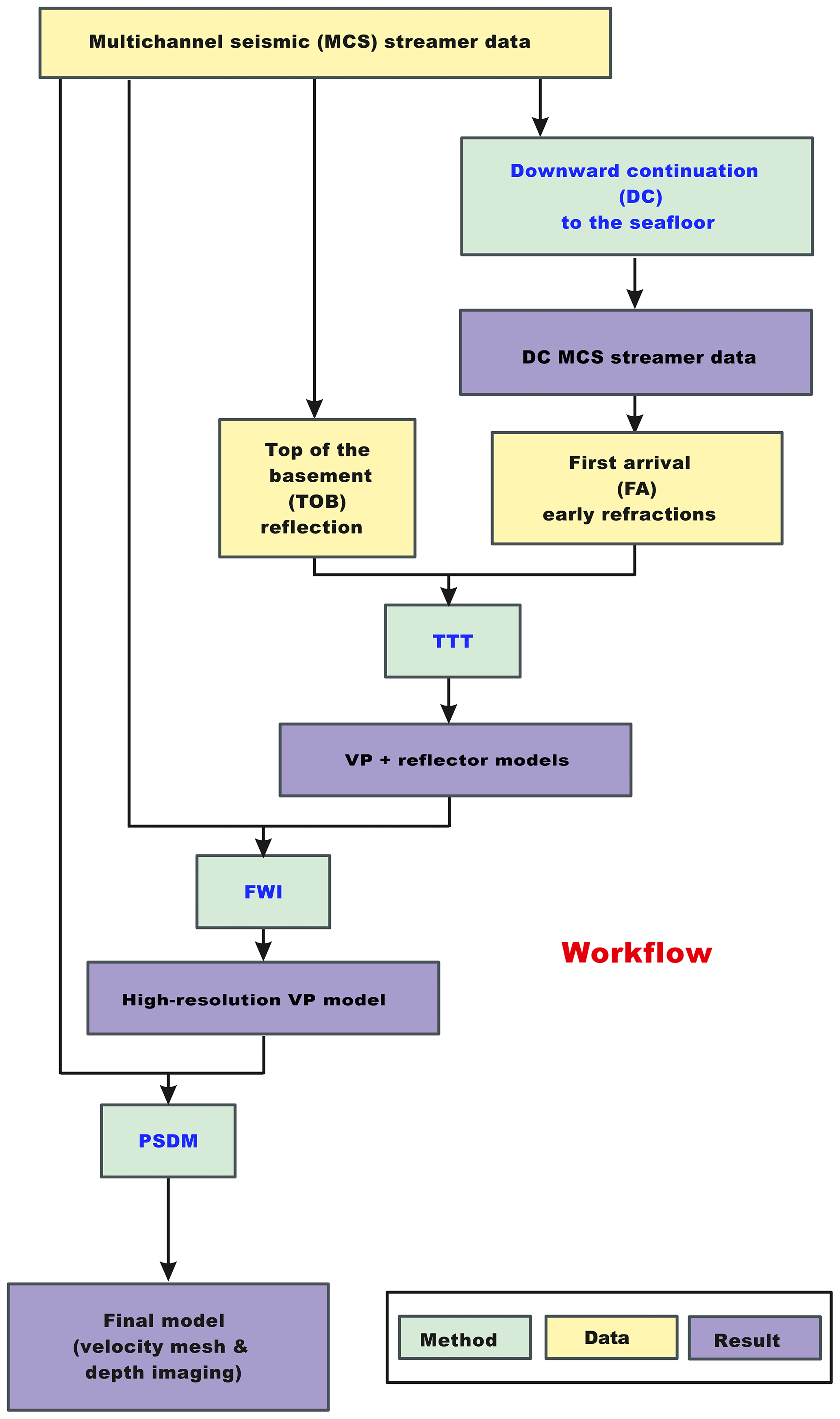
Figure 1 General scheme of the workflow. We build the V_P model sequentially, from long to short scales, taking advantage of all the information contained in our data. We apply the different techniques referred to in the text (DC, TTT, FWI, and PSDM) to obtain a high-resolution image of the subsurface.

2.1 Wave equation datuming (downward continuation)

As stated in the introduction, refractions are essential to build a macro-velocity model with the correct low-wavenumber content on it. As MCS acquisition systems have a limited offset (Fig. 2a), the first arrivals in deep-water environments are typically dominated by the direct wave as well as reflections, whereas refractions are hidden behind these phases (Fig. 2b). Several methods have been proposed to recover refracted signals by changing the plane of the acquisition geometry (e.g. Schuster and Zhou, 2006; Vrolijk et al., 2012; Wapenaar et al., 2014; Cho et al., 2016). The goal of wave equation datuming and, particularly, of DC, is to extrapolate the recorded data to a virtual datum surface so that refractions can be retrieved as first arrivals. The technique used here to back-propagate the recorded data follows the steps proposed by Berryhill (1979, 1984) and the scheme of McMechan (1982, 1983). This procedure is easy to implement and can deal with spatial velocity variations within the water column and irregular datum surfaces, which are often located at the seafloor (Fig. 2c).

Figure 2 (a) Scheme of a streamer acquisition geometry of a marine MCS experiment showing the main element as well as the paths of the seismic phases that can be recorded in the streamer hydrophones, where $z_{j}j=\mathrm{0},\mathrm{1},\mathrm{\dots }$ defines the depth of each layer, $v_{j}j=\mathrm{0},\mathrm{1},\mathrm{\dots }$ its V_P, and $i_{{\mathrm{crit}}_j}j=\mathrm{0},\mathrm{1},\mathrm{\dots }$ its critical angle. Green line is the direct water wave, blue and purple dotted lines are refracted ray paths in different interfaces, and its corresponding reflected ray paths are the pink and red dashed lines respectively. (b) Example of a synthetic shot gather recorded using a streamer-type geometry, as the one that is shown in (a). Each trace in the record section corresponds to a seismogram recorded at increasing source–receiver offset. Refractions are not visible, so they cannot be identified, and travel times cannot be used for velocity modelling. (c) Scheme of the virtual set-up to be simulated after DC. In this case, both sources and receivers are located at the seafloor. Green line is the direct water wave, blue line is the head wave that travels through the seabed interface, and dotted purple and red dashed lines are respectively the refracted and reflected ray paths of an interface of the subsurface. (d) Example of a synthetic shot gather recorded using the virtual geometry set-up shown in (c). Refractions are visible as first arrivals from zero offset.

The idea is eliminating the effect of the water layer by simulating a sea bottom acquisition (both sources and receivers). Without the water layer, the direct-wave signal and the seafloor reflections disappear, and the critical distance is reduced to zero offset. Thus, the virtual recordings contain early refractions visible as first arrivals (e.g. Fig. 2d).

In 2-D, the recorded wave field can be expressed as

$$\begin{array}{}\text{(1)}& \mathbf{S}(x_{\mathrm{s}},z_{\mathrm{s}};t)\cdot \mathbf{G}(x_{\mathrm{s}},z_{\mathrm{s}};x_{\mathrm{r}},z_{\mathrm{r}};t)=\mathit{u}(x_{\mathrm{r}},z_{\mathrm{r}};t),\end{array}$$

where t represents the time, x and z the horizontal and vertical spatial coordinates, S the source signal, G the Green's function that defines a forward wave field extrapolation process in a heterogeneous subsurface observed at (x_r,z_r) from a source at (x_s,z_s), and u is the seismic trace. In the streamer configuration (Fig. 2a), there are two contributions of the wave propagation through the water column that can be removed from the data by applying wave equation datuming. Following the matrix operator notation used by Berkhout (1981, 1997a, b), the true two dimensional (2-D) wave field propagation from sources to receivers is also formulated here by means of matrices but divided into three equations, each considering a different part of the total trajectory of the wave field, as

$$\begin{array}{}\text{(2)}& {\displaystyle }{\mathbf{S}}^{\mathrm{T}}(x_{\mathrm{s}},z_{\mathrm{s}};t)\cdot {\mathbf{G}}_{\mathrm{d}}(x_{\mathrm{s}},z_{\mathrm{s}};x_{\mathrm{d}},z_{\mathrm{bat}};t)={\mathit{u}}_{\mathrm{d}}^{\mathrm{T}}(x_{\mathrm{d}},z_{\mathrm{bat}};t),\text{(3)}& {\displaystyle }{\mathit{u}}_{\mathrm{d}}^{\mathrm{T}}(x_{\mathrm{d}},z_{\mathrm{bat}};t)\cdot {\mathbf{G}}_{\mathrm{e}}(x_{\mathrm{d}},z_{\mathrm{bat}};x_{\mathrm{u}},z_{\mathrm{bat}};t)={\mathit{u}}_{\mathrm{u}}^{\mathrm{T}}(x_{\mathrm{u}},z_{\mathrm{bat}};t),\text{(4)}& {\displaystyle }{\mathit{u}}_{\mathrm{u}}^{\mathrm{T}}(x_{\mathrm{u}},z_{\mathrm{bat}};t)\cdot {\mathbf{G}}_{\mathrm{u}}(x_{\mathrm{u}},z_{\mathrm{bat}};x_{\mathrm{r}},z_{\mathrm{r}};t)={\mathit{u}}^{\mathrm{T}}(x_{\mathrm{r}},z_{\mathrm{r}};t),\end{array}$$

where Eq. (2) corresponds to the downward propagation (G_d) from the source (S) surface (x_s,z_s) to the seafloor (x_d,z_bat) through the water column; Eq. (3) describes the effects of the wave propagation through the Earth's subsurface (G_e) for an acquisition system deployed at the seafloor from an incoming wave field at (x_d,z_bat) to an outcoming wave field at (x_u,z_bat), and Eq. (4) represents the upward propagation (G_u) from the seafloor (x_u,z_bat) to the recording surface (x_r,z_r) through the water media; ${\mathit{u}}_{\mathrm{d}}^{\mathrm{T}}$, ${\mathit{u}}_{\mathrm{u}}^{\mathrm{T}}$, and u^T represent the pressure field expressed at its corresponding datum surface as a row vector, “T” being the transpose symbol. The G_d and G_u operators are equal only if sources and receivers are located at the same horizontal coordinates and thus the downward and upward vertical propagation follow the same path.

Here the inverse extrapolation follows the boundary value migration (BVM) scheme of McMechan (1982, 1983). In this case, the inverse extrapolation is described by the source, wave equation and boundary conditions used. The source function through time is formed by the observed wave field, which is introduced in the 2-D model plane sequentially and backwards in time as a boundary value. The wave field transferred from the seismogram to the model at each time step is taken as an equivalent source. The complete seismogram is used; thus no preselection and arrival identification are needed. Prior to re-datuming, we (1) deleted noisy channels, (2) applied Butterworth 1/3-40/60 filtering, and (3) muted direct arrival. We did not apply amplitude corrections. The proper source spacing and optimal recording time step are the ones that avoid aliasing issues and grid dispersion and reduce the effects caused by the discrete approximation of the wave field.

The inserted wave field is propagated back in time following the acoustic wave equation solved by the forward extrapolation scheme (Dagnino et al., 2016). The following 2-D acoustic differential equation,

$$\begin{array}{}\text{(5)}& \begin{array}{rl}{\displaystyle \frac{\mathrm{1}}{\mathit{\kappa }(x,z)}}{\displaystyle \frac{{\partial }^{\mathrm{2}}\mathit{u}(x,z;t)}{\partial t^{\mathrm{2}}}}& +\mathrm{\nabla }\cdot \left({\displaystyle \frac{\mathrm{1}}{\mathit{\rho }(x,z)}}\mathrm{\nabla }\mathit{u}(x,z;t)\right)\\ & =s(x,z;t),\end{array}\end{array}$$

where x is the horizontal space coordinate, z the depth or vertical space coordinate, t the time, u the pressure wave field, s the source signal, κ the compressibility, and ρ the density of the medium, is implemented in a recursive and explicit finite difference (FD) scheme of the two-way wave equation in the space–time domain (Dagnino et al., 2016). The inverse extrapolation is the reverse of the forward propagation because the recorded traces that act as sources (s) are reversed in time. This is because for a lossless medium, the wave equation is symmetric in time (reversible) and the Green's function is reciprocal. The idea is that reflectors exist in the Earth at places where the onset of the downgoing wave is time coincident with an upcoming wave (Claerbout, 1976). Thus, the true forward propagation of the wave field is compensated for by the inverse extrapolation that sends the recorded energy back through the same paths but in the opposite direction. The progressive focusing in time and space of the wavefronts makes it possible to recover the wave field at a later stage. Hence, the re-datumed wave field is directly imaged at the new surface depth along the extrapolation time. A multi-shooting technique is applied to back-propagate the wave field from all the recorded seismograms at once, increasing the signal-to-noise ratio (SNR) and making the process more compact both in memory and computational time.

Unlike re-datuming approaches that use the Kirchhoff implementation (Berryhill, 1979, 1984; Shtivelman and Caning, 1988; Arnulf et al., 2011), the computation of extrapolated data at intermediate depth levels is needed. Despite the fact that it increases the computational complexity as compared with the Kirchhoff method (Arnulf et al., 2014), the wave equation imaging allows including laterally and vertically variable water velocity, in contrast with other techniques in which the water velocity is considered constant (Cho et al., 2016) or needs a specific ray tracing (Shtivelman and Caning, 1988). Recursive extrapolation makes that spatial velocity variations can be handled properly. To define the 2-D water velocity model we use in situ oceanographic measurements of water properties obtained with expendable bathy-thermographic (XBT) probes. We have also tested the effect of the water velocity model used to DC the shot gathers versus the travel-time picks. In our area of study the velocity changes in the water layer are small (<20 km s⁻¹), so considering either a realistic or a homogeneous model has a minor effect on the first arrival travel-time picks, smaller than the travel-time picking uncertainty (±0.035 s). Moreover, the new virtual positions do not necessarily have to be in a flat surface or at several metres above the seafloor surface as in other studies (e.g. Harding et al., 2016); here the new virtual surface is the seafloor relief, itself extracted from bathymetric data. In contrast to Harding et al. (2016), who use the DC data to perform FWI, we only use first arrival travel times to perform TTT, so surface-related effects do not affect the inversion results here. The main drawback of this DC strategy is the computational cost, worse wave field reconstruction in the far offsets caused by the truncation of the recorded data, and potential artefacts due to propagation effects.

In the inverse extrapolation process, complex-frequency-shifted perfectly matched layers (CFS-PML) (Zhang and Shen, 2010) are imposed as absorbing boundary conditions to avoid spurious reflections in all model boundaries that may cause interference and mask the correct seismic phases. The only exception is the time-dependent boundary values associated with the equivalent sources.

In summary, the main steps of the DC approach are the following: first, we back-propagate the shot gathers through the water layer from the receiver positions to a virtual surface located at the seafloor. Then, we sort the resulting virtual seismograms into common receiver gathers. After that, we back-propagate the receiver gathers through the water layer, this time from the virtual surface to the source positions, in the opposite direction to its true trajectory. Finally, we re-sort the resultant wave field in the original shot gather domain (Fig. 2d). The rearrangement of the data is possible because of the reciprocity principle, so that if source and receiver have identical directional characteristics, then interchanging the positions of sources and receivers yields the identical seismic trace (Berryhill, 1984).

The final virtually recorded wave field with sources and receivers located at the seafloor can be expressed as

$$\begin{array}{}\text{(6)}& {\mathbf{S}}^{\mathrm{T}}(x_{\mathrm{s}},z_{\mathrm{s}};t)\cdot {\mathbf{G}}_{\mathrm{e}}(x_{\mathrm{s}},z_{\mathrm{bat}};x_{\mathrm{r}},z_{\mathrm{bat}};t)={\mathit{u}}_r^{\mathrm{T}}(x_{\mathrm{r}},z_{\mathrm{bat}};t).\end{array}$$

Because the re-datumed wave field (u_r) at (x_r,z_bat) is built by using finite, discrete, and single-sided recordings, it is not the pressure wave field that would be recorded by performing the experiment with the virtual geometry set-up. Moreover, the energy coming from the direct and surface waves is not included. In general, the amplitude of the resulting wave field is reduced due to the energy loss through the absorbing model boundaries during the inverse extrapolation process. Therefore, amplitude is not preserved as in other re-datuming approaches (Schuster and Zhou, 2006) and its attenuation factors are related to geometrical spreading and transmission losses. As amplitudes are affected by the re-datuming process, it is not straightforward performing FWI using DC data. However, arrival times of the different phases are correct (which is our main objective) if the V_P model of the water layer is accurate enough. A better approximation of the true wave field, and thus a better result, would be achieved using denser and larger arrays. For sparse data sets the re-datumed arrivals would be less focused due to a larger amplitude loss and noise effects, but it would nevertheless be correctly located.

The accuracy of the resulting wave field also depends on the precision of the forward solver. The numerical algorithm (Dagnino et al., 2016) uses a Runge–Kutta method of fourth order in time (Lambert, 1991) and a sixth-order approximation in space discretized with a staggered grid (Virieux, 1986). It employs the extrapolated output as input for the next extrapolation step (recursively) plus four weighted average increments.

Another effect that can affect the result is the presence of artefacts such as diffraction tails located at the edges of the array and therefore where the observed wavefronts are truncated. These artefacts are due to the finite aperture of the recording system. Their effects are larger for small aperture set-ups, where they can interfere with the energy focusing in the new datum surface and mask the true arrivals. Moreover, the finite aperture of the acquisition array causes a non-uniform illumination of the wavefronts, which results in energy mitigation near the recording limits. Finally, the resulting extrapolated wave field is also influenced by numerical dispersion, which attenuates high frequencies as it travels backwards in time through the medium. Thus, the spectrum of the frequency bandwidth of the data is reduced due to the Earth effect that acts as a filter (Berkhout, 1997a, b).

2.2 Joint refraction and reflection travel-time tomography

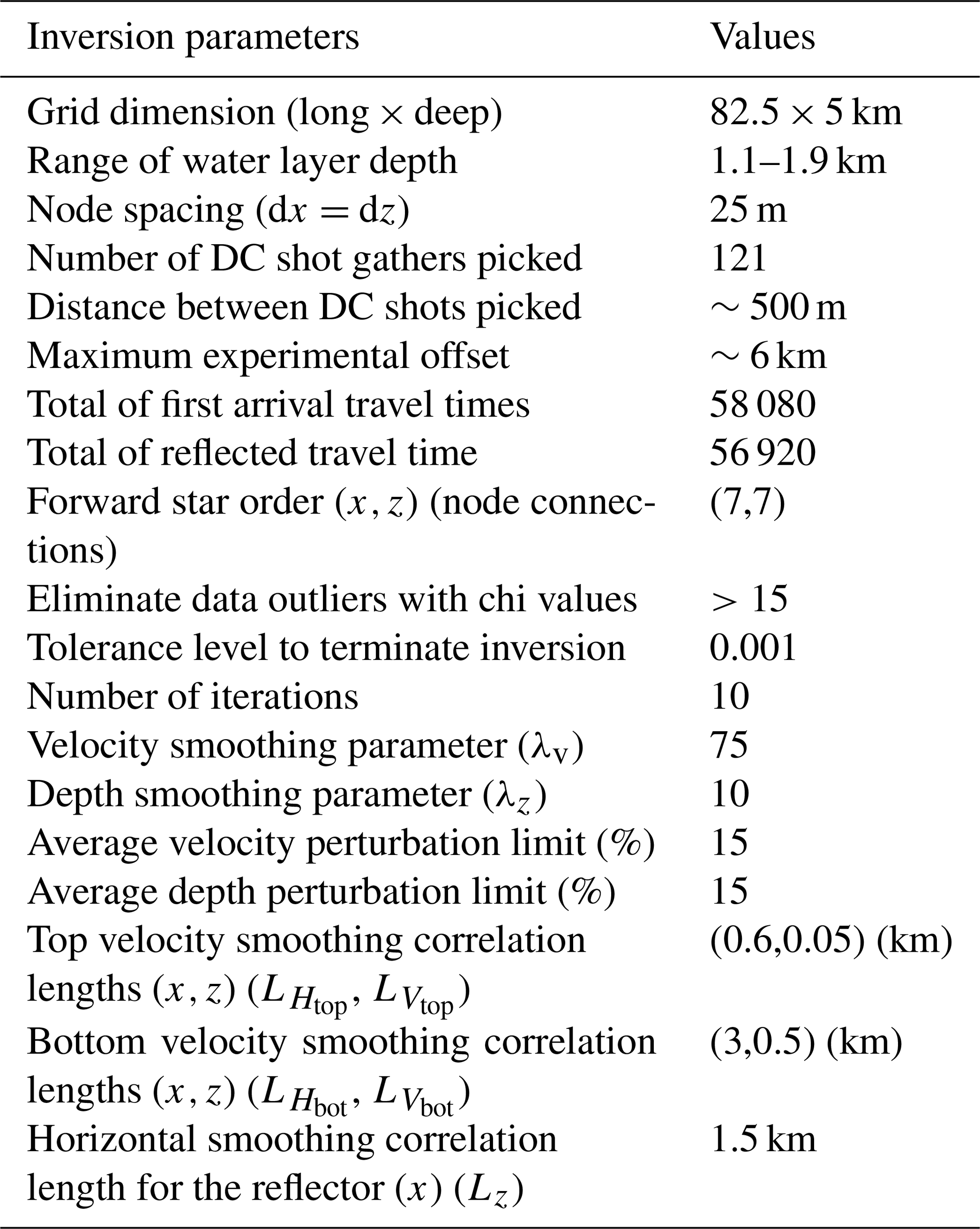
The goal of this step is to obtain a reference V_P model by TTT of some predefined seismic phases; in particular, we combine first arrivals identified at the virtual DC recordings with reflections recorded for the original MCS data. Therefore, the data input file contains both types of travel-time picks, each with their corresponding source–receiver positions. In the case of DC arrivals, the 2-D coordinates will be the ones in the virtual surface, but for the reflections they will be at the actual location of the air gun source and of the individual streamer channels. Further details for our particular study area and experiment are presented in Sect. 4.2. As a rule of thumb, it is considered that V_P models obtained by TTT are correct to a depth that is about a half of the maximum experimental offset.

We use a version of the TOMO2D code (Korenaga et al., 2000) modified by Begovič et al. (2017) to enable locating both sources and receivers within the water layer so as to invert streamer data. A two-dimensional V_P model is parameterized in our study as a regular mesh hanging from the seafloor, i.e. the model is limited to the subsurface medium and does not include the water layer. Propagation velocity in the water layer is fixed to 1.5 km s⁻¹. Arrival time differences using a realistic water V_P model are much smaller than the expected data misfit, typically several tens of milliseconds. A 1-D floating reflector is defined along the profile. This means that it is parameterized as a node array that is independent from the velocity mesh, and both reflector array and velocity mesh can be spatially variable. Travel times for given V_P and reflector depth models are computed using a ray tracing strategy that combines the graph method (Moser, 1991) with a subsequent ray bending refinement (Moser et al., 1992).

The partial derivatives of travel-time residuals with respect to velocity (for first arrivals and reflections) and reflector depth (only for reflections) are introduced in the Fréchet matrix with additional regularization constraints (smoothing, damping). Thus, this interface depth model is inverted simultaneously with the V_P model. The inverse problem to iteratively update the V_P and depth models is solved using the sparse matrix solver of the LSQR (least square root) algorithm of Paige and Saunders (1982). The difference between observed and synthetic travel times is iteratively minimized as a least-squares problem until a stopping criteria is fulfilled. Regularization constraints (smoothing and damping) are applied to stabilize the minimization process avoiding singularity of the matrix. For further details, see Korenaga et al. (2000) and Meléndez et al. (2015).

2.3 Full-waveform inversion

The last inversion step of the proposed approach is using the V_P model obtained by TTT as initial one for adjoint-state FWI. In this case, we use the original seismograms recorded by the MCS system as input to refine the V_P model. As in the case of the DC, the FWI code uses the acoustic domain FD solver of Dagnino et al. (2014, 2016) for the forward- and back-propagation of the wave equation.

2.3.1 Forward problem

For the forward problem, we consider the 2-D acoustic wave equation in the time domain expressed in the form that appears at Eq. (5) to simulate the synthetic pressure wave field. The code includes CFS-PML (Zhang and Shen, 2010) as boundary conditions, and we use 25 layers on the left, bottom, and right boundaries to eliminate numerical reflections and a free surface at the top of the model that represents the water–air discontinuity. The optimal temporal step to solve the forward problem fulfils the usual Courant–Friedrich–Lewy stability condition to avoid instabilities in the PML (Dagnino et al., 2014). To estimate the source for the first iteration we use a Ricker wavelet with central frequency of 20 Hz. Then the source wavelet is inverted at each iteration as proposed by Pratt (1999) prior to velocity inversion, so the updated source signature is used in the subsequent iterations (Dagnino et al., 2016). The source signature is calibrated and inverted for all the individual shots up to 0.5 km offset. The initial (T/6) and final (6T) oscillations, where T is the period of the source signal, are removed to avoid the introduction of noise in the synthetic data.

2.3.2 Inverse problem

The goal of the inversion is to find the parameters m, in our case V_P, that minimize the discrepancy or misfit between some predefined waveform attributes of the observed (u^o) and synthetic (u^s) seismic traces at each iteration (Jiménez Tejero et al., 2015). We use the classical L2-waveform objective function (χ) that is built as the least-squares norm of the corresponding misfit (Tarantola, 1987) for a source as follows:

$$\begin{array}{}\text{(7)}& \mathit{\chi }=\sum _{\mathrm{r},\mathrm{t}}{\displaystyle \frac{{\left({\mathit{u}}^{\mathrm{s}}(x_{\mathrm{r}},z_{\mathrm{r}};t)-c_{\mathrm{r}}{\mathit{u}}^{\mathrm{o}}(x_{\mathrm{r}},z_{\mathrm{r}};t)\right)}^{\mathrm{2}}}{\mathrm{2}}},\end{array}$$

where x_r is the receiver position, t the time, and c_r the calibration term. The calibration term is calculated independently for each source–receiver as in Dagnino et al. (2016), but fixing the sea bottom reflection instead of the direct water wave. This term is useful to correct the source signature changes due to an irregular bathymetry and the inhomogeneous source directivity. The wave field of each shot gather is resampled to fit on the finite difference grid. The synthetic data for the misfit calculation is simulated solving the forward problem previously explained in a reference model and its updates.

The acoustic 2-D forward modelling code compensates for the actual 3-D amplitude decay of the field data multiplying the field data by $\sqrt{t}$ (Hicks and Pratt, 2001; Dagnino et al., 2016) before the calculation of the residuals. Moreover, the energy of the shots is normalized dividing it by the total source energy to overcome problems due to elastic effects. The density model of the subsurface used for the inversion also affects the reflectivity part of the data set, so it is important to interpret the reflectors not only as velocity contrasts. In our case, it is updated after the inversion of each frequency band using the V_P model obtained at the previous iteration and the Nafe–Drake (Ludwig) experimental relationship (Mavko et al., 1998).

The following step consists of updating the model in the direction where the misfit decreases. For this purpose, we calculate the gradient of the misfit following the adjoint-state method proposed by Lailly (1983) and Tarantola (1984). The adjoint field is obtained by back-propagating the residuals in time for each receiver position. The adjoint source is calculated as $\mathit{f}(x,z;t)=-{\mathrm{\nabla }}_{u^s}\mathit{\chi }$.

The gradient of the objective function with respect to the model, ∇_κχ, is computed by convolution of the forward-propagated wave field of the source term and the adjoint or back-propagated wave field of the residuals from the receiver location (Tarantola, 1984).

$$\begin{array}{}\text{(8)}& {\mathrm{\nabla }}_{\mathit{\kappa }}\mathit{\chi }=\sum _{\mathrm{s}}{\displaystyle \frac{\mathrm{1}}{\mathit{\kappa }(x,z)}}\underset{t}{\int }{\displaystyle \frac{\partial \mathit{u}(x,z)}{\partial t}}{\displaystyle \frac{\partial \mathit{f}(x,z)}{\partial t}}\end{array}$$

Because of non-linearity, the gradient can point toward a local minimum. In the FWI code, a gradient-based preconditioning concentrates model updates in the regions where the gradient is more reliable. Moreover, it also adds a weighting to compensate for the amplitude decay of the signal away from the source. Furthermore, the gradient is balanced to reduce its sensitivity to the presence of “spikes” with a smoothing regularization based on a 2-D low-pass zero-phase Butterworth filter. Details on the gradient preconditioning techniques can be found in Dagnino et al. (2014, 2016).

We use the steepest descendent (SD) approach in the optimization problem because it has particularly low sensitivity to noise. The step used to find the direction in the model space where the misfit function locally decreases, is just the opposite of the gradient in the SD approach, ${\mathit{p}}_i=-\mathrm{\nabla }{\mathit{\chi }}_i$. In the FWI algorithm, we use a normalized search direction. Then, the optimal step length (α_i) is determined by imposing ${\mathit{\alpha }}_i={min}_{c>\mathrm{0}}\mathit{\chi }({\mathit{m}}_i+c{\mathit{p}}_i)$. The final step is obtained after acquiring the minimum of a polynomial approximation over three steps calculating the search direction of the misfit function, p_i. Then, the model can be updated as ${\mathit{m}}_{i+\mathrm{1}}={\mathit{m}}_i+{\mathit{\alpha }}_i{\mathit{p}}_i$.

A multi-scale approach where frequency bands are inverted sequentially, from low to high frequencies (Bunks et al., 1995), is applied to reduce the risk of falling into a local minimum and to add details to the model progressively. In particular a low-pass Butterworth filter is applied to the data, which allows us to solve different frequency bands of the same data at each iteration, restricting the inversion to a limited bandwidth. Implementing this strategy mitigates the non-linearity because the objective function is smoothed when the data are filtered. High wavenumbers are then incorporated sequentially into the model's successive iterations. The maximum number of iterations per frequency step is fixed to 10. An additional stopping criterion that we use in the inversion is the Arminjo rule (Nocedal and Stephen, 2006) when changes are <0.01.

2.4 Pre-stack depth migration

We apply a 2-D Kirchhoff depth migration to image the subsurface structures directly at depth by using the V_P models obtained and the high-frequency content of the data set. The migration module applied is part of the Seismic Unix platform. We use the sukdmig2d command for the data migration. The travel timetable required for the depth migration is obtained with the rayt2d command, which calculates the 2-D ray tracing along the V_P model.

3 Study area and data set

The field data used to test the described approach correspond to an experiment conducted in the Alboran Sea, a complex basin located in the westernmost Mediterranean (Fig. 3) (Booth-Rea et al., 2007, 2018). The target of this survey was to image the structure and properties of the sediment units and the nature of the uppermost basement.

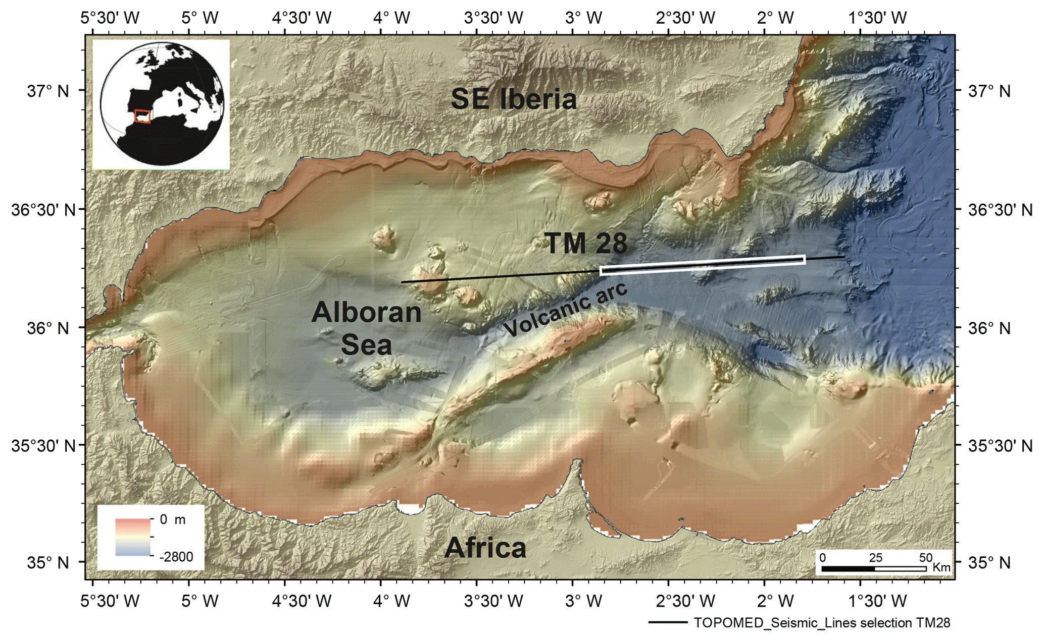
Figure 3 Relief map of the study area (Ballesteros et al., 2008; Gràcia et al., 2012; Gómez de la Peña et al., 2016). The field data used in the test correspond to the white box along the TM28 profile.

The seismic records used in this study were collected in 2011 on board Spanish R/V Sarmiento de Gamboa, as part of the TOPOMED cruise. We select an 80 km long section of the TM28 profile that crosses the central and deepest part of the basin, across a volcanic arc (Gómez de la Peña et al., 2018), to test the approach. The input data consist of series of seismograms (traces) recorded with a 6 km long streamer (Fig. 4). The streamer has 480 channels with a group interval of 12.5 m. The length of the trace record used is 8 s and the time sampling is 2 ms. In total, we use 1517 air gun shots with an average spacing of 50 m. The source power was 4600 cubic inches, producing a central frequency of ∼20 Hz. The system was towed at a depth of 10 m, and the nearest-offset distance was 203.7 m. The early arrivals in the streamer recordings are dominated by the shallow near-vertical sediment reflections, as can be seen in Fig. 4. Hence, data preconditioning is essential to identify first arrivals and make the data set appropriate for TTT.

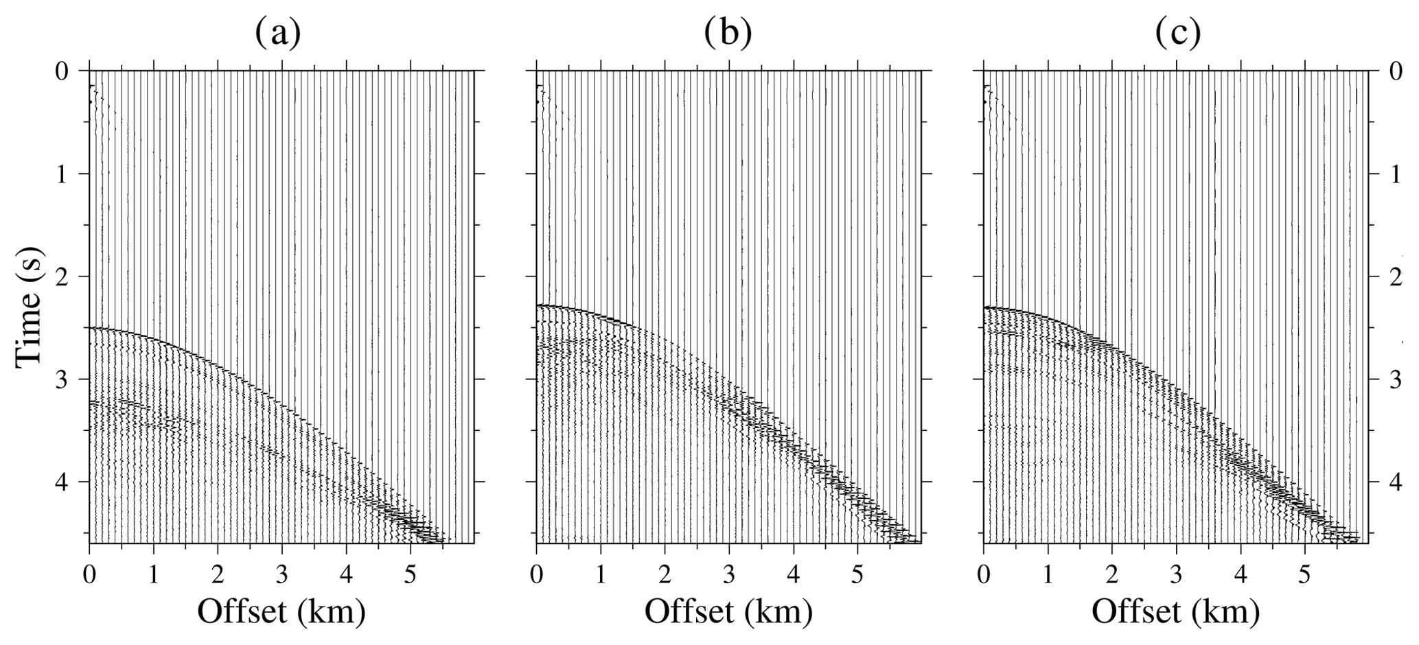
Figure 4 Decimated example of the field data set; only 10 traces in each kilometre are plotted (so 0.2 of the total) for clarity. From (a) to (c), shot locations are at 171.1, 138.7, and 112.5 km along the profile.

4 Results

Here we show the results after applying each step of the modelling strategy described in the previous sections (see Fig. 1). We work under the premise that we have no a priori information on the structure and properties of the subsurface, so the goal is to recover all the possible information on the V_P model from the MCS data alone. Before starting our processing and modelling workflow, we apply a 2-D band-pass minimum-phase Butterworth filter to the data set for swell noise removal. The low cut and high cut of the band-pass filter are 2 and 60 Hz respectively. The DC result of the streamer recordings is first shown to make the early refractions visible as first arrivals. Then, a macro-velocity model is obtained by joint refraction and reflection TTT, which is then used as initial model to perform FWI starting at ∼6 Hz, the lowest signal frequency available in data set. Afterwards, we perform a PSDM of the recorded data using the 2-D V_P models obtained by TTT and by FWI.

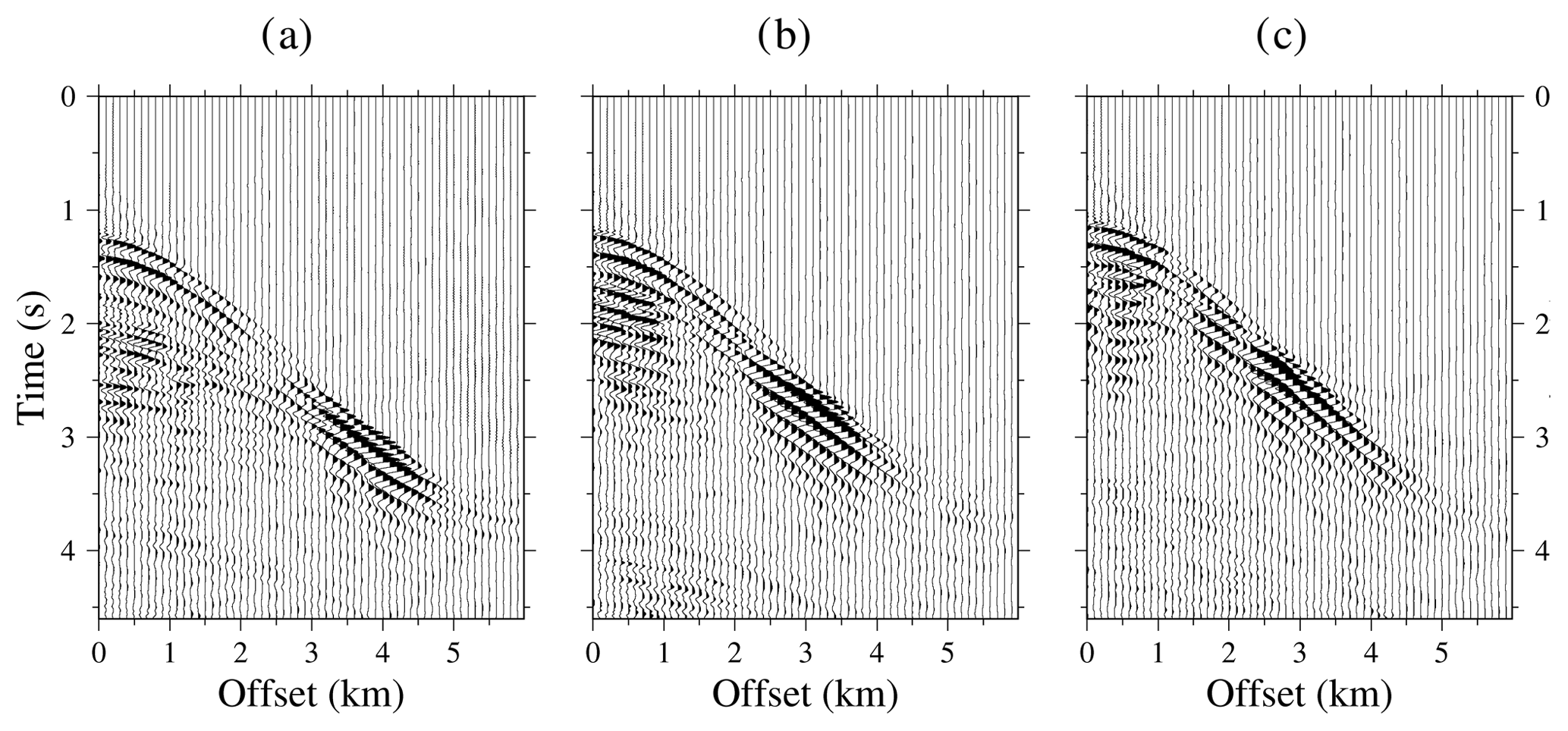
Figure 5 Seismic data obtained after the first DC step of the streamer shots recorded in the TOPOMED cruise. The wave fields are displayed for every fifth trace (so 10 traces each kilometre, 0.2 of the total). From (a) to (c), shot locations are at 171.1, 138.7, and 112.5 km along the profile.

4.1 Downward continuation results

We compute the data re-datuming by wave equation DC of the streamer recordings to the seafloor surface. Figure 5 shows the result after the first step of the DC for three shot gathers derived using the full wave field of each shot and a heterogeneous water layer model built as explained in the Methodology section. The grid size in both the x and z direction is 12.5 m. We image the wavefronts of all the seismic events recorded in the streamer traces reconstructed by the solver after its back-propagation to the virtual receiver positions in the correct reversed time (i.e. the OBS (ocean bottom seismometer)-type acquisition setting). In this way, we recover several first arrivals that were obscured in the original recordings. However, the main first arrival along the recordings is still the seafloor reflection.

In the second step, we re-sort the virtual OBS-type wave field in receiver gathers, and then, the data from all shot gathers are combined to construct the final virtual shot gather. Figure 6 shows the final result for the three shot gathers also shown in Fig. 5. The DC has collapsed the seafloor reflection towards a single point, so refractions from shallow subsurface can now be identified and tracked as first arrivals from zero offset. First arrivals are more difficult to identify at long offsets because of amplitude attenuation and the appearance of diffraction tails. Lower panels (d–f) in Fig. 6 show the first arrivals used as input for the TTT (blue dots).

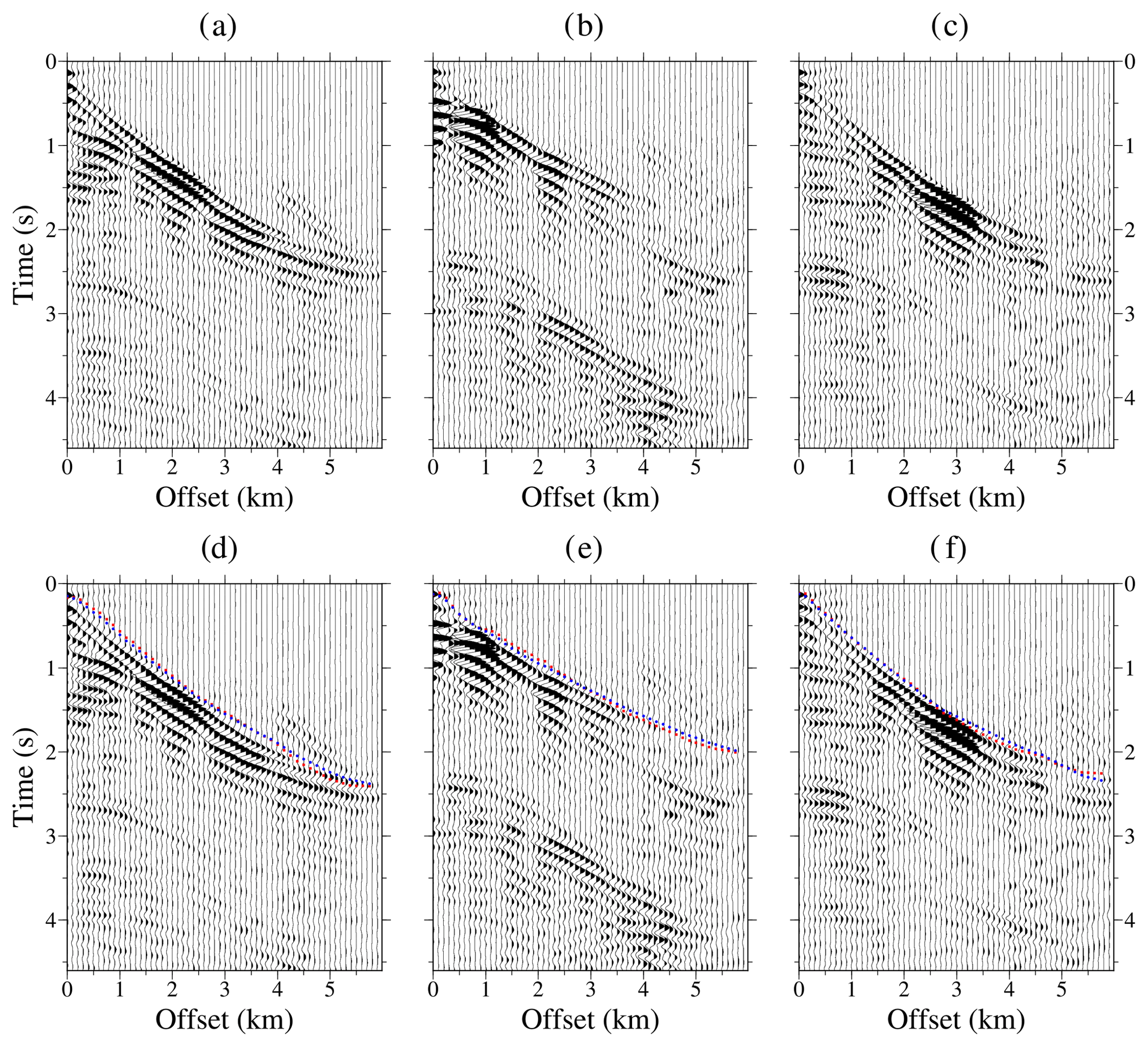
Figure 6 Seismic data obtained from the DC of the streamer shots recorded in the TOPOMED cruise. Only 10 traces each kilometre are plotted (so 0.2 of the total) for clarity. From left to right, shot locations are at 171.1, 138.7, and 112.5 km along the profile. Panels (d)–(f) show shots (a)–(c) together with first arrivals used as input for the TTT (blue dots) and the first arrivals simulated with the TTT model (red squares).

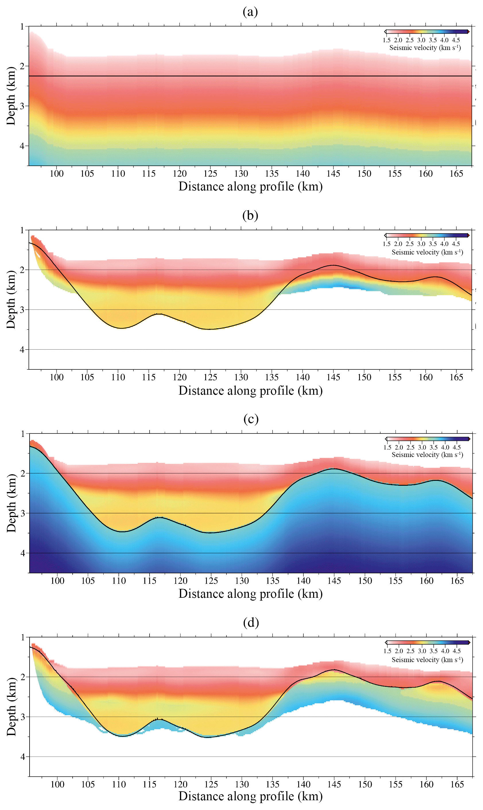
Figure 7 (a) Initial V_P and TOB models for the first inversion step. (b) Inverted V_P and TOB models after the first inversion step using (a) as initial ones. (c) Initial V_P and TOB models for the second inversion step. (d) Inverted V_P and TOB models after the second and final inversion step using (c) as initial ones. Both inversion steps use the same inversion parameters in Table 1, and the data set is made up of the first arrivals of the DC shot gathers and the reflected phase of the TOB discontinuity identified in the original streamer records. Only the ray-covered areas of the model, where the derivative weight sum (DWS) is not zero, are plotted. The thick black line corresponds to the location of the TOB.

Table 1 Relevant inversion parameters used in the TTT.

4.2 Joint refraction and reflection travel-time tomography results

The inversion parameters used in the TTT are shown in Table 1. We do not use the entire data set to reduce computational burden, but all receivers are used to ensure data redundancy. The selected reflection corresponds to the top of the basement (TOB), which is a clear event (e.g. see Fig. 9). Reflection travel times are picked from MCS common midpoint gathers where it is a bright continuous reflection, which is also interpreted at the same time in a fully processed stacked image (Fig. S1 in the Supplement). The source and receiver positions were projected to a straight line defined between first and last shots, preserving their offset distance. Correlation lengths for the velocity model are set at the top and bottom nodes of the grid and are linearly interpolated for the intermediate nodes. The velocity gradient is stronger in the vertical direction, so the vertical correlation lengths are selected to be shorter than the ones defined in the horizontal direction. Our inversion process follows the layer-stripping strategy as described in Meléndez et al. (2015). In the first inversion step, the initial TOB depth model is a flat boundary located at 2.25 km depth, and the initial V_P model follows the linear function of depth from the seafloor $V_{\mathrm{P}}\left(z\right)\left[\mathrm{km}{\mathrm{s}}^{-\mathrm{1}}\right]=\mathrm{1.61}+\mathrm{0.72}\cdot z\left[\mathrm{km}\right]$, increasing from 1.61 km s⁻¹ at the seafloor to 4.13 km s⁻¹ at a depth of 3.5 km below the seafloor (Fig. 7a). In the second inversion step we use the inverted TOB from the first step (Fig. 7b) as initial TOB depth model and the same data set and inversion parameters. Regarding the V_P model, we build a new initial model that is equal to the V_P model above the TOB obtained in the first step, whereas below it, V_P is defined as $V_{\mathrm{P}}\left(z\right)=V_{\mathrm{TOB}}+(z-z_{\mathrm{TOB}})\cdot \frac{(V_{z_{\mathrm{f}}}-V_{\mathrm{TOB}})}{(z_{\mathrm{f}}-z_{\mathrm{TOB}})}$, varying from 3.6 km s⁻¹ at the TOB interface (V_TOB) to 6 km s⁻¹ ($V_{z_{\mathrm{f}}}$) at a depth of 8.6 km below the seafloor (z_f) (Fig. 7c). The goal of the layer-stripping strategy is to recover the sharp velocity contrast at the sediment–basement reflecting boundary, which might otherwise appear as a smooth velocity gradient, contributing also to the improvement of the deepest part of the model.

The final macro-velocity model is presented in Fig. 7d. The joint refraction and reflection TTT allows recovering the long-wavelength geometry of the sharp sediment–basement boundary. The ray coverage of the model inversion is quantified by the derivative weight sum (DWS) (Toomey et al., 1994) (Fig. 7), and it is influenced by the geometry of the experiment and the subsurface velocity distribution. Thus, ray coverage decreases to the edges of the model and with depth, and it is denser beneath the source locations. The model is generally well constrained in the central part that is covered by both refractions and reflections, whereas the lateral areas mapped only by reflections are subject to a higher degree of velocity–depth ambiguity. In the central area, the overall trend is an increase in velocity with depth, from ∼1.6 km s⁻¹ at the seafloor to ∼4.0 km s⁻¹ at the bottom. The results indicate that a high-velocity anomaly (>3.5 km s⁻¹) is located at ∼115 km distance and ∼3 km depth. Slower velocities are obtained at shallower depths below the TOB. The velocity contrast that accurately follows the geometry of the TOB is delimiting steeply dipping discontinuities. As an example, we show that on the left-hand side of the profile in Fig. 7d the basement is located just below the seafloor (∼200 m with respect to the seafloor), whereas ∼15 km further along the profile the basement position is at a depth of ∼3.5 km. On the other side, the geometry of the TOB is gently wavy around an average depth of 2 km. The TOB boundary marks strong velocity changes with a velocity jump of ∼0.5 km s⁻¹ between sediment and basement velocities (>2.7 km s⁻¹).

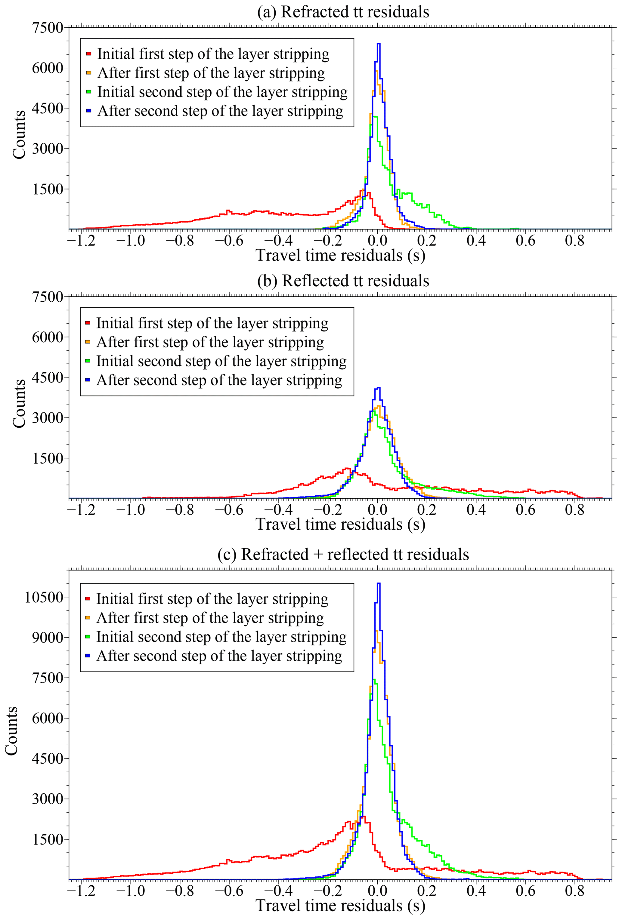
Figure 8 Histogram of travel-time residuals. Panel (a) shows only the residuals of the refractions obtained with the initial (red), after the first inversion step (orange), initial for the second inversion step (green), and final (blue) models. Panel (b) shows only the residuals of the reflections obtained with the initial (red), after the first inversion step (orange), initial for the second inversion step (green), and final (blue) models. Panel (c) shows the residuals of both phases (refractions and reflections) for the initial (red), after the first inversion step (orange), initial for the second inversion step (green), and final (blue) models. Travel time is indicated by “tt”.

Figure 8 shows histograms of travel-time residuals for three data groups after the first and last iterations of the two inversion steps of the layer-stripping strategy. The distributions of data misfit with the initial model (red lines) are asymmetric and wide for both refractions and reflections. After the first inversion step (orange lines), the distributions are symmetric and narrower with the highest pick around zero. At the initial stage of the second inversion step of the layer stripping (green lines), an increase in positive travel-time residuals is shown with respect to the distribution after the first step (orange lines) due to the insertion of higher velocities below the TOB to recover the sharp velocity contrast. Thus, the distributions (green lines) are slightly asymmetric and wider than after the first step of the layer stripping (orange lines). The final distributions of travel-time residuals (blue lines) are narrower than the previous ones and approach to a Gaussian centred at zero with the largest counts. This fact evidences the improvement of the velocity model, and therefore the corresponding travel-time fitting during the inversion. Lower panels (d–f) in Fig. 6 show the first arrivals for three DC shot gathers used as input for the TTT (blue dots) and the first arrivals recovered after TTT (red squares). The final velocity model in Fig. 7d shows a good convergence with root mean square (rms) residual travel times of ∼20 ms, which is of the order of the picking uncertainty (χ²≈1). In contrast, the initial rms before the inversion (Fig. 7a) is ∼420 ms.

Figure 9 Two-way time-transformed V_P and TOB models obtained after the joint DC refraction and streamer reflection TTT are shown superimposed on the time-migrated MCS image.

Moreover, to assess the reliability of the inversion results, we convert the velocity and TOB models to two-way time and superimpose the results on top of the time-migrated image (TMI) (Fig. 9). The figure shows that the TTT V_P and TOB models and the MCS image are both consistent, since both the velocity contrasts and the depth of the TOB are located in the same two-way time where the TMI displays important reflectivity changes and the TOB discontinuity. The good match validates our travel-time picks, given that neither the interpolation of the reflected picks or the inclusion of the far-offset first arrival DC travel times appear to introduce substantial artefacts or errors in the model. However, the TTT model lacks resolution compared to the time-migrated MCS image. It does not reproduce the sharp geometry and changes in amplitude of the anomalies in detail, such as the highs and lows of the TOB, the faults at the flanks, or the sediment layering seen in the TMI.

4.3 Full-waveform inversion results

After TTT, we perform FWI of the original streamer shot gathers starting from a smoothed version of the TTT V_P model of Fig. 7d. A total of 1512 shot gathers (>720 000 seismograms) are used for the inversion. The length of the traces is 4.6 s. In order to reduce computational costs, we invert sequentially four different sets of 378 shot gathers for each frequency band. Source and receiver positions are also projected to a straight line defined between first and last shots, preserving their offset distance. As in TTT, no decimation is applied to receiver sampling.

We apply a data preconditioning to emphasize reflections between the first arrival, typically the seafloor reflection, and its first multiple, using data windowing. We define a time window centred at the seafloor reflection. We identify this phase by using a maximum kurtosis and k statistics criterion (Saragiotis et al., 2002). We calculate the travel time of the seafloor reflection approximately using a water velocity of 1.5 km s⁻¹, the seafloor depth, and the source–receiver offset distance. When the first arrival is not found, for example due to a noisy channel, or the observed and simulated seismograms are cycle-skipped for the inverted frequency, then the trace is eliminated. The trace value is set to zero before the first arrival travel time, and after that it is balanced by a function defined as $\sqrt{t}$ to compensate for the amplitude decrease at depth. Finally, the trace is also set to zero after the travel time of the first multiple. Therefore, the gradient calculation focuses on information of the data set coming from the near-vertical reflections. Additionally, when the absolute difference between the maximum amplitudes of a field and its corresponding synthetic traces is higher than 3 times the maximum amplitude of the synthetic trace, it is considered to be a noisy channel and the trace is eliminated. Another issue to consider when comparing synthetic and field data is having a high signal-to-noise ratio (SNR), so each trace is stacked with its two neighbours at frequencies lower than 8 Hz.

We start the multi-scale FWI at 6 Hz. The maximum frequency inverted is 16 Hz. A frequency step of 0.5 Hz is applied at the beginning and 1 Hz at the final stages of the multi-scaling inversion. A total of 14 different frequencies in the multi-scaling strategy are inverted. The size of the space grid for the inversion ($\mathrm{d}x<\frac{{\mathit{\lambda }}_{\mathrm{inv}}}{\mathrm{5}}$) depends on the frequency step and the minimum velocity of the model, being smaller at high frequencies. The minimum and maximum velocities were constrained as gradient preconditioning and set at 1.4 and 5.0 km s⁻¹.

Figure 10 Final velocity model after the FWI using Fig. 7d as initial model.

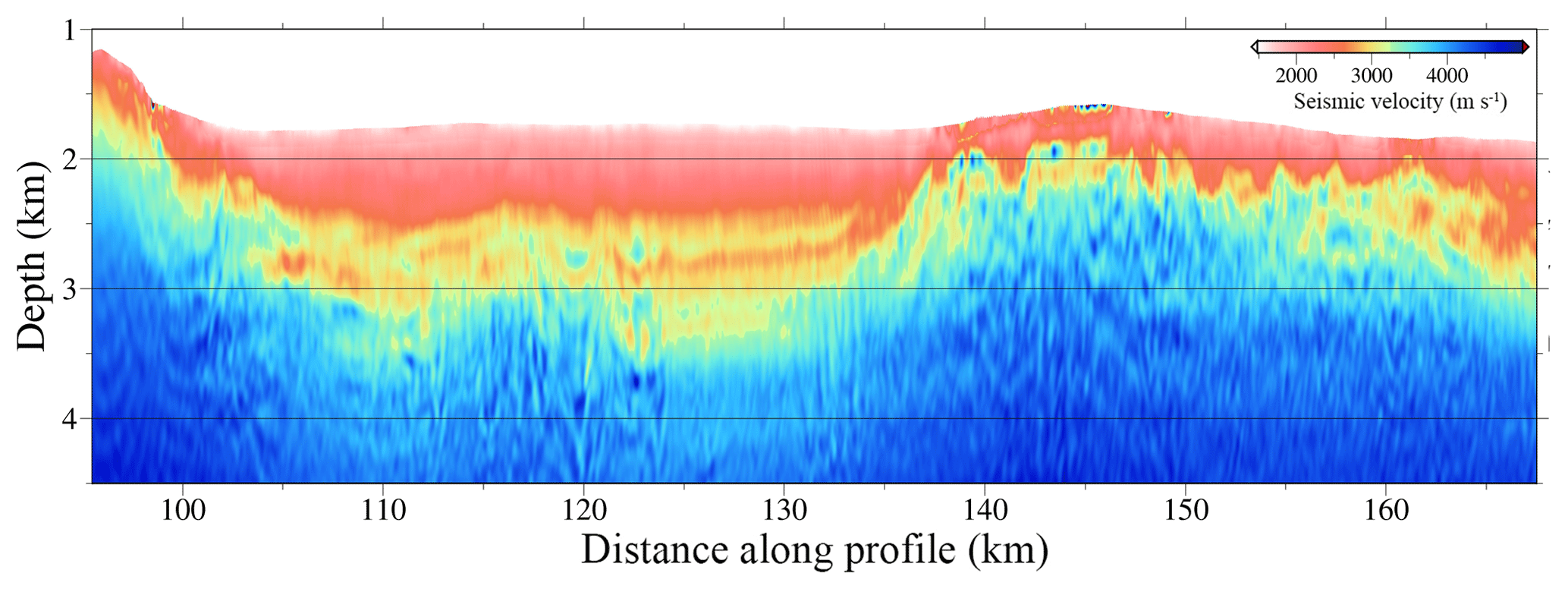
Figure 10 displays the final FWI velocity model. This model has higher resolution than the TTT one (Fig. 7d), showing velocity contrasts of intermediate and short wavelength and a number of geologically meaningful structures that cannot be identified in the TTT model. The improvement due to the higher inverted frequencies is clearer in the shallow part of the model. The velocity contour of ∼3.25 km s⁻¹, which corresponds to the sediment–basement boundary, is better focused and detailed highs and lows are recovered. Thus, in the right-hand side of the profile the velocity variations reproduce the TOB geometry accurately. Dipping low-velocity features are shown with high resolution. The velocity differences between these anomalies and the surrounding media are 0.5–1.0 km s⁻¹ at ∼2.25 km of depth between 137 and 165 km along the profile. The sedimentary package shows velocities from ∼1.7 km s⁻¹ near the seafloor increasing to ∼3.0 km s⁻¹ just above the basement. The blue colour found in the deeper parts of the model corresponds to high velocities of more consolidated rocks. However, there are areas where the high velocities are shallower than in others, due to the action of normal faults, as in the left edge of the model.

A basin from 95 to 137 km distance is displayed between two sloping faults. In addition, a 200–300 m thick, ∼3 km s⁻¹ high-velocity layer ∼25 km long embedded within the sedimentary package is shown up to a volcano-like structure at ∼2.6 km depth. The key point is that all these features have been imaged with a streamer of only 6 km thanks to the workflow followed here.

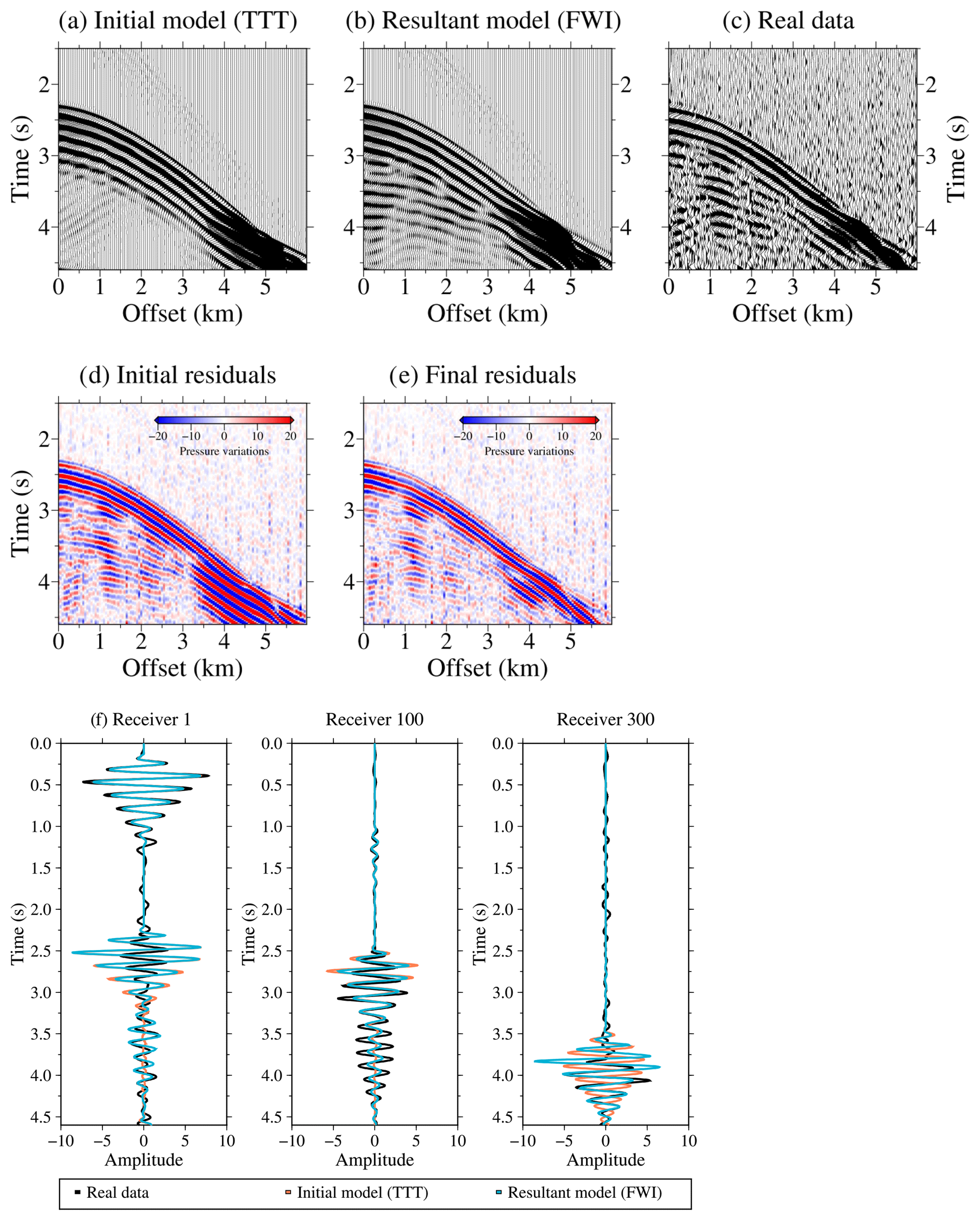
Figure 11 Streamer synthetic seismograms, which are computed using the initial (a) and resultant (b) velocity models presented in Figs. 7d and 10 and the FD solver of the FWI algorithm, together with the real data (c). Only every fourth trace at 50 m is plotted. The location of the streamer is at a distance of ∼101 to 107 km along the profile. Initial (d) and final (e) residuals are displayed for a better comparison of the results, as well as (f) initial (orange; cf. a), resultant (blue; cf. b), and real (black; cf. c) seismic traces for receivers 1, 100, and 300.

To show the model improvement in the data domain, in Fig. 11 we compare a recorded shot gather (Fig. 11c) and a synthetic one generated with the FD solver (Dagnino et al., 2014) using the initial TTT (Fig. 11a) and final FWI (Fig. 11b) velocity models. In contrast with the synthetic data generated with the TTT velocity model (Fig. 11a), the shot gather generated with the FWI velocity model (Fig. 11b) presents some near-vertical reflections. Thus, the seismogram simulated with the final model shows a larger number of seismic events compared to the initial one, which only recovered the first arrival phases and the TOB reflection from the TTT. The data-driven preconditioning of the FWI strategy targeted the energy corresponding to the near-vertical reflections. Therefore, in that region final residuals (Fig. 11e) are smaller than initial ones (Fig. 11d) but are larger around the seafloor reflection. Again, in Fig. 11f aside from wave amplitudes, the main difference between the data generated with the TTT model (orange line) and the target (black line) seismogram is the presence of reflected waves. We observe a better fit between the final (blue line) and real data set (black line), except for the effects that are not modelled, such as 3-D diffractions or the arrivals not included in the data-based preconditioning.

Figure 12 Misfit decrease plotted on a log axis along the iterations. Panel (a) corresponds to the misfit reduction of the seismic information contained in the first multi-scaling step (low-pass filter of 6 Hz), panel (b) to that for an intermediate step (low-pass filter of 11 Hz), and panel (c) to that for the final frequency band (inverted; low-pass filter of 16 Hz).

The misfit reduction for three steps of the multi-scale strategy is shown in Fig. 12. Normalized least-squared misfit is reduced after the whole inversion, and the final residual tends to zero typically after five iterations.

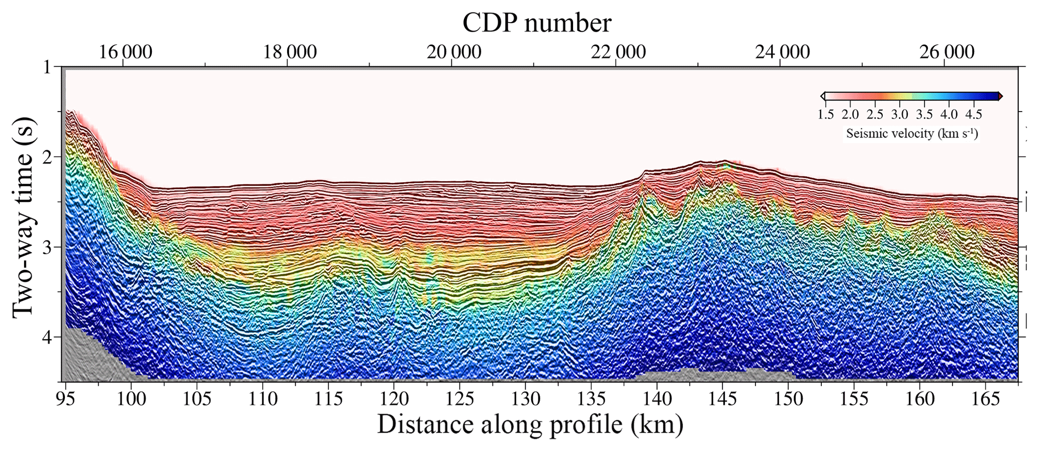
Figure 13 Two-way time-transformed V_P model obtained after the modelling sequence proposed in this paper (joint DC refraction and streamer reflection TTT–FWI) is shown superimposed on the time-migrated MCS image.

As in the case of the TTT model, we have converted the FWI V_P model to two-way time and we have superimposed it to the TMI (Fig. 13). Velocity contrasts present a remarkable match with the reflectors of high amplitude of the TMI. The geometry of the TOB interface reflector, for example, is recovered with great detail. Here, velocity differences are of short wavelength, so many of the details that were previously not displayed can now be properly identified (Fig. 15a).

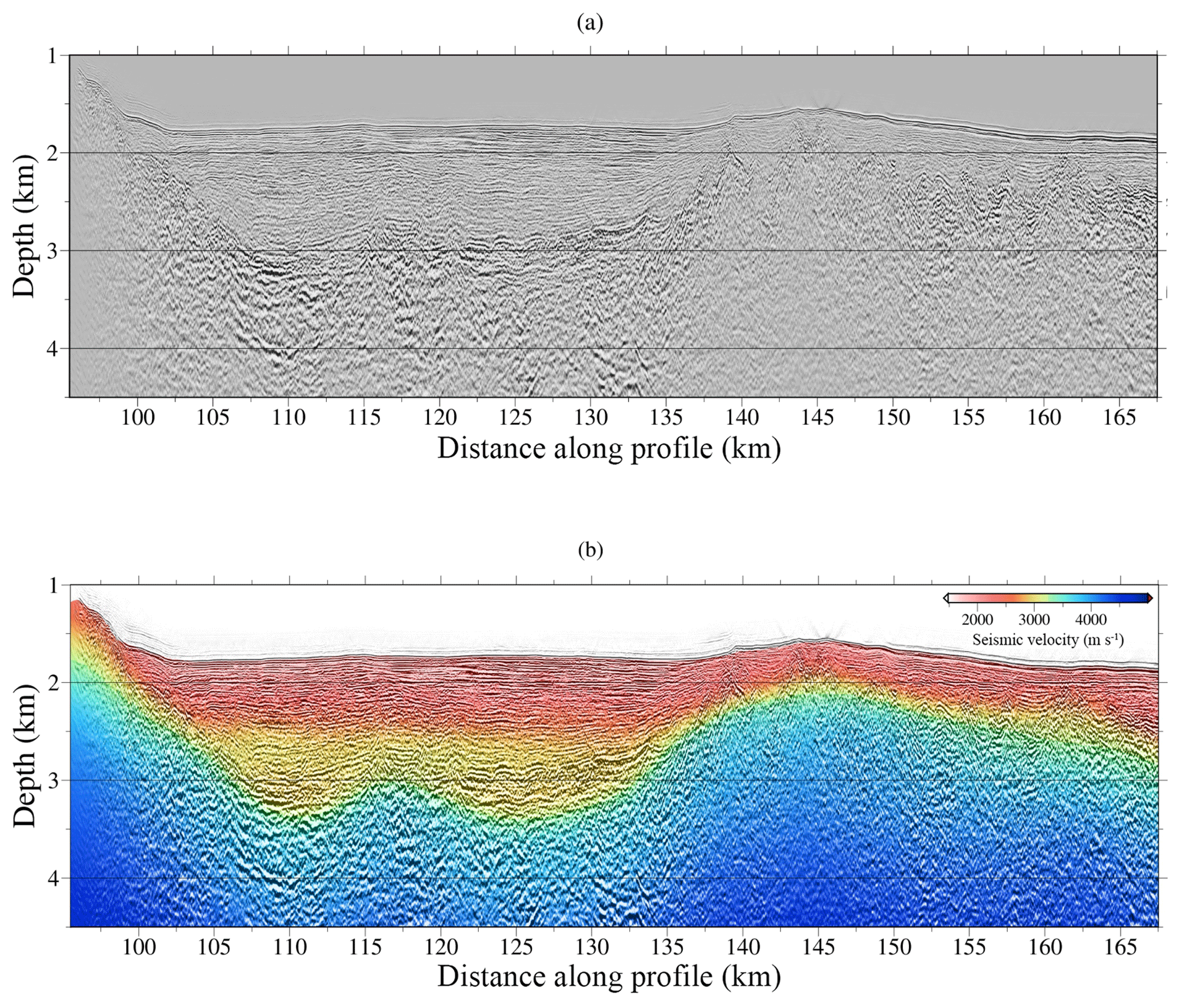
Figure 14 (a) Kirchhoff depth migration result based on the velocity model shown in (b), obtained after the joint DC refraction and streamer reflection TTT.

Figure 15 (a) Geological interpretation superimposed onto Fig. 13. (b) Kirchhoff depth migration result based on the velocity model shown in (c) obtained after the modelling sequence proposed in this paper (joint DC refraction and streamer reflection TTT–FWI). Geological interpretation is also superimposed onto (c).

4.4 Pre-stack depth migration results

The seismic data used for the PSDM are not the same as for FWI but data that have been processed to attenuate coherent and incoherent noise. Streamer field data were processed using a Wiener filter and a surface-consistent deconvolution to increase the vertical resolution attenuating the ringing of the source. Data were sorted in the CDP (common depth point) domain. An amplitude balance (quality factor of 100) was applied to recover the energy lost by geometrical spreading.

We interpolate the FWI result to a 3.125 m grid interval in the horizontal and 3 m in the vertical for the ray tracing. The receivers were spaced at 12.5 m, so the horizontal midpoint distance was 6.25 m for the migration. First, we perform a 2-D Kirchhoff depth migration using the processed data set and the TTT velocity model (Fig. 14a). The same PSDM image is also shown in Fig. 14b superimposed with the TTT velocity model, providing additional information on the rock properties. The resolution of the velocity models obtained through TTT is similar to the typical velocity models built for PSDM, although the latter are based fundamentally on reflections. Thus, the PSDM result shown in Fig. 14 should be comparable to the one that would be obtained with conventional velocity analysis and PSDM. Although the main features are imaged, i.e. the basin geometry, some structures and interfaces are not as well defined as when the PSDM is performed using a high-resolution V_P model, as is shown below.

Finally, we repeat the PSDM but using the final FWI V_P model instead, obtained after the processing–modelling sequence proposed in this work (Fig. 15b and c). An accurate image of the real structure of the shallow subsurface is displayed directly at depth in Fig. 15b. The sediment layer is thicker on the left side of the profile (∼1.5 km), where we find the basin, than on the right (∼0.5 km), where the basement gets shallower. As can be seen in both the FWI velocity model as well as the PSDM image, the basement is severely folded and cut by clear fault structures along the whole profile. The strong lateral velocity changes produced by the faults have caused some migration smiles at the TOB. The deepest part and edges of the profile where FWI and TTT have the largest uncertainties have likewise the largest uncertainty in the PSDM result. On the whole, the vertical section in Fig. 15b shows the correct geometry of the structures at depth with a high resolution, clearer than in Fig. 14 when a TTT model was used. As an example, the depth and location of the TOB boundary is now comparatively more precise.

A good fit is obtained between the shape of the geological features and the isovelocity contours in Fig. 15c. The volcano-like structure and dipping faults, coincide with well-defined velocity anomalies. Furthermore, a high-velocity layer, which was not visible with TTT in Fig. 14b, is also clearly imaged within the sediment package. The combined interpretation helps us to better define the geological structures and to obtain a proper characterization of the nature of the features.

5 Discussion

Information on the structure and properties of the subsurface in the Alboran margin is retrieved by applying a combination of TTT and FWI, particularly the V_P of the sedimentary basin and the geometry of the TOB discontinuity. The area has a heterogeneous vertical and horizontal velocity gradient, with a V_P distribution showing velocity contrasts delineating boundaries of a geologically complex area.

Using the TTT information alone, a coarse V_P model is obtained from no a priori information. No refractions are observed as first arrivals in the original data, so the shot gather recordings are first re-datumed to the seafloor by wave equation downward continuation. We simulate a virtual acquisition system with both sources and receivers located at the seafloor for the TTT, so that refractions can be tracked as first arrivals from zero offset. These near-offset crustal refractions provide excellent structural detail just in the upper portion of our model. But by improving the velocity detail in the upper region of the model (Fig. 7b), we obtain better resolution of the deeper structure (as shown in the second TTT inversion, Fig. 7d). In our case, some deep regions of the model are fitted only by the TOB reflection. Under these circumstances, the inversion result suffers from velocity–depth ambiguity. Streamer TTT exploits the dense and even spatial distribution of MCS data and is further improved upon by DC, which allows for the inclusion of shallower refractions that were only previously obtainable using either seafloor receivers and sources (Henig, 2013). It is important to notice that these highlighted phases would correspond to ray paths in the upper region of the subseafloor section. Moreover, Fig. 9 validates the TTT model obtained, and thereby the travel-time picks used because of the matching of TWT (two-way time)-converted velocity and TOB models with the TMI.

While some studies use waveform modelling in downward continued data (Qin and Singh, 2018), here only the travel-time information is used for inversion. The wave field during the back-propagation is altered due to several factors. The wave field at the virtual positions obtained is affected by grid dispersion and clearly shows amplitude attenuation. Moreover, the field data used to reconstruct the virtual seismogram are a discrete single-sided recording, and, therefore, part of the signal is missing during the back-propagation, hindering the complete reproduction of the wave field. This justifies using travel-time information from the DC shot gathers instead of the whole waveform.

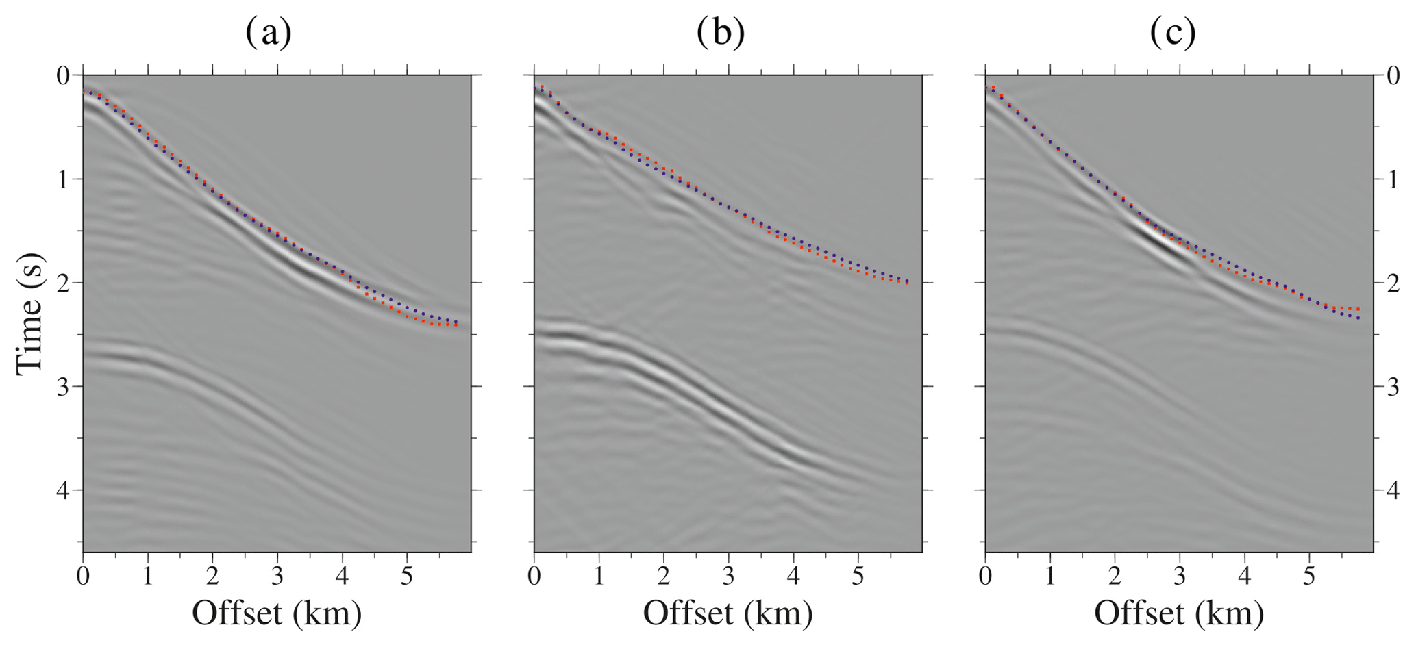
Figure 16 Panels (a)–(c) show synthetic seismic data obtained from the DC of the streamer shots simulated using the final FWI V_P model. From left to right, shot locations are at 171.1, 138.7, and 112.5 km along the profile. First arrivals used as input for the TTT are plotted as blue dots and the ones simulated with the final TTT V_P model as red squares.

The data re-datuming allows recovering and identifying the refracted phases as first arrivals, but not all the energy collapses at its corresponding point, making the first arrival picking even more difficult (see Fig. 6). To check the first arrival travel-time errors introduced by the DC procedure we have reproduced the re-datuming processing but using synthetic shot gathers simulated with the streamer acquisition geometry and the final FWI V_P model (Fig. 10). As is shown in Fig. 16a–c, the first arrivals identified in the real DC shot gathers (blue dots) coincide remarkably well for all offsets with the first arrival travel times of the final TTT V_P model (red squares) and also with the ones in the DC wave fields that are obtained using the synthetic data. The similar results for the first arrivals justify the inclusion of the DC travel times even for large offsets.

The target of applying FWI is to obtain a high-resolution model of the properties of the subsurface. However, due to the non-linear behaviour typical FWI applications use data with low-frequency content or good kinematical starting models from a priori information (e.g. Sirgue and Pratt, 2004; Brossier et al., 2009, 2014; Morgan et al., 2013, 2016). Here, we have implemented and tested a methodological solution (Fig. 1) to overcome this challenge. In our case, the TTT model (Fig. 7d) is essential to perform FWI from data which lack of low frequencies (<6 Hz). As stated in the Introduction, TTT is a very robust technique and commonly used to build good background initial models to FWI (e.g. Shipp and Singh, 2002; Dagnino et al., 2014; Qin and Singh, 2017, 2018). The TTT result is improved here during the FWI by introducing smaller wavenumbers into the V_P model especially from near-vertical reflections (Fig. 11). Despite the higher level of detail, not all the observed signal is matched by the acoustic approach of FWI (Fig. 11). Possible mismatches most likely originate from the presence of noise, elastic (Warner et al., 2013; Marjanovic et al., 2019), anisotropy, or attenuation effects, which were not taken into account. The seafloor reflection is one example of a discontinuity that is hard to fit to the acoustic formulation of the wave propagation.

In both TTT and FWI V_P models, we clearly identify the TOB as an abrupt velocity change. However, the shape of this discontinuity and its velocity contrast differs between the two models in some areas. The FWI result shows sharper boundaries with pronounced dipping contacts at ∼137–167 km along the profile, which are not displayed in the model obtained by TTT. Those dipping contacts, which may represent fault planes in some cases, are of short wavelength and separate zones of abrupt velocity changes that might be associated with lithological variations. This difference becomes more evident at ∼115 km along the profile, where a volcano-like structure is imaged. This feature might be a volcano due to the location of the profile, which crosses an area where there is supposed to be a volcanic arc. Moreover, the geometry of the volcano-like structure and irregular TOB boundary is only clearly imaged at depth when the PSDM is performed with the high-resolution V_P model provided by FWI (compare Figs. 15 and 14). In addition, the high-velocity layer within sediments on top of this structure is only clearly defined in the FWI V_P model (Fig. 10). This layer is likely to be an evaporite layer deposited during the Messinian crisis.

To assess the match of the velocity model to the seismic boundaries obtained with more traditional processing and imaging, the V_P model is converted to two-way time and compared with the TMI. As state above, the two-way time-transformed velocity model has an excellent match with MCS time migration; velocity changes nicely follow major reflectivity contrasts and fault locations (Fig. 13), which further support the quality of the inversion result and workflow.

6 Geological structure

The seismic line was collected to image the structure of the eastern Alboran Basin in a region where basement is interpreted to be made up of magmatic arc rocks (Booth-Rea et al., 2007, 2018; Gómez de la Peña et al., 2018). The time migration and PSDM show a sediment basin with basement highs on either end of the image. The large basement highs in the flank display some indications of extensional faulting and block tilting, particularly in the NE. These faults worked during the formation of the basin and may have some syntectonic sediment tilted in between rotated fault blocks, but the faults were not active during the deposition of most of the sediment cover.

The basement top under the basin and also along the southern ridge displays several small-scale highs with steep flanks and a triangular shape with fairly symmetric flanks that do not support tectonic rotation and may indicate small-scale volcanoes, so that the image supports the basement formation by the interplay between magmatic and extensional processes as expected in a magmatic arc.

The sediment cover displays several units bound by unconformities and cut by small sub-vertical, currently active faults. Based on regional geology, we infer that most of the sediment sequence is possibly Pliocene but the oldest layers may be late Miocene, although no drill hole in the vicinity provides a calibration. The seismic velocity distribution in the basin infill may provide some further clues regarding the age and nature of the sediment. The V_P model of the largest basin shows a gradual increase in velocity with depth to V_P ∼3 km s⁻¹ (change from reddish to orange colour in Fig. 15a, c) that changes abruptly by ∼0.5 km s⁻¹ in a slower-velocity body (change from orange to reddish in Fig. 15a, c). This high- to low-velocity change is marked by a high-amplitude reflection that marks an unconformity – possibly erosional – with the underlying unit. The high velocity is anomalous because clastic material – turbidities in most of the basin – typically increases in V_P with a compaction-driven decrease in porosity. The high-velocity layer may indicate the presence of evaporites from the end of the Messinian period characterized across much of the Mediterranean by a relatively large drop-down of the water level and the deposition of oversaturated deposits. In the deep basin further to the east there are considerably thick salt deposits that can be easily identified in seismic reflection images due to the mobility and formation of diapiric structures (Booth-Rea et al., 2007). Here, in the region of this study there are no known salt deposits, and the presence of Messinian deposits without drilling information is unconstrained. A potential interpretation is that the high-velocity layer represents an anhydrite-rich layer that has relatively high velocities (like salt layers), but it is not as mobile.

7 Conclusions

We show that the proposed workflow, including DC of MCS data to the seafloor, joint refraction, and reflection TTT and FWI, allows obtaining a detailed, geologically meaningful V_P model from a non-optimal data set. Although the streamer length is only 6 km, the water depth is fairly great (∼2 km), and seismic records lack low frequencies (<6 Hz), the inversion converged, successfully providing a detailed velocity model to a depth of 3–4 km. The excellent match between the two-way time-transformed velocity model and the time-migrated MCS image validates the results. The PSDM images together with the V_P model reproduce the structures and properties of the sedimentary layers and the uppermost part of the basement with high resolution directly in the depth domain. Aside from the irregular TOB, a volcano-like structure and steeply dipping anomalies at the flanks of the basin that may correspond to faults are clearly imaged. Moreover, the model allows identifying the location, geometry, thickness, and velocity of a high-velocity layer (possibly evaporites on top of the Messinian unconformity) embedded within sediments. We conclude that the proposed method is valid and can be applied under these circumstances. Applying it to longer streamer data should improve V_P models and allow extending the models to greater depths. Here, we recover all the possible subsurface information from the MCS recordings alone. Future research can be directed to apply this strategy to longer-offset data from wide-angle acquisition geometries to increase the coverage and to better constrain the model properties.