Anisotropic P-wave travel-time tomography implementing Thomsen's weak approximation in TOMO3D

We present the implementation of Thomsen's weak anisotropy approximation for vertical transverse isotropy (VTI) media within TOMO3D, our code for 2-D and 3-D joint refraction and reflection travel-time tomographic inversion. In addition to the inversion of seismic P-wave velocity and reflector depth, the code can now retrieve models of Thomsen's parameters (δ and ε). Here, we test this new implementation following four different strategies on a canonical synthetic experiment in ideal conditions with the purpose of estimating the maximum capabilities and potential weak points of our modeling tool and strategies. First, we study the sensitivity of travel times to the presence of a 25 % anomaly in each of the parameters. Next, we invert for two combinations of parameters (v, δ, ε and v, δ, v^⊥), following two inversion strategies, simultaneous and sequential, and compare the results to study their performance and discuss their advantages and disadvantages. Simultaneous inversion is the preferred strategy and the parameter combination (v, δ, ε) produces the best overall results. The only advantage of the parameter combination (v, δ, v^⊥) is a better recovery of the magnitude of v. In each case, we derive the fourth parameter from the equation relating ε, v^⊥ and v. Recovery of v, ε and v^⊥ is satisfactory, whereas δ proves to be impossible to recover even in the most favorable scenario. However, this does not hinder the recovery of the other parameters, and we show that it is still possible to obtain a rough approximation of the δ distribution in the medium by sampling a reasonable range of homogeneous initial δ models and averaging the final δ models that are satisfactory in terms of data fit.

1 Introduction

An isotropic velocity field is the rare exception in the Earth subsurface. Anisotropy is a multiscale phenomenon, and its causes are diverse. In the crust, it can be produced by the preferred orientation of mineral grains or their crystal axes (Schulte-Pelkum and Mahan, 2014; Almqvist and Mainprice, 2017), the alignment of cracks and fracture networks and the presence of fluids (Crampin, 1981; Maultzsch et al., 2003; Yousef and Angus, 2016), or the bedding of layers much thinner than the wavelength used to explore them (Backus, 1962; Johnston and Christensen, 1995; Sayers, 2005). In the mantle, anisotropy is related to the alignment of olivine crystals due to mantle flow (Nicolas and Christensen, 1987; Montagner et al., 2007), aligned melt inclusions (Holtzman et al., 2003; Kendall et al., 2005), large-scale deformation (Vinnik et al., 1992; Vauchez et al., 2000) and pre-existing lithospheric fabric (Kendall et al., 2006), among others. Anisotropy has proven an informative physical property in the understanding of the Earth's interior (Ismaïl and Mainprice, 1998; Long and Becker, 2010), most particularly in continental rifts (Eilon et al., 2016), mid-ocean ridges (Dunn et al., 2001) and subduction zones (Long and Silver, 2008).

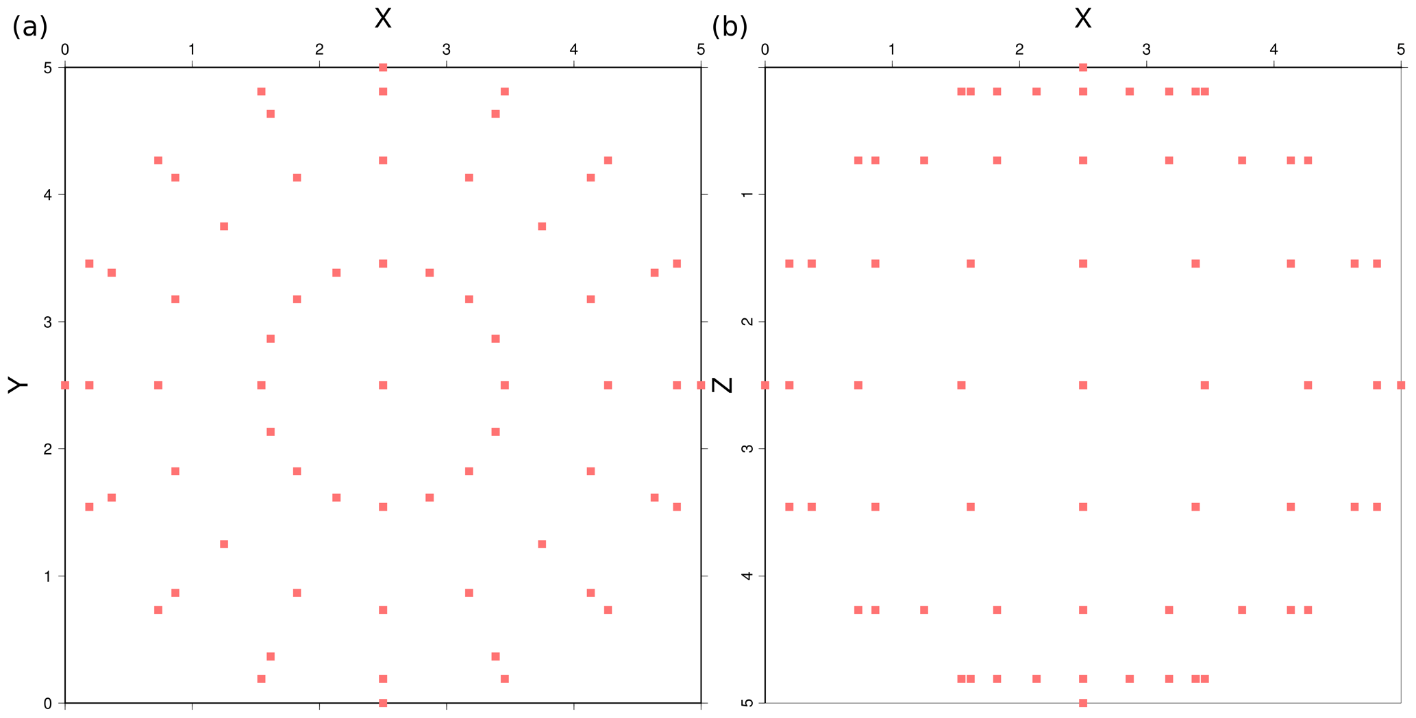
Figure 1 (a) Horizontal and (b) vertical views of the acquisition geometry for the inversion tests. Overall, 114 sources and 114 receivers (red boxes) are located at 2.5 km from the center of the model at the locus defined by the surface of the sphere inscribed in the cube and placed at the crossing points of 16 meridians with 7 parallels and at each pole. Thus, in the inversion tests, we used 12 882 travel times from 114 sources, each recorded at 113 receivers; i.e., all receivers record all sources, except for the one coinciding in location. The acquisition geometry for the accuracy and sensitivity tests is similar, only in this case for sources and receivers at the crossing points of 32 meridians and 15 parallels, plus one of each at the two poles, and using just 482 travel times from diametrically opposed source–receiver pairs arranged; i.e., each receiver exclusively records the first-arrival travel time from its paired source.

The theory of anisotropic wave propagation has been described in several publications (Kraut, 1963; Babuska and Cara, 1991). Numerous formulations of varying complexity have been proposed to approximate anisotropy depending on its magnitude and the symmetry conditions of the medium (Nye, 1957). Overall, 21 elastic stiffness parameters define the most general anisotropic medium with the lowest symmetry conditions, whereas for the highest symmetry not equivalent to isotropy, only five parameters are needed (Almqvist and Mainprice, 2017). Regarding the strength of anisotropy, in view of the overall success of isotropic methods in studying the Earth's subsurface, and of the experimental evidence and sample measurements available, it is admitted that the anisotropy is generally weak (Thomsen, 1986). Specifically, anisotropy is considered weak when Thomsen's parameters are much smaller than 1, i.e., for a ∼20 % or smaller velocity variation with angle. Precisely Thomsen (1986) presented the formulation for the transverse isotropy symmetry on weakly anisotropic media, which is the reference that we follow in this work. Thomsen's parameters are by far the most common and convenient combinations of stiffness tensor elements used in seismic anisotropy modeling (Tsvankin, 1996; Thomsen and Anderson, 2015). Applications of simpler approximations exist, as is the case of elliptical symmetry (Song et al., 1998; Giroux and Gloaguen, 2012), as well as others that assume the most general anisotropic model (Zhou and Greenhalgh, 2008).

The objectives of this work are (1) presenting the anisotropic version of TOMO3D (Meléndez et al., 2015b) for the study of vertical transverse isotropy (VTI) weakly anisotropic media in terms of Thomsen's parameters (δ and ε) using P-wave arrival times and (2) comparing several parameterizations and inversion strategies under optimal and equal conditions for all parameters with the purpose of defining an upper limit of the code's capabilities, an ideal but generalizable estimation of the code's performance, as well as highlighting its potential weaknesses. Moreover, the development of this code is motivated by the need to combine wide-angle and near-vertical travel-time picks in field data applications, as we plan to do with the trench-parallel 2-D profile in Sallarès et al. (2013), which is affected by a ∼15 % anisotropy judging from the mismatch in the interplate boundary locations obtained separately from near-vertical and wide-angle data. The P-wave velocity, δ and ε models obtained from the modeling of field data would be useful and geologically informative by themselves, but they would also serve as initial models in anisotropic full waveform inversion (FWI).

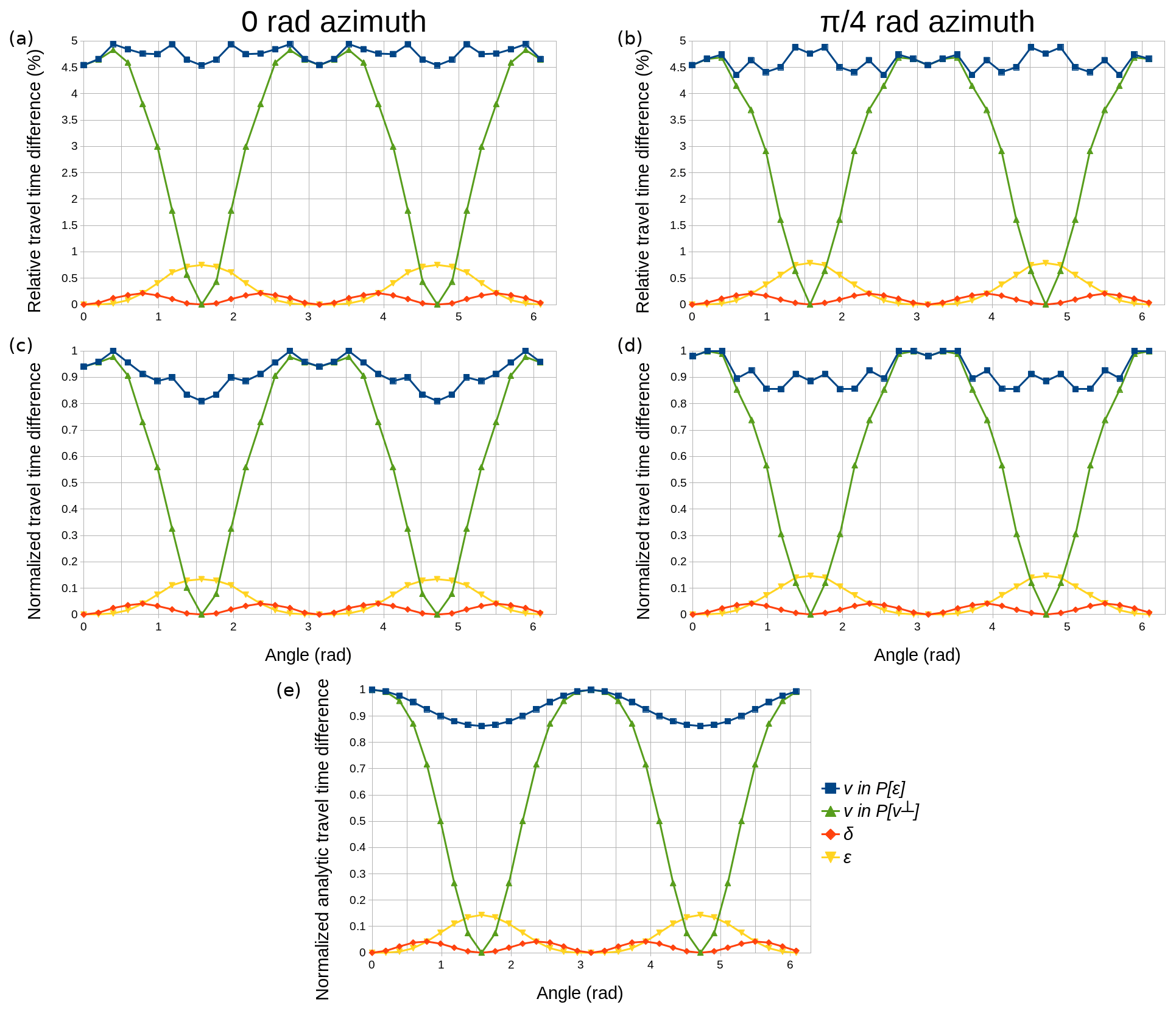
Figure 2 Sensitivities for the meridians at azimuths 0 rad (a, c) and π∕4 rad (b, d) as a function of the polar angle (origin in the downward vertical axis). (a, b) Synthetic relative sensitivities in percentage, (c, d) synthetic normalized sensitivities and (e) normalized analytic sensitivities. Sensitivity values displayed correspond to all source–receiver pairs along the selected meridians of the acquisition configuration.

In the following section, we describe the anisotropy formulation and the modifications implemented on our 3-D joint refraction and reflection travel-time tomography code TOMO3D to incorporate the inversion of Thomsen's parameters. Next, in Sect. 3, we present the synthetic tests performed and their results, including accuracy and sensitivity analyses and synthetic inversions. In Sect. 4, these results are discussed and interpreted in terms of the ability of the code to retrieve both the velocity field and Thomsen's anisotropy parameters. Finally, in the last section, we summarize the main conclusions of this work.

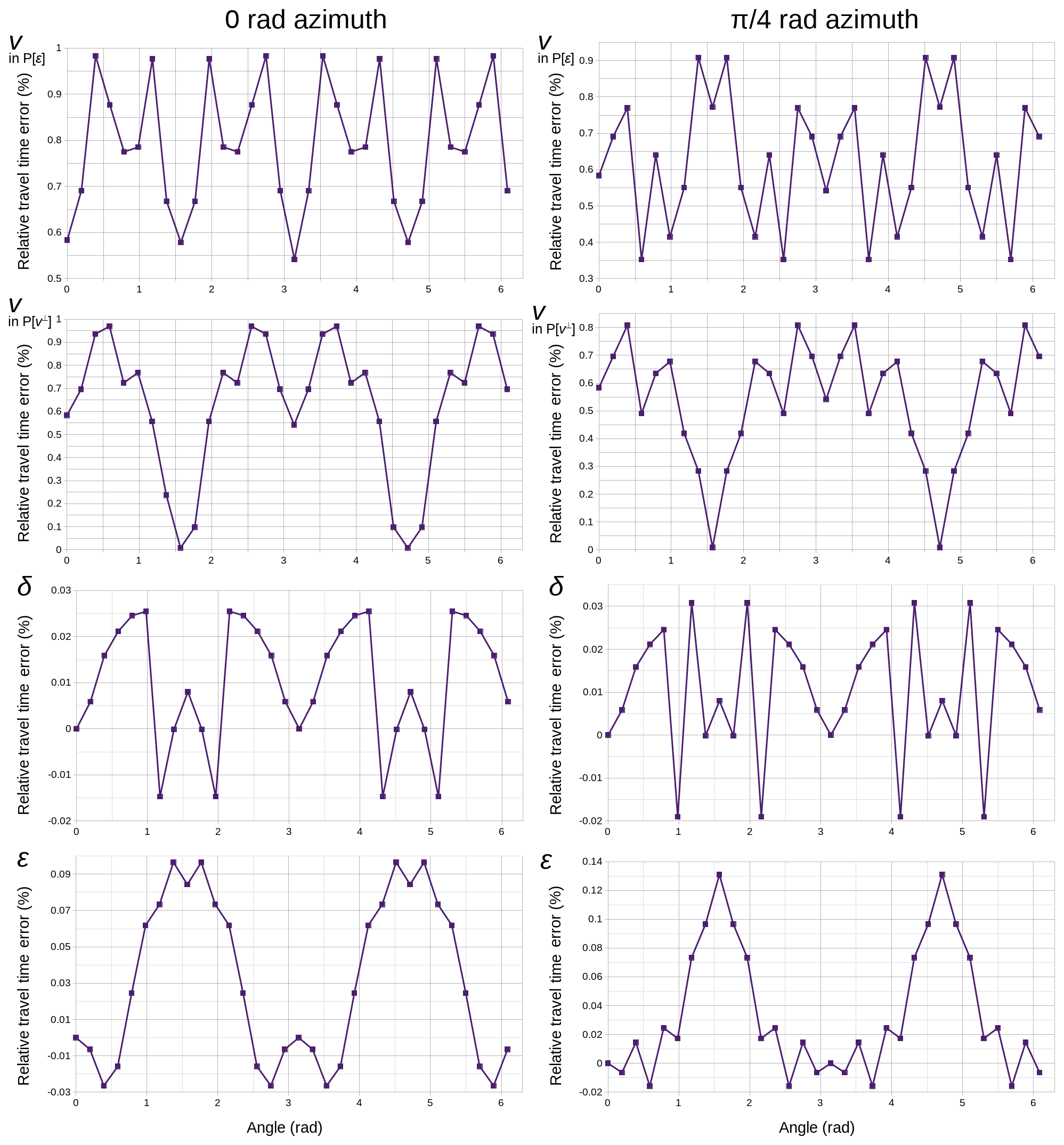
Figure 3 For both selected meridians, 0 rad and π∕4 rad azimuths, relative travel-time errors in percentage with respect to the analytic value for each of the four simulations used in the sensitivity analysis. Polar angle origin is in the downward vertical axis. Mean values and deviations are shown in Table 2.

2 Modeling anisotropy

The first part of this section is a general overview of the treatment of anisotropy within the field of seismic inversion, while the second one describes the implementation of Thomsen's weak VTI anisotropy formulation in the 3-D joint refraction and reflection travel-time tomography code TOMO3D.

2.1 Anisotropy in seismic inversion methods

Anisotropy was first incorporated to seismic inversion methods in travel-time tomography with the development of the linearized perturbation theory (Cervený, 1982; Cervený and Jech, 1982; Jech and Psencik, 1989). Previously, the approach to deal with anisotropy was to approximately remove its estimated effect to then apply an isotropic method (e.g., McCann et al., 1989). Linearized perturbation theory was first implemented in anisotropic travel-time tomography by Chapman and Pratt (1992) and Pratt and Chapman (1992), assuming the weak anisotropy approximation, which allowed them to use isotropic ray tracing and approximate anisotropy effects as being caused by small perturbations of the isotropic system. The initial development of anisotropic ray tracing is attributed to Cervený (1972). Methods for anisotropic ray tracing and travel-time computation depend on the symmetry assumptions made regarding the medium. The most common of those is rotational symmetry around a vertical pole. This formulation is known as VTI and also polar anisotropy (e.g., Rüger and Alkhalifah, 1996; Alkhalifah, 2002), and it is the simplest geologically applicable case: it reproduces the symmetry exhibited by minerals in sedimentary rocks and that produced by parallel cracks or fine layering. Furthermore, it significantly simplifies the mathematical formulae since anisotropy is defined by only five parameters, which contributes to a greater computational efficiency. The generalization of VTI to a tilted symmetry axis is the so-called tilted transverse isotropy (TTI). Some authors argue that it is not possible to distinguish TTI from VTI in real experimental cases without a priori information (Bakulin et al., 2009). Assuming the most general anisotropic media has also become rather usual, in particular with the improvement of computational resources, allowing for a more detailed and complex reconstruction of the subsurface physical properties (e.g., Zhou and Greenhalgh, 2005), although successful field data applications are yet to be achieved to the best of our knowledge. Regarding the inversion process, the main difficulty arises from the trade-off between velocity heterogeneity and anisotropy (e.g., Bezada et al., 2014). To the best of our knowledge, Stewart (1988) was the first to propose an inversion algorithm, specifically for the recovery of Thomsen's parameters in a weakly anisotropic VTI medium. Other authors have produced inversion algorithms for different formulations such as azimuthal anisotropy (e.g., Eberhart-Phillips and Henderson, 2004; Dunn et al., 2005) or a 3-D TTI medium (e.g., Zhou and Greenhalgh, 2008). Concerning FWI, anisotropy in active data is typically modeled following Thomsen's parameters and the VTI and/or TTI approximation for the medium. The first anisotropic wave propagators appeared during the 1980s and 1990s (e.g., Helbig, 1983; Alkhalifah, 1998) and new improvements on this matter continue today (e.g., Fowler et al., 2010; Duveneck and Bakker, 2011). When performing anisotropic FWI, both 2-D and 3-D, some authors choose to invert only for the velocity field, fixing the initial anisotropy models throughout the inversion because it simplifies the process (e.g., Prieux et al., 2011; Warner et al., 2013). However, other works have explored the feasibility of multiparameter inversions, that is, using different combinations of velocity and anisotropy parameters and of inversion strategies (e.g., Gholami et al., 2013a, b; Alkhalifah and Plessix, 2014).

2.2 Anisotropy in TOMO3D: Thomsen's weak VTI anisotropy formulation

We adapted TOMO3D (Meléndez et al., 2015b) to perform anisotropic ray tracing and travel-time calculations, as well as inversion of Thomsen's parameters for P-wave data (Meléndez et al., 2015a). In TOMO3D, the forward problem solver is parallelized to simultaneously trace rays for multiple sources and receivers, and it uses an hybrid ray-tracing algorithm that combines the graph or shortest path method (Moser, 1991) and the bending refinement method (Moser et al., 1992). The inverse problem is solved sequentially using the LSQR algorithm (Paige and Saunders, 1982). Velocity models are discretized as 3-D orthogonal and vertically sheared grids that can account for topography and/or bathymetry. Velocity values are assigned to the grid nodes, and the velocity field is built by trilinear interpolation within each cell. Apart from first-arrival travel times, the code allows for the inversion of reflection travel times to obtain the geometry of major geological boundaries associated with impedance contrasts that produce strong seismic energy reflections in the data recordings. Such reflecting interfaces are modeled as 2-D grids independent of the velocity grid. The code is also prepared to extract information from the water-layer multiple of refracted and reflected seismic phases (Meléndez et al., 2014). A detailed description of the code can be found in Meléndez (2014).

Our anisotropy formulation is based on Thomsen (1986) and specifically in the following weakly anisotropic velocity equation for the P-wave velocity:

$$\begin{array}{}\text{(1)}& v^{\mathrm{a}}\left(v,\mathit{\delta },\mathit{\epsilon },\mathit{\theta }\right)=v\cdot \left(\mathrm{1}+\mathit{\delta }\cdot {\sin }^{\mathrm{2}}\left(\mathit{\theta }\right)\cdot {\cos }^{\mathrm{2}}\left(\mathit{\theta }\right)+\mathit{\epsilon }\cdot {\sin }^{\mathrm{4}}\left(\mathit{\theta }\right)\right),\end{array}$$

where v^a is the anisotropic velocity, v is the velocity along the symmetry axis (α₀ in Thomsen, 1986), θ is the angle with respect to the symmetry axis, and δ and ε are Thomsen's parameters controlling the anisotropic P-wave propagation. Studying the cases of θ=0 and $\mathit{\theta }=\mathit{\pi }/\mathrm{2}$, the meaning of ε becomes clear: it is the relative difference between the velocities along and across the symmetry axis that we refer to as parallel and perpendicular velocities, respectively.

$$\begin{array}{}\text{(2)}& \begin{array}{rl}& v^{\mathrm{a}}\left(v,\mathit{\theta }=\mathrm{0}\right)=v\\ & v^{\mathrm{a}}\left(v,\mathit{\theta }={\displaystyle \frac{\mathit{\pi }}{\mathrm{2}}}\right)=v\cdot \left(\mathrm{1}+\mathit{\epsilon }\right)\equiv v^{\perp }\\ & \mathit{\epsilon }=(v^{\perp }-v)/v\end{array}\end{array}$$

According to Thomsen (1986), the meaning of δ is far from intuitive, but the author states that it is associated with the near-vertical anisotropic response and shows that it relates v and the normal move-out velocity (V_NMO). V_NMO models are a byproduct of multichannel seismic reflection data processing, a mathematical construct that involves the assumptions of a stratified media with constant velocity layers and of small spread, i.e., near-vertical propagation. It does not seem wise to try estimating it by other means, less so if the data and modeling used do not necessarily fulfill the assumptions for the normal move-out correction that define V_NMO. Moreover, we want to combine travel times from as many types of seismic data sets as possible, notably from multichannel reflection (near-vertical propagation) and wide-angle (subhorizontal propagation) experiments, in order to have the best polar coverage, and with that, the best recovery of v and ε (or v^⊥). Thus, we do not consider V_NMO to be a useful parameter in describing the general anisotropic VTI media for our modeling method, and we did not implement parameterizations (v,V_NMO,ε and v,$V_{\mathrm{NMO}},v^{\perp }$). We do think, however, that V_NMO models can help in the building of initial δ models, just as the comparison between near-vertical propagation and subhorizontal data can provide an initial estimation of ε. In conclusion, we only considered Eq. (2), and we implemented two parameterizations of the medium: (v, δ, ε) and (v, δ, v^⊥). From here on, for simplicity, we will refer to them as P[ε] and P[v^⊥], respectively.

The linearized inverse problem matrix equation including anisotropy parameters for a refraction-only case is as follows:

$$\begin{array}{}\text{(3)}& \left(\begin{array}{c}\mathbf{\Delta }{t}^{\mathrm{0}}\\ \mathrm{0}\\ \mathrm{0}\\ \mathrm{0}\\ \mathrm{0}\\ \mathrm{0}\\ \mathrm{0}\\ \mathrm{0}\\ \mathrm{0}\\ \mathrm{0}\\ \mathrm{0}\\ \mathrm{0}\\ \mathrm{0}\end{array}\right)=\left(\begin{array}{ccc}{\mathbf{G}}^{u\mathrm{0}}& {\mathbf{G}}^{\mathit{\delta }\mathrm{0}}& {\mathbf{G}}^{\mathit{\epsilon }\mathrm{0}}\\ {\mathit{\lambda }}_u{\mathbf{L}}^{uX}& \mathrm{0}& \mathrm{0}\\ {\mathit{\lambda }}_u{\mathbf{L}}^{uY}& \mathrm{0}& \mathrm{0}\\ {\mathit{\lambda }}_u{\mathbf{L}}^{uZ}& \mathrm{0}& \mathrm{0}\\ \mathrm{0}& {\mathit{\lambda }}_{\mathit{\delta }}{\mathbf{L}}^{\mathit{\delta }X}& \mathrm{0}\\ \mathrm{0}& {\mathit{\lambda }}_{\mathit{\delta }}{\mathbf{L}}^{\mathit{\delta }Y}& \mathrm{0}\\ \mathrm{0}& {\mathit{\lambda }}_{\mathit{\delta }}{\mathbf{L}}^{\mathit{\delta }Z}& \mathrm{0}\\ \mathrm{0}& \mathrm{0}& {\mathit{\lambda }}_{\mathit{\epsilon }}{\mathbf{L}}^{\mathit{\epsilon }X}\\ \mathrm{0}& \mathrm{0}& {\mathit{\lambda }}_{\mathit{\epsilon }}{\mathbf{L}}^{\mathit{\epsilon }Y}\\ \mathrm{0}& \mathrm{0}& {\mathit{\lambda }}_{\mathit{\epsilon }}{\mathbf{L}}^{\mathit{\epsilon }Z}\\ {\mathit{\alpha }}_u{\mathbf{D}}^u& \mathrm{0}& \mathrm{0}\\ \mathrm{0}& {\mathit{\alpha }}_{\mathit{\delta }}{\mathbf{D}}^{\mathit{\delta }}& \mathrm{0}\\ \mathrm{0}& \mathrm{0}& {\mathit{\alpha }}_{\mathit{\epsilon }}{\mathbf{D}}^{\mathit{\epsilon }}\end{array}\right)\left(\begin{array}{c}\mathbf{\Delta }u\\ \mathbf{\Delta }\mathit{\delta }\\ \mathbf{\Delta }\mathit{\epsilon }\end{array}\right).\end{array}$$

Smoothing (L) and damping (D) constraints for δ and ε parameters follow the same formulation described in Meléndez (2014) for velocity parameters. The kernels (G) have been modified to account for anisotropy. The linearized and discretized equation that relates the travel-time residual of the nth refracted pick to changes in the model parameters is written as

$$\begin{array}{}\text{(4)}& \begin{array}{rl}\mathrm{\Delta }{t}_n^{\mathrm{0}}& ={\sum }_i^I{\sum }_{m=\mathrm{1}}^{\mathrm{8}}{r}_m^u\cdot {\displaystyle \frac{\partial t}{\partial u^{\mathrm{a}}}}\cdot {\displaystyle \frac{\partial u^{\mathrm{a}}}{\partial u}}\cdot \mathrm{\Delta }{u}_i\\ & +{\sum }_j^J{\sum }_{m=\mathrm{1}}^{\mathrm{8}}{r}_m^{\mathit{\delta }}\cdot {\displaystyle \frac{\partial t}{\partial u^{\mathrm{a}}}}\cdot {\displaystyle \frac{\partial u^{\mathrm{a}}}{\partial \mathit{\delta }}}\cdot \mathrm{\Delta }{\mathit{\delta }}_j\\ & +{\sum }_k^K{\sum }_{m=\mathrm{1}}^{\mathrm{8}}{r}_m^{\mathit{\epsilon }}\cdot {\displaystyle \frac{\partial t}{\partial u^{\mathrm{a}}}}\cdot {\displaystyle \frac{\partial u^{\mathrm{a}}}{\partial \mathit{\epsilon }}}\cdot \mathrm{\Delta }{\mathit{\epsilon }}_k\end{array}.\end{array}$$

In each of the three terms, the first summation corresponds to the model cells that are illuminated by the nth ray path. A cell is considered illuminated if it contains a ray path segment. The second summation is over the eight nodes of each of those cells. In the third term, ε is replaced by v^⊥ when using this alternative parameterization. $\mathrm{\Delta }{t}_n^{\mathrm{0}}$ is the travel-time residual for the nth refracted pick, u^a=1/v^a is the anisotropic slowness, $u=\mathrm{1}/v$ is the along-axis slowness, Δu_i, Δδ_j and Δε_k (or $\mathrm{\Delta }{v}_k^{\perp }$) are the parameter perturbations for each illuminated cell in their respective grids, and the r_m factors are the weights that distribute these perturbations among the eight nodes of each illuminated cell according to the trilinear interpolation used to define the four fields (u, δ, ε and v^⊥).

In order to build the kernel matrices, we need to compute two partial derivatives for each model parameter. The first-order partial derivative of travel time with respect to the anisotropic slowness is the ray path segment s_i within each cell that is covered in a given travel time at a given slowness:

$$\begin{array}{}\text{(5)}& {\displaystyle }t={\sum }_{i=\mathrm{1}}^N{u}_i^{\mathrm{a}}\cdot s_i\text{(6)}& {\displaystyle \frac{\partial t}{\partial u_i^{\mathrm{a}}}}=s_i.\end{array}$$

From Eq. (1), the first-order partial derivatives of the anisotropic slowness with respect to the model parameters (u, δ, ε and v^⊥) are as follows:

$$\begin{array}{}\text{(7)}& {\displaystyle \frac{\partial u^{\mathrm{a}}}{\partial u}}={\displaystyle \frac{\mathrm{1}}{\mathrm{1}+\mathit{\delta }\cdot {\sin }^{\mathrm{2}}\left(\mathit{\theta }\right)\cdot {\cos }^{\mathrm{2}}\left(\mathit{\theta }\right)+\mathit{\epsilon }\cdot {\sin }^{\mathrm{4}}\left(\mathit{\theta }\right)}}\text{(8)}& {\displaystyle \frac{\partial u^{\mathrm{a}}}{\partial \mathit{\delta }}}={\displaystyle \frac{-u\cdot {\sin }^{\mathrm{2}}\left(\mathit{\theta }\right)\cdot {\cos }^{\mathrm{2}}\left(\mathit{\theta }\right)}{{\left(\mathrm{1}+\mathit{\delta }\cdot {\sin }^{\mathrm{2}}\left(\mathit{\theta }\right)\cdot {\cos }^{\mathrm{2}}\left(\mathit{\theta }\right)+\mathit{\epsilon }\cdot {\sin }^{\mathrm{4}}\left(\mathit{\theta }\right)\right)}^{\mathrm{2}}}}\text{(9)}& {\displaystyle \frac{\partial u^{\mathrm{a}}}{\partial \mathit{\epsilon }}}={\displaystyle \frac{-u\cdot {\sin }^{\mathrm{4}}\left(\mathit{\theta }\right)}{{\left(\mathrm{1}+\mathit{\delta }\cdot {\sin }^{\mathrm{2}}\left(\mathit{\theta }\right)\cdot {\cos }^{\mathrm{2}}\left(\mathit{\theta }\right)+\mathit{\epsilon }\cdot {\sin }^{\mathrm{4}}\left(\mathit{\theta }\right)\right)}^{\mathrm{2}}}}\text{(10)}& {\displaystyle \frac{\partial u^{\mathrm{a}}}{\partial v^{\perp }}}={\displaystyle \frac{-{\left(u\right)}^{\mathrm{2}}\cdot {\sin }^{\mathrm{4}}\left(\mathit{\theta }\right)}{{\left(\mathrm{1}+\mathit{\delta }\cdot {\sin }^{\mathrm{2}}\left(\mathit{\theta }\right)\cdot {\cos }^{\mathrm{2}}\left(\mathit{\theta }\right)+\mathit{\epsilon }\cdot {\sin }^{\mathrm{4}}\left(\mathit{\theta }\right)\right)}^{\mathrm{2}}}}.\end{array}$$

3 Synthetic tests

We have performed a number of tests using canonical synthetic models made of an anomaly centered in a uniform background with two main objectives: (1) checking that the newly implemented anisotropic travel-time tomography method works properly and (2) providing a quantitative measure of the potential recovery of anisotropy based on P-wave travel times alone. All data and files used for these synthetic tests are available at the digital CSIC repository (Meléndez et al., 2019). First, we run a sensitivity test to assess the effect that a variation in each model parameter has in the synthetic travel times, and we calibrated the code by comparing the synthetic data that it generates to analytically calculated data. Next, we performed a number of synthetic inversion tests considering both possible parameterizations and inversion strategies. These tests are conducted under ideal and equal conditions for all parameters with the purpose of obtaining an upper limit but widely applicable estimation of the code's performance and detecting any potential weak points.

The models in all these tests are cubes with 5 km long edges. The background model of all four parameters is set to a constant value; i.e., v, δ, ε and v^⊥ background models are homogeneous. Note that the z-axis positive direction points downwards. Grid spacing is 0.125 km for the four parameters in all three dimensions, so that differences in model discretization do not influence the test results. The volume of the anomaly is determined by the 3σ region of a 3-D Gaussian function centered in the cube setting 3σ=0.5 km. The values of v, δ, ε and v^⊥ within this volume are homogeneously increased, resulting in a discretized representation of a spherical anomalous body.

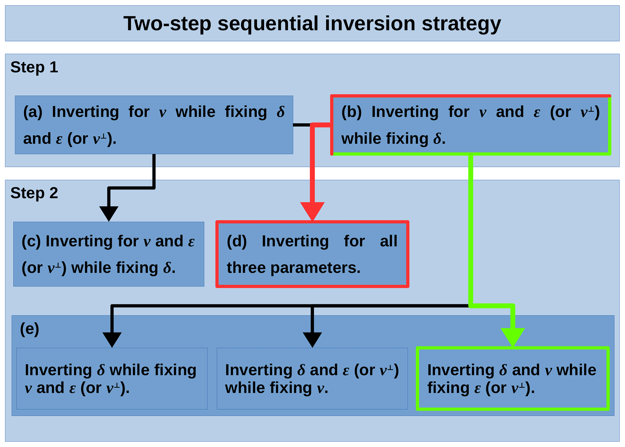
Figure 4 Flowchart describing the two steps for all the sequential inversion options tested. The best options for the sequential inversion strategy in P[ε] (Fig. 7) and in P[v^⊥] (Fig. 8) are marked in green and red, respectively.

3.1 Sensitivity

We define the sensitivity of a parameter as the difference between the first-arrival travel times with and without the anomaly in that parameter. Figure 2 shows synthetic and analytic sensitivities for two selected meridians. We express sensitivity both as normalized and as relative travel-time difference. In its normalized form, travel-time differences are divided by the greatest of these differences among all parameters, i.e., normalized to 1, whereas in its relative form, these differences are given with respect to the travel time without the anomaly and multiplied by 100. Note that the analytic response does not change between meridians, i.e., given the symmetry of the models and of the anisotropic formulation, sensitivity is independent of the azimuth angle.

The acquisition configuration consists of 482 diametrically opposed source–receiver pairs. Each receiver records exclusively the first-arrival travel time from its corresponding source for a total of 482 travel times (Fig. 1). Sources and receivers are located at 2.5 km of the center of the model, at the locus defined by the surface of the sphere inscribed in the cube and placed at the crossing points of 32 meridians with 15 parallels and at each pole.

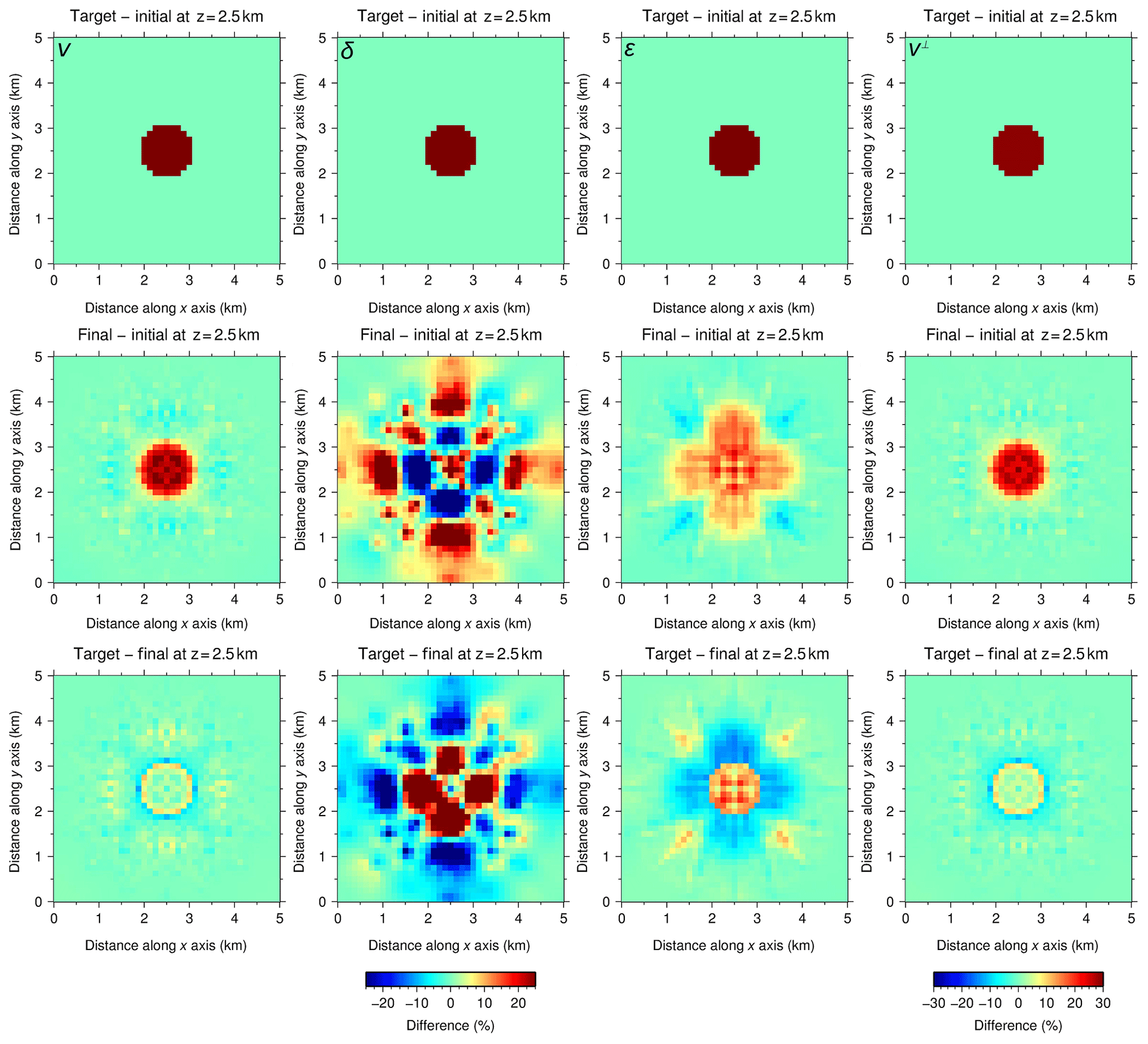
Figure 5 Simultaneous inversion with P[ε]. Horizontal slices of the relative differences between target and initial (first row), final and initial (second row), and target and final (third row) models at 2.5 km depth for the four parameters. v^⊥ is derived from Eq. (2). The range of the color scale for v^⊥ is wider than for the rest of parameters because the heterogeneity is calculated considering the 25 % anomalies in v and ε, which yields a ∼29.3 % anomaly in v^⊥. The first and second rows would be identical if the inversion were perfect, whereas the third row would display a homogeneous value of 0 %. The quality of the recovery of each parameter is correlated with their sensitivities (Fig. 2). Recovery of v is satisfactory, with anomaly values close to the target and well-defined anomaly boundaries. ε recovery is partial; the anomaly is centered but its magnitude and shape are not as accurate as in the case of both velocities; even so, it allows for a successful recovery of v^⊥ through Eq. (2), both in anomaly magnitude and shape. As for δ, recovery is unsuccessful.

Figure 6 Same as Fig. 5 but with P[v^⊥]. ε is derived from Eq. (2). The quality of the recovery is correlated with sensitivity (Fig. 2). Both velocities are satisfactorily recovered. The magnitude of the anomaly in v is better recovered than for P[ε], whereas the opposite occurs for v^⊥. Anomaly boundaries for both velocities are not as well determined as for P[ε]. ε and δ are not recovered.

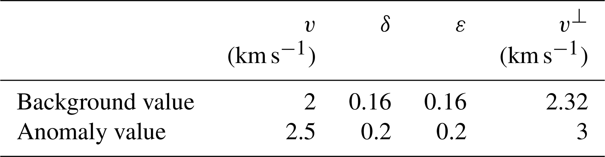
According to the definition of sensitivity, alternately for v, δ and ε, the said anomaly was added at the center of the cube representing a 25 % increase on the background value, while the models for the rest of parameters in the parameterization remained homogeneous. Table 1 summarizes the background and anomaly values for all parameters in each sensitivity test, along with their equivalence in the alternative parameterization. Since v is related to ε and v^⊥ through Eq. (2), its sensitivity pattern changes depending on the parameterization used (Fig. 2). Indeed, a 25 % increase in v with respect to equivalent background models in P[ε], and P[v^⊥] (Table 1) yields different sensitivities because of the different parameters involved (ε or v^⊥) in the representation of the medium. Contrarily, the δ sensitivity pattern is independent of the parameterization used. ε and v^⊥ sensitivities are only defined in their respective parameterizations. However, a 25 % increase in v^⊥ yields an equivalent ε of 0.45, which is greater than the ∼0.2 limit for weak anisotropy approximation. Thus, instead of establishing the comparison with v^⊥ sensitivity based on a proportional anomaly increment and measuring its effect on travel times, we based it on an equal travel-time change; i.e., the same change in travel time requires a change of 25 % in ε but only a ∼3.4 % change in v^⊥ (Table 1), indicating that data are ∼7 times more sensitive to v^⊥ than to ε changes.

Table 1 Values for anomaly and background areas of the models used in each of the four sensitivity tests and their equivalence in the alternative parameterization (italic values) (Fig. 2). Accuracy tests in Fig. 3 are conducted for these same four cases. A comparison with the accuracies achieved using the alternative parameterizations can be seen in Fig. S2.

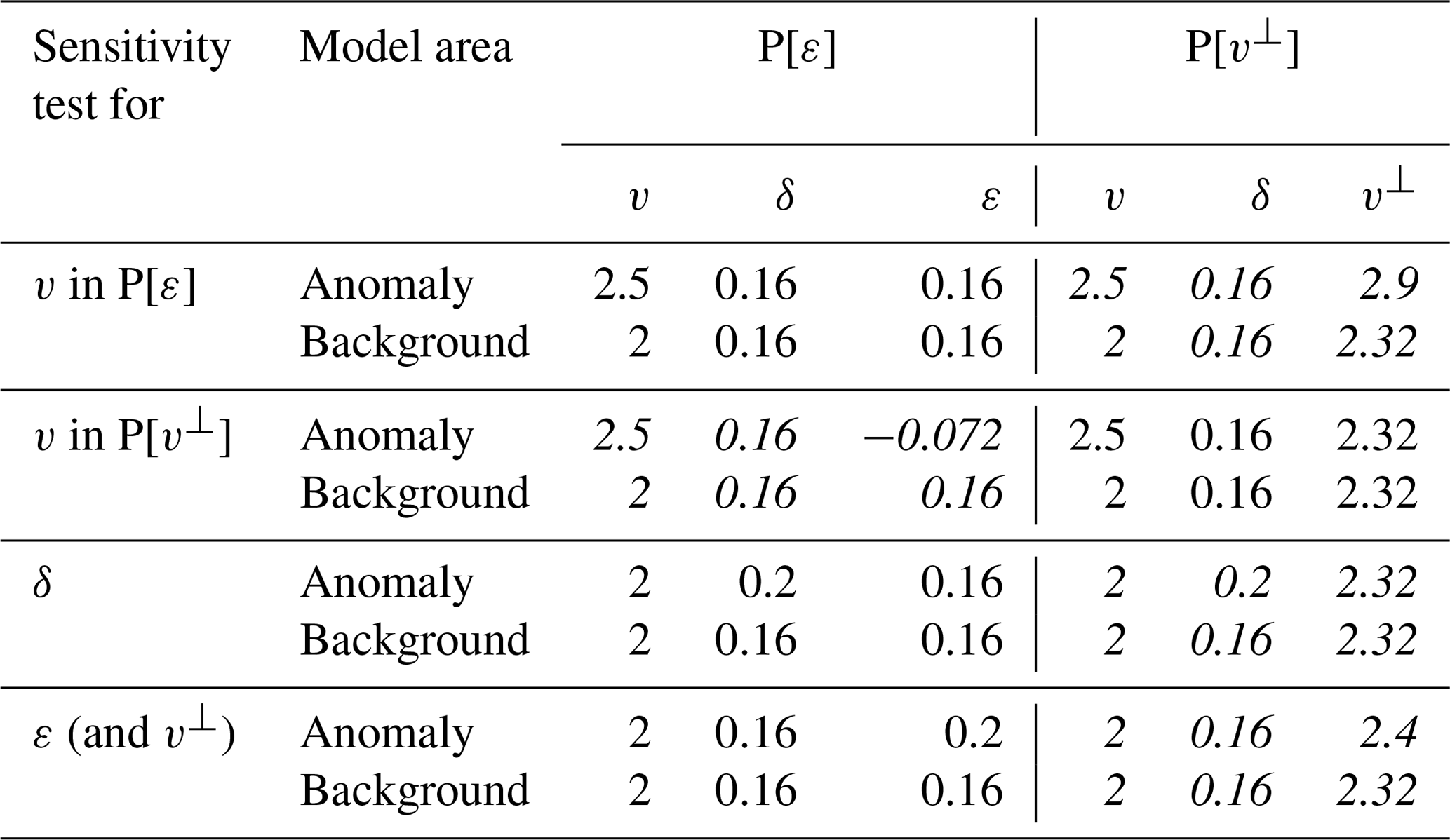
v sensitivity in P[ε] is the highest for all angles, 4.5 % to 5 % (Fig. 2), and it can be shown that expressed in its relative form, the analytic solution is a constant 5 % (see mathematical proof in the Supplement). In its normalized form, it follows the same sinusoidal pattern as in P[v^⊥] (Fig. 2e), and both have equal maxima in the directions parallel to the symmetry axis. In both cases, minima are found in the directions perpendicular to the symmetry axis, but in P[v^⊥] they reach down to 0, whereas in P[ε] the value is ∼0.85. As expected from Eq. (1), ε sensitivity goes to 0 % in the directions parallel to the symmetry axis and has its maxima (∼0.8 % or ∼0.15) for the polar angles perpendicular to it. v^⊥ sensitivity would follow the same angular dependence but with maxima of the order of magnitude of v sensitivities. Finally, δ sensitivity is, at its maxima, more than 1 order of magnitude smaller than v sensitivity, around 0.25 % or 0.05. These sensitivity results indicate that we can generally expect similar recoveries for v and v^⊥, better than for ε, and that retrieving δ might prove complicated. Keep in mind that these sensitivities for v, δ and ε are produced by an anomaly that represents a 25 % increase with respect to the background value, and that an anomaly in v^⊥ would produce the same sensitivity pattern as ε with only a ∼3.4 % increment.

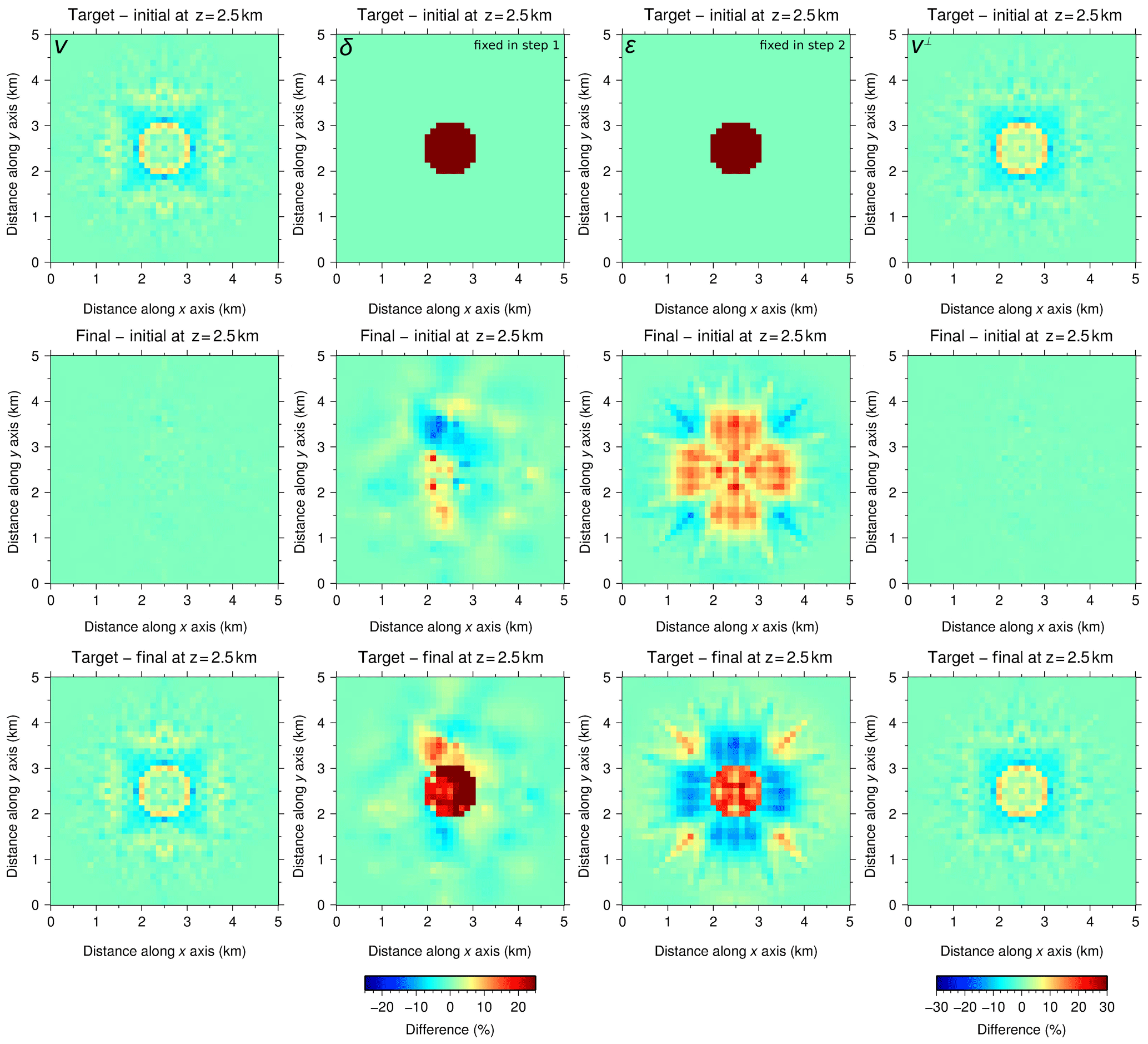
Figure 7 Same as Fig. 5 but for the two-step sequential inversion strategy with P[ε]. In the first step, only δ was fixed. In the second step, only ε was fixed. Final models from step 1 were used as initial models for step 2. v (first column) is well recovered in step 1 (top panels), and it is barely modified by the second step (middle and bottom panels). δ is fixed to the initial homogeneous model in step 1, and its recovery is unsuccessful in step 2. Recovery of ε is limited compared to v but significantly better than that of δ. Nonetheless, it proves to be good enough to provide a satisfactory recovery of v^⊥ using Eq. (2).

The differences in synthetic sensitivities between meridians arise from the discretization of the model space in a Cartesian system of coordinates. Such approximation inevitably defines privileged directions for ray tracing and consequently produces differences in synthetic travel times. The mismatch between synthetic and analytic sensitivities (Fig. 2) occurs because the discretization used cannot represent the surface of a perfect sphere. These effects are most notable in the v sensitivity, in P[ε] and to a lesser extent in P[v^⊥], precisely because it is the most sensitive parameter, and thus the errors in the representation of a sphere and the existence of privileged directions have a much larger influence on the calculated travel times. Figure S1 shows how refining the v model reduces the relative travel-time error (Fig. S1a in the Supplement) and generates a more accurate sensitivity pattern (Fig. S1b). In a real case study, one can always refine the grid spacing of a particular parameter to achieve better accuracy, but here we wish to test the performance of the code in the modeling and recovery of each parameter under the same conditions, i.e., equivalent anomalies and identical model discretization.

3.2 Accuracy

For the four simulations in the sensitivity analysis, we compared the synthetic travel times obtained with our code to the analytic solution to quantify the accuracy of the code's performance. The comparison along the two selected meridians at 0 rad and π∕4 rad azimuths is displayed in Fig. 3 expressed as relative travel-time error, i.e., the difference between synthetic and analytic travel times relative to the latter in percentage. Table 2 contains the mean of the relative travel-time errors and their respective mean deviations for these four tests and along the two selected meridians, as well as the overall values for each of them.

Figure 8 Same as Fig. 7 but for the two-step sequential inversion strategy with P[v^⊥]. In the first step, only δ is fixed, whereas in the second one all parameters are inverted. v (first column) and v^⊥ (fourth column) are well recovered in step 1 (top panels), and they are barely modified by the second step (middle and bottom panels). δ and ε are not properly recovered; in both cases, some sort of irregular perturbations approximately centered in the cube are retrieved but bear no resemblance to the target anomalies.

Table 2 Mean relative travel-time errors in percentage and their mean deviations for the two selected meridians in Fig. 3 and for the entire set of 482 source–receiver pairs. Compared to Fig. 2a–b, these average travel-time error values indicate that the code is sufficiently accurate to model the travel-time residuals arising from the inclusion of the selected anomalies.

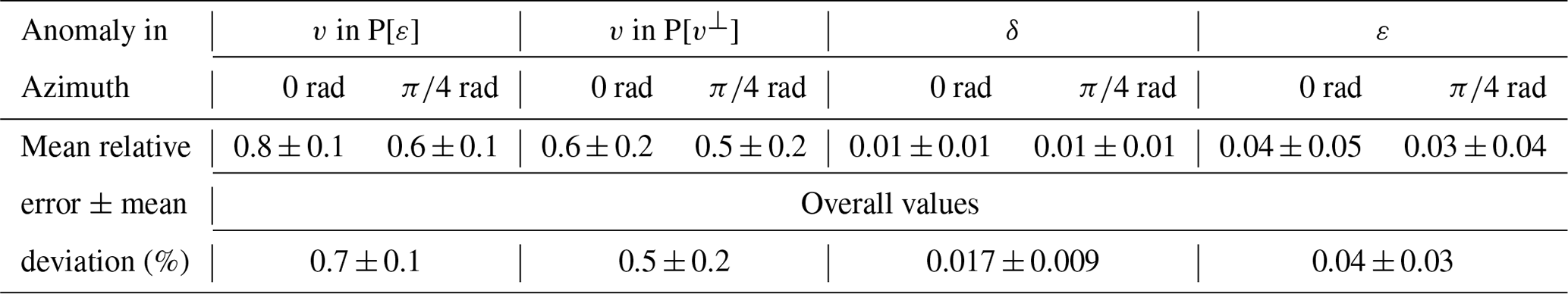
Comparison of Fig. 2a–b with the values in Table 2 and Fig. 3 indicates that the forward calculation of travel times is accurate enough with respect to the travel-time residuals expected for the selected anomalies. Sensitivity is at least 5 times and up to 2 orders of magnitude greater than travel-time accuracy errors depending on the parameters, with the exception of angles for which sensitivity tends to zero. Figure S2 illustrates that the code is able to reproduce nearly identical accuracies using both parameterizations. Furthermore, given that we are using the same synthetic travel times that we used for the sensitivity analysis, this also implies that the sensitivity patterns obtained with the alternative parameterization would be virtually equal to those in Fig. 2.

Figure 9 Same as Fig. 5 but using target models as initial models for all parameters in P[ε] but δ. This test was conducted to study the recovery of δ under unrealistically optimal circumstances, and even with these perfect initial conditions, recovery is, at best, extremely complicated due to the small sensitivity (Fig. 2); magnitude and shape are only partially recovered. In the first row, differences for v and ε are 0 % since we use target models as initial ones. For this same reason, the second and third rows show that differences between target and inversion for these three parameters are hardly observable, indicating that inversion is not modifying v and ε even though they are not fixed. Consequently, the resulting recovery of v^⊥ through Eq. (2) is almost perfect as well.

3.3 Inversion results

For the inversion tests, we considered a synthetic medium defined by the anomaly models of all four parameters. Here, we refer to these models as target models, and the goal of the inversion is to retrieve the heterogeneity in each of them. These tests are conducted for the two parameterizations of the anisotropic medium described in Sect. 2: P[ε] and P[v^⊥]. Note that, in order to perform the inversion tests on equivalent cases for both parameterizations, the heterogeneity in v^⊥ is calculated with Eq. (2) considering the 25 % anomalies in v and ε, which yield a ∼29.3 % anomaly in v^⊥ (Table 3). If not indicated otherwise, we use background models as initial models. Finally, we study the potential recovery of δ because inverting this particular parameter proves notoriously difficult due to its low sensitivity (Fig. 2).

Table 3 For inversion tests, background and anomaly values of all four parameters for the initial/background model and for the anomaly in the target model. The model is a cube of edge 5 km. The anomaly is a discretized sphere of 1 km in diameter at the center of the cube.

The synthetic data set is made of 114 sources, each recorded at 113 receivers for a total 12 882 first-arrival travel times. For the acquisition geometry, again sources and receivers are located at the surface defined by the sphere inscribed in the cube (Fig. 1). The 114 positions at the surface of this sphere are shared by sources and receivers, and each receiver records all sources, except for the one source located at its same position.

For both parameterizations, we compared two inversion strategies: simultaneously inverting for all parameters and a two-step sequential inversion. First, in Figs. 5 and 6, we show the best results for the simultaneous inversion strategy. For each parameterization, we derived the fourth parameter by applying Eq. (2).

Table 4 shows several statistical measures to quantify the quality of these inversion results. As a measure of data fit improvement, we provide the root mean square (rms) of travel-time residuals for the first and last iterations. As a measure of model recovery or fit, for each parameter, we calculate the mean relative difference for the background area between the inverted model and either the target or the initial one, as they are identical in this area, as well as for the anomaly area comparing the inverted model to both the target and the initial models. In the case of a perfect recovery, mean relative difference for the background area would be 0 %, whereas for the anomaly area, it would be 0 % when using the target model as a reference and 25 % (∼29.3 % for v^⊥) when comparing to the initial model.

Table 4 Quantification of the quality of recovery in terms of data and model fit for the simultaneous inversion of both parameterizations (Figs. 5 and 6). Initial and final rms values for travel-time residuals to quantify data fit. For each parameter, as a measure of model fit, we computed the mean relative differences between the background areas of the inverted and target models (BG), the anomaly areas of the inverted and initial models (AI), and the anomaly areas of the inverted and target models (AT). Since the initial model is equal to the target model in the background area, it is not necessary to calculate the difference between inverted and initial models for this area. The ideal difference value for BG is 0 %. AT and AI indicate the resemblance between true and recovered anomalies, and their ideal values are 0 % and 25 % (∼29.3 % in the case of v^⊥), respectively. Recovery is consistent with sensitivity (Fig. 2): v and v^⊥ are well retrieved, ε is only partially recovered with P[ε], whilst inversion of δ is unsuccessful in both cases.

In an attempt to improve the recovery of δ, we repeated these two tests for different values of the smoothing constraints, but it proved impossible. Correlation lengths tested for all four parameters include 0.25 km (twice the grid spacing), 0.5 and 1 km. The weights of the smoothing submatrices for each parameter, λ in Eq. (3), were varied between 1 and 100, with intermediate values of 2, 5, 10, 20, 30 and 60. For successful inversions, very similar results for the other parameters were obtained regardless of the final δ model. In other words, the low sensitivity of δ makes it extremely hard, if not impossible, to recover this parameter from travel-time data, but for this same reason it has little or no influence on the recovery of v and ε or v^⊥.

The two-step sequential inversion strategy was also tested for both parameterizations, P[ε] and P[v^⊥]. For the first step, we tested two options: (a) inverting for v while fixing δ and ε or v^⊥ and (b) fixing only δ. In the second step, we used the inverted models from step 1 as initial models and tested three options: (c) inverting for all three parameters, (d) fixing only δ, when following option (a) in step 1, and (e) fixing v and/or εor v^⊥, when following option (b) in step 1. Figure 4 shows a flowchart describing all the sequential inversion combinations tested. Again, smoothing constraints were varied for similar correlation lengths and submatrix weights as detailed for the simultaneous inversion case.

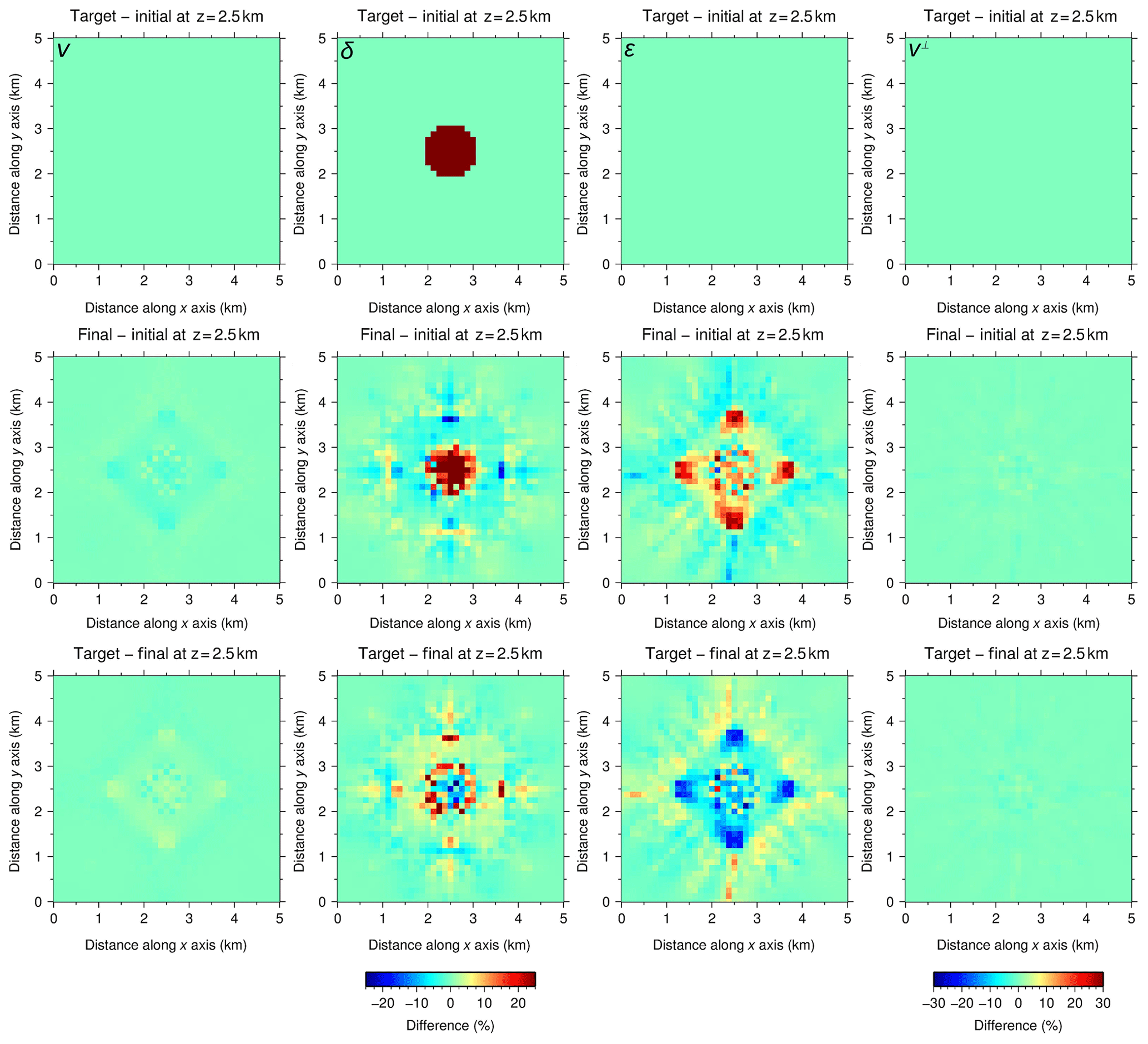
Figure 10 Same as Fig. 9 but using target models as initial models for all parameters in P[v^⊥] except for δ. The magnitude of the δ anomaly is better recovered than for P[ε], but the shape is not as well retrieved, and artifacts appear in the background area. Differences between inverted and target v and v^⊥ models are still hardly observable but not as much as for v and ε in the case of P[ε], and thus the recovery of ε through Eq. (2) is also not as good.

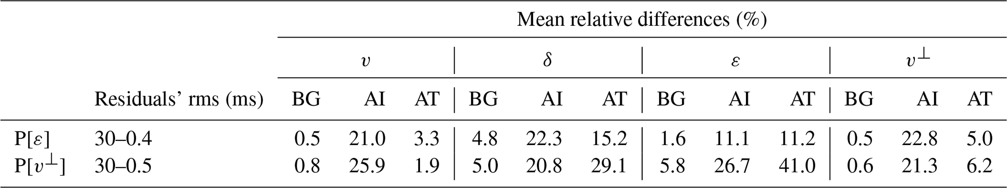
As indicated in Fig. 4, in the case of P[ε], the best result (Fig. 7) was obtained inverting for v and ε while fixing δ in the first step and fixing only ε in the second step, whereas for P[v^⊥], the best combination for the two-step inversion (Fig. 8) was fixing only δ in step 1 and inverting for the three parameters in step 2. Tables 5 and 6 summarize the statistical quantification of data and model fit for each parameterization.

Table 5 Same as Table 4 but for the two-step sequential inversion of P[ε] (Fig. 7). Recoveries in terms of model fit are virtually identical to those for the simultaneous inversion of this parameterization, with ε recovery being just slightly better. Final data fit is also better than the one achieved by simultaneous inversion of P[ε].

Table 6 Same as Table 5 but for the two-step sequential inversion of P[v^⊥] (Fig. 8). Model fits are similar to those achieved by the simultaneous inversion of this parameterization: v and v^⊥ are well retrieved, while recovery of δ and ε is unsuccessful. Final data fit is identical to the one obtained by simultaneously inverting for P[v^⊥].

3.4 Modeling δ

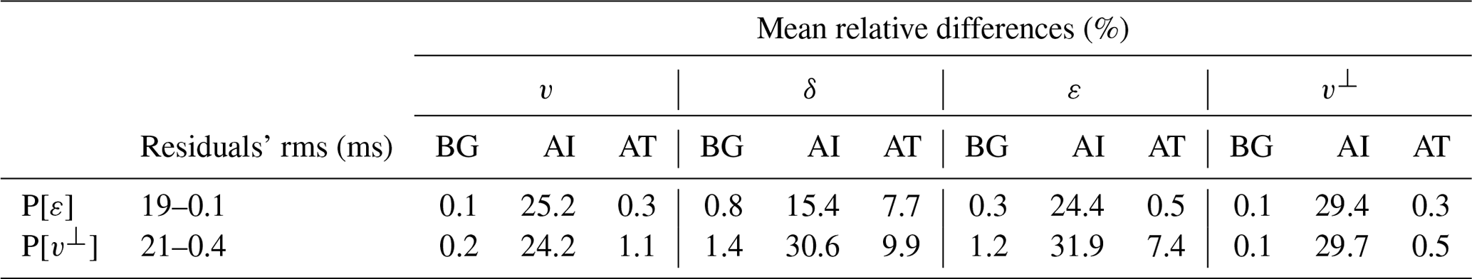
Observing that good results for v and ε or v^⊥ are achieved regardless of the result in δ and knowing that the sensitivity of δ is notably smaller than that of the other parameters, we explored a strategy to have an estimate of this parameter. First, as a reference, we considered an unrealistically optimal scenario in which the real v and ε or v^⊥ models are known to us. Figures 9 and 10 show the resulting δ achieved by repeating inversions in Figs. 5 and 6 with v and ε or v^⊥ target models as initial models. Table 7 summarizes the travel-time residuals' rms and the mean relative difference for each parameter in these inversions. Again, these two tests were repeated for ranges of smoothing constraints in all four parameters, as described for the cases in Figs. 5 and 6. Table 7 and Figs. 9 and 10 correspond to the best results obtained, which indicate that the recovery of δ is, at best, extremely complicated due to the limited sensitivity of travel-time data to changes in this parameter.

Table 7 Same as Table 4 but for the simultaneous inversion of P[ε] and P[v^⊥] using v and ε or v^⊥ target models as initial models (Figs. 9 and 10). Model fits for v and ε or v^⊥ are close to perfect as expected, but even so the recovery of δ is partial at most. Data misfit is smaller than for the original inversions in Figs. 5 and 6. P[ε] yields a better result according to all indicators, and as for all previous tests, the recovery of v^⊥ from P[ε] is notably better than that of ε from P[v^⊥].

Next, we decided to try neglecting δ in Eq. (1), and we repeated a number of inversions, such as the ones displayed in Figs. 5 and 6, following

$$\begin{array}{}\text{(11)}& v^{\mathrm{a}}\left(v,\mathit{\epsilon },\mathit{\theta }\right)=v\cdot \left(\mathrm{1}+\mathit{\epsilon }\cdot {\sin }^{\mathrm{4}}\left(\mathit{\theta }\right)\right).\end{array}$$

The purpose of these tests was checking whether it was possible to invert v and ε or v^⊥ with data generated following Eq. (1) using the approximation in Eq. (11), given that the influence of δ on the results for other parameters is rather small, that δ cannot be accurately retrieved from travel time alone and that it has the smallest sensitivity. To do so, a homogeneous model of δ=0 was fixed throughout the inversions. These tests were unsuccessful, with noticeably poorer results than when considering a dependence on δ (Table 8). However, they were useful in proving that even if a detailed δ model is not necessary to successfully retrieve the other parameters, at least a rough approximation of the δ field is needed to recover the other parameters, e.g., the background δ model that we used as the initial model in inversions displayed in Figs. 5 and 6.

Table 8 Same as Table 4 but for the simultaneous inversion of P[ε] and P[v^⊥] following Eq. (1), i.e., neglecting δ in Eqs. (1) and (3). Model differences for v, ε and v^⊥, as well as data misfit, are all significantly worse than for any of the previous tests.

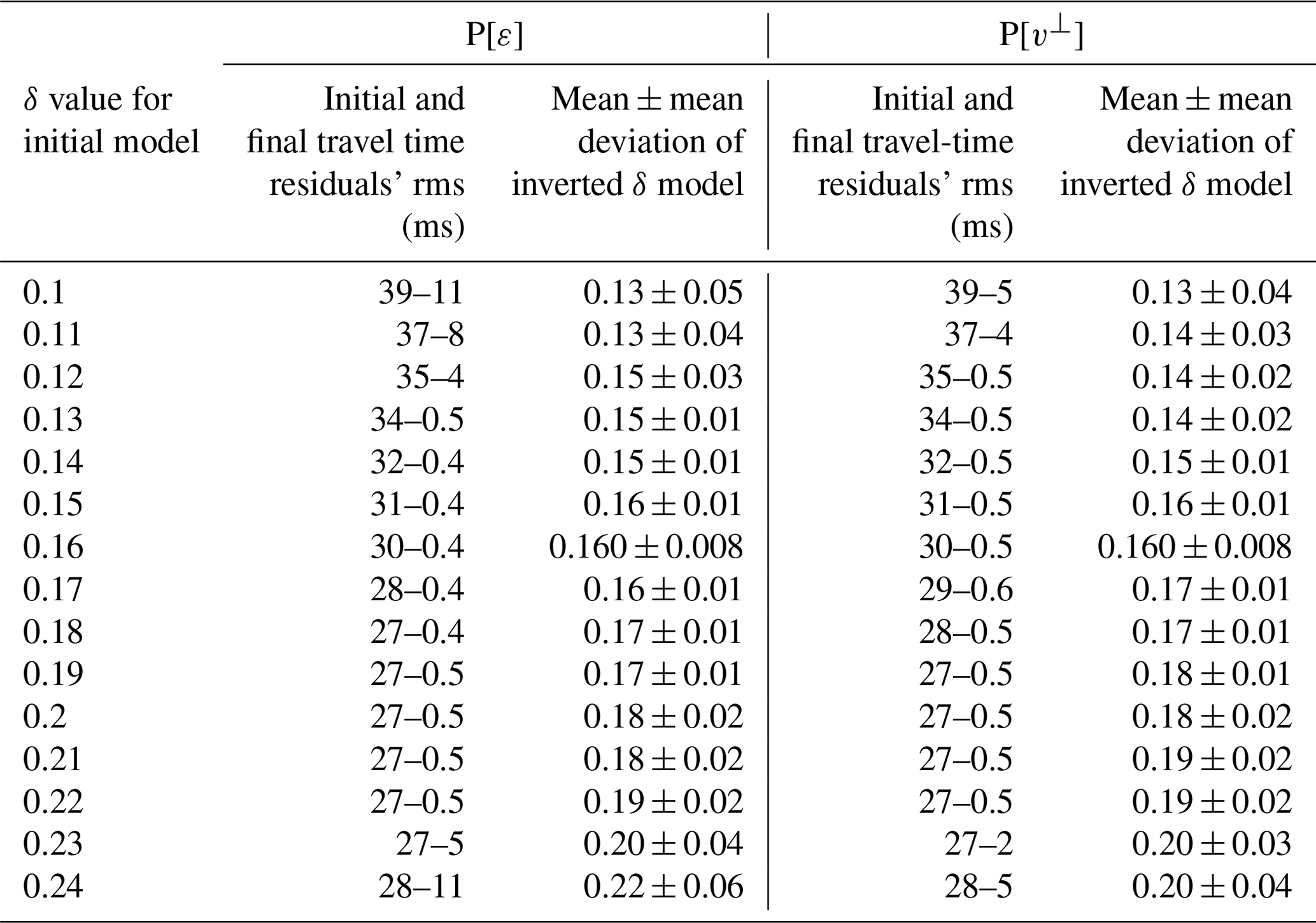
Finally, we tested whether it would be possible to obtain at least this rough approximation of δ in the medium, valid in the sense that it allows for the successful recovery of the rest of parameters, using any a priori information available such as compilations of anisotropy measurements (e.g., Thomsen, 1986; Almqvist and Mainprice, 2017). Once again, we repeated inversions from Figs. 5 and 6 (initial δ=0.16), now using different homogeneous initial models for δ within a range of possible values from 0.1 to 0.24. Table 9 contains the initial and final rms of travel-time residuals, as well as δ mean values for the inverted model along with the corresponding mean deviations. It is straightforward to note that, for a central subrange of the tested initial δ values, final rms values are an order of magnitude smaller, a few tenths of a millisecond compared to the few milliseconds outside this subrange. Specifically, very similar results to those in Figs. 5 and 6 in terms of travel-time, residuals' rms are produced by initial δ values between 0.13 and 0.22 for P[ε], and between 0.12 and 0.22 for P[v^⊥]. The narrowing of the initial δ distribution to a smaller subrange of mean δ values for the inverted models is indicative of a good general convergence trend.

Table 9 Results of the procedure to approximate an initial δ model. The rms of the final travel-time residuals shows a clear change in order of magnitude in the subranges (0.13, 0.22) and (0.12, 0.22) depending on the parameterization. Results for initial δ=0.16 correspond to the examples in Figs. 5 and 6.

The rough estimate of the δ field could be built, for instance, as the average of the mean δ values for the inverted models in the central subranges defined by the change in magnitude of the final rms of travel-time residuals. One final inversion could be run using a homogeneous initial δ model with this average value, with the additional option of fixing it and inverting only for the other two parameters. As mentioned in Sect. 2.2, potentially more detailed initial δ models could be obtained from the normal move-out correction of near-vertical reflection seismic data.

3.5 Discussion

We have tested two parameterizations of the VTI anisotropic media, P[ε] (v, δ, ε) and P[v^⊥] (v, δ, v^⊥), and two inversion strategies, simultaneously inverting for all three parameters and a two-step sequential process fixing some of the parameters in each step. We consider three criteria for evaluating and comparing the quality of the inversion results obtained following the four possible combinations of strategies and parameterizations: visual inspection of the results, as well as travel-time data and model fits. For both inversion strategies and both parameterizations, the recovery of the parameters is positively correlated with their respective sensitivities; the more sensitive parameters are systematically better recovered.

For the simultaneous inversion, both parameterizations were able to produce acceptable final results (Figs. 5 and 6). According to our tests, P[ε] provides the best outcome, specifically because data and model fits (Table 4) are better for this option but, more importantly, because of the difference in the quality of the recovery of ε. However, visual comparison of the recovery of v as well as the v model fit in Table 4 indicates that P[v^⊥] yields a slightly better result regarding the magnitude of the anomaly for this parameter, as is particularly evident at its center. In P[ε], given the disparity in sensitivities between v and ε, the former might be prone to accounting for data misfit that actually corresponds to the latter, whilst in P[v^⊥] this disparity is less acute. The boundaries of the anomalies for both velocities are still better retrieved with P[ε]. Also, the recovery of δ, even though it is far from acceptable, is significantly better in the case of P[ε]. This might be explained because the disparity of δ sensitivity is greater with respect to the other two parameters in P[v^⊥] than in P[ε].

In general, sequential inversion is a more complex process that requires more human intervention and fine tuning in each step. In addition, fixing some of the parameters in the first step may result in the inverted parameters artificially accounting for part of the data misfit that is actually related to the fixed ones. This can more easily lead convergence into a local minimum, and it might be impossible to correct this tendency in the second step. For this inversion strategy, it is also P[ε] that produces the best results (Figs. 7 and 8). Data fit and the model fit of ε are slightly better than for the simultaneous inversion of this parameterization (Tables 4 and 5), whereas model fits and the visual aspect of both velocities are almost identical to those obtained by simultaneously inverting all three parameters (Figs. 5 and 7). Visually, it is difficult to decide whether the recovery of ε is better or not than for the simultaneous inversion (Figs. 5 and 7). As for δ, recovery is unsuccessful and artifacts appear in the background area of the model but, according to both its model fit and its visual aspect, it is notably better than for the simultaneous inversion. As in the case of simultaneous inversion, the only advantage of using P[v^⊥] instead of P[ε] is that it yields a better recovery of the anomaly magnitude of v (Tables 4 and 6). The results for both velocities are virtually identical to those obtained by simultaneous inversion of this parameterization (Figs. 6 and 8). δ and ε are not properly retrieved, but the results are significantly better than for the simultaneous inversion of this same parameterization.

δ has been shown to be by far the most complicated parameter to retrieve because of the low sensitivity of travel time to its variation (Fig. 2). Even when excellent v and ε or v^⊥ models are available, i.e., the target models for these parameters in our synthetic tests, the recovery of δ is limited at best (Figs. 9 and 10 and Table 7). However, and for the same reason, poor recoveries of δ do not affect the recovery of the other two parameters, meaning that a detailed δ model is not necessary to satisfactorily retrieve v and ε or v^⊥ (Figs. 5–10). Still, our inversion tests also proved that neglecting δ in Eqs. (1) and (3) is not an option, the accuracy in the recovery of the other parameters resulting severely affected (Table 8). Thus, even if a detailed inversion of δ is, at the very least, hard to achieve, and it is not needed for a successful result in the other parameters, some sort of simple, even homogeneous, initial δ model with a value or values about the average δ in the medium is necessary for a good recovery of the other parameters.

We showed that given some a priori information on the range of possible δ values in the medium, it should be possible to create the necessary initial δ model. In order to illustrate this, we chose a range of δ values for the initial model and reran the inversions in Figs. 5 and 6. The results indicate that for any homogeneous initial δ model in a certain subrange close to the actual average δ value of the medium, the results for v and ε or v^⊥ are satisfactory and virtually identical to those of the original inversions (Table 9). This subrange is easily defined by looking at the final rms of travel-time residuals, which experiences a notorious change of 1 order of magnitude. Any model within this subrange works similarly well as an initial δ model. Alternatively, a possibly more robust selection of the constant value for a homogeneous initial δ model might be the mean (or also the median or the mode) of the mean δ values for the inverted models in this subrange. It is worth noting that, whereas for the purpose of this work we used the same discretization for all parameters, in a real case study it would probably be recommendable to use a coarser discretization for δ than for the other parameters and in general a finer discretization for the more sensitive parameters (Fig. S1). Indeed, a heterogeneity of a given spatial scale and relative variation will produce a greater effect on data for a parameter of greater sensitivity. Thus, for a parameter of greater sensitivity, it will be easier for the code to identify smaller heterogeneities both in scale and variation, which will require a finer grid.

4 Conclusions

We have successfully implemented and tested a new anisotropic travel-time tomography code. For this implementation, we had to modify both the forward problem and the inversion algorithms of the TOMO3D code (Meléndez et al., 2015b). The forward problem was adapted to compute the velocities observed by rays considering Eq. (1) for the weak VTI anisotropy formulation in Thomsen (1986). The inversion solver was extended to include the δ, ε and v^⊥ kernels in the linearized forward problem matrix equation, as well as smoothing and damping matrices for these parameters defined following the same scheme as for velocity in the isotropic code (Eqs. 3–10).

Regarding the synthetic tests, we first determined the sensitivity of travel-time data to changes in each of the parameters defining anisotropy in the medium (v, δ, ε, v^⊥) (Fig. 2), and we checked the proper performance of the code by comparing the synthetic travel times produced with their respective analytic solutions (Fig. 3). Next, we performed canonical inversion tests to compare two possible media parameterization, P[ε] and P[v^⊥], and two possible inversion strategies, simultaneous and sequential. According to our tests, both parameterizations have their strengths: P[ε] produces the best overall result in the sense that all parameters are acceptably recovered, with the exception of δ, and trade-off between parameters is lower, but P[v^⊥] yields the best result for the magnitude of the anomaly in v. Regarding the inversion strategy, simultaneous inversion is more straightforward and involves less human intervention, and given that both strategies yield similar results, it would be our first choice. Sequential inversion is always a more complex process that can be shown to work in a synthetic case because the target models are available, but in field data applications the complexity would most likely be unmanageable. These tests were conducted under ideal conditions, and thus the conclusions provided by their results are an upper limit but generalizable estimation of the strengths and weaknesses in the code's performance.

An acceptable recovery of δ turned out to be impossible due to the small sensitivity of travel times to this parameter, but we verified that it cannot simply be neglected in the equations. Whereas the recovery of the other parameters is not significantly affected by that of δ, a rough estimate of the average δ value in the medium is necessary and sufficient to generate a homogeneous initial model that allows for satisfactory inversion results in these other parameters. We also proved that it is possible to obtain it, provided that some a priori knowledge on δ values in the medium is available to define a range of plausible values, such as field or laboratory measurements.