the Creative Commons Attribution 4.0 License.
the Creative Commons Attribution 4.0 License.
 | 08 Nov 2019
Extracting small deformation beyond individual station precision from dense Global Navigation Satellite System (GNSS) networks in France and western Europe
Christine Masson
Stephane Mazzotti
Philippe Vernant
Erik Doerflinger
We use 2 decades of data from a dense geodetic network to extract regionally coherent velocities and deformation rates in France and neighboring western European countries. This analysis is combined with statistical tests on synthetic data to quantify the deformation detection thresholds and significance levels. By combining two distinct methods – Gaussian smoothing and k-means clustering – we extract horizontal deformations with a 95 % confidence level of ca. 0.1–0.2 mm yr−1 (ca. 0.5– yr−1) on spatial scales of 100–200 km or more. From these analyses, we show that the regionally average velocity and strain rate fields are statistically significant in most of our study area. The first-order deformation signal in France and neighboring western European countries is a belt of N–S to NE–SW shortening of ca. 0.2–0.4 mm yr−1 (1– yr−1) in central and eastern France. In addition to this large-scale signal, patterns of orogen-normal extension are observed in the Alps and the Pyrenees, but methodological biases, mainly related to GPS (Global Positioning System) solution combinations, limit the spatial resolution and preclude associations with specific geological structures. The patterns of deformation in western France show either tantalizing correlation (Brittany) or anticorrelation (Aquitaine Basin) with the seismicity. Overall, more detailed analyses are required to address the possible origin of these signals and the potential role of aseismic deformation.
- Article
(30818 KB) - Full-text XML
-
Supplement
(7915 KB) - BibTeX
- EndNote


The Global Navigation Satellite System (GNSS) is a primary dataset to study present-day crustal deformation, for example through the computation of strain rate tensors, in active tectonics areas (e.g., Indonesia or Greece; Gunawan et al., 2019; Chousianitis et al., 2015) and in very low-deformation areas (e.g., eastern Canada or India; Tarayoun et al., 2018; Banerjee et al., 2008), as well in volcanic areas (e.g., Etna; Palano et al., 2010). However, the analysis of regional and local deformation is commonly restricted by several factors, such as the precision of individual GNSS velocities, the presence of non-tectonic transient signals or the methods used to compute strain rates on different spatial scales (e.g., Cardozo et al., 2009; Zhu et al., 2011; Carafa and Bird, 2016). In particular, the precision of individual GNSS velocities is a strong limitation in intraplate regions, where the amplitude of the tectonic signal is of the same order of magnitude as the measurement uncertainties (e.g., Calais and Stein, 2009; Tarayoun et al., 2018). The lengthening of time series and the increase in the number of stations makes it possible to better constrain deformation in the intraplate domains (e.g., Kreemer et al., 2018; Tarayoun et al., 2018).
In this study, we evaluate the ability to extract regionally coherent and statistically significant information on the present-day deformation rates in France and neighboring western European countries from GNSS networks. This analysis is performed in several stages. (1) We first compute a consistent velocity dataset based on GPS (Global Positioning System) signals for over 900 stations, using statistical semiautomatic techniques for time series processing (in particular offset and outlier detections). (2) The GPS velocities are analyzed using two independent methods (k-means clustering and Gaussian smoothing) in order to extract coherent velocities and deformations on spatial scales of 100–200 km. (3) We perform Monte Carlo and bootstrap sampling analyses on the original GPS velocities and on synthetic velocity data to estimate the detection threshold and the significance level of the computed velocity and strain rate fields.
Our study is focused on France and neighboring western European countries since they represent an ideal location for testing these methodological developments. Indeed, they are often considered as a domain without significant deformation except in its bordering mountain ranges, the Alps (e.g., Houlié et al., 2018; Brockmann et al., 2012; Tesauro et al., 2006) and the Pyrenees (e.g., Neres et al., 2018; Rigo et al., 2015). The Alps and Pyrenees have a high level of seismic activity (Fig. 1), allowing us to study how it relates to the GPS deformation rates, both in spatial distribution and style. The rest of France experiences a low to moderate diffuse seismicity in many regions (Cara et al., 2015; Fig. 1) suggesting that it undergoes a small but non-zero present-day deformation. We show that, in most of our study area, horizontal deformation rates can be estimated from GPS data with a 95 % confidence level of ca. 0.1–0.2 mm yr−1 (ca. 0.5– yr−1) on a spatial scale of 100–200 km or more. We discuss the relationship between the observed deformation and regional seismicity and neotectonic indicators. These interpretations are preliminary, and for several regions a specific and in-depth study is necessary.
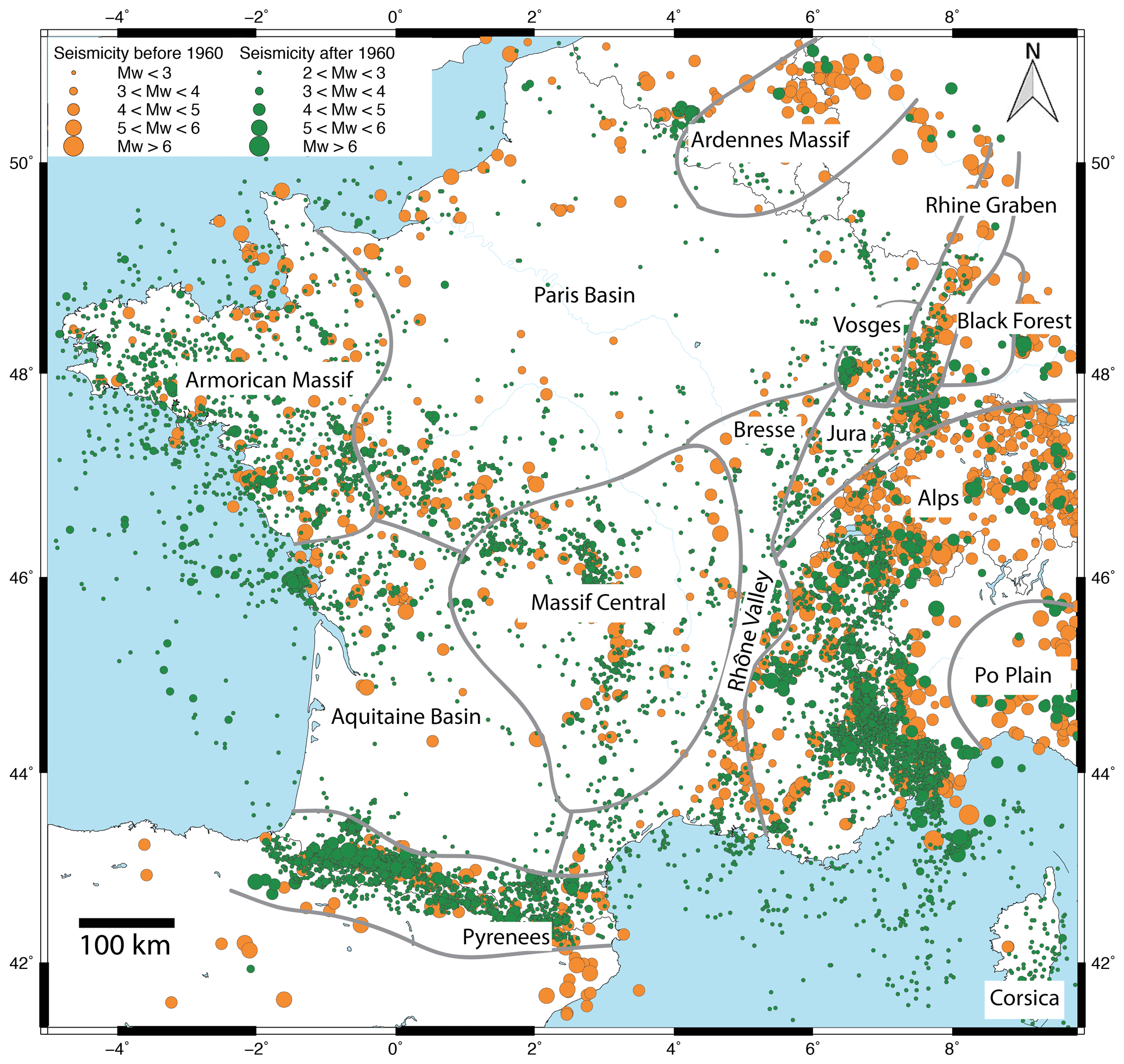
Figure 1Map of instrumental in green and historical in orange seismicity (SHARE (Seismic Hazard Harmonization in Europe) and SI-Hex (Sismicité Instrumentale de l’Hexagone)). Gray lines delimit the main geological areas.
We process data of 987 GNSS stations over a period ranging from 1998 to the end of 2016. The calculation was extended to a wider area than the frame considered in the rest of this study. Thus 313 stations mainly in Italy and Spain do not appear on France-centered maps. Table S1 in the Supplement shows the velocities of all stations used in the calculation. The time series cover time spans from 1.5 to 19 years with an average duration of 7 years. Not all stations have been installed under the same conditions and with the same goals (geodetic, cadastral, etc.). About a quarter of the stations are installed and maintained by private networks, for which we do not have all the information on the site monumentation or history of equipment changes. Figure 2 shows the distribution of these stations and identifies the additional campaign stations and Swiss stations combined with the main dataset (Sect. 2.4).
For data processing, we use the Precise Point Positioning (PPP) software developed by the Canadian Geodetic Survey of Natural Resources Canada (CSRS-PPP v1.05) (Héroux and Kouba, 2001). Optimum processing parameters and options to compute 24 h average daily positions are defined by Nguyen et al. (2016), following International GNSS Service (IGS) products and recommendations (Kouba et al., 2009; Dow et al., 2009). We use the IGS Final Products for satellite orbits and clocks, satellite and ground antenna absolute phase center mapping, and Earth rotation parameters. We also use standard models for tropospheric delay corrections (VMF1, Boehm et al., 2006) and solid Earth and ocean tide loading corrections (FES 2004, Lyard et al., 2006).
2.1 Time series analysis
Daily position time series are modeled with a constant velocity, annual and semiannual periodic motions, instantaneous offsets, and random colored noise:
where x is the daily position, t is the time, v is the velocity, A1,2, ω1,2 and φ1,2 are the amplitudes, periods and phases of the annual and semiannual motions, Ci and Ti are the amplitude and date of the ith offset (with H the Heaviside function), and ε is the residual. To jointly estimate these parameters (except for the noise parameter), we use a linear least-square inversion of the model (Eq. 1).
Because many stations are associated with incomplete equipment logs that could provide position offset dates, the dates of potential offsets are automatically detected according to the method described in Masson et al. (2019a). Their statistical analysis shows that this method compares favorably with most automatic and manual detection methods (Gazeaux et al., 2013), with an average detection level of about 52 % vs. about 20 % of false positives. Overall, using this method results in horizontal (or vertical) velocity biases that are smaller than 0.2 mm yr−1 (or 0.5 mm yr−1) at 95 % confidence levels for series longer than 8 years. For series with a duration of between 4.5 and 8 years and no offset, the velocity biases are smaller than 0.3 mm yr−1 (horizontal and vertical) at 95 % confidence levels, and, if at least one offset is present, the velocity biases are 0.6 mm yr−1 (or 1.3 mm yr−1). For the shortest series (less than 4.5 years), the velocity biases are larger than 1.0 mm yr−1 (Masson et al., 2019a).
We calculate the velocity standard errors using Williams et al. (2003) generic expression for colored noise with a non-integer spectral index. The spectral index and amplitude of the colored noise are estimated using a least-square inversion of the residual (ε, Eq. 1) spectrum limited to periods between 1∕12 and T∕2 years (with T the length of the time series). This simple approach only provides a first-order estimation of the noise parameters and velocity standard errors (compared to a more complex nonlinear method, such as maximum likelihood). In agreement with other recent studies (Santamaria-Gomez et al., 2011; Nguyen et al., 2016), we observe that the spectral indices vary from −0.8 to −0.4, indicating a combination of white and flicker noise. Using synthetic time series analyses, Masson et al. (2019a) show that the simple “least-square spectrum” approach yields estimations of velocity standard errors that are reasonable for series with a spectral index smaller than −0.6 but that are underestimated for series with a spectral index greater than −0.4. The latter corresponds to only 18 % of our data, allowing us to have confidence in the calculated velocity standard errors.
2.2 Common-mode spatial filtering
In order to identify and correct for non-tectonic transient signals and noise common to the whole network, we define a common-mode correction (Wdowinski et al., 1997) by stacking the residual time series of 31 stations with near-complete data and durations greater than 17 years. Such a correction typically allows adjusting for network-wide biases such as systematic orbit and clock issues due to the IGS combination process or potential large-scale environmental loads. On average, the application of the common-mode correction to all stations reduces the daily dispersion on the North, East and Up components from 1.94 to 1.36 mm (−30 %), 2.49 to 2.07 mm (−17 %) and 4.54 to 4.12 mm (−9 %), respectively. The stacked time series show a decrease in dispersion of the North and East components between 1998 and 2002 (see Fig. S1 in the Supplement), which is likely related to improvements in IGS satellite ephemerids and reference frame definition (Griffiths, 2019). The latter can be observed on the North, East and Up components directly at or shortly after the transitions to IGS08 and IGb08 reference frames (see Fig. S1).
Pluri-annual signals with amplitudes of 1–5 mm over periods of 2–5 years are evidenced in the North, East and Up components (e.g., 2008–2011). Similarly, residual annual and semiannual signals are also detected despite the integration of these periodic motions in the time series model (Eq. 1). These residual signals indicate the presence of coherent phenomena operating over large geographical scales (100 s km) with varying durations, regularities and cyclicities. Longer series are required to confirm the presence of decadal or pluri-decadal (periods 10–15 years) signals, which could impact the estimations of long-term velocities.
2.3 Reference frame
After PPP processing and the application of the regional common-mode correction, daily positions and velocities are in an informal reference frame tied to the IGS satellite orbits and clocks (IGb08). In order to analyze the relative motions and deformations in France and conterminous western European countries, we rotate the velocities in a local frame, first using the Eurasia-ITRF2014 rotation defined by the ITRF2014 (Atamimi et al., 2016) and then minimizing the residual velocities of 200 stations distributed evenly over our region of interest and with time series duration greater than 7 years (Fig. 2).

Figure 2Distribution of the permanent (blue circles and blue circles with red outline for the stations used to define the “France-centered” reference frame) and campaign (pink triangles) stations used in this study. Green squares are combined Swiss stations.The red frame corresponds to the study area.
In this “France-centered” reference frame, two regional-scale systematic motions are detected in the velocity field (see Fig. S2). In northwestern Spain, a northward motion of ca. 0.1–0.3 mm yr−1 may be associated with the clockwise rotation of Iberia relative to Eurasia described by Palano et al. (2015) and Neres et al. (2016). This motion is not observed in the northeastern part of Spain, likely reflecting the location of the rotation pole and the specific dynamics of the Pyrenees (see Sect. 5.2). In northern Italy, the northern motion increasing eastward from 0 to ca. 3 mm yr−1 is compatible with the counterclockwise rotation of the Adria microplate relative to Eurasia, with a rotation pole located in the Po Plain (Battaglia et al., 2004; Farolfi et al., 2015). These tectonic movements are beyond the scope of our study.
2.4 Network densification
In order to densify the velocity field, we integrate data from additional networks (including campaign data) that were either processed or analyzed with a different procedure from the main dataset.
2.4.1 The Swiss network
Raw GNSS data (RINEX) are not available for Swiss stations, leading us to directly combine the processed velocities (http://pnac.swisstopo.admin.ch/restxt/, last access: 25 April 2019) with ours. We perform a six-parameter Helmert transformation (rotation and translation rates without scale) to minimize the residual velocities at the 58 sites common to the two datasets. Post-transformation statistics indicate an average agreement for the common sites of 0.15, 0.13 and 0.37 mm yr−1 in the North, East and Up components. The Swiss velocities include both campaign and permanent station velocities, for which the uncertainties are estimated with an unspecified method (Brockmann et al., 2012). These uncertainties are much lower than ours, requiring a first-order scaling to homogenize the two datasets. By comparing the distributions of uncertainties of the 58 common sites between the two solutions, we estimate a multiplication factor 24 for the North and East components and 20 for the Up component, to adjust the distribution of Swiss uncertainties to ours. This simple scaling yields a good first-order agreement of the two distributions (based on the 10, 50, and 90 quantiles), but detailed analysis still points out residuals issues that affect the interpretation of the combined field (see Sect. 5.3).
2.4.2 Campaign data
For the French Alps, we include campaign data from sites measured for at least 48 h during surveys in 1998, 2004, 2015, 2017 and 2018. The characteristics of the shortest and longest time series are 14 years with 2 surveys and 21 years with 5 surveys. In 1998 and 2004, measurements were made on tripods, while since 2015 the sites have been modified to use an anchored mast in order to optimize installation stability and antenna height measurement. We use the same data processing for 24 h daily positions as for permanent stations but the time series analysis is different. Since the data are sporadic (a few points every 4–10 years), it is impossible to model annual and semiannual seasonal signals, detect offsets and estimate noise characteristics by spectral analysis. No common-mode has been removed from the campaign data as the effect is not significant (Tarayoun et al., 2018). A careful re-analysis of the antenna heights and RINEX data allows us to estimate a long-term velocity (including daily position weighting by the measurement duration) for 29 sites in the French Alps (Fig. 2).
In the Pyrenees, campaign data extend from 1992 to 2017, but because of the relatively low quality of satellite orbits and clocks in the early and mid 1990s (Griffiths, 2019), data before 1996 cannot be included in the PPP processing, which represents ca. 20 % of the campaign sites. To avoid this problem, we process the 75 Pyrenees campaign sites with the GAMIT/GLOBK software (Herring et al., 2009) following the strategy defined by Rigo et al. (2015) to process Pyrenean GPS data from 1992 to 2010. Given the early measurement dates, few continuous GPS sites are available to provide the reference frame stabilization. We identify 17 permanent sites with data back to 1995, in agreement with our PPP solution allowing a combination of the two velocity fields. These sites are unevenly distributed, with three-quarters located northeast of the Pyrenees within a few hundred kilometers, leading to potential reference biases that are discussed in the velocity field interpretation (see Sect. 5.2).
Because of their sporadic and sparse point density, campaign time series are not amenable to noise model estimation and computation of formal uncertainties. There is no standard method for estimating campaign velocity uncertainty, but most of them rely on scaling based on the nearby continuous GNSS sites (Tarayoun et al., 2018; Beavan et al., 2016; Reilinger et al., 2006). In this study, we use synthetic time series constructed from permanent-station parameters (Masson et al., 2019a) to generate synthetic campaign time series with the Alps and Pyrenees campaign characteristics (dates and number of surveys). We generate datasets with two to seven campaigns of 3 d for a variety of time spans. The deviations of the estimated velocities (compared to the true velocity set to 0 mm yr−1) are used to estimate statistical standard errors on the campaign data. For time series longer than 15 years with more than two surveys, the average horizontal velocity standard error is ca. 0.3 mm yr−1. Longer durations and additional surveys reduce this standard error to ca. 0.2 mm yr−1. We assign to each campaign site a velocity standard error according to its campaign characteristics. This method yields identical uncertainties for sites of the same campaigns, thus neglecting inter-site variability, but it provides the most consistent campaign uncertainties compared with the permanent data, allowing for the most efficient integration of the two datasets.
2.5 Statistical detection of outliers
GNSS sites can be affected by nonlinear signals related to site conditions (e.g., monument instability, changes in site conditions) or transient local phenomena (e.g., resource extraction). It is necessary to identify and exclude these stations from velocity solutions aiming at a tectonic and geodynamic study. To do so, we use two statistical methods based on geographical coherence considering that stations with a velocity significantly different from its neighbors are not representative of a tectonic movement (at least on the 100 km scale that we consider here). The statistical outlier detections are applied only on the horizontal velocities of permanent stations because vertical velocities show too much variability for robust results. Campaign stations are not included because of their large associated uncertainties.
First, a regression tree analysis (Breiman et al., 1984) is used to divide the network into an unprescribed set of rectangular regions presenting the minimum dispersion of the station variables (longitude, latitude, and North and East velocities weighted by their standard errors). For all regions, we calculate the velocity range and then we determine the median of all ranges. Regions with a range larger than the overall median are subject to an outlier rejection. For each of those, sites with velocities outside of the range are rejected, where IQR is the interquartile range and Q1 and Q3 are the first and third quartiles (Tukey, 1977).
Second, outlier stations are detected according to the Mahalanobis distance criteria. Mahalanobis distances (DM) are computed for the whole network using each station variables (longitude, latitude, and North and East velocities) to define the barycenter, covariance and 95 % confidence interval of the multidimensional space formed by the network variables (Mahalanobis, 1936). The term distance (DM) does not refer to a spatial distance but to a statistical distance between each station variables and the barycenter of the multidimensional space formed by the network variables. Stations for which DM is greater than the network 95 % confidence interval are considered as outliers and rejected.
Of the initial 1163 permanent stations, 180 stations are rejected as outliers. This outlier population has velocity statistics (Q1, median and Q3) 3 times larger than the remaining station population. Other methods of detection of outliers exist (e.g., Kreemer et al., 2018). The final velocity field is shown in Fig. 3. The station spatial density over France and immediately neighboring regions is on average site km−2, (i.e., ca. 25 sites within a radius of 100 km), with differences between the regions (Fig. 2). Some regions such as the Paris Basin have a high density of stations ( site km−2), while others have a lower density of stations, such as the Aquitaine Basin ( site km−2). The integration of campaign stations has different impacts on the density in the French Alps and Pyrenees (Fig. 2). In the former, the density of stations is above the network average with and without the campaign data ( vs. site km−2). By contrast in the Pyrenees, the density is significantly below the national average without the campaign stations ( site km−2). The resolution of the spatial coherence analysis of velocities may be lower in areas with a low density of stations than in areas with a high density of stations.
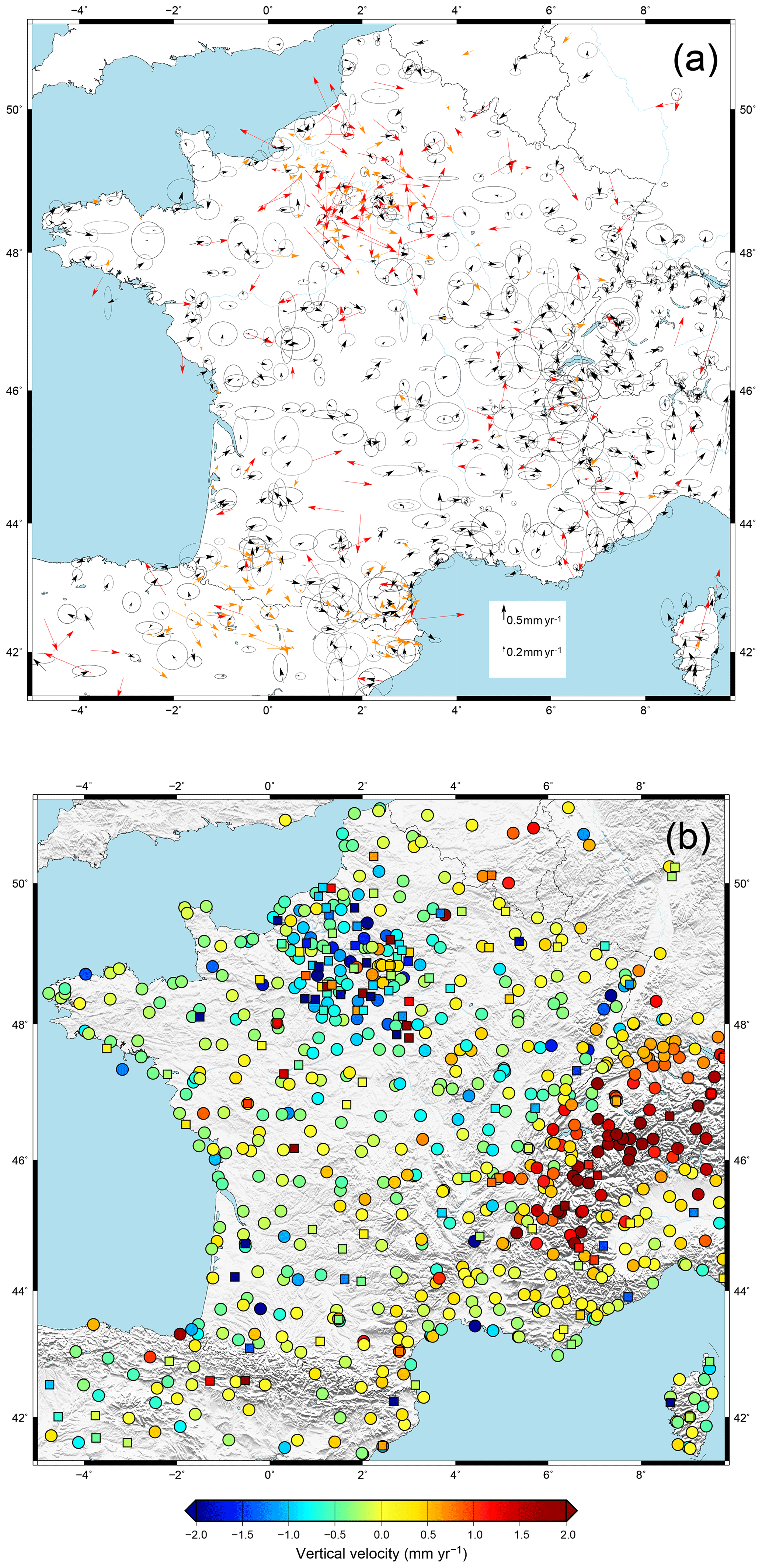
Figure 3(a) Horizontal velocities for permanent and campaign stations in France-centered reference frame. Black indicates the horizontal velocities associated with their 95 % uncertainties, orange the horizontal velocities whose uncertainty is larger than 0.3 mm yr−1 for which the uncertainties are not represented for graphic reasons, and red the horizontal velocities of the stations identified as outliers and (b) vertical velocities; the squares correspond to the outliers, whose identification was made from the horizontal components.
In our local France-centered reference frame, individual station velocities and uncertainties tend to be of the same order of magnitude (Fig. 3), precluding a detailed interpretation of the kinematics and deformation. We use two independent statistical approaches (clustering and spatial smoothing) to extract spatially coherent information on the present-day deformation at a spatial scale of 100–200 km. To a first order, this distance represents the expected scale of tectonic deformation in France and neighboring regions. It corresponds to the average width of the major tectonic systems (French Alps, Pyrenees, South Armorican Shear Zone, etc.). We apply each method (clustering and smoothing) to the GPS velocities. The two methods are fully independent. Clustering only provides a velocity field and no strain rate field. The strain rate map (Fig. 7a) is computed using the smoothing method only (based on the GPS velocities), independently of the clustering analysis.
The smoothing and clustering methods are tuned to extract coherent signals on geographical domains at this spatial scale by minimizing local noise without losing the regional signal. The robustness of the results is estimated with two independent approaches:
-
We use synthetic data to estimate each method detection level. The synthetic dataset corresponds to random velocities derived from the combination of a null long-term velocity, annual and semiannual sinusoids, position offsets and colored noise (Eq. 1), with all parameters based on our GPS data characteristics (see Masson et al., 2019a, for details). Thus, this dataset corresponds to null velocity and strain rate fields with additional noise representative of our actual GPS data. Synthetic and actual data are compared after processing by the clustering or smoothing methods to estimate their respective detection levels.
-
We estimate statistical standard errors on the velocities and strain rates calculated with the clustering or smoothing methods using a simple Monte Carlo and bootstrap resampling of the original GPS velocities on the basis of their standard errors (Monte Carlo) and regional distribution (bootstrap). Hereafter, the smoothed or clustered velocities and strain rates are given as the mean and 95 % confidence interval (CI95) of the Monte Carlo or bootstrap samples. Using 95 % confidence intervals (rather than the more common standard errors) yields a strict definition of significant vs. not significant signals, which should be nuanced in cases of values close to the limits.
3.1 Clustering applied to GPS velocities
Clustering is a parametric unsupervised learning method and has been used in GNSS analyses to perform geographical groupings of stations with optimum velocity consistency (Savage et al., 2013, 2018; Liu et al., 2015; Özdemir et al., 2019). Several methods of clustering exist; here we use the k-means method (Hartigan and Wong, 1979), whose advantage is that the formed groups do not have a predefined geometry or size and allow for abrupt changes so as to adapt to local geometries. In order to extract spatial coherence in the velocity field, we define clusters using station coordinates (longitude and latitude) and horizontal (north and east) or vertical velocities; vertical velocities are treated independently because of their large dispersions and uncertainties. The variables are not normalized, in order to ensure first-order geographical clustering with secondary adjustments based on the velocity variability.
The analysis takes place in four steps: (1) choice of random clusters (based on a predefined initial number); (2) minimization of the Euclidian distances between the cluster centroids and the different observations; (3) shift of the initial centroids to the mean of the groups; (4) minimization of the Euclidian distances according to new centroids from an increase in the cluster number and modifications of their boundaries. The last three steps are repeated until convergence to the predefined final number of clusters and no observation changes clusters. At the end of the process, each GNSS station is attributed a velocity that corresponds to its final cluster median.
We run the algorithm 50 000 times in order to take into account the following three stochastic aspects of the computation.
-
The choice of the final number of clusters is crucial as it controls the average cluster size (geographical extent and number of stations). In order to average velocities over a 100–200 km spatial scale, we vary the final number of clusters between 75 and 200 (uniform distribution), resulting in a mean cluster area of 27.5×10³ km2 (i.e., scale of ca. 166 km), with variations of a factor of 2–3 in the cluster sizes. A larger number of clusters (smaller spatial scale) leads to strong variability and incoherence of the final velocities.
-
The random choice of initial clusters results in variability in the final results. We take advantage of this effect to improve the statistics of the results by varying the initial number of clusters between 1 and the final number divided by 2 (uniform distribution).
-
In order to account for each station-specific velocity uncertainty, we redefine its velocity using a random draw in a normal distribution defined by its velocity mean and standard deviation. Thus, sites with high uncertainties have a large variability and less weight in the overall cluster analysis.
For each station, the final velocity is defined as the median, with the associated 95 % confidence interval, of the 50 000 computations. The clustered horizontal and vertical velocities are presented in Figs. 4 and 5a. The comparison of clustered velocities based on the actual GPS data and on the synthetic dataset indicates a detection level for the horizontal velocities of 0.12 mm yr−1 (see Fig. S3.1). Only 10 % of the stations is associated with a clustered velocity below this detection level (Fig. 4a). Vertical velocities are not analyzed with the synthetic comparison because of their high dispersion and spatial noise. Their interpretation is thus subject to caution.

Figure 4(a) Horizontal velocities from clustering with (b) 95 % confidence interval (CI95). In brown: horizontal velocities below the detection level based on the synthetic dataset.
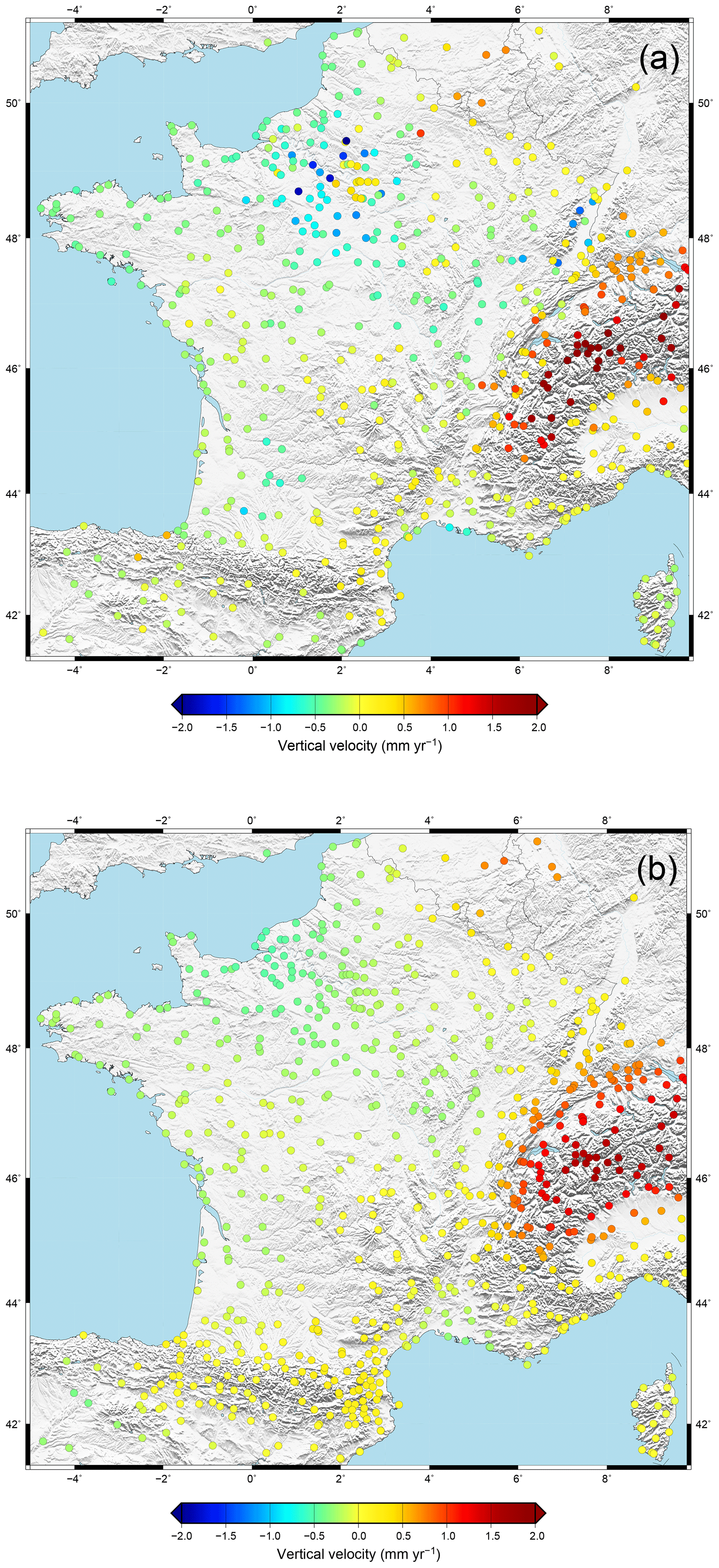
Figure 5Vertical velocities (a) from clustering and (b) from Gaussian smoothing.
Coherent horizontal patterns are observed with velocities of ca. 0.1–0.4 mm yr−1 (Fig. 4a). Associated 95 % confidence intervals are mostly ca. 0.1–0.2 mm yr−1, except in the Pyrenees, Alps and Paris Basin, where they reach 0.4–0.5 mm yr−1 (Fig. 4b). The vertical velocities are associated with a larger CI95 of ca. 0.4–0.8 mm yr−1. The only significant vertical patterns (Fig. 5a) are the subsidence in the Paris Basin (ca. 0.5–1 mm yr−1) and uplift in the Western and Central Alps (ca. 0.5–2 mm yr−1).
3.2 Gaussian smoothing applied to GPS velocities
Smoothing is a standard technique for data interpolation, filtering and noise reduction. It allows the extraction of a continuous field, minimizing small-scale noise and precluding abrupt spatial changes. We use a Gaussian smoothing function to compute at any point in space a smoothed velocity Vg based on all GPS velocities weighted according to their standard errors and their distance to the computation point (after Mazzotti et al., 2011):
with
where i is the velocity component (North, East or Up), rg is the smoothing length (half-width of the Gaussian function), Vn and σn are the velocity and standard error of the GPS station n, and Δn is the distance to the GPS station n. The spatial derivative of the Gaussian function can be used to compute the smoothed horizontal strain rate tensor at the same location:
where i and j are the velocity component (North, East or Up) and Δn(i,j) is the distance to the GPS station n in the east or north direction.
The smoothing length rg controls the correlation length of the computed velocity and strain rate fields. To first order, this correlation length can be associated with the Gaussian smoothing scale , which corresponds to the distance within which the GNSS stations contribute 67 % of the computed velocity (95 % contribution within 2Dg). In order to extract deformation signals at the 100–200 km scale with minimum contribution from local noise, we estimate an optimal smoothing scale on the basis of a series of tests on the synthetic velocity data. Smoothing scales Dg≤120–140 km result in smoothed velocities that can reach up to 0.1–0.2 mm yr−1 (compared to the true null velocity), whereas scales Dg > 140 km are associated with smoothed velocities smaller than 0.1 mm yr−1 (see Fig. S4). Hereafter, we present results based on the smoothing scale Dg=160 km, keeping in mind that results with 140 > Dg > 200 km are similar to or better than 0.1 mm yr−1.
The smoothed velocity and horizontal strain rate fields, and associated 95 % confidence intervals, are presented in Figs. 5b, 6 and 7 (the smoothed horizontal strain rate fields but with outliers is presented in Fig. S5). Horizontal strain rates are expressed in terms of “maximum strain rate”:
where e1 and e2 are the principal components of the strain rate tensor. The comparison of the smoothed velocities and strain rates based on the actual GPS data with those based on the synthetic dataset (see Figs. S3.2 and S3.3) indicates detection levels of 0.04 mm yr−1 for the horizontal velocities and yr−1 for the horizontal strain rates. Less than 5 % of the results are below the detection level (Figs. 6a and 7a), similar to the clustering analysis.
Coherent patterns are observed with horizontal (or vertical) velocities of ca. 0.1–0.4 mm yr−1 (0.2–1.6 mm yr−1), similar to a first order to those obtained with the clustering method (Fig. 4 vs. Figs. 6 and 5). Statistical 95 % confidence intervals on the horizontal velocities and strain rates are, respectively, ca. 0.05–0.1 mm yr−1 and ca. 0.7– yr−1, indicating that more than two-thirds of the velocities and strain rates are statistically significant (Figs. 6 and 7).
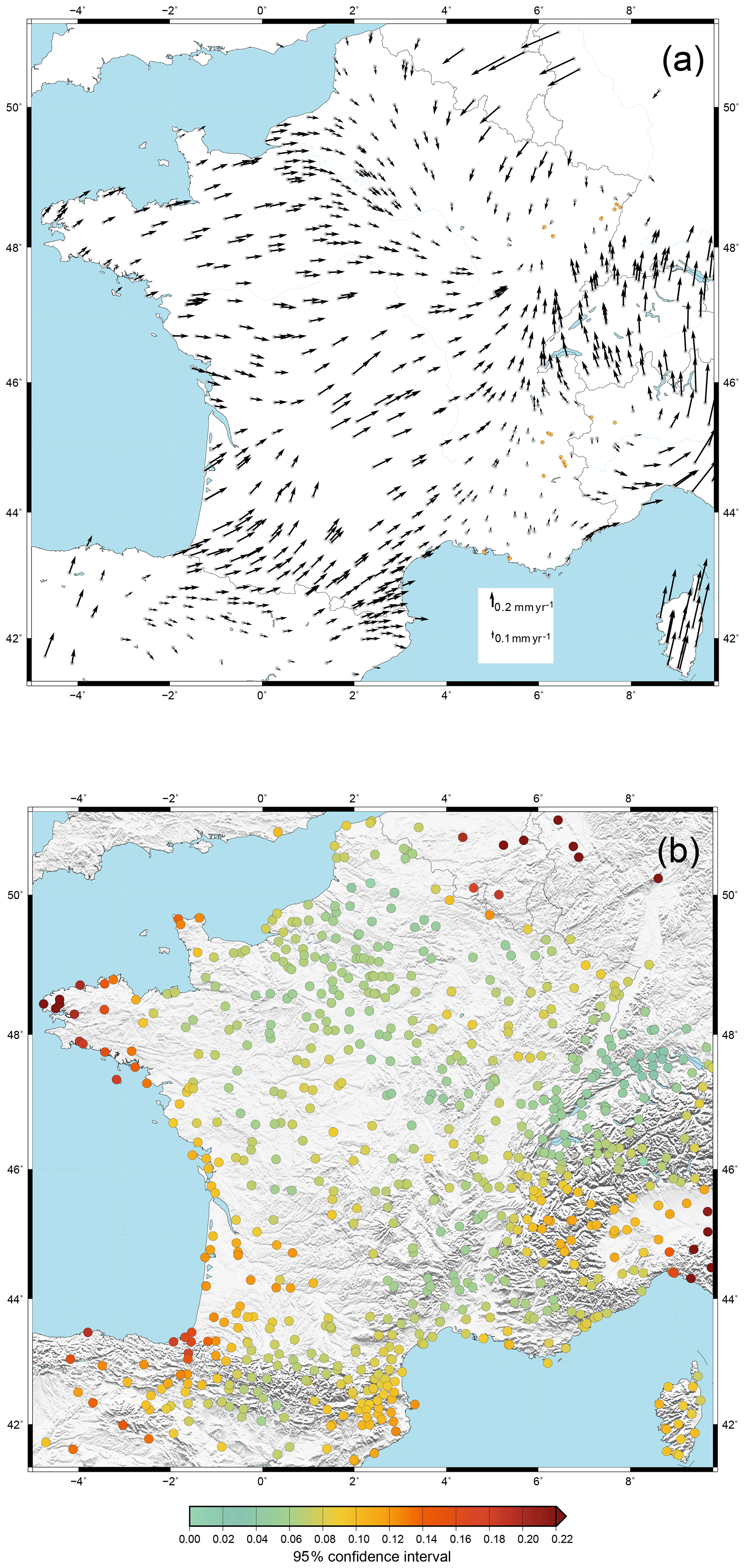
Figure 6(a) Horizontal velocities for each site from Gaussian smoothing with (b) 95 % confidence interval (CI95). In brown: horizontal velocities below the detection level based on the synthetic dataset.

Figure 7(a) Smoothed horizontal strain rate field with a grid of 0.1∘ (strain rate tensors are plotted every 0.5∘) and (b) associated 95 % confidence interval (CI95).
3.3 Coherence of clustering and Gaussian smoothing results
To first order, the clustered and smoothed velocity fields show a striking agreement in both the horizontal components (Figs. 4a and 6a) and the vertical components (Fig. 5). In order to better characterize the coherence of the two velocity fields, and its potential regional variability, we compute the difference between the two methods for each velocity component (North, East and Up). The dispersion of the North and East differences (see Fig. S6) illustrates the consistency of the two methods: 28 % of the differences are smaller than 0.05 mm yr−1 and 60 % are smaller than 0.10 mm yr−1. In Fig. 8, we identify the areas where the horizontal velocity differences are larger than 0.1 mm yr−1: the westernmost part of Brittany, parts of the Paris Basin, most of the Western Alps (especially near the France–Switzerland–Italy borders), and the Pyrenees and their northern foreland. For these areas, the interpretations of the velocity fields must be carried out with caution. These velocity differences at the level of 0.1–0.3 mm yr−1 can be related to either abrupt spatial variations in the actual velocity and deformation patterns or biases and limitations in one or both methods. Figure S7 shows vector differences between the two methods and the differences between the two velocity fields and the GPS velocities and confirms what is shown on Fig. 8.
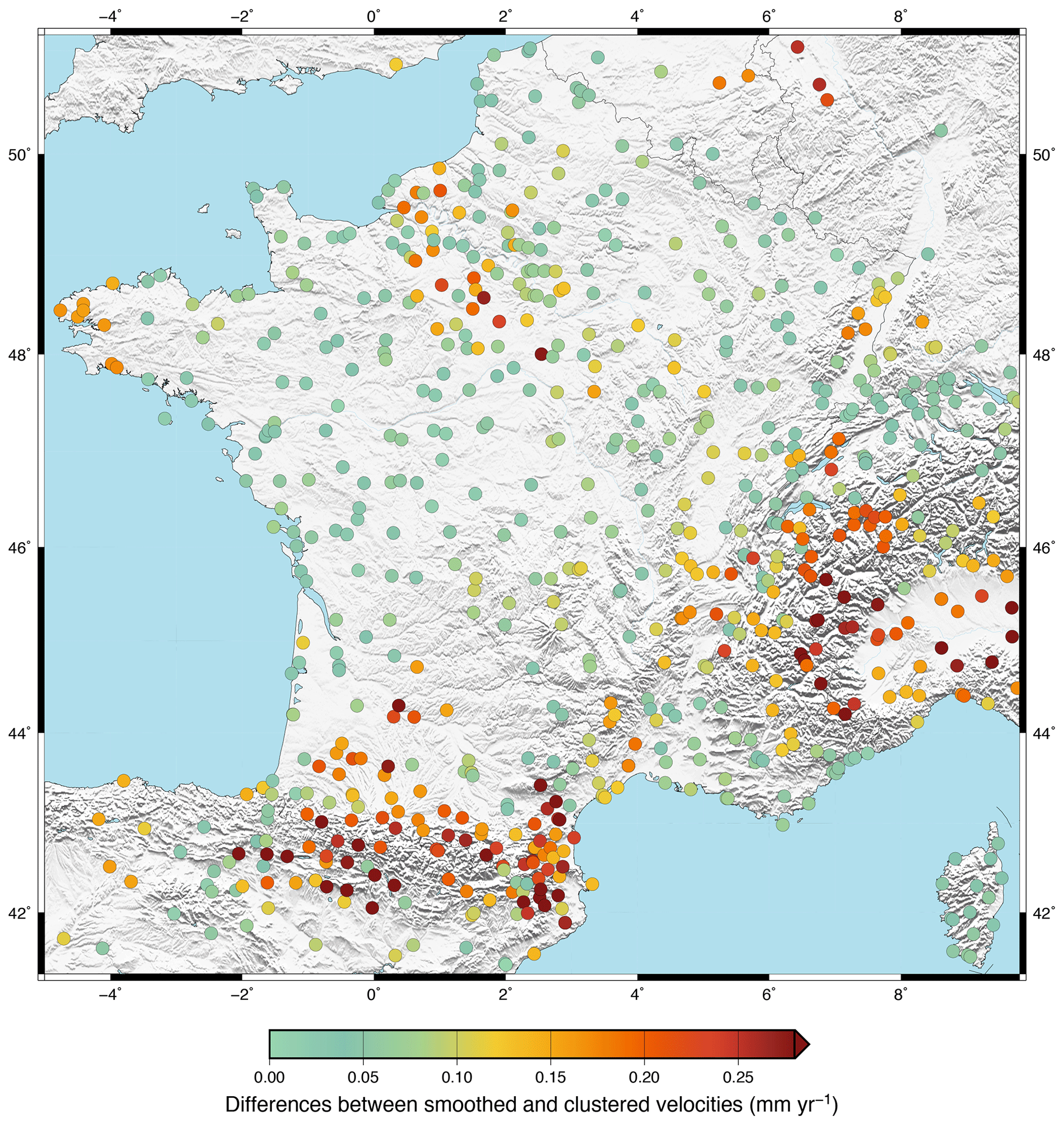
Figure 8Map of the differences between the velocities obtained from the clustering and from the Gaussian smoothing methods.
The analysis of the deformation in France and conterminous regions can be guided using the uncertainty levels described in Sect. 3. To a first order, we consider as “well resolved” areas of a 100–200 km scale or more within which (1) the GNSS station density is similar to or larger than the network average and (2) the clustered and smoothed velocities are consistent at 0.1 mm yr−1 or better. In contrast, areas where one of the criteria is not satisfied are considered less well constrained. These correspond roughly to the region northeast of the France–Belgium–Germany border (very low station density), the center and northwest of the Paris Basin, most of the Alps and northwestern Italy, and the Spain–Pyrenees region south of about 44∘ N (Fig. 8). The last three are discussed in more detail in Sect. 5.
Most of central, northern and western France is associated with coherent clustered and smoothed velocities resolved at ca. 0.1 mm yr−1. There, the first-order and most important deformation signal is that, relative to the France-centered reference, western and central France are characterized by eastward to northeastward motions of 0.1–0.2 mm yr−1, whereas northeastern France shows 0–0.2 mm yr−1 southward to southwestward velocities (Figs. 4 and 6). The resulting overall deformation pattern corresponds to a belt of N–S to NE–SW shortening of (1–2) yr−1 in central and eastern France (Fig. 7).
In detail, this first-order kinematic pattern is associated with regional variability, with extension into the Armorican Massif and a complex strain rate pattern in the Aquitaine Basin. In more detail, from west to east, the following can be observed:
-
The western Armorican Massif is associated with a small E–W extension rate (0.4– yr−1, CI95=1.0– yr−1) subject to caution because of the high uncertainty. The smoothed and clustered velocities differ, likely due to the network configuration (lack of stations on three sides of the peninsula), precluding a more detailed spatial analysis. In the eastern part, the extension rotates to a N–S direction with similar rates and slightly lower uncertainties (0.3– yr−1, CI95=0.6– yr−1). Smoothed and clustered vertical velocities reveal a low generalized subsidence (−0.2 mm yr−1, CI95≈0.1 mm yr−1 and −0.3 mm yr−1, CI95≈0.3 mm yr−1, respectively). The overall extension is roughly compatible with the deformation and stress analyses from focal mechanisms that indicate NE–SW extension in Brittany (Mazabraud et al., 2004).
-
To the south, the Aquitaine Basin shows a complex pattern of high strain rates (1.5– yr−1) with N–S shortening in the northwest, E–W shortening in the southwest in the Pyrenees foreland and E–W extension in the east at the border with the Massif Central (Fig. 7). All rates are statistically significant, but the low density of GNSS stations in the east strongly limits the validity of the E–W extension pattern. Both smoothed and clustered vertical velocities show a barely significant small subsidence (−0.15 mm yr−1, CI95≈0.1 mm yr−1 and −0.3 mm yr−1, CI95≈0.4 mm yr−1, respectively). The strong and spatially varying strain rates are surprising in light of the low seismicity (Fig. 1) and very few indications of active tectonics (Baize et al., 2013; Jomard et al., 2017). Peculiar hydrological loading is not reflected in the time series annual or pluri-annual signals.
-
To the east, the large-scale pattern of E–W to NE–SW shortening is observed in the Massif Central (0.8– yr−1, CI95=0.5– yr−1), associated with near-zero vertical velocities, and in northeastern France, including strong shortening rates (2– yr−1) rotating from E–W in the Bresse to N–S in the Upper Rhine Graben (Fig. 7). There, clustered velocities show a small subsidence (−0.4 mm yr−1, CI95≈0.6 mm yr−1) not present in the smoothed velocities, indicating either a small-scale signal (< 10 s km) or noise in the original data. This deformation pattern is discussed in more detail in Sect. 5.3.
Finally, Corsica presents a coherent, near-rigid northward motion relative to the continent, similar between the smoothing and clustering methods at 0.4 mm yr−1 (CI95≈0.1 mm yr−1), that may be related to the present-day tectonics of the Apennine–Tyrrhenian system (Figs. 4 and 6). This northern motion creates a domain of significant NNW–SSE shortening of yr−1 (CI yr−1) north of Corsica (Fig. 7), compatible with the tectonic and seismicity observations along the Ligure Margin (Larroque et al., 2012, 2016).
Complex velocity and deformation patterns require more careful analysis in three specific regions: the Paris Basin, the Pyrenees and the Western Alps (associated with the Upper Rhine Graben). The first is associated with a very low seismicity, unlike the other two that are the most seismically active area of western Europe.
5.1 The Paris Basin
For 20 % of the stations in the Paris Basin, the differences between the clustered and smoothed velocities are between 0.1 and 0.3 mm yr−1 (Fig. 8), but there is a general consistency in the spatial variations in the velocity directions: from west to east, the direction is ENE to SE for smoothing (Fig. 6a) and NE to SSE for clustering (Fig. 4a). The spatial variations are by definition sharper for the clustering results. These result in a significant NE–SW shortening ( yr−1, CI yr−1), part of the large-scale shortening belt (Sect. 4), without seismicity and with very few identified active faults (Fig. 1). Smoothed and clustered vertical velocities show a generalized subsidence (−0.3 mm yr−1, CI95≈0.1 mm yr−1 and −0.5 mm yr−1, CI95≈0.7 mm yr−1, respectively) with, however, a potential small area of uplift around Paris for the clustered velocities (0.35 mm yr−1, CI95≈0.6 mm yr−1). The amplitudes of seasonal signals are more important than the national median (+29 % for the annual signals in E and +48 % in U) suggesting that hydrological processes or natural resource extraction may contribute to the observed deformation.
5.2 Pyrenees
Most of the GNSS sites in the Pyrenees are campaign sites with large uncertainties. For about 50 % of the stations, the differences between the smoothed and clustered velocities are between 0.1 and 0.4 mm yr−1, but the orientations are similar (Figs. 4a and 6a). These differences may be due to the fact that most of the sites were surveyed only twice, with the first survey in the mid 1990s, when the satellite orbits and clocks were of lower quality and the permanent GPS network was very sparse providing only few common stations for the solution combination (see Sect. 2.4.2). As a result, the campaign velocities are associated with large standard errors, leading to a low weight in the smoothing results.
Despite these differences, a first-order pattern of N–S extension is clearly visible in both the clustered and smoothed velocities (between 0.2 and 0.4 mm yr−1). The extension rate decreases from west ( yr−1, CI yr−1) to east ( yr−1, CI yr−1), with an associated rotation of the extension direction from NNE–SSW to N–S (Fig. 9). Most vertical velocities are not significant, except in the eastern region with a value barely significant of 0.18 mm yr−1, CI95≈0.2 mm yr−1 for the smoothed velocities.
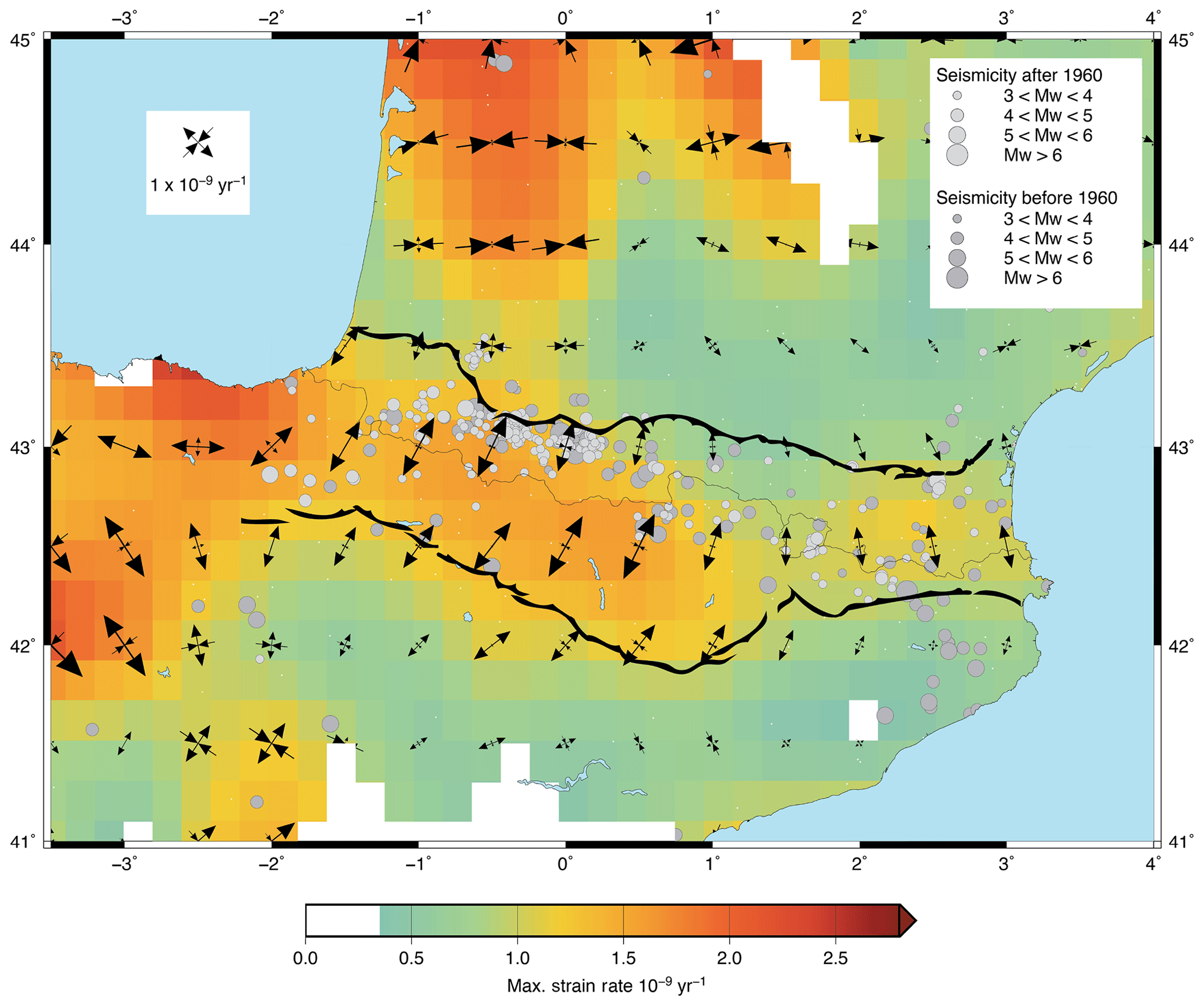
Figure 9Smoothed horizontal strain rate field for Pyrenean permanent and campaign stations, with instrumental (dark gray) and historical (light gray) seismicity (SHARE and SI-Hex) and the main fault zones bordering the Pyrenees to the south and to the north.
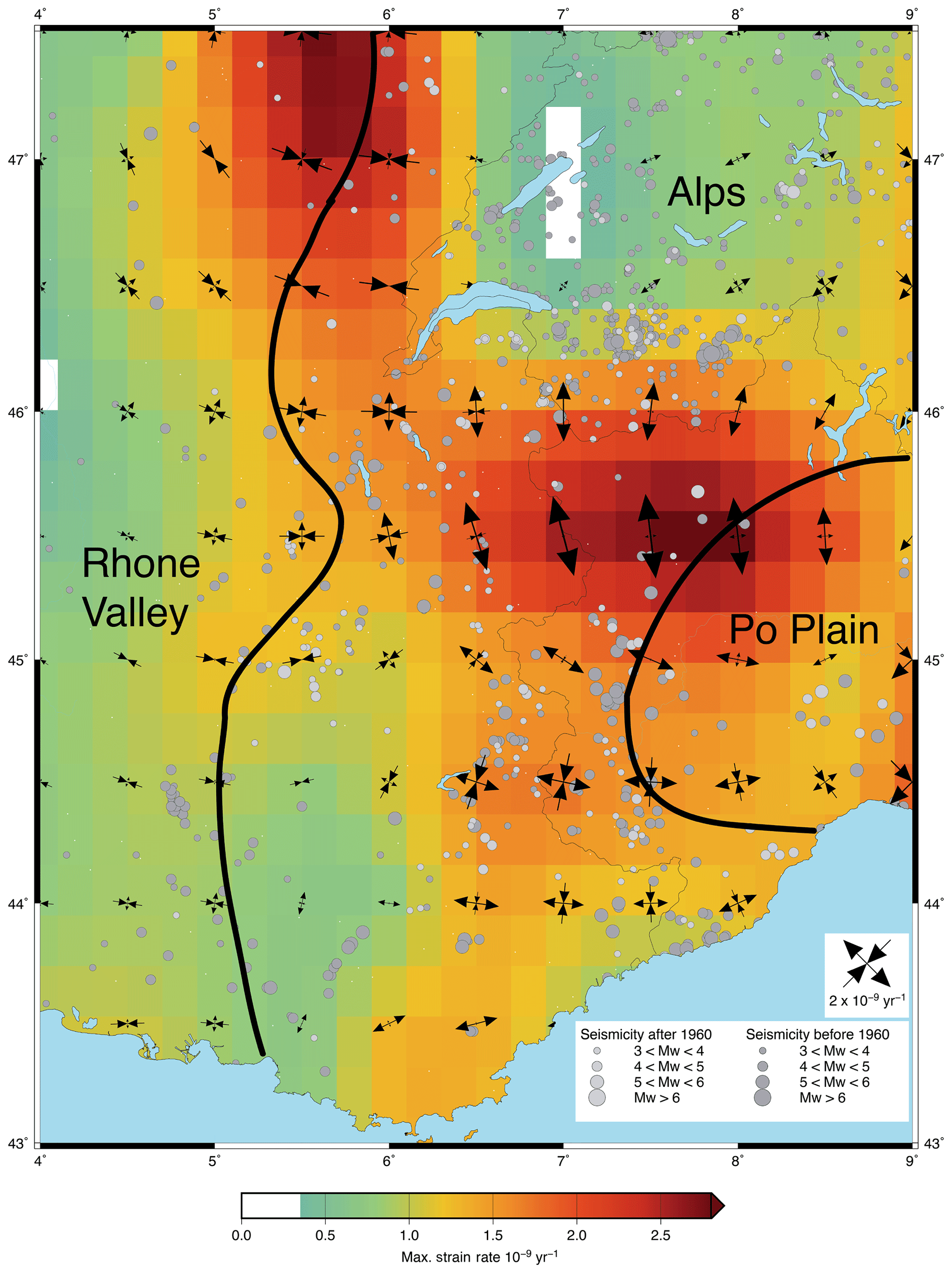
Figure 10Smoothed horizontal strain rate field for Alpine permanent and campaign stations, with instrumental (dark gray) and historical (light gray) seismicity (SHARE and SI-Hex) and the limits between Alps and Po Plain and Rhône Valley.
The seismicity of the Pyrenees is heterogeneously distributed along the orogen (Chevrot et al., 2011; Calvet et al., 2013). It is diffuse in the east and more focused in the west along the North Pyrenean Fault system (Fig. 9). In the central part of Pyrenees, the GPS-based extension zone extends over a wider area than the seismicity but remains located within the northern and southern limits of the Pyrenean orogen. This difference in the spatial distribution of the seismicity, orogen topography and GPS extension may be attributed to three potential causes.
-
Actual present-day deformation only takes place within the zone of high seismicity, and our GPS analysis does not allow such a fine localization because of the limits in the smoothing and cluster spatial scales (100–200 km, see Sect. 3).
-
The location of the current seismicity does not reflect the location of the deformation on a longer timescale, which is, in contrast, captured by GPS data. This would indicate potential large earthquakes outside the present-day seismicity zone.
-
The deformation measured by GPS at the surface reflects a deeper aseismic deformation centered on the orogen center or highest topography and not only on the crustal seismic deformation.
5.3 The Alps and the Upper Rhine Graben
In the Alps, for 28 % of the stations the differences between the clustering and smoothing methods are between 0.1 and 0.5 mm yr−1, but the velocities have consistent directions. Roughly northward velocities of 0.2–0.4 mm yr−1 in the Swiss Alps and nearby Jura (Figs. 4a and 6a) result in a significant N–S extension of ca. yr−1 near and south of the Switzerland–Italy border, and N–S shortening of ca. yr−1 in the Vosges–Upper Rhine Graben–Black Forest region. The region in between (most of Switzerland) is associated with low deformation (Fig. 7). The western foreland of the Alps (Saône Valley, the Jura and Rhône Valley) is mainly characterized by E–W shortening (ca. 0.8– yr−1), associated with the eastward motion of the Massif Central and central France (see Sect. 4). These results are consistent with those reported in other geodetic studies (Sanchez et al., 2018). The central and southern parts of the Western Alps show a transition from N–S extension to strike-slip and E–W extension in the south, associated with the 0.2–0.4 mm yr−1 eastward motion in southeasternmost France and the western Po Plain (Figs. 4a and 6a). To a first order, these deformation patterns in the French Alps are consistent with those observed in Walpersdorf et al. (2018), although our strain rate amplitudes are on average 2–3 times smaller, potentially due to the lower number of stations and spatial coverage used in Walpersdorf et al. (2018).
The vertical velocities (Fig. 5) have the same large-scale pattern in the two methods, with a maximum of uplift in the northern French and Swiss Alps (ca. 1.5–2 mm yr−1) decreasing to near-zero (±0.5 mm yr−1) in the Southern Alps, the Rhône Valley, the Po Plain and the Jura. This pattern is consistent with that derived from previous GPS data analysis and combinations with leveling data (Nocquet et al., 2016; Sternai et al., 2018). A more detailed analysis of the transition from relatively fast uplift to near-zero (or small subsidence) rates is restricted by the limits of the smoothing and clustering methods, as well as the low precision of individual stations.
The seismicity is distributed over the whole Alpine system (Figs. 1 and 10), with a concentration of epicenters in the southwest of Switzerland (Deichmann et al., 2012). For the regions of the Vosges and Jura, the analysis of focal mechanisms provides results compatible with our geodetic deformations (Plenefisch et al. al., 1997; Maurer et al., 1997; Sue et al., 1999, 2007). The compatibility suggests a tectonic origin of this deformation. The GPS-derived N–S extension near the Swiss–Italian–French borders is compatible with the earthquake focal mechanism analysis of Delacou et al. (2004), but the peak of deformation is located south of the seismicity concentration in a region of relatively low activity (Fig. 10). The location of the maximal extension depends on how the uncertainties from the Swiss velocity field are scaled when combined with our solution. If the weight of the Swiss velocities is reduced, the maximum extension is shifted 50 km northward, near the Switzerland–Italy border at a location consistent with the seismicity. This issue points out the importance of consistent processing and uncertainty analysis of all RINEX. In addition, the region of Aosta is devoid of stations in our analysis, leading to an additional source of uncertainty regarding the precise localization of the maximum deformation. If the GPS–seismicity localization difference proves to be real, it may the expression of deformation not only accommodated by seismicity or of a lack of large earthquakes in the high strain rate area.
The application of semiautomatic statistical methods allows us to evaluate the potential of dense networks and large GNSS datasets to extract spatially coherent and significant deformation rates in France and conterminous western European countries. In particular, the combination of spatial smoothing and clustering approaches more than 900 GPS velocities results, for the first time, in the definition of horizontal velocity and strain rate fields with a 95 % confidence level of ca. 0.1–0.2 mm yr−1 (ca. 0.5– yr−1) on spatial scales of 100–200 km or more (Figs. 4b, 6b, 7b). In most of the study area, the calculated velocity and strain rate patterns are just at or above the 95 % significant level. Based on this analysis, several conclusions can be drawn.
-
The first-order and most important deformation signal in France and neighboring western European countries is a belt of N–S to NE–SW shortening of ca. 0.2–0.4 mm yr−1 (1– yr−1) in central and eastern France.
-
We observe orogen-normal (radial) extension of ca. 1– yr−1 in the Western Alps and the Pyrenees, associated with radial shortening in the Western Alps foreland, compatible with previous studies (e.g., Rigo et al., 2015; Walpersdorf et al., 2018).
-
In addition, several areas (Aquitaine Basin, Brittany, Bresse) present unexpectedly high deformation rates, some of them anticorrelated with the local level of seismicity.
-
The only significant vertical velocity patterns are the subsidence in the Paris Basin (ca. 0.5–1 mm yr−1) and uplift in the Western and Central Alps (ca. 0.5–2 mm yr−1).
These results open questions about the origin and the timescales of these deformations, as well as their relationship with seismicity and the potential for significant aseismic deformation in France and western Europe. In particular, these small velocity and deformation signals may relate to a variety of non-tectonic forces, such as glacial isostatic adjustment or hydrological loading, operating from a local (100–200 km) to a continental scale. In North America, Kreemer et al. (2018) have shown that, to first order, geodetic deformation is not directly correlated to seismicity and that the link between long-term tectonic processes, transient processes (GIA, glacial isostatic adjustment), seismicity and geodetic deformation is not simple at the scale of the regional deformation (> 100 km).
In addition to these observations, our methodological developments highlight two conclusions regarding the potential of future more detailed analyses:
-
The station density is critical to eliminate outliers and extract spatially coherent deformation signals in very low-deformation areas such as intraplate domains and volcanic areas. Non-geodetic networks and campaign data, although of potentially lower resolution compared to permanent geodetic stations, can provide important densification.
-
A consistent processing of the RINEX and position time series is essential to extract significant deformation. Our results for the western Alps are currently limited by the post-processing combination of velocity solutions that result in uncertainties of ca. 50 km in the peak of the extension pattern.
Finally, the combination of mathematical techniques for extracting spatially coherent signals can provide confidence, or point out limitations, in the observed deformation patterns beyond the application of simple standard error estimations.
The data_providers file shows all the sources used to obtain the data present in this study, and the velocities file contains the velocities used in this study (https://doi.org/10.15148/2cdc72ec-1066-486c-aef7-9da36662f46d, Masson et al., 2019b). The time series analyses were performed using R (R Core Team, 2016). Maps were done with GMT5 (Wessel et al., 2011).
The supplement related to this article is available online at: https://doi.org/10.5194/se-10-1905-2019-supplement.
CM, ED and PV processed the GPS data. CM and SM developed the analysis methods. CM did the statistical analyses. CM, SM and PV interpreted the results and wrote the article.
The authors declare that they have no conflict of interest.
We are grateful to the technical teams of Montpellier and RENAG-RESIF. We deeply thank all data providers.
This paper was edited by Simon McClusky and reviewed by Mimmo Palano and one anonymous referee.
Altamimi, Z., Rebischung, P., Métivier, L., and Collilieux, X.: ITRF2014: A new release of the International Terrestrial Reference Frame modeling nonlinear station motions, J. Geophys. Res.-Sol. Ea., 121, 6109–6131, https://doi.org/10.1002/2016JB013098, 2016.
Baize, S., Cushing, E. M., Lemeille, F., and Jomard, H.: Updated seismotectonic zoning scheme of Metropolitan France, with reference to geologic and seismotectonic data, B. Soc. Geol. Fr., 184, 225–259, https://doi.org/10.2113/gssgfbull.184.3.225, 2013.
Banerjee, P., Bürgmann, R., Nagarajan, B., and Apel, E.: Intraplate deformation of the Indian subcontinent, Geophys. Res. Lett., 35, L18301, https://doi.org/10.1029/2008GL035468, 2008.
Battaglia, M., Murray, M. H., Serpelloni, E., and Bürgmann, R.: The Adriatic region: An independent microplate within the Africa-Eurasia collision zone, Geophys. Res. Lett., 31, L09605, https://doi.org/10.1029/2004GL019723, 2004.
Beavan, J., Wallace, L. M., Palmer, N., Denys, P., Ellis, S., Fournier, N., Hreinsdottir, S., Pearson, C., and Denham, M.: New Zealand GPS velocity field: 1995–2013, New Zeal. J. Geol. Geop., 59, 5–14, https://doi.org/10.1080/00288306.2015.1112817, 2016.
Boehm, J., Werl, B., and Schuh, H.: Troposphere mapping functions for GPS and very long baseline interferometry from European Centre for Medium-Range Weather Forecasts operational analysis data: TROPOSPHERE MAPPING FUNCTIONS FROM ECMWF, J. Geophys. Res.-Sol. Ea., 111, B02406, https://doi.org/10.1029/2005JB003629, 2006.
Breiman, L., Friedman, J., Stone, C. J., and Olshen, R. A.: Classification and regression trees, CRC Press, Chapman and Hall, Wadsworth, New York, 251–257, 1984.
Brockmann, E., Ineichen, D., Marti, U., Schaer, S., Schlatter, A., and Villiger, A.: Determination of Tectonic Movements in the Swiss Alps Using GNSS and Levelling, in: Geodesy for Planet Earth, Vol. 136, edited by: Kenyon, S., Pacino, M. C., and Marti, U., Springer Berlin Heidelberg, Berlin, Heidelberg, 689–695, 2012.
Calais, E. and Stein, S.: Time-Variable Deformation in the New Madrid Seismic Zone, Science, 323, 1442–1442, https://doi.org/10.1126/science.1168122, 2009.
Calvet, M., Sylvander, M., Margerin, L., and Villaseñor, A.: Spatial variations of seismic attenuation and heterogeneity in the Pyrenees: Coda Q and peak delay time analysis, Tectonophysics, 608, 428–439, https://doi.org/10.1016/j.tecto.2013.08.045, 2013.
Cara, M., Cansi, Y., Schlupp, A., Arroucau, P., Béthoux, N., Beucler, E., Bruno, S., Calvet, M., Chevrot, S., Deboissy, A., Delouis, B., Denieul, M., Deschamps, A., Doubre, C., Fréchet, J., Godey, S., Golle, O., Grunberg, M., Guilbert, J., Haugmard, M., Jenatton, L., Lambotte, S., Leobal, D., Maron, C., Mendel, V., Merrer, S., Macquet, M., Mignan, A., Mocquet, A., Nicolas, M., Perrot, J., Potin, B., Sanchez, O., Santoire, J.-P., Sèbe, O., Sylvander, M., Thouvenot, F., Van Der Woerd, J., and Van Der Woerd, K.: SI-Hex: a new catalogue of instrumental seismicity for metropolitan France, B. Soc. Geol. Fr., 186, 3–19, https://doi.org/10.2113/gssgfbull.186.1.3, 2015.
Carafa, M. M. C. and Bird, P.: Improving deformation models by discounting transient signals in geodetic data: 2. Geodetic data, stress directions, and long-term strain rates in Italy: Discounting Transient Signals: 2. Italy, J. Geophys. Res.-Sol. Ea., 121, 5557–5575, https://doi.org/10.1002/2016JB013038, 2016.
Cardozo, N. and Allmendinger, R. W.: SSPX: A program to compute strain from displacement/velocity data, Comput. Geosci., 35, 1343–1357, https://doi.org/10.1016/j.cageo.2008.05.008, 2009.
Chevrot, S., Sylvander, M., and Delouis, B.: A preliminary catalog of moment tensors for the Pyrenees, Tectonophysics, 510, 239–251, https://doi.org/10.1016/j.tecto.2011.07.011, 2011.
Chousianitis, K., Ganas, A., and Evangelidis, C. P.: Strain and rotation rate patterns of mainland Greece from continuous GPS data and comparison between seismic and geodetic moment release: Kinematics Of Mainland Greece, J. Geophys. Res.-Sol. Ea., 120, 3909–3931, https://doi.org/10.1002/2014JB011762, 2015.
Deichmann, N., Clinton, J., Husen, S., Edwards, B., Haslinger, F., Fäh, D., Giardini, D., Kästli, P., Kradolfer, U., and Wiemer, S.: Earthquakes in Switzerland and surrounding regions during 2011, Swiss J. Geosci., 105, 463–476, https://doi.org/10.1007/s00015-012-0116-2, 2012.
Delacou, B., Sue, C., Champagnac, J.-D., and Burkhard, M.: Present-day geodynamics in the bend of the western and central Alps as constrained by earthquake analysis, Geophys. J. Int., 158, 753–774, https://doi.org/10.1111/j.1365-246X.2004.02320.x, 2004.
Dow, J. M., Neilan, R. E., and Rizos, C.: The International GNSS Service in a changing landscape of Global Navigation Satellite Systems, J. Geodesy, 83, 191–198, https://doi.org/10.1007/s00190-008-0300-3, 2009.
Farolfi, G. and Del Ventisette, C.: Contemporary crustal velocity field in Alpine Mediterranean area of Italy from new geodetic data, GPS Solutions, 20, 715–722, https://doi.org/10.1007/s10291-015-0481-1, 2016.
Gazeaux, J., Williams, S., King, M., Bos, M., Dach, R., Deo, M., Moore, A. W., Ostini, L., Petrie, E., Roggero, M., Teferle, F. N., Olivares, G., and Webb, F. H.: Detecting offsets in GPS time series: First results from the detection of offsets in GPS experiment: Detecting Offsets In Gps Time Serie, J. Geophys. Res.-Sol. Ea., 118, 2397–2407, https://doi.org/10.1002/jgrb.50152, 2013.
Griffiths, J.: Combined orbits and clocks from IGS second reprocessing, J. Geodesy, 93, 177–195, https://doi.org/10.1007/s00190-018-1149-8, 2019.
Gunawan, E. and Widiyantoro, S.: Active tectonic deformation in Java, Indonesia inferred from a GPS-derived strain rate, J. Geodynam., 123, 49–54, https://doi.org/10.1016/j.jog.2019.01.004, 2019.
Hartigan, J. A. and Wong, M. A.: Algorithm AS 136: A K-Means Clustering Algorithm, J. R. Stat. Soc. C-Appl., 28, 100–108, 1979.
Héroux, P. and Kouba, J.: GPS Precise Point Positioning using IGS orbit pro- ducts, Phys. Chem. Earth, 26, 573–578, 2001.
Herring, T. A., King, R. W., and McCluskey, S. M.: Introduction to GAMIT/GLOBK, Release 10.35, mass. Instit. Tech., Cambridge, 1–45, 2009.
Houlié, N., Woessner, J., Giardini, D., and Rothacher, M.: Lithosphere strain rate and stress field orientations near the Alpine arc in Switzerland, Sci. Rep., 8, 1–14, https://doi.org/10.1038/s41598-018-20253-z, 2018.
Jomard, H., Cushing, E. M., Palumbo, L., Baize, S., David, C., and Chartier, T.: Transposing an active fault database into a seismic hazard fault model for nuclear facilities – Part 1: Building a database of potentially active faults (BDFA) for metropolitan France, Nat. Hazards Earth Syst. Sci., 17, 1573–1584, https://doi.org/10.5194/nhess-17-1573-2017, 2017.
Kouba, J.: A guide to using International GNSS Service (IGS) products, International GNSS Service, available at: http://acc.igs.org/UsingIGSProductsVer21.pdf, last access: 7 November 2009.
Kreemer, C., Hammond, W. C., and Blewitt, G.: A robust estimation of the 3-D intraplate deformation of the North American plate from GPS, J. Geophys. Res.-Sol. Ea., 123, 4388–4412, https://doi.org/10.1029/2017JB015257, 2018.
Larroque, C., Scotti, O., and Ioualalen, M.: Reappraisal of the 1887 Ligurian earthquake (western Mediterranean) from macroseismicity, active tectonics and tsunami modelling: Reappraisal of the 1887 Ligurian earthquake, Geophys. J. Int., 190, 87–104, https://doi.org/10.1111/j.1365-246X.2012.05498.x, 2012.
Larroque, C., Delouis, B., Sage, F., Régnier, M., Béthoux, N., Courboulex, F., and Deschamps, A.: The sequence of moderate-size earthquakes at the junction of the Ligurian basin and the Corsica margin (western Mediterranean): The initiation of an active deformation zone revealed?, Tectonophysics, 676, 135–147, https://doi.org/10.1016/j.tecto.2016.03.027, 2016.
Liu, S., Shen, Z.-K., and Bürgmann, R.: Recovery of secular deformation field of Mojave Shear Zone in Southern California from historical terrestrial and GPS measurements: Recovering Mojave Secular Deformation, J. Geophys. Res.-Sol. Ea, 120, 3965–3990, https://doi.org/10.1002/2015JB011941, 2015.
Lyard, F., Lefevre, F., Letellier, T., and Francis, O.: Modelling the global ocean tides: modern insights from FES2004, Ocean Dynam., 56, 394–415, https://doi.org/10.1007/s10236-006-0086-x, 2006.
Mahalanobis, P. C.: On the Generalized Distance in Statistics, J. Genet., 41, 159–193, 1936.
Masson, C., Mazzotti, S., and Vernant, P.: Precision of continuous GPS velocities from statistical analysis of synthetic time series, Solid Earth, 10, 329–342, https://doi.org/10.5194/se-10-329-2019, 2019a.
Masson, C., Mazzotti, S., Vernant, P., and Doerflinger, E.: Data providers and velocity field, OSU OREME, https://doi.org/10.15148/2cdc72ec-1066-486c-aef7-9da36662f46d, last access: 10 October 2019b.
Maurer, H. R., Burkhard, M., Deichmann, N., and Green, A. G.: Active tectonism in the central Alps: contrasting stress regimes north and south of the Rhone Valley, Terra Nova, 9, 91–94, 1997.
Mazabraud, Y., Béthoux, N., Guilbert, J., and Bellier, O.: Evidence for short-scale stress field variations within intraplate central-western France: Intraplate short-scale stress field variations, Geophys. J. Int., 160, 161–178, https://doi.org/10.1111/j.1365-246X.2004.02430.x, 2004.
Mazzotti, S., Leonard, L. J., Cassidy, J. F., Rogers, G. C., and Halchuk, S.: Seismic hazard in western Canada from GPS strain rates versus earthquake catalog, J. Geophys. Res., 116, B12310, https://doi.org/10.1029/2011JB008213, 2011.
Neres, M., Carafa, M. M. C., Fernandes, R. M. S., Matias, L., Duarte, J. C., Barba, S., and Terrinha, P.: Lithospheric deformation in the Africa-Iberia plate boundary: Improved neotectonic modeling testing a basal-driven Alboran plate: Neotectonic Modeling In Africa-Iberia, J. Geophys. Res.-Sol. Ea., 121, 6566–6596, https://doi.org/10.1002/2016JB013012, 2016.
Neres, M., Neves, M. C., Custódio, S., Palano, M., Fernandes, R., Matias, L., Carafa, M., and Terrinha, P.: Gravitational Potential Energy in Iberia: A Driver of Active Deformation in High-Topography Regions, J. Geophys. Res.-Sol. Ea., 123, 10277–10296, https://doi.org/10.1029/2017JB015002, 2018.
Nguyen, H. N., Vernant, P., Mazzotti, S., Khazaradze, G., and Asensio, E.: 3-D GPS velocity field and its implications on the present-day post-orogenic deformation of the Western Alps and Pyrenees, Solid Earth, 7, 1349–1363, https://doi.org/10.5194/se-7-1349-2016, 2016.
Nocquet, J.-M., Sue, C., Walpersdorf, A., Tran, T., Lenôtre, N., Vernant, P., Cushing, M., Jouanne, F., Masson, F., Baize, S., Chéry, J., and van der Beek, P. A.: Present-day uplift of the western Alps, Sci. Rep., 6, 220–242, https://doi.org/10.1038/srep28404, 2016.
Özdemir, S. and Karslıoğlu, M. O.: Soft clustering of GPS velocities from a homogeneous permanent network in Turkey, J. Geodesy, 93, 1171–1195, https://doi.org/10.1007/s00190-019-01235-z, 2019.
Palano, M., Rossi, M., and Cannavo, F.: Etna@ref: a geodetic reference frame for Mt. Etna GPS networks, Ann. Geophys., 53, 49–57, 2010.
Palano, M., González, P., and Fernández, J.: The Diffuse Plate boundary of Nubia and Iberia in the Western Mediterranean: Crustal deformation evidence for viscous coupling and fragmented lithosphere, Earth Planet. Sc. Lett., 430, 439–447, https://doi.org/10.1016/j.epsl.2015.08.040, 2015.
Plenefisch, T. and Bonjer, K. P.: The stress field in the Rhine Graben area inferred from earthquake focal mechanisms and estimation of frictional parameters, Tectonophysics, 275, 71–97, 1997.
Reilinger, R., McClusky, S., Vernant, P., Lawrence, S., Ergintav, S., Cakmak, R., Ozener, H., Kadirov, F., Guliev, I., Stepanyan, R., Nadariya, M., Hahubia, G., Mahmoud, S., Sakr, K., ArRajehi, A., Paradissis, D., Al-Aydrus, A., Prilepin, M., Guseva, T., Evren, E., Dmitrotsa, A., Filikov, S. V., Gomez, F., Al-Ghazzi, R., and Karam, G.: GPS constraints on continental deformation in the Africa-Arabia-Eurasia continental collision zone and implications for the dynamics of plate interactions: EASTERN MEDITERRANEAN ACTIVE TECTONICS, J. Geophys. Res.-Sol. Ea., 111, B05411, https://doi.org/10.1029/2005JB004051, 2006.
Rigo, A., Vernant, P., Feigl, K. L., Goula, X., Khazaradze, G., Talaya, J., Morel, L., Nicolas, J., Baize, S., Chery, J., and Sylvander, M.: Present-day deformation of the Pyrenees revealed by GPS surveying and earthquake focal mechanisms until 2011, Geophys. J. Int., 201, 947–964, https://doi.org/10.1093/gji/ggv052, 2015.
Sánchez, L., Völksen, C., Sokolov, A., Arenz, H., and Seitz, F.: Present‐day surface deformation of the Alpine Region inferred from geodetic techniques, Earth Syst. Sci. Data, 10, 1503–1526. https://doi.org/10.5194/essd‐10‐1503‐2018, 2018.
Santamaría-Gómez, A., Bouin, M.-N., Collilieux, X., and Wöppelmann, G.: Correlated errors in GPS position time series: Implications for velocity estimates, J. Geophys. Res., 116, B01405, https://doi.org/10.1029/2010JB007701, 2011.
Savage, J. C. and Simpson, R. W.: Clustering of GPS velocities in the Mojave Block, southeastern California, J. Geophys. Res.-Sol. Ea., 118, 1747–1759, https://doi.org/10.1029/2012JB009699, 2013.
Savage, J. C.: Euler-Vector Clustering of GPS Velocities Defines Microplate Geometry in Southwest Japan, J. Geophys. Res.-Sol. Ea., 123, 1954–1968, https://doi.org/10.1002/2017JB014874, 2018.
Sternai, P., Sue, C., Husson, L., Serpelloni, E., Becker, T. W., Willett, S. D., Faccenna, C., Di Giulio, A., Spada, G., Jolivet, L., Valla, P., Petit, C., Nocquet, J.-M., Walpersdorf, A., and Castelltort, S.: Present-day uplift of the European Alps: Evaluating mechanisms and models of their relative contributions, Earth-Sci. Rev., 190, 589–604, https://doi.org/10.1016/j.earscirev.2019.01.005, 2019.
Sue, C., Thouvenot, F., Fréchet, J., and Tricart, P.: Widespread extension in the core of the western Alps revealed by earthquake analysis, J. Geophys. Res.-Sol. Ea., 104, 25611–25622, 1999.
Sue, C., Delacou, B., Champagnac, J. D., Allanic, C., and Burkhard, M.: Aseismic deformation in the Alps: GPS vs. seismic strain quantification, Terra Nova, 19, 182–188, 2007.
Tarayoun, A., Mazzotti, S., Craymer, M., and Henton, J.: Structural Inheritance Control on Intraplate Present-Day Deformation: GPS Strain Rate Variations in the Saint Lawrence Valley, Eastern Canada, J. Geophys. Res.-Sol. Ea., 123, 7004–7020, https://doi.org/10.1029/2017JB015417, 2018.
Tesauro, M., Hollenstein, C., Egli, R., Geiger, A., and Kahle, H.-G.: Analysis of central western Europe deformation using GPS and seismic data, J. Geodynam., 42, 194–209, https://doi.org/10.1016/j.jog.2006.08.001, 2006.
Tukey, J. W.: Exploratory Data Analysis. Reading, Massachusetts: Addison-Wesley, 1977.
Walpersdorf, A., Pinget, L., Vernant, P., Sue, C., Deprez, A., and the RENAG team: Does Long-Term GPS in the Western Alps Finally Confirm Earthquake Mechanisms?, Tectonics, 37, 3721–3737, https://doi.org/10.1029/2018TC005054, 2018.
Wdowinski, S., Bock, Y., Zhang, J., Fang, P., and Genrich, J.: Southern California permanent GPS geodetic array: Spatial filtering of daily positions for estimating coseismic and postseismic displacements induced by the 1992 Landers earthquake, J. Geophys. Res.-Sol. Ea., 102, 18057–18070, https://doi.org/10.1029/97JB01378, 1997.
Wessel, P., Smith, W. H. F., Scharroo, R., Luis, J., and Wobbe, F.: Generic Mapping Tools: Improved Version Released, Eos T. Am. Geophys. Union, 94, 409–410, https://doi.org/10.1002/2013EO450001, 2013.
Williams, S. D. P.: The effect of coloured noise on the uncertainties of rates estimated from geodetic time series, J. Geodesy, 76, 483–494, https://doi.org/10.1007/s00190-002-0283-4, 2003.
Zhu, S. and Shi, Y.: Estimation of GPS strain rate and its error analysis in the Chinese continent, J. Asian Earth Sci., 40, 351–362, https://doi.org/10.1016/j.jseaes.2010.06.007, 2011.
- Abstract
- Introduction
- GPS networks and data analysis
- Extraction of coherent regional velocities
- Large-scale deformation patterns
- Regions with complex velocity and deformation patterns
- Conclusions
- Data availability
- Author contributions
- Competing interests
- Acknowledgements
- Review statement
- References
- Supplement