the Creative Commons Attribution 4.0 License.
the Creative Commons Attribution 4.0 License.
 | 11 Nov 2019
A Python framework for efficient use of pre-computed Green's functions in seismological and other physical forward and inverse source problems
Sebastian Heimann
Hannes Vasyura-Bathke
Henriette Sudhaus
Marius Paul Isken
Marius Kriegerowski
Andreas Steinberg
Torsten Dahm
The finite physical source problem is usually studied with the concept of volume and time integrals over Green's functions (GFs), representing delta-impulse solutions to the governing partial differential field equations. In seismology, the use of realistic Earth models requires the calculation of numerical or synthetic GFs, as analytical solutions are rarely available.
The computation of such synthetic GFs is computationally and operationally demanding. As a consequence, the on-the-fly recalculation of synthetic GFs in each iteration of an optimisation is time-consuming and impractical. Therefore, the pre-calculation and efficient storage of synthetic GFs on a dense grid of source to receiver combinations enables the efficient lookup and utilisation of GFs in time-critical scenarios. We present a Python-based framework and toolkit – Pyrocko-GF – that enables the pre-calculation of synthetic GF stores, which are independent of their numerical calculation method and GF transfer function. The framework aids in the creation of such GF stores by interfacing a suite of established numerical forward modelling codes in seismology (computational back ends). So far, interfaces to back ends for layered Earth model cases have been provided; however, the architecture of Pyrocko-GF is designed to cover back ends for other geometries (e.g. full 3-D heterogeneous media) and other physical quantities (e.g. gravity, pressure, tilt). Therefore, Pyrocko-GF defines an extensible GF storage format suitable for a wide range of GF types, especially handling elasticity and wave propagation problems. The framework assists with visualisations, quality control, and the exchange of GF stores, which is supported through an online platform that provides many pre-calculated GF stores for local, regional, and global studies. The Pyrocko-GF toolkit comes with a well-documented application programming interface (API) for the Python programming language to efficiently facilitate forward modelling of geophysical processes, e.g. synthetic waveforms or static displacements for a wide range of source models.
- Article
(4121 KB) - Full-text XML
- BibTeX
- EndNote


Green's functions (GFs) are used abundantly to represent force excitations of many different processes inside the Earth. A GF source representation is a mathematical concept to synthesise finite spatio-temporal sources. The GF is defined as the force delta-impulse solution of the system of partial differential equations of the field problem (see e.g. Tolstoy, 1973, chap. 7). In the field of physics, GFs obey the causality condition that allows us to formulate the response at the receiver as a function of retarded time relative to the time of force excitation. For a finite duration of force excitation at the source, this leads to a time convolution integral representation of such a finite-duration source. Sources that have a finite spatial extent are realised by summing over weighted, spatially distributed point sources, leading to a volume integral representation of the source. Combining both integrals, an excitation source can be represented in space and time. The concept of GF source representation was introduced by George Green in 1828 (see e.g. Cannell and Lord, 1993), and since then it has been used to describe electromagnetic, mechanical, and thermal problems, including elasto-static deformation, wave propagation, wave scattering, and fluid and pressure diffusion.
With a combination of point forces we can approximate the wave fields and deformation for a variety of different processes. For instance, the wave field and the deformation of the well-known double-couple moment tensor representation closely resembles a distribution of dislocations on a rupture plane (e.g. Dahm and Krüger, 2014). Such representations of finite-volume sources often include higher-order moments and not only single forces, formally leading to elementary solutions which are spatial and temporal derivatives of the original GFs. In practice, the nomenclature is often not distinguished between the elementary solutions and the point-force GF, and all are denoted as Green's functions.
Solving the non-linear inverse problem of determining the parameters of sources with a finite duration and finite extent is a computational costly effort. It involves the repeated numerical calculation of a large number of GFs for combinations of force excitations in the context of an optimisation algorithm. During the iterations of an optimisation the parameters of the force excitations change, e.g. times, locations, orientations, and strength. If done on the fly, the GF calculation may strongly dominate the overall computational costs of the optimisation and even render it impractical.
The structured storage of GFs in GF databases (GF stores in the following) allows for the query of pre-calculated GFs for individual source–receiver configurations rather than time-consuming recalculation. The conceptional architecture of this approach is sketched in Fig. 1. Pre-calculated GFs have long been used for operational routine seismological source inversion (Dahm and Krüger, 2014, Table 3). Often, these are in-house-developed database solutions or other structured storage linked to specific forward modelling and inversion codes. Some recent developments provide open GF databases for seismological applications, like Instaseis (Van Driel et al., 2015) or Syngine (IRIS DMC, 2015; Krischer et al., 2017). The benefit for users is significant because the expensive calculation of standard GF databases, particularly for global seismic velocity models, can be avoided. Also, making errors in the GF calculation can be avoided by using such approved GF databases. However, rigid database schemes can be restricted to the modelling method which has been used to create them.
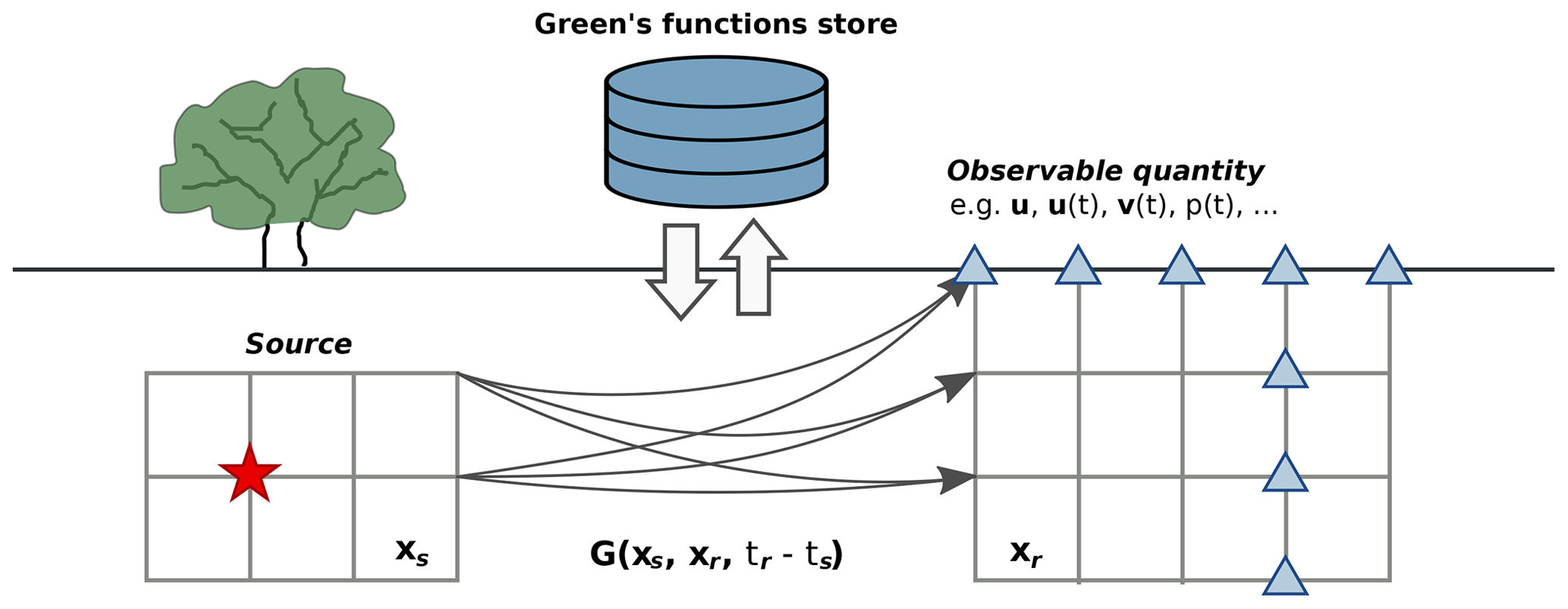
Figure 1Concept of the Green's function stores, the positions of the source xs, and the positions of receivers xr from source–receiver pairs of Green's functions that are computed on a predefined grid for a specified time window. These GFs are saved in a store and can be utilised through the Pyrocko-GF Python API.
The aim of our work is to provide a stand-alone open-source toolbox for the calculation and storage of GFs, suited for an easy integration into individual routines. To achieve this, we made our framework independent of the GF type and the GF calculation method that synthesises the physical quantities. The architecture of the GF stores is flexible to allow for the storage of extra attributes, e.g. travel time tables. We put special effort into finding a good balance between stability, numerical performance, and user-friendly implementation. While being part of the Pyrocko software library, our framework is easily linked to other seismological Python toolboxes, e.g. Pyrocko (Heimann et al., 2017) or ObsPy (Krischer et al., 2015).
Similarly to the seismological projects Instaseis and Syngine, we also openly share various existing GF stores at https://greens-mill.pyrocko.org (last access: 23 October 2019).
The paper is organised as follows: Sect. 2 describes the theoretical framework and GF definitions used in the proposed Pyrocko-GF infrastructure. Section 3 refers to the implementation design, and Sect. 4 gives examples of seismological applications.
2.1 Basic approach
For the following notations it generally applies that (1) vectors, tensors, and matrices in symbolic notations are shown as bold-faced symbols, (2) index notations are expressed with the Einstein summation rule, and (3) coordinates refer to either Cartesian coordinate systems with x–y–z or north-east-down (N-E-D) or to an axisymmetric polar coordinate system with radial–tangential–vertical (r–φ–z, with φ oriented clockwise and z oriented down). We denote a Green's function by , where xr and xs are receiver and source point positions, respectively. The time difference tr−ts is the difference between the receiver time tr and the time ts of the delta-pulse force excitation at the source. We assume vector forces at the source and vector fields as observed variables at the receiver position. The GF is represented by a 2nd-order tensor, as the three components of the observed vector can be excited by three forces acting in three different directions. Let u be the observed displacement vector field at the receiver located at the surface and f be the force vector density acting in the source volume V; the GF representation is then given by
The observed quantity is a superposition of all forces acting in the source volume, convolved with the individual timing of force excitation. In the second GF representation (Eq. 1) the convolution integral is replaced by the symbol ∗, omitting the time variable t. The convolution in Eq. (1) can be rewritten as a matrix equation in any coordinate system convenient for numerical implementation, with three-dimensional data vector u and source vector f, and a 3×3 matrix C of GF components as
While Eq. (1) is valid in general, a buried seismic source can also be represented by generalised force couples m, localised on a planar surface with an area A (rupture plane). The generalised force couples m form a symmetric, 2nd-order moment tensor density. In such a moment tensor representation, the GF tensor has 27 instead of 9 components. It relates to the 1st- and 2nd-order spatial derivatives of the single-force GF (denoted by a comma-separated last index) as (e.g. Aki and Richards, 2002)
with i,j, and in Cartesian coordinates. In , the superscript index i is the displacement direction, while the subscripts j and k indicate the force direction and force arm, respectively.
A matrix formulation of the index-notated Eq. (3) is obtained by mapping the symmetric moment tensor m into a source vector of length 6. Accordingly, the Green's tensor becomes a 3×6 matrix:
Due to the symmetry of the moment tensor, the GF matrix in general has only 18 independent components: , , and .
The given matrix formulation is convenient for an efficient numerical implementation in the GF store and it allows for a generalisation of mixed problems. For example, let u in Eq. (3) be a mixed-data vector b observed at the receiver, consisting of ground displacements u and rotational motions ω. Also, let the source vector s be represented by a mixed-type force system, wherein force couples and single forces act together within the source volume V. Then, the matrix representation of the mixed problem can be written as
Note that in Eq. (5) C contains GF components of different units. If the GF components C are known over the range of potential source and receiver positions as well as over the relevant time lags, the observables due to arbitrary source models can be synthesised using Eq. (5) by approximating the temporal and spatial integrals with sums (e.g. Dahm and Krüger, 2014).
2.2 Green's tensor and source models in layered elastic media
The number of independent GF components can be further reduced for media of cylindrical symmetry in a flat-Earth model or of spherical symmetry in a spherical-Earth model. For a GF tensor that is calculated for a station at zero azimuth we use the variable 0G. Considering geometric symmetries at zero azimuth (north direction), P-wave motion and vertically polarised S-wave (SV) motion can only be excited by the moment tensor components mxx, myy, mzz, mxz, and mzx. Similarly, horizontally polarised S-wave (SH) motion can only be excited by the moment tensor components mxy and myx. This reduces 0G to the form (Dahm, 1996; Heimann, 2011; Dahm and Krüger, 2014)
This reduces the number of independent GF components to 10 (e.g. Mueller, 1985). These GF components depend only on the source depth, the distance to the receiver, and the receiver depth.
A layered medium is invariant to rotation around z at the source element. We exploit this cylindrical symmetry to derive GFs in the r–φ–z direction at a station with a given azimuth through a tensor rotation with the azimuth angle φ:
Note that index i′ is in the r–φ–z coordinate system, while i is in the local x–y–z coordinate system at the source (equivalent to north-east-down). Thus, with Eq. (7), the convolution of m with G (Eq. 3) is derived component-wise as
with
The calculation of synthetic displacements is a linear combination of 10 GF components , here elementary seismograms, with the moment tensor components as weighting factors. These GF components are placed into a GF store. The GF components and are near-field terms and do not add to regional or teleseismic observations of dynamic displacements (Aki and Richards, 2002).
The GF representation from Eq. (8) can be re-ordered in the form of the matrix notation (Eq. 5)
where b is the observed data vector (here components of displacements), s is the source vector (here components of moment tensors), and C is the matrix form of the GF components. This form is suited for a mixed-type implementation (Eq. 5) and it also allows for a simple projection of {C∗s} a priori to components of the data vector. These projections can be useful, for example, to project to the ray system (L–Q–T), to inclined borehole sensors, or to transform the r–φ–z coordinate system to an N-E-D coordinate system of the sensor.
3.1 Green's function store architecture, schemes, and storage format
Green's function stores consist of a discrete, sparse, and truncated representation of the in Eq. (8). Time-dependent 1-D arrays (GF traces) are stored for a finite grid of source and receiver positions or of relative coordinates, resembling a finite spatial extent (Fig. 1). The GF traces are stored in a single binary file traces, which allows for efficient reading of the stored data. Lookup indices for accessing the GF traces are stored in the binary file index (for technical details, see Heimann et al., 2017, https://pyrocko.org/docs/current/formats/gf_store.html, last
access: 5 November 2019). Start and end times of the GF traces may be different for every node to allow for the compact storage of application-relevant portions of the waveforms (e.g. P or S phases, surface waves, etc.). A repeating end-point condition is assumed when extracting waveforms from the store. This way, a step function can be represented by just two samples at every node (e.g. for the modelling of static displacement changes). The strategy we follow to build synthetic data vectors for arbitrary source–receiver locations by using the discretised GF is described below in Sect. 3.2.
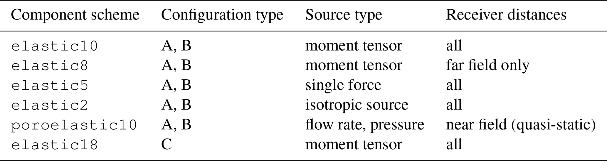
We categorise several store configuration types that are tailored to specific groups of source–medium–receiver configurations. The physics of the modelled process and the symmetry of the medium determine the number of GF components that are needed to represent the effects of a source at a receiver site (Table 1). For example, in a medium of cylindrical symmetry with a planar layered medium and at short distances, the simulation of a full moment tensor requires 10 GF components; a single force or isotropic source only needs 5 or 2 components, respectively. Also, for receivers located in the far field, the number of necessary components is reduced. The combination of these categories defines the structure of the store (Table 1). Such a flexible design also allows users to store the GFs of other transfer functions, e.g. to simulate the poro-elastic behaviour of a medium. This categorisation allows us to provide the efficient calculation, storage, and reading of GFs for problems of lower dimensions. Consequently, the generation of synthetic quantities, e.g. seismograms, is efficient.
Table 1Green's tensor component schemes and configuration types for GF stores. Configuration types A and B stand for rotation-symmetric media with (A) common-depth receivers or (B) variable-depth receivers. Configuration type (C) is used for three-dimensionally heterogeneous media with sources in a defined source volume and receivers at fixed positions.
The range and spacing of source locations, depths, and lateral source–receiver distances, along with the time span and the sampling rate of the GF traces and other metadata, are defined in a configuration file, config. The config file also contains the medium model definitions, i.e. seismic velocities, densities, and attenuation coefficients. The selection of a component scheme and configuration type defines the mapping used to transform physical source–receiver coordinates into the file lookup indices used in the index file.
The config is defined in the human-readable YAML Ain't Markup Language (YAML) structured YAML format. This eases the inspection of the metadata and the file can easily be edited with any text editor. The configuration file can be created and edited either manually or automatically by using the API. For details on the binary encoding and the YAML data structure, please see Heimann et al. (2017, Pyrocko GF store file format).
In addition to the mentioned files traces, index, and config, the store comprises two directories, extra and phases. They contain the individual GF-method-related configuration file(s) and, in the case of waveform problems, the travel time tables for user-specified arrivals. Providing travel time tables consistent with the GFs is useful in practical applications, e.g. to extract specific seismic phase arrivals.
Once created, the grid of traces in a GF store may be decimated in space and time. Such a downsampled version may be placed in an individual store or in the sub-directory decimated of the parent GF store. A downsampled store can be read faster and synthetic quantities are calculated faster. This can be useful, e.g. to simultaneously simulate high-frequency body waves and long-period surface waves by using the full resolution store and the downsampled store, respectively.
3.2 Green's function computational back end modules
The Green's functions depend on the Earth model and the problem geometry. As scientific applications differ, several specialised numerical methods have been developed to calculate GFs. For instance, reflectivity-type wavenumber integration methods (e.g. QSEIS; Wang, 1999) are commonly used to calculate high-frequency body waves and surface waves from teleseismic to local distances. Direct integration (e.g. GEMINI; Friederich and Dalkolmo, 1995) or hybrid methods (e.g. QSSP; Wang et al., 2017) are established for long-period global seismology on a spherical Earth. QSSP can also be used to simulate the coupling between the solid Earth, ocean, and atmosphere, including gravity waves and infrasound, or to calculate the elasto-gravitational effect from elastic wave propagation. The program AxiSEM (Nissen-Meyer et al., 2014), as employed by Instaseis (Van Driel et al., 2015), provides seismic wave fields for a 3-D axisymmetric Earth structure. Layered elasto-static and gravity problems in seismology and volcanology are often approached with methods adopted from Haskell-type integration (e.g. PSGRN/PSCMP; Wang et al., 2006). Poro-elastic quasistatic problems of fully coupled deformation and flow in layered media can be handled using orthonormal Haskell-type integration (e.g. POEL; Wang and Kümpel, 2003). These GF calculation methods assume horizontally layered medium models, apart from AxiSEM, which requires axisymmetric heterogeneity only.
Different GF computation methods are implemented with different model parameter conventions (e.g. for the different coordinate systems, source model descriptions, etc.). They are also written in different programming languages (e.g. Fortran or C). Therefore, we designed the structure of the GF store to be independent from the calculation method of the GFs. A standardised set-up and configuration is ensured by so-called back ends, written as Python modules. These back ends transfer the output of the respective GF computation method to the data format of the GF store. Such a concept enables the implementation of various existing or future GF calculation methods. The structured filling process of the store allows for the parallel computation of GFs to efficiently exploit the computer systems at hand.
At the time of publication we have implemented back ends for QSEIS, QSSP, PSGRN/PSCMP, and POEL to be installed individually and to be used with the Python toolbox Pyrocko (Fig. 2a and Heimann et al., 2017). In addition to these external code back ends, Pyrocko includes its own method AHFULLGREEN. This back end calculates GFs for an analytical, homogeneous full space (Aki and Richards, 2002) including near-, intermediate-, and far-field wave components. It can be applied to simulate acoustic emissions in mines or laboratory probes, or it can be useful for lecturing purposes. The chosen structure is not limited to GFs of force excitation. Also, GFs simulating other processes could be handled through GF stores, e.g. flow rate and pressure pulses. Only the implementation of a method-related back end is needed here.
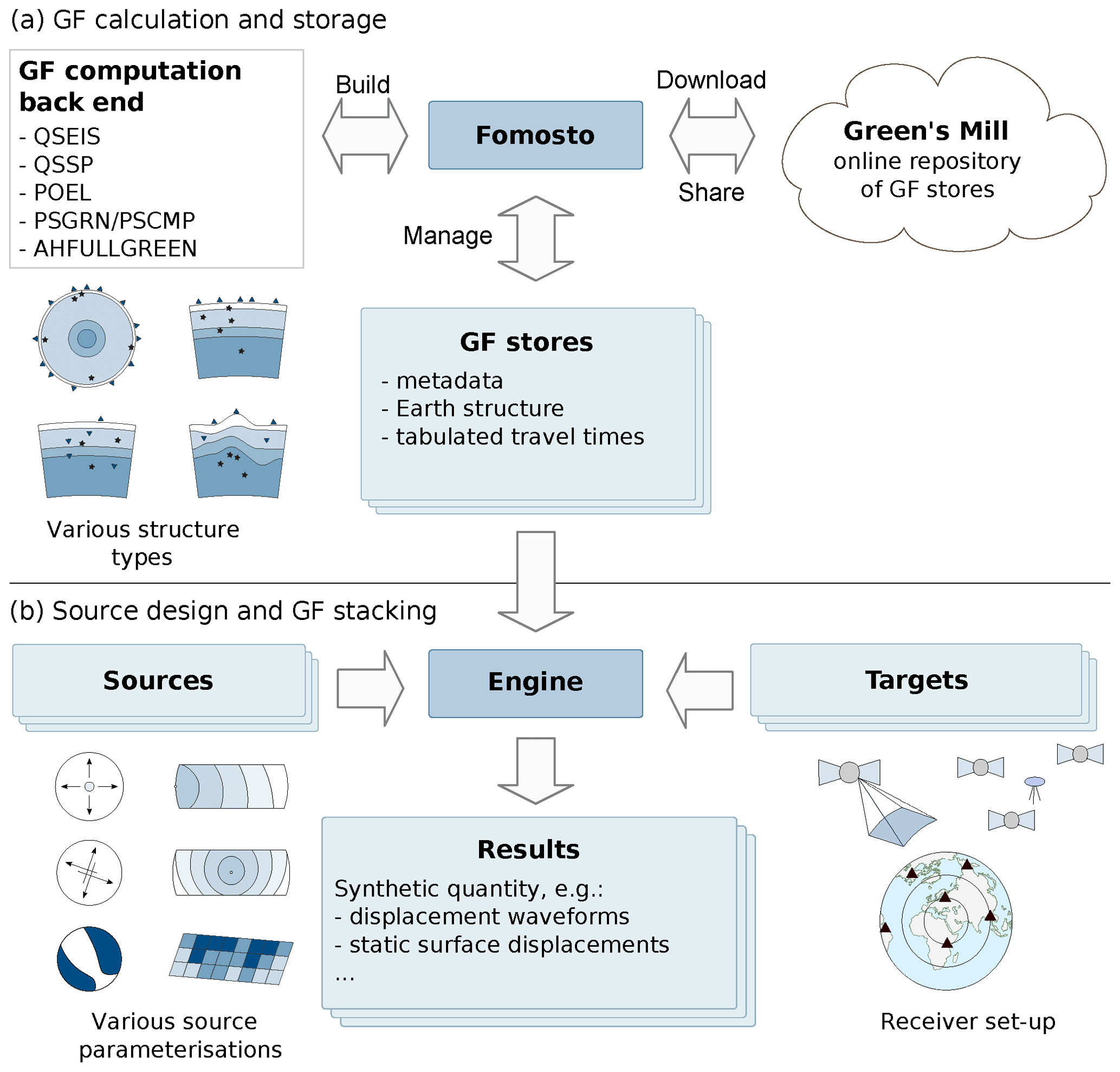
Figure 2The architecture of Pyrocko-GF and the object-oriented implementation scheme. (a) The fomosto program is a command-line interface (CLI) to create GFs using the back ends to inspect and manage GF stores. (b) The engine is the central object that accesses the computed Green's function stores and calculates the synthetic waveforms based on the specified source (e.g. moment tensor, double-couple source, or finite rectangular) and targets (e.g. virtual seismometers, GNSS stations, or InSAR line-of-sight displacements).
3.3 Source design
To simulate the physical quantity related to points of force excitations (sources), several GF traces from the pre-calculated store are combined. In the following, we illustrate the concept of source design based on a rectangular dislocation source that is finite in space and time, with uniform slip, a rupture nucleation point, and a rupture velocity.
The calculation of an observed quantity of interest (e.g. seismic waveforms) for a point source with delta-force excitation at a particular source–receiver constellation is given in Sect. 2. As described above, the specific combination of GF components is defined by the source type and the observed type of quantity (e.g. a full moment tensor or a single force, generating far-field waveforms or surface displacements; see Table 1).
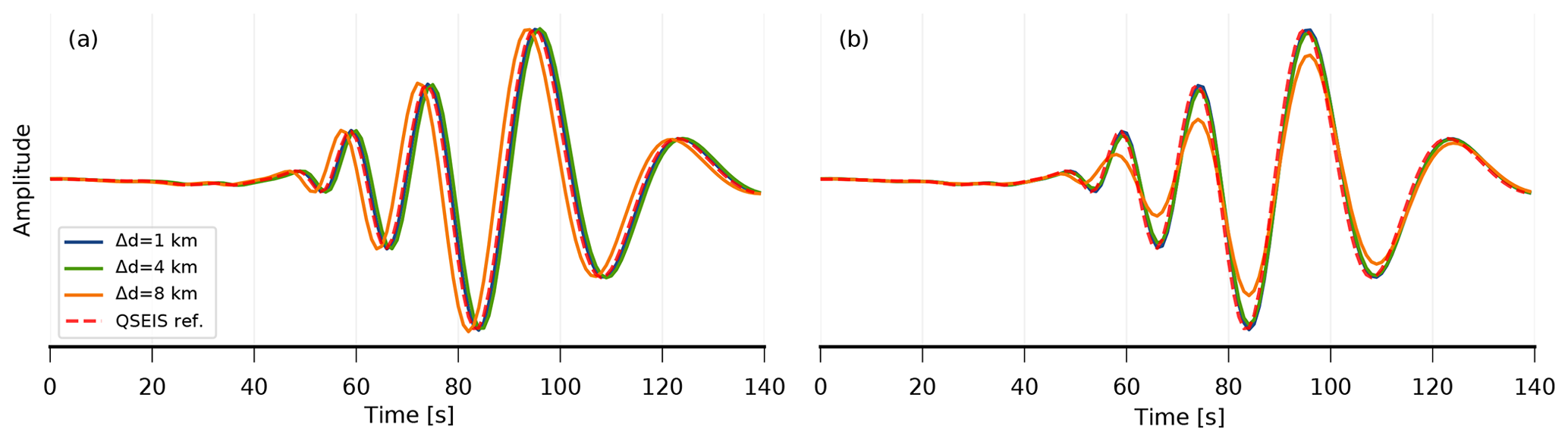
Figure 3Comparison of interpolation artefacts on synthetic waveforms with different GF grid spacings (a: nearest neighbour, b: multi-linear). Shown are vertical component displacements based on GF stores with 1, 4, and 8 km spatial grid spacing (blue, green, and orange, respectively) against a reference for the exact source–receiver distance (QSEIS; red). The sampling rate is 2 Hz and the signal contains information up to close to the Nyquist frequency (1 Hz). The waveforms are filtered with a pass band from 0.05 to 0.1 Hz after interpolation. The medium is layered with important discontinuities of upper crust, lower crust, and mantle at 20 and 35 km of depth. The slowest seismic velocity in the medium is 3.5 km s−1. The waveform is simulated for a 10 km deep moment tensor source at a distance of 553.3 km.
The observed quantity at the receiver is a linearly weighted combination of the spatially closest GF components. Often, this requires interpolation to match the requested source–receiver configuration. The interpolation of GF components requires an appropriate density of grid nodes to result in seismograms that are accurate in amplitude and phase (Fig. 3). Furthermore, simulated seismograms vary for different interpolation methods such as nearest-neighbour or multi-linear interpolation. For standard applications with multi-linear interpolation, we could require that the grid spacing dgrid should be less than a quarter of the minimum wavelength. It can be estimated using the minimum wave velocity vmin and the maximum signal frequency of the GF traces fmax with . For applications requiring higher accuracy, a smaller grid spacing must be used. For static displacements in the near field of finite sources discussed below, an appropriate grid spacing is smaller than half the minimum source–receiver distance. In general, smaller grid spacing leads to higher accuracy at the cost of forward modelling performance and larger GF stores. The interpolation of GF components in the spectral domain is superior but computationally more demanding (Gülünay, 2003).
To constrain the finite duration of moment release at a source point, we extend the delta-force excitation to force excitations in time, which is known as the source–time function (STF). Common STF types are triangular, half-sinusoidal, boxcar, or smooth ramp (Brüstle and Müller, 1983; Udias et al., 2014). All of these are defined through a source duration parameter and STF-specific parameters, e.g. the peak moment for a triangular STF. The temporal discretisation of finite-duration source models corresponds to the temporal sampling of the stored GF traces, ΔtGF.
The linear combination of several of these point sources allows us to construct spatially finite sources. For example, a rectangular source can be expressed with point sources that are aligned on a rectangular grid outlining the area of the finite source. The source area is defined by the length and width of the rectangular plane and its strike and dip. In combination with the rake angle and the amount of slip on the rupture plane, the mechanisms of the dislocation and the moment are defined. The nucleation point of the rupture across the fault is defined relative to the centre of the rectangular plane.
The spatial distance of point sources on the plane is controlled by the spatial discretisation of the stored GFs (ΔzGF and ΔxGF). The point-source spacing is also constrained by the temporal sampling intervals ΔtGF and the minimum possible rupture velocity vrupt,min. The distance between point sources, Δsrc, should either be smaller than half the minimum GF grid spacings or half the distance it takes the rupture to propagate in ΔtGF:
Accordingly, the integer number of equally spaced point sources NL,src along the length of a rectangular, planar source Lsrc is
The same relations apply for the number of sources across the rectangular plane NW,src of width Wsrc. Thus, the total number of point sources Nsrc that build the finite source is . In the case that the point sources contribute equally to the moment of the finite source, the point-source moment is the total moment divided by the number of point sources Nsrc. In general, the sum of all point-source moments is the total moment of the discretised source.
Finally, we define the rupture propagation across the rupture plane by the rupture velocity vrupt. The rupture starts at the nucleation point and from there propagates radially across the fault. The other point sources start rupturing with a time shift of tshift,i at the ith point source. This time shift depends on the distance di between the point source and the nucleation point as well as the mean rupture velocity between these two points:
With a similar strategy many more finite-source types can be realised using Pyrocko-GF (for details, see Sect. 3.5 and the online documentation at https://pyrocko.org/docs, last access: 23 October 2019).
Once the source model has been discretised into an ensemble of point sources in space and time, a discrete approximation of Eq. (1) can be used to calculate a synthetic seismogram or any other observable quantity at a receiver site. The sample u[i] at discrete time i can be computed from a sum of weighted and time-shifted GF contributions as
where w[j] represents weighting coefficients and k[j] represents delay times. The index j selects the stored GF trace and is a mapping of source position, receiver position, and the GF component index. If it is required to interpolate between the nodes of stored GFs, multiple such contributions from a neighbourhood in GF space are added. Similarly, time interpolation can be implemented by adding weighted and time-shifted GF contributions. The weights w[j] are computed considering (1) a rotation at the source (from the source coordinate system to the GF coordinate system), (2) a rotation at the receiver (from the GF coordinate system to the receiver component orientations), and (3) the involved interpolations. Our implementations of source design and the GF stacking approach in Pyrocko-GF take into account additional practical considerations to provide an efficient, flexible, and easy-to-use modelling engine.
3.4 Computation and quality checks of Green's function stores
With the user interface fomosto (FOrward MOdeling and Storage TOol) we provide a tool to create, manage, and inspect GF stores. Fomosto builds the GF stores and facilitates the calculation of the GFs through the back ends. Furthermore, fomosto features chopping of the GF traces to travel-time-relative time windows before their insertion into the GF store. This reduces the amount of stored data and removes synthetic seismogram parts prone to high contamination by numerical noise. Another store-managing feature of fomosto is the spatial and temporal decimation of the GF store (Sect. 3.1). Last but not least, fomosto-built GF stores can be accessed by the Pyrocko project for many forward modelling applications (see Sect. 3.5).

Figure 4Synthetic seismogram distance section generated by the report sub-command of fomosto (generated by command fomosto report single min_config wherein min_config is a configuration file). Vertical component seismograms are calculated for a given moment tensor source for a given frequency range and distance range provided in the GF store (0.25–0.5 Hz at 0–500 km of distance). Theoretical first arrivals (P body waves) and other travel time curves are plotted together with synthetic seismograms. Such a display is useful to identify numerical artefacts. Here, an acausal numerical phase running with a negative velocity into negative times at distances below 50 km can be found.
The quality control of the ensemble of GF traces is not trivial. GF stores can contain GFs for a large number of source and receiver positions such that a complete visual control by the scientist is impossible. In order to facilitate quality control, fomosto offers several options for visual inspection. In a report generated with its report sub-command, the GF traces are assembled in specified time windows in predefined frequency ranges together with predicted travel time arrivals (Fig. 4). The standard report produces plots of displacement and velocity traces, plots of maximum amplitudes, and plots of displacement spectra from the GF traces in the analysed store(s). These plots help identify spurious signals or numerical artefacts in synthetic seismograms. The reports can be customised through a dedicated configuration file. Fomosto can also be used to visualise the metadata of the GF store, e.g. the Earth model of seismic velocities or the associated travel time tables.
The computational effort to create a GF store depends on the complexity of the medium model, the temporal and spatial sampling, and the duration of the desired waveforms. For example, a global database based on the Preliminary Reference Earth Model (PREM), calculated with QSSP with 2 s sampling and 4 km spatial spacing in distance and source depth, requires an effort of about 19 h on a 100-core Intel Xeon E7-8890 high-performance computer and uses 52 GB of disc space. For comparison, regional GF stores at 2 Hz maximum frequency are built within hours on modern desktop computers.
To avoid redundant calculations, pre-calculated GF stores are provided for download on the Green's Mill web service under https://greens-mill.pyrocko.org (last access: 23 October 2019). As of today, GF stores for global and regional applications are provided for a set of different global Earth models and individual layered regional models adapting selected CRUST 2.0 velocity profiles1. GF stores developed during new applications and external projects can be uploaded to the GF store web page Green's Mill.
3.5 Forward modelling programming interface
The Pyrocko-GF framework implements the described methods to utilise the GF stores for the forward modelling of seismic waveforms and near-field displacements. The framework is focused on various forward modelling applications in seismology and geophysics. The object-oriented programming model provides Source objects defining the dislocation source(s), Target objects defining the modelling target (e.g. seismometer or global navigation satellite system (GNSS) station components), and the Engine object responsible for forward modelling (Fig. 2b).
The Source objects define the source properties, which may include the location, mechanism, and origin time. The Source object is responsible for the discretisation of point- and finite-extent sources into their moment tensor representations for weighting the store's GF traces (see Eq. 8).
The Target object defines the parameters of the synthesised quantities such as the location of receivers and the requested quantity type. In addition, seismic targets can provide derivatives of the synthetic displacements (i.e. velocity and acceleration).
Source and Target locations are specified as geographic coordinates with an optional Cartesian offset. This design allows the user to handle global, local, and mixed set-ups. These different set-ups are achieved, respectively, by either setting the Cartesian offset to zero, by setting the geographic coordinates to a common reference location, or by using a combination of both.
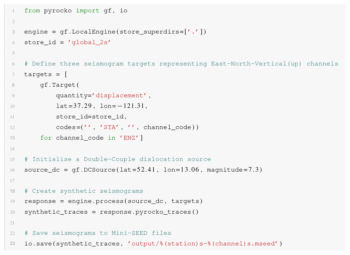
Listing 1Python script example for forward modelling a synthetic seismogram with the Pyrocko-GF framework. More complete examples are available at https://pyrocko.org/docs/current/library/examples/gf_forward.html (last access: 23 October 2019).
The Engine connects the Source and Target objects to the GF store.
Based on the configuration of Source and Target, the Engine extracts the required GF traces from the store and realises the stacking of delayed and weighted traces and their subsequent convolution with the Source's STF. Finally, the Engine returns the synthetics for the request defined by the Source and Target objects. An example illustrating the use of the Pyrocko-GF API is given in Listing 5.
In practice, the described stacking of GF traces is computationally demanding. Stored GF traces are time dependent and differ in length. Consequently, a stacking of these GF traces requires time shifting the GF traces and dynamic resizing of the output response. GF stores can become large, depending on resolution in time and space. To overcome limitations, we make use of the virtual memory mapping of files. Parallelised C extensions manage queries to the database and efficiently stack the GF traces according to the different component schemes (Sect. 3.1). An adaptive stacking scheme is available for waveforms and static models, which often have a very large number of source–receiver pairs. To ensure the correct complex interplay of functions software unit tests are carried out routinely.
The presented architecture in Pyrocko-GF enables the simple implementation of custom point and extended dislocation sources, as well as STFs. The framework's flexibility allows for the modelling of finite earthquake ruptures with variable STFs across the rupture plane (Vasyura-Bathke et al., 2019). The complete documentation of Pyrocko-GF's API is available online at https://pyrocko.org/docs/current/, featuring tutorials and examples of Python scripts and Jupyter notebooks.
4.1 Seismic and acoustic source inversion
Challenges in seismic source inversions include computational aspects, for instance the estimation of parameter uncertainties, and the aspect of a flexible definition of force representations for the specific rupture process under study.
Several groups of researchers use GF stores and the Pyrocko framework for source parameter estimation and centroid moment tensor inversion.
Examples include nuclear explosion source studies (Cesca et al., 2017; Gaebler et al., 2019), anthropogenically triggered events (Sen et al., 2013; Ma et al., 2018; Grigoli et al., 2018), sinkhole processes (Dahm et al., 2011), local and regional tectonic earthquakes (e.g. Dahm et al., 2018), magmatic-induced low-frequency earthquakes (Hensch et al., 2019), earthquakes related to caldera collapses (Gudmundsson et al., 2016; Cesca et al., 2019), landslides (Kulikova et al., 2016), and meteor explosions (Heimann et al., 2013).
These examples show that Pyrocko GF stores (in some cases its predecessors) have been applied to synthesise data from global, regional, and local seismic networks, with different frequency ranges and different wave modes (body waves, surface waves, W phases, etc.). Also, the range of studied source types is wide, including full moment tensors and double-couple, single-force, finite-extent earthquake, and point- or finite-extent volcanic sources.
A standard application is to estimate the parameters of a double-couple source from teleseismic data by using a GF store based on a global velocity model. We provide a commented step-by-step code example for the real-data optimisation of the 2009 L'Aquila earthquake (Italy) in the form of a Python Jupyter notebook at https://git.pyrocko.org/pyrocko/pyrocko-notebooks/src/master/Waveform_Inversion-Double-Couple.ipynb (last access: 23 October 2019).
A more exotic example is the source inversion of the Chelyabinsk meteor terminal explosion (Heimann et al., 2013). It demonstrates the flexibility towards specialised source types and GF stores involving the atmospheric layers. The Chelyabinsk meteor explosion occurred on 15 February 2013 near the town of Chelyabinsk, Russia, at an altitude of about 23 km. Through seismo-acoustic coupling, its shock wave generated Rayleigh waves that were observed at epicentral distances of up to 4000 km. We analysed these recordings with a modelling and inversion approach. Synthetic GFs for atmospheric, surface, and underground sources were calculated using the QSSP program (Wang et al., 2017), which can handle the coupling of the solid Earth and atmosphere. The inversion for source location and strength, including error analysis, was performed using Kiwi Tools (Heimann, 2011), a software for earthquake source inversion. The GF store approach allowed us to cleanly separate the inversion from the GF generation task with only minimal modifications applied to the two distinct code bases. The GF store used for the Chelyabinsk meteor explosion source inversion is available at https://greens-mill.pyrocko.org/42487ae804b0cfb219d7486ee1c10ee412fe12a3 (last access: 23 October 2019).
The separation of GF handling, source modelling, and inversion–optimisation encourages designing modular software architectures with well-defined interfaces. At the time of writing, two feature-rich, open-source earthquake analysis software packages rely on Pyrocko-GF for modelling and GF handling: the Bayesian Earthquake Analysis Tool (BEAT; Vasyura-Bathke et al., 2019), which implements Bayesian inference for source characterisation, and the probabilistic earthquake source inversion framework Grond (Heimann et al., 2018), which implements a Bayesian bootstrap technique.
4.2 Inverting near-field surface displacements during magma chamber evacuation
In geophysics, static displacement in the near field is often modelled assuming a homogeneous half-space, using analytical solutions (e.g. Mogi, 1958 or Okada, 1985). Many methods for modelling more realistic dislocation sources and media are available but at higher computational cost. A GF store approach can compensate for this obstacle and provide convenient access to a more complex modelling environment. Our fomosto tool facilitates the computation of static GF stores for layered media with its PSGRN/PSCMP (Wang et al., 2006) back end. To illustrate the use of Pyrocko-GF for static deformation modelling, let us examine a case study on the volcano–tectonic crisis in the Comoro Islands, which started in 2018 offshore of the island of Mayotte (Cesca et al., 2019).
On Mayotte four GNSS stations showed large horizontal displacements and subsidence of up to 20 cm over a period of more than 8 months; the distinct horizontal displacements point towards a deflation source situated offshore. We used the few near-field GNSS data to complement the seismic analysis in constraining the location and character of the deflation source. From the seismic analysis an upward migration of the seismicity from ∼20 km to shallower crustal levels was inferred (Cesca et al., 2019).
We tested different point dislocation sources and velocity–elasticity models against the observed GNSS data and evaluated the different models in a Bayesian inversion, provided by the Grond framework (Heimann et al., 2018). We found that an isotropic source model in a homogeneous half-space cannot adequately represent the observations. However, the observations are compatible with a constrained moment-tensor-based point-source model, representative for a vertically elongated, deflating ellipsoid, similar to the point compound dislocation model (Nikkhoo et al., 2016) or an ellipsoidal cavity (Davis, 1986; Segall, 2010, chap. 7). Such a tailored dislocation source and more realistic elasticity model derived from the AK135 model2 (Kennett et al., 1995) provide a more physical representation of the phenomenon and thus a better interpretation of the underlying geological processes.
In this case study, Pyrocko-GF provided a fast and efficient modelling framework, into which a newly designed source model could be plugged without requiring additional implementation work on the forward modelling itself. Seismic waveforms and static displacement are analysed in a homogeneous environment in terms of the Earth models and software toolset used.
4.3 Ground motion and shake map simulation
GF stores can be used to explore attenuation functions of ground motions and their uncertainties that are related to the variability of the source and the structural parameters of the medium. Such explorations can be applied in scenario simulations to support risk assessment procedures. Furthermore, it is possible to generate near-real-time ground motion forecasts after an earthquake. The Pyrocko-GF framework is sufficiently fast to allow for such near-real-time waveform simulations. The advantages of synthetic GF-based approaches to empirical relations of peak ground motion (Dahm et al., 2018) and magnitudes (Dahm et al., 2019) are (1) that regional Earth structure models can be taken into account and (2) that earthquake sources can be simulated in regions where natural earthquakes have not been recorded. The latter situation also arises in most cases of induced seismicity, for which hazard and risk assessment is of particular importance. A challenge in induced and micro-earthquake ground motion simulations is, however, to realistically simulate synthetic seismograms at sufficiently high frequencies.
Dahm et al. (2018) used a synthetic GF approach to validate peak velocity attenuation relations in central Germany, where damaging earthquakes struck in historical times but not during the instrumental period. Two similar GF stores were created to calculate peak ground velocity for two deep crustal earthquakes. One store contained GFs for a medium with a hard rock surface layer, while the other store had a soft sedimentary surface layer (find the corresponding GF stores crust2_m5_hard_top_16Hz and crust2_m5_16Hz at https://greens-mill.pyrocko.org (last access: 23 October 2019). GFs are pre-calculated for distances between 0 and 300 km and for source depths ranging between 0 and 35 km at intervals of 1 km with a sampling rate of 16 Hz. Peak ground velocities were extracted for 6 Hz low-pass-filtered seismograms (PGV6 Hz). The PGV6 Hz attenuation reproduced the observed averages and their variability well for the two deep crustal earthquakes, while empirical attenuation relations derived for other regions over- or under-predicted the observations. In Fig. 6 we show, as an example, PGV6 Hz shake map simulations for a magnitude MW 6.3 earthquake scenario near the cities of Leipzig and Halle, Germany3.
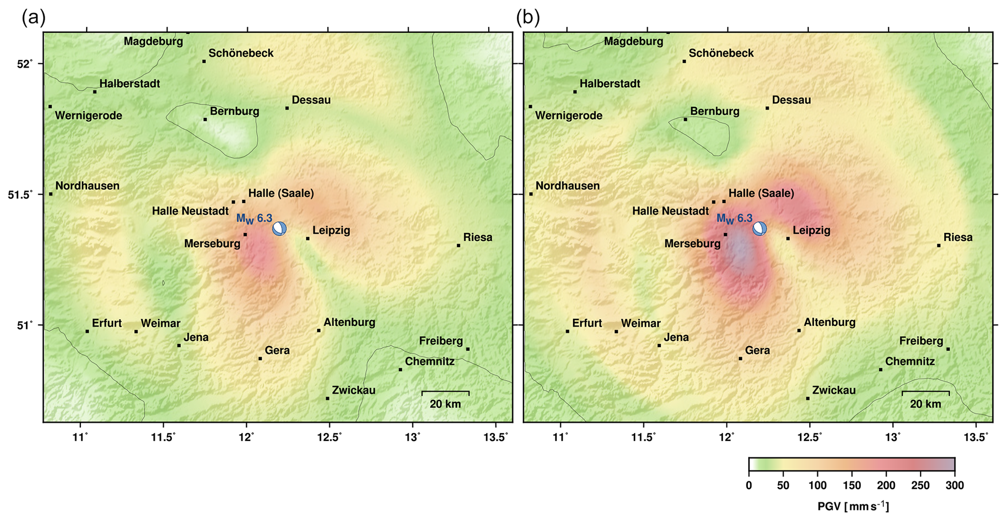
Figure 5Shake map scenario of a MW 6.3 characteristic lower-crust earthquake at 25 km of depth between Halle and Leipzig, Germany. (a) Predicted PGV6 Hz assuming a hard rock upper-layer model. (b) Predicted PGV6 Hz assuming a 500 m thick soft layer beneath the surface with P- and S-wave velocities of 2.5 and 1.2 km s−1, respectively. The contour line shows the 20 mm s−1 threshold (see Dahm et al., 2018, for further explanation).

Figure 6Illustration of waveform sensitivities caused by crustal velocity variations. (a) Colour-coded crustal P-wave velocity profiles as a function of depth. Darker colours correspond to lower crustal thickness. (b) Synthetic, low-pass-filtered seismograms of a double-couple point source corresponding to the P-wave velocity structure in (a) at 278 km of distance.
Peak ground motions of displacements or velocities are used to estimate earthquake magnitudes. Usually, empirical attenuation relations are used to normalise measured peak values and to estimate station magnitudes. The empirical relations are often poorly calibrated for the region under study and only valid for a narrow range of instruments, source depths, and strengths. GF stores can overcome some of the limitations of empirical attenuation curves in magnitude scales and can be used to estimate moment magnitudes from peak ground motions. Examples are provided in Dahm et al. (2019) for local magnitude estimations. Figure 7 gives an example of how the effect of different crustal models on full waveforms can be simulated on the fly4. This can be used, for instance, to explore the station variability of global surface wave magnitude scales.
4.4 Array and network design optimisation by full waveform simulation
The simulation of full waveforms for the directed Monte Carlo optimisation of seismic networks is computationally demanding and not standard in seismology. López-Comino et al. (2017) used synthetic GF stores for the simulation of full waveforms to predict the network performance and spatial and temporal variation of the magnitude of completeness before the deployment of stations. Synthetic velocity seismograms were generated and modified by real recorded noise based on a randomised catalogue of synthetic earthquake sources for a given source volume in the area under investigation. The seismograms were then used in a full waveform event detector to evaluate the expected magnitude of completeness.
For the design of a small-aperture array for the study of local micro-earthquakes, a synthetic GF store has been used by Karam Zadeh Toularoud et al. (2019). For a given distribution of synthetic hypocentres and source mechanisms that simulate an earthquake swarm, the authors randomly generated array locations and station configurations for which synthetic seismic waveforms were computed. For these synthetic set-ups the expected beam power and the slowness calculation error was optimised, which allowed the authors to judge a preferred array installation configuration. The array set-up was fixed to use seven stations with three components; 4000 different station configurations have been tested with 100 different sources each. Hence, a total number of 8.4 million traces had to be generated for the analysis. A desktop computer was sufficient for the computational task. Karam Zadeh Toularoud et al. (2019) used the GF store https://greens-mill.pyrocko.org/vogtland_malek2004_sed_HR-95ef03 (last access: 25 October 2019).
Pyrocko-GF is a Python module that provides functionality to calculate Green's functions (GFs) and to organise these in a store. In Pyrocko-GF, back ends utilise different numerical calculation methods for GFs, making the stores independent of the actual type of GFs. The command-line interface tool fomosto within the Pyrocko-GF framework manages the generation of GFs through the computational back ends, which so far exist for layered media. Fomosto also facilitates the comparison, visualisation, and quality check of stored GFs. The software is open source and encourages the contribution of use-specific extensions and adding interfaces to other computational back ends.
Our implementations support the computation of GFs useful for earthquake-related problems, which include GFs for broadband global, regional, and local seismograms, optionally with near-field terms, as well as static surface displacements as measured by GNSS sensors and/or through InSAR. Furthermore, Pyrocko-GF stores are prepared to store infrasound, oceanic infragravity, poro-elastic, and elasto-gravitational GFs. On the GF online platform Green's Mill (https://greens-mill.pyrocko.org, last access: 25 October 2019) we provide GF stores for download that are useful for many standard earthquake-related applications using global velocity models.
The Pyrocko-GF framework allows users to efficiently access GF stores to synthesise source-specific responses inside the medium for comparison with different observations. Sources and source–time functions can easily be customised without limitations on the source complexity. We discussed seismological applications using Pyrocko-GF stores to simulate seismic waveforms, static surface displacements and peak ground motion caused by earthquakes, volcanic activity, and exploding meteoroids. The range of applications is not limited to generalised force couples or single forces. With new back ends, flow rate, pressure pulse, or any other type of excitation and observable, which are representable using the GF approach, could also be included in a Pyrocko-GF store.
The presented software is available as open source under the GNU General Public License v3 and can be downloaded from https://git.pyrocko.org/pyrocko/pyrocko/ (last access: 25 October 2019). The documentation and examples are available at https://pyrocko.org (last access: 25 October 2019). Pre-computed Green's function stores can be browsed and downloaded at https://greens-mill.pyrocko.org/ (last access: 25 October 2019).
SH and TD are the scientific Pyrocko project leaders, supported by HS and HVB as scientific project partners. SH leads the software implementation to which HVB, MI, and MK have contributed significantly and in many ways, e.g. by writing parts of the codes. All authors contributed to the software design, the code testing, and the paper writing.
The authors declare that they have no conflict of interest.
Henriette Sudhaus, Andreas Steinberg, and Marius Paul Isken acknowledge funding by the German Research Foundation (DFG) through an Emmy-Noether Young Researcher Grant (276464525). Hannes Vasyura-Bathke was financially supported by the King Abdullah University of Science and Technology (KAUST) BAS/1/1353-01-01 as well as by Geo.X, the Research Network for Geosciences in Berlin and Potsdam (project number: SO_087_GeoX). Torsten Dahm and Sebastian Heimann acknowledge co-funding by SERA (EU grant 730900). Timothy Willey helped to implement fomosto report plots. We thank the University of Nevada, Reno, for processing and providing GNSS deformation data for Mayotte (Blewitt et al., 2018).
This research has been supported by the German Research Foundation (grant no. 276464525), the King Abdullah University of Science and Technology (grant no. BAS/1/1353-01-01), the EU SERA (grant no. 730900), and the Geo.X Research Network for Geosciences in Berlin and Potsdam (grant no. SO_087_GeoX).
The article processing charges for this open-access
publication were covered by a Research
Centre of the Helmholtz Association.
This paper was edited by Caroline Beghein and reviewed by Tim Greenfield and one anonymous referee.
Aki, K. and Richards, P. G.: Quantitative Seismology, University Science Books, 2nd Edn., available at: http://www.worldcat.org/isbn/0935702962 (last access: 25 October 2019), 2002. a, b, c
Blewitt, G., Hammond, W., and Kreemer, C.: Harnessing the GPS data explosion for interdisciplinary science, EOS, 99, https://doi.org/10.1029/2018EO104623, 2018. a
Brüstle, W. and Müller, G.: Moment and duration of shallow earthquakes from Love-wave modelling for regional distances, Phys. Earth Planet. In., 32, 312–324, https://doi.org/10.1016/0031-9201(83)90031-6, 1983. a
Cannell, D. M. and Lord, N. J.: George Green, Mathematician and Physicist 1793–1841, Math. Gaz., 77, 26–51, 1993. a
Cesca, S., Heimann, S., Kriegerowski, M., Saul, J., and Dahm, T.: Moment Tensor Inversion for Nuclear Explosions: What Can We Learn from the 6 January and 9 September 2016 Nuclear Tests, North Korea?, Seismol. Res. Lett., 88, 300–310, https://doi.org/10.1785/0220160139, 2017. a
Cesca, S., Letort, J., Razafindrakoto, H. N. T., Heimann, S., Rivalta, E., Isken, M. P., Nikkhoo, M., Passarelli L., Petersen, G. M., Cotton, F., and Dahm, T.: Drainage of a deep magma reservoir near Mayotte inferred from seismicity and deformation, submitted, 2019. a, b, c
Dahm, T.: Relative moment tensor inversion based on ray-theory: Theory and synthetic tests, Geophys, J. Int., 124, 245–257, 1996. a
Dahm, T. and Krüger: Moment tensor inversion and moment tensor interpretation, in: New Manual of Seismological Observatory Practice (NMSOP-2), edited by: Bormann, P. E., https://doi.org/10.2312/GFZ.NMSOP-2_IS_3.9, IASPEI, GFZ German Research Centre for Geosciences, Potsdam, 2014. a, b, c, d
Dahm, T., Heimann, S., and Bialowons, W.: A seismological study of shallow weak earthquakes in the urban area of Hamburg city, Germany, and its possible relation to salt dissolution, Nat. Hazards, 58, 1111–1134, https://doi.org/10.1007/s11069-011-9716-9, 2011. a
Dahm, T., Heimann, S., Funke, S., Wendt, S., Rappsilber, I., Bindi, D., Plenefisch, T., and Cotton, F.: Seismicity in the block mountains between Halle and Leipzig, Central Germany: centroid moment tensors, ground motion simulation and felt intensities of two M ≈ 3 earthquakes in 2015 and 2017, J. Seismol., 22, 985–1003, https://doi.org/10.1007/s10950-018-9746-9, 2018. a, b, c, d
Dahm, T., Cesca, S., Heimann, S., Maghsoudi, S., and Kühn, D.: A Greenfunction magnitude approach to overcome limitations of traditional magnitude scales, AGU 2017: 11–15 December 2017, New Orleans, Louisiana, 2019. a, b
Davis, P. M.: Surface deformation due to inflation of an arbitrarily oriented triaxial ellipsoidal cavity in an elastic half-space, with reference to Kilauea volcano, Hawaii, J. Geophys. Res.-Sol. Ea., 91, 7429–7438, https://doi.org/10.1029/JB091iB07p07429, 1986. a
Friederich, W. and Dalkolmo, J.: Complete synthetic seismograms for a spherically symmetric earth by a numerical computation of the Green's function in the frequency domain, Geophys. J. Int., 122, 537–550, 1995. a
Gaebler, P., Ceranna, L., Nooshiri, N., Barth, A., Cesca, S., Frei, M., Grünberg, I., Hartmann, G., Koch, K., Pilger, C., Ross, J. O., and Dahm, T.: A multi-technology analysis of the 2017 North Korean nuclear test, Solid Earth, 10, 59–78, https://doi.org/10.5194/se-10-59-2019, 2019. a
Grigoli, F., Cesca, S., Rinaldi, A. P., Manconi, A., Clinton, J. F., Westaway, R., Cauzzi, C., Dahm, T., and Wiemer, S.: The November 2017 Mw 5.5 Pohang earthquake: A possible case of induced seismicity in South Korea, Science, 5, 1003–1006, 2018. a
Gudmundsson, M. T., Jónsdóttir, K., Hooper, A., Holohan, E. P., Halldórsson, S. A., Ófeigsson, B. G., Cesca, S., Vogfjörd, K. S., Sigmundsson, F., Högnadóttir, T., Einarsson, P., Sigmarsson, O., Jarosch, A. H., Jónasson, K., Magnússon, E., Hreinsdóttir, S., Bagnardi, M., Parks, M. M., Hjörleifsdóttir, V., Pálsson, F., Walter, T. R., Schöpfer, M. P. J., Heimann, S., Reynolds, H. I., Dumont, S., Bali, E., Gudfinnsson, G. H., Dahm, T., Roberts, M. J., Hensch, M., Belart, J. M. C., Spaans, K., Jakobsson, S., Gudmundsson, G. B., Fridriksdóttir, H. M., Drouin, V., Dürig, T., Aðalgeirsdóttir, G., Riishuus, M. S., Pedersen, G. B. M., van Boeckel, T., Oddsson, B., Pfeffer, M. A., Barsotti, S., Bergsson, B., Donovan, A., Burton, M. R., and Aiuppa, A.: Gradual caldera collapse at Bárdarbunga volcano, Iceland, regulated by lateral magma outflow, Science, 353, 1–24, https://doi.org/10.1126/science.aaf8988, 2016. a
Gülünay, N.: Seismic trace interpolation in the Fourier transform domain, Geophysics, 68, 355–369, https://doi.org/10.1190/1.1543221, 2003. a
Heimann, S.: A Robust Method To Estimate Kinematic Earthquake Source Parameters, PhD thesis, University of Hamburg, Hamburg, 2011. a, b
Heimann, S., Gonzalez, A., Wang, R., Cesca, S., and Dahm, T.: Seismic characterization of the Chelyabinsk meteor's terminal explosion, Seismol. Res. Lett., 84, 1021–1025, 10.1785/0220130 042., 2013. a, b
Heimann, S., Kriegerowski, M., Isken, M., Cesca, S., Daout, S., Grigoli, F., Juretzek, C., Megies, T., Nooshiri, N., Steinberg, A., Sudhaus, H., Vasyura-Bathke, H., Willey, T., and Dahm, T.: Pyrocko – An open-source seismology toolbox and library, GFZ Data Services, V. 0.3, https://doi.org/10.5880/GFZ.2.1.2017.001, 2017. a, b, c, d
Heimann, S., Isken, M., Kühn, D., Sudhaus, H., Steinberg, A., Vasyura-Bathke, H., Daout, S., Cesca, S., and Dahm, T.: Grond – A probabilistic earthquake source inversion framework, GFZ Data Services, https://doi.org/10.5880/GFZ.2.1.2018.003, 2018. a, b
Hensch, M., Dahm, T., Ritter, J., Heimann, S., Schmidt, B., Stange, S., and Lehmann, K.: Deep low-frequency earthquakes reveal ongoing magmatic recharge beneath Laacher See Volcano (Eifel, Germany), Geophys. J. Int., 216, 2025–2036, https://doi.org/10.1093/gji/ggy532, 2019. a
IRIS DMC: Data Services Products: Syngine, IRIS DMC, https://doi.org/10.17611/dp/syngine.1, 2015. a
Karam Zadeh Toularoud, N., Heimann, S., Dahm, T., and Krüger, F.: Application based seismological array design by seismicity scenario modelling, Geophys. J. Int., 216, 1711–1727, https://doi.org/10.1093/gji/ggy523, 2019. a, b
Kennett, B. L., Engdahl, E., and Buland, R.: Constraints on seismic velocities in the Earth from traveltimes, Geophys. J. Int., 122, 108–124, 1995. a
Krischer, L., Megies, T., Barsch, R., Beyreuther, M., Lecocq, T., Caudron, C., and Wassermann, J.: ObsPy: a bridge for seismology into the scientific Python ecosystem, Computational Science & Discovery, 8, 17, https://doi.org/10.1088/1749-4699/8/1/014003, 2015. a
Krischer, L., Hutko, A. R., van Driel, M., Stähler, S., Bahavar, M., Trabant, C., and Nissen‐Meyer, T.: On‐Demand Custom Broadband Synthetic Seismograms, Seismol. Res. Lett., 88, 1127–1140, https://doi.org/10.1785/0220160210, 2017. a
Kulikova, G., Schurr, B., Krüger, F., Brzoska, E., and Heimann, S.: Source parameters of the Sarez-Pamir earthquake of 1911 February 18, Geophys. J. Int., 205, 1086–1098, 2016. a
López-Comino, J., Cesca, S., Kriegerowski, M., Heimann, S., Dahm, T., Mirek, J., and Lasocki, S.: Monitoring performance using synthetic data for induced microseismicity by hydrofracking at the Wysin site (Poland), Geophys. J. Int., 210, 42–55, https://doi.org/10.1093/gji/ggx148, 2017. a
Ma, J., Dineva, S., Cesca, S., and Heimann, S.: Moment tensor inversion with three-dimensional sensor configuration of mining induced seismicity (Kiruna mine, Sweden), Geophys. J. Int., 213, 2147–2160, https://doi.org/10.1093/gji/ggy115, 2018. a
Mogi, K.: Relations between the eruptions of various volcanoes and the deformations of the ground surfaces around them, B. Earthq. Res. I. Tokyo, 36, 99–134, 1958. a
Mueller, C. S.: Source pulse enhancement by deconvolution of an empirical Green's function, Geophys. Res. Lett., 12, 33–36, https://doi.org/10.1029/GL012i001p00033, 1985. a
Nikkhoo, M., Walter, T. R., Lundgren, P. R., and Prats-Iraola, P.: Compound dislocation models (CDMs) for volcano deformation analyses, Geophys. J. Int., 208, 877–894, https://doi.org/10.1093/gji/ggw427, 2016. a
Nissen-Meyer, T., van Driel, M., Stähler, S. C., Hosseini, K., Hempel, S., Auer, L., Colombi, A., and Fournier, A.: AxiSEM: broadband 3-D seismic wavefields in axisymmetric media, Solid Earth, 5, 425–445, https://doi.org/10.5194/se-5-425-2014, 2014. a
Okada, Y.: Surface deformation due to shear and tensile faults in a half-space, B. Seismol. Soc. Am., 75, 1135–1154, 1985. a
Segall, P.: Earthquake and volcano deformation, Princeton University Press, 2010. a
Sen, A., Cesca, S., Bishoff, M., Meier, T., and Dahm, T.: Automated full moment tensor inversion of coal mining induced seismicity, Geophys. J. Int., 195, 1267–1281, https://doi.org/10.1093/gji/ggt300, 2013. a
Tolstoy, I.: Wave propagation, McGraw-Hill, New York, 1973. a
Udias, A., Madariaga, R., and Buforn, E.: Source mechanisms of earthquakes: theory and practice, Cambridge University Press, Cambridge, UK, 2014. a
van Driel, M., Krischer, L., Stähler, S. C., Hosseini, K., and Nissen-Meyer, T.: Instaseis: instant global seismograms based on a broadband waveform database, Solid Earth, 6, 701–717, https://doi.org/10.5194/se-6-701-2015, 2015. a, b
Vasyura-Bathke, H., Dettmer, J., Steinberg, A., Heimann, S., Isken, M., Zielke, O., Mai, P. M., Sudhaus, H., and Jónsson, S.: BEAT – Bayesian Earthquake Analysis Tool. V. 1.0, GFZ Data Services, https://doi.org/10.5880/fidgeo.2019.024, 2019. a, b
Wang, R.: A simple orthonormalization method for stable and efficient computation of Green's functions, B. Seismol. Soc. Am., 89, 733–741, 1999. a
Wang, R. and Kümpel, H.-J.: Poroelasticity: Efficient modeling of strongly coupled, slow deformation processes in a multilayered half‐space, Geophysics, 68, 705–717, 2003. a
Wang, R., Lorenzo-Martín, F., and Roth, F.: PSGRN/PSCMP – a new code for calculating co- and post-seismic deformation, geoid and gravity changes based on the viscoelastic-gravitational dislocation theory, Comput. Geosci., 32, 527–541, https://doi.org/10.1016/j.cageo.2005.08.006, 2006. a, b
Wang, R., Heimann, S., Zhang, Y., Wang, H., and Dahm, T.: Complete synthetic seismograms based on a spherical self-gravitating Earth model with an atmosphere-ocean-mantle-core structure, Geophys, J. Int., 210, 1739–1764, https://doi.org/10.1093/gji/ggx259, 2017. a, b
http://igppweb.ucsd.edu/~gabi/rem.html (last access: 25 October 2019).
GF store: https://greens-mill.pyrocko.org/ak135_static-b18151 (last access: 23 October 2019).
See shake map code example at https://pyrocko.org/docs/current/library/examples/gf_forward.html (last access: 23 October 2019).
See Rayleigh wave waveform variability code example at https://pyrocko.org/docs/current/library/examples/gf_forward.html (last access: 23 October 2019).