The imprints of contemporary mass redistribution on local sea level and vertical land motion observations

Observations from permanent Global Navigation Satellite System (GNSS) stations are commonly used to correct tide-gauge observations for vertical land motion (VLM). We combine GRACE (Gravity Recovery and Climate Experiment) observations and an ensemble of glacial isostatic adjustment (GIA) predictions to assess and evaluate the impact of solid-Earth deformation (SED) due to contemporary mass redistribution and GIA on VLM trends derived from GNSS stations. This mass redistribution causes relative sea-level (RSL) and SED patterns that not only vary in space but also exhibit large interannual variability signals. We find that for many stations, including stations in coastal locations, this deformation causes VLM trends on the order of 1 mm yr⁻¹ or higher. In multiple regions, including the Amazon Basin and large parts of Australia, the SED trend flips sign between the first half and second half of the 15-year GRACE record. GNSS records often only span a few years, and due to these interannual variations SED causes substantial biases when the linear trends in these short records are extrapolated back in time.

We propose a new method to avoid this potential bias in the VLM-corrected tide-gauge record: instead of correcting tide-gauge records for the observed VLM trend, we first remove the effects from GIA and contemporary mass redistributions from the VLM observations before computing the VLM trend. This procedure reduces the extrapolation bias induced by SED, and it also avoids the bias due to sea-floor deformation: SED includes net sea-floor deformation, which is ignored in global-mean sea-level reconstructions based on VLM-corrected tide-gauge data. We apply this method to 8166 GNSS stations. With this separation, we are able to explain a large fraction of the discrepancy between observed sea-level trends at multiple long tide-gauge records and the global-mean sea-level trend from recent reconstructions.

1 Introduction

Recent global and local studies have shown that local vertical land motion (VLM) explains a significant part of spatial variations in tide-gauge trends, which, if ignored, biases estimates of global and local sea-level changes (e.g., King et al., 2012; Wöppelmann et al., 2014; Hamlington et al., 2016). Global and local sea-level studies therefore often use Global Navigation Satellite System (GNSS) records to correct tide-gauge records for VLM (Santamaría-Gómez et al., 2012; Dangendorf et al., 2017; Frederikse et al., 2018). Despite yielding significant improvements, such a correction does introduce two problems:

1. The resulting sea-level observations are essentially geocentric sea-level (GSL) observations. Global and local reconstructions based on these corrected records reconstruct GSL changes. Since not only the sea surface but also the sea floor can move vertically, global-mean GSL, which is blind to movements of the sea floor, deviates from the total change in ocean volume. As a result, global-mean GSL reconstructions could be biased with respect to global-mean sea-level (GMSL) changes, which are defined as the total change in ocean volume divided by the ocean area (Frederikse et al., 2017; Lickley et al., 2018; Gregory et al., 2019).

2. It is commonly assumed that the linear VLM trend, derived over the length of the GNSS record, which is typically a few years, is representative of the full time span of the associated tide gauge, which often covers multiple decades. This assumption generally holds for VLM caused by glacial isostatic adjustment (GIA) outside low-viscosity regions (e.g., Whitehouse, 2018), sediment isostatic adjustment, and compaction (Ferrier et al., 2017). However, for processes such as subsidence due to local groundwater depletion (Kolker et al., 2011; Minderhoud et al., 2017) and coseismic and postseismic activity (Segall and Davis, 1997), this assumption does not hold. Therefore, the extrapolation of the derived linear VLM trend over the short GNSS time span over the long tide-gauge records can introduce a bias (Featherstone et al., 2015).

Contemporary mass redistribution contributes to both problems: when mass is moved over the Earth surface, the Earth deforms elastically as a response to these changes in the load (Farrell, 1972). This solid-Earth deformation (SED) translates into local VLM that is registered by GNSS stations. Mass loss from glaciers and ice sheets and changes in terrestrial water storage (TWS) have resulted in an increase in ocean mass and a rise in global-mean sea level over the past decades (WCRP Global Sea Level Budget Group, 2018), but they have also caused substantial local SED patterns (Riva et al., 2017; Spada, 2017). This process explains a nonnegligible part of VLM signals observed by permanent GNSS stations (Santamaría-Gómez and Mémin, 2015; Pfeffer et al., 2017; Schumacher et al., 2018). Due to the accelerating pace of ice mass loss (Bamber et al., 2018) and the large decadal and multidecadal TWS variability (Boening et al., 2012; Reager et al., 2016; Humphrey et al., 2017), the resulting SED is highly nonlinear in time, and thus it cannot be accurately described by a single linear trend that holds on multiple temporal scales. Therefore, linear trends in SED over the shorter GNSS time span are in general not representative of longer periods. Over the last few decades, contemporary mass redistribution has also driven global and local sea-floor deformation, resulting in a difference between GMSL and global-mean GSL changes on the order of 0.1 mm yr⁻¹ over the last decades (Frederikse et al., 2017), with larger deviations on local scales (Lickley et al., 2018).

In this paper, we propose an alternative approach to correct tide gauges for VLM: instead of removing the trend in observed VLM from GNSS records, the modeled SED resulting from contemporary mass redistribution can be subtracted from the GNSS time series before computing the VLM trends that are used to correct tide gauges. With this method, we retain all other processes that cause local VLM, but we avoid that decadal and multidecadal variability from contemporary mass redistribution aliases into VLM trends estimated from short GNSS records. We estimate SED from the Gravity Recovery and Climate Experiment (GRACE; Tapley, 2004) and a large ensemble of GIA estimates from Caron et al. (C18; 2018) to derive contemporary mass redistribution estimates and the resulting SED and relative sea-level (RSL) changes with robust uncertainties. After subtracting this SED, the linear VLM trends and associated uncertainties can be used to correct tide-gauge observations, while reducing the impact of both aforementioned problems. As an example of the effect of SED on VLM-corrected tide-gauge records, we revisit the analysis of Thompson et al. (2016, T16), who showed that the 20th-century sea-level trends observed at a set of long high-quality tide-gauge records can not be reconciled with the global-mean sea-level trends from recent reconstructions. We apply the residual VLM trends to the long tide-gauge records to see whether land motion explains a part of this discrepancy.

2 Data and methods

The local relative sea-level (RSL) and SED patterns that result from GIA and contemporary mass redistribution are caused by the geoid, rotational, and deformation (GRD) response to changes in the load at the surface of the Earth (Farrell, 1972; Clark and Lingle, 1977; Wu and Peltier, 1984; Milne and Mitrovica, 1998). RSL (η) changes are defined as changes in the sea surface relative to the underlying sea floor, while geocentric sea-level (GSL, ζ) changes are change of the sea surface relative to the center of the Earth. These changes are related to geoid changes (G) and SED (R) according to

$$\begin{array}{}\text{(1)}& {\displaystyle }\mathit{\eta }(\mathit{\theta },\mathit{\varphi },t)=\mathcal{M}\left(t\right)+G(\mathit{\theta },\mathit{\varphi },t)-R(\mathit{\theta },\mathit{\varphi },t),\text{(2)}& {\displaystyle }\begin{array}{rl}\mathit{\zeta }(\mathit{\theta },\mathit{\varphi },t)& =\mathcal{M}\left(t\right)+G(\mathit{\theta },\mathit{\varphi },t),\\ & =\mathit{\eta }(\mathit{\theta },\mathit{\varphi },t)+R(\mathit{\theta },\mathit{\varphi },t).\end{array}\end{array}$$

θ and ϕ denote latitude and longitude, and t denotes time. The global-mean relative sea-level change due to water that enters or exits the ocean is called barystatic sea-level change. The globally constant term ℳ is needed to ensure that the barystatic sea-level change is equal to the total water volume entering or exiting the ocean, although ℳ itself is not necessarily equal to the barystatic sea-level change. The difference between Eqs. (1) and (2) is the solid-Earth deformation R, which means that when we subtract VLM from the tide-gauge observations we obtain GSL changes. This equation also shows that global-mean GSL is not equal to barystatic sea-level change, since R averaged over the global ocean is not necessarily equal to zero: the ocean can become deeper or shallower as a whole due to SED. VLM observations can be separated into three components: one related to GIA, one related to contemporary mass redistribution, and a residual VLM term:

$$\begin{array}{}\text{(3)}& R_{\mathrm{obs}}\left(t\right)=R_{\mathrm{GIA}}\left(t\right)+R_{\mathrm{CMR}}\left(t\right)+R_{\mathrm{residual}}\left(t\right).\end{array}$$

R_obs(t) is the height anomaly at time t observed by GNSS. We express height anomalies with respect to the mean height of each time series, but since we are interested in height changes the mean height itself does not affect our results. R_GIA(t) and R_CMR(t) are the height anomaly caused by GIA and contemporary mass redistribution, respectively. R_residual(t) is the residual anomaly, which is the observed height anomaly that cannot be explained by GIA and contemporary mass redistribution. If we now correct our tide-gauge record with the linear trend in R_residual(t) instead of the commonly used trend in R_obs(t), we do not remove the SED contribution from the tide-gauge record, but we do remove all unexplained local VLM. Therefore, we retain the effects of sea-floor deformation due to GIA and contemporary mass redistribution in the tide-gauge record, and we avoid the case when variations in R_CMR(t) over the short GNSS record are extrapolated over the full tide-gauge record. The term R_residual(t) still contains all VLM that results from other processes. Many of these processes act on centennial timescales, such as sediment isostatic loading, compaction, and low-frequency tectonic processes. However, many other processes that act on shorter timescales, including groundwater depletion, hydrocarbon extraction, and coseismic deformation, are also still present in the data. Therefore, extrapolating the trend in R_residual(t) does avoid the possible extrapolation bias due to contemporary mass redistribution but not due to any other process that shows interannual and decadal variability. This separation does not mean that the trend in R_residual(t) can be considered to be the definite secular background trend in VLM.

To derive residual VLM and its uncertainties from GRACE observations and GIA estimates, multiple processing steps have to be taken, which are summarized in Fig. 1. We use a Monte Carlo approach through all processing steps to obtain uncertainties in all quantities. We first introduce the estimates of GIA and contemporary mass redistribution in Sect. 2.1 and 2.2. Then, we briefly discuss the methodology to compute the resulting local RSL and deformation patterns in Sect. 2.3. Finally, we discuss how these estimates are used to compute linear trends in observed and residual VLM time series in Sect. 2.4.

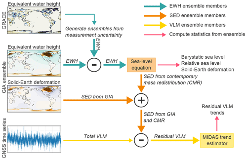
Figure 1 Overview of the processing steps taken to compute trends in residual VLM from the GRACE observations, GNSS time series, and GIA estimates. Thick arrows denote ensemble computations, while thin lines denote non-ensemble steps.

2.1 GIA estimates

GIA causes changes in the gravitational potential observed by GRACE satellites, causes SED which affects VLM observed by GNSS stations, and causes local RSL changes, which are observed by tide gauges (Tamisiea, 2011). To correct all these observations in a consistent way and to derive robust uncertainties, we use the ensemble of GIA estimates from C18, which provides a large ensemble of predictions, computed from varying the solid-Earth parameters and the ice-sheet histories. Each ensemble member comes with a likelihood that reflects its fitness to a global dataset of vertical GNSS velocities and sea-level paleorecords. Note that some circular reasoning is introduced here, as GNSS data were used to benchmark the GIA estimates. However, since the vast majority of the benchmark data comes from paleoindicators, and the cost function used to compute the likelihood is much more sensitive to paleodata rather than GNSS data, the impact of this at first glance circular reasoning on the results is limited. From this ensemble, we derive the mean and associated uncertainties for GIA-induced changes. We use a subset of 5000 ensemble members from the original set that contains 128 000 GIA estimates. This number is sufficient to approach the original ensemble set with a maximum deviation of 2.5 % from the original covariance matrix. Each ensemble member provides an estimate of the GIA effect on the gravitational potential, which we express in units of equivalent water height (EWH), an estimate of the solid-Earth deformation, and an estimate of the RSL changes.

To derive mean values and associated uncertainties from the ensemble, we use the likelihood ℒ of each ensemble member. We can then compute the mean value T_μ and its uncertainty T_σ for the process of interest as follows:

$$\begin{array}{ll}{\displaystyle }{T}_{\mathit{\mu }}& {\displaystyle }=\sum _{n=\mathrm{1}}^N{\displaystyle \frac{\mathcal{L}\left(n\right)}{{\sum }_{n=\mathrm{1}}^N\mathcal{L}\left(n\right)}}T\left(n\right),\\ {\displaystyle }{T}_{\mathit{\sigma }}& {\displaystyle }=\sqrt{\sum _{n=\mathrm{1}}^N{\displaystyle \frac{\mathcal{L}\left(n\right)}{{\sum }_{n=\mathrm{1}}^N\mathcal{L}\left(n\right)}}{\left(T\left(n\right)-T_{\mathit{\mu }}\right)}^{\mathrm{2}}},\end{array}$$

where N is the number of ensemble members and T(n) the value of the individual ensemble member. All uncertainties are on the 1σ level, unless otherwise specified. Note that the underlying probability density function (PDF) does not have to be Gaussian or symmetric. We can also derive an empirical PDF from the ensemble, from which confidence intervals at any level can be computed. To compute the empirical PDF, we first sort the values from low to high. Then we define 20 bins between the 1st and 99th percentiles of these values and compute the sum of the likelihood of all ensemble members that fall within each bin. The number of 20 bins is chosen as a trade-off between resolution and sample size. The linear trends in the ensemble-mean EWH, SED, and RSL with their uncertainty estimates are shown in Fig. 2.

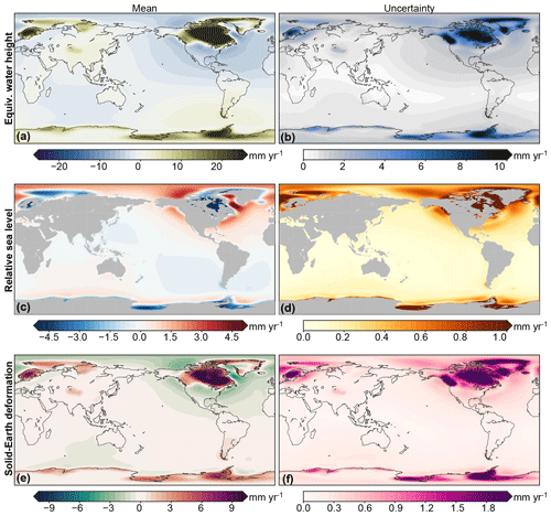
Figure 2 The effects of GIA on contemporary linear trends in EWH (a, b), RSL (c, d), and SED (e, f) as estimated from the 5000-member ensemble. The left panels show the ensemble mean and the right panels the 1σ uncertainty.

The regions with the largest trends and uncertainties are around the former ice sheets, while the far-field trends and uncertainties are smaller.

2.2 GRACE estimates of contemporary mass redistribution

To estimate contemporary mass redistribution, we use the JPL GRACE Release 6 (RL06) mass concentration (mascon) solution (Watkins et al., 2015). This solution provides monthly-mean estimates of EWH anomalies from March 2002 until June 2017, with some gaps at the beginning and end of the GRACE record and has a nominal spatial resolution of 3^∘ by 3^∘. We only look into mass changes on land, and we do not take ocean-bottom pressure changes driven by ocean dynamics into account, since its spatial variations are much smaller than the land mass changes (e.g., Watkins et al., 2015). For mascons that contain a coastline, a coastline resolution improvement (CRI) filter has been used to prevent the leakage of gravity signals between land and ocean, which leads to a better spatial representation of mass changes in coastal regions (Wiese et al., 2016). The RL06 solution comes with an estimate of the measurement uncertainty in the EWH changes in each mascon.

We first restore the original GIA correction applied to the GRACE solution and then we generate a 5000-member ensemble of GRACE EWH estimates, each perturbed randomly using the measurement uncertainty estimate in each mascon. These uncertainties are based on the formal error covariance matrix of the GRACE solutions; see Wiese et al. (2016) for details. This measurement uncertainty is given for each individual mascon and time step, and we assume that these uncertainties are uncorrelated in space and time. We then correct each perturbed mascon for GIA using one of the GIA ensemble members. Following Tamisiea (2011), we adjust the degree-2 order-1 terms of the GIA estimates to account for the fact that GRACE observations are taken from an inertial reference frame and not from the rotating Earth.

With this procedure, we now have 5000 estimates of contemporary mass redistribution, from which we derive the expected contemporary mass redistribution and the associated uncertainty, as well as the total land mass change. Note that the uncertainty estimates of these trends are only based on the spread in the ensemble and not on the uncertainty that arises from fitting a linear trend to the data. Since geophysical time series often exhibit serial correlation, this assumption results in an underestimation of the uncertainty in the resulting trends (Williams et al., 2014). Figure 3 shows the trends and associated uncertainties in the GRACE estimates. The uncertainty in the trend is dominated by the GIA uncertainty, as the spatial pattern is almost identical to the pattern shown in Fig. 2b, and the measurement uncertainties only reach values of about 1 mm yr⁻¹ EWH.

Figure 3 Trends and accompanying uncertainties in contemporary EWH changes on land over 2002–2017, observed by GRACE. These trends have been corrected for GIA.

To isolate the role of cryospheric and hydrologic processes, we separate the observed EWH changes into changes from the Greenland Ice Sheet, the Antarctic Ice Sheet, glaciers, and TWS. The EWH changes on both ice sheets can be isolated by only selecting the mascons that cover ice sheets. Glaciers tend to be smaller in size than ice sheets and glaciers often do not form the dominant source of mass redistribution in the mascons that contain glaciated regions. Therefore we cannot directly apply the separation per mascon. Instead, we use a similar approach as Reager et al. (2016). First, we determine those mascons that contain glaciated regions, based on the Randolph Glacier Inventory (Pfeffer et al., 2014). For mascons that do not overlap with a glaciated region, all mass changes are attributed to TWS changes. For the mascons that do contain glaciers, we distinguish three cases:

1. Mass changes from the peripheral glaciers of Greenland and Antarctica are part of the mass balance of both ice sheets.

2. For glaciers in Alaska, Arctic Canada, Iceland, Svalbard, the Russian Arctic, and the Southern Andes, we assume that the mass changes in the associated mascons are solely caused by glacier mass changes.

3. For all other glaciated regions, we use the annual glacier mass balance estimates based on geodetic and glaciological measurements from Zemp et al. (2019) as the glacier mass change estimate. We then subtract this glacier contribution from the total mass change in the mascon to obtain the TWS estimate. The annual estimates from Zemp et al. (2019) come with an estimate of the uncertainty. To propagate this uncertainty into the glacier and TWS mass balances, we perturb the annual glacier mass balance estimates for each ensemble member. Note that, contrary to Reager et al. (2016), we use the in situ estimates for the glaciers and ice caps in the high-mountain Asia region, instead of the estimates from Gardner et al. (2013), since the latter only cover the period 2003–2009, which would require an extrapolation of 8 years.

Figure 4 gives an overview of the mascon geometry and shows the mapping of each mascon into the individual processes.

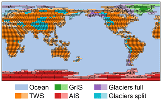
Figure 4 Overview of the GRACE mascon geometry and mascons associated with Greenland Ice Sheet (GrIS), Antarctic Ice Sheet (AIS), glaciers, and TWS mass changes. The light-colored mascons denote mascons which partially cover oceans and use the CRI filter. Mass changes in purple mascons (glaciers full) are fully attributed to glaciers, while turquoise mascons (glaciers split) are separated into a glacier and TWS term; see text for details.

2.3 Solid-Earth deformation and relative sea-level changes resulting from mass redistribution

The aforementioned procedure results in an ensemble of 5000 estimates of monthly land mass changes. To compute the resulting SED and RSL changes, we solve the sea-level equation (Clark and Lingle, 1977) for each ensemble member. We use the pseudo-spectral approach (Tamisiea et al., 2010), which requires the land mass changes to be transformed into spherical harmonics. We apply this transformation using the SHTns library (Schaeffer, 2013) up to degree and order 180. We solve the sea-level equation in the center-of-mass reference frame and apply the rotational feedback (Milne and Mitrovica, 1998). We assume that the solid-Earth response to contemporary mass redistribution is purely elastic and thus differs from viscoelastic GIA. We use the elastic Love numbers from Wang et al. (2012), which are based on the Preliminary Referenced Earth Model (PREM; Dziewonski and Anderson, 1981). This procedure results in an ensemble of 5000 estimates of local SED and RSL at each GRACE time step.

2.4 GNSS stations and VLM trend estimates

We use the GNSS dataset from the University of Nevada, Reno (Blewitt et al., 2018, http://geodesy.unr.edu, last access: 25 July 2019), which provides processed daily time series of over 14 000 permanent GNSS receivers in the ITRF2008 reference frame. For consistency, we only use observations that overlap with the GRACE era (2002–2017). We remove stations for which fewer than 1825 daily observations that overlap with the GRACE era (2002–2017) are available, which corresponds to a minimum record length of 5 years. This requirement, which is a trade-off between accuracy and data availability, results in a total of 8228 stations. Figure 5 shows a histogram of the record length per station, both before and after removing the observations that fall outside of the GRACE era.

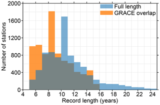
Figure 5 Histogram of the record length per station. Shown are all stations that fit the criteria outlined in Sect. 2.4. The blue bars show the record length before removing data outside the GRACE time span, and orange bars show the record length after removing data.

The histogram shows that most GNSS stations have a record length of around 8 to 10 years, or about half the length of the GRACE time span. Only a small fraction of the GNSS stations cover the full GRACE era. Since we only consider the observations within the GRACE era, not all data can be used, which results in a decrease in the record length that is available for some stations. We interpolate the monthly VLM that results from SED due to contemporary mass redistribution and GIA on the GNSS time steps, which enables us to separate the full GNSS time series into its components and the residual VLM following Eq. (3).

To estimate linear trends in the observed and residual height anomalies, we apply the MIDAS robust trend estimator (Blewitt et al., 2016) to the observed and residual height anomalies. The MIDAS estimator does not compute the linear trend using linear least squares but is based on the median of the height difference of each pair of anomalies that are separated by 1 year, while the uncertainty estimate is based on the standard deviation of the 1-year-separated anomaly differences. This approach has two advantages over the classical approach: it is less sensitive to discontinuities in the time series, which are omnipresent in GNSS records (Gazeaux et al., 2013), and it is computationally less expensive than least-squares estimation using an appropriate serially correlated noise model. To propagate the SED uncertainty into the residual VLM trends, we estimate the MIDAS trends for each ensemble member and GNSS station, which results in two sources of uncertainty: the spread in the residual VLM trends due to SED and the uncertainty that results from estimating linear trends from noisy GNSS data. We assume that the uncertainty from the trend estimator and the ensemble spread are independent, and these terms are added up in quadrature to obtain the final uncertainty.

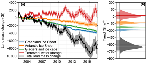
Figure 6 Total land mass changes as observed by GRACE, corrected for GIA. Panel (a) shows the expectation (thick line) and 90 % confidence intervals (shade) of the mass change time series for each process and the total land mass change. Negative values denote land mass loss. Panel (b) shows the expected value (thick line), 90 % confidence interval (left shade), and PDF (right shade) of the resulting linear trend.

3 Results

3.1 Global-mean land mass changes

The global-mean land mass changes due to contemporary mass redistribution are shown in Fig. 6 and Table 1, which show that all cryospheric processes cause a net land mass loss while TWS does not show a significant positive or negative linear trend. Over the first decade of the GRACE era, a positive TWS term has been observed by Reager et al. (2016) and Rietbroek et al. (2016), although the land mass loss over the last few years of the GRACE record has resulted in a trend that does not deviate significantly from zero. For all cryospheric processes, the total mass changes are dominated by the trend, and the variability around the longer-term trend is relatively small compared to TWS, whose interannual variability around the mean trend is substantial, especially after 2010. It is known that TWS exhibits substantial decadal and multidecadal variability (Humphrey et al., 2017; Wada et al., 2017), and a large part of this variability corresponds to the strong El Niño–Southern Oscillation cycles during this period, which are known to have a large effect on water stored on land (Boening et al., 2012; Fasullo et al., 2013).

The uncertainties in the trend and time series for Greenland and glaciers are smaller than the uncertainties for Antarctica and TWS. This difference is caused by the uncertainty in the GIA contribution, which is small for Greenland and most glaciated regions, while the GIA contribution is larger and more uncertain for the Antarctic Ice Sheet. The uncertainty in the TWS term is largely caused by the uncertainty in the GIA contribution from the former Laurentide Ice Sheet, which covered large parts of North America (see Fig. 3). Due to this uncertainty, the partitioning of the observed EWH changes over North America between GIA and contemporary changes is uncertain, which leads to a large spread in the possible TWS contribution from this region. The distributions shown in Fig. 6 are not symmetric, which causes slightly skewed confidence intervals in Table 1. The total land mass loss over the second half of the record is larger than the loss over the first half, which is caused by the accelerating contributions from Greenland and Antarctica and the slowdown of the TWS contribution. The trends in the individual terms are consistent with recent studies (Bamber et al., 2018; The IMBIE team, 2018), although quantifying TWS changes without GRACE is still challenging (Scanlon et al., 2018), which still hinders the validation of GRACE-based TWS changes.

Table 1 Trends in land mass changes and corresponding barystatic sea-level changes. The numbers in brackets show the uncertainties expressed as the corresponding 5 %–95 % confidence intervals. A positive sign for the mass change correspond to an increase in the mass on land, and a positive sign of the barystatic trend denotes a global-mean sea-level rise.

3.2 Local patterns in relative sea level and solid-Earth deformation

As discussed in Sect. 2.3, the mass changes will lead to local RSL and SED patterns. Figure 7 shows the resulting trends in local RSL with the accompanying uncertainty.

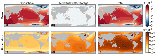
Figure 7 Trends in RSL resulting from mass redistribution observed by GRACE, separated into the cryosphere contribution (sum of glacier and ice sheet contribution), the TWS contribution, and the total land mass contribution. The trends have been computed over the full GRACE time span (2002–2017). Panels (a)–(c) show the mean trend, and panels (d)–(f) show the uncertainty.

As expected from the barystatic contribution (Fig. 6), the RSL trends are dominated by cryospheric processes, while the TWS-induced RSL trend is generally no more than a few tenths of millimeters per year and has a less pronounced spatial pattern. The local uncertainties are dominated by the TWS contribution. For large parts of the ocean, the uncertainty in the TWS contribution has a similar magnitude as the trend. The uncertainty in cryosphere-induced local RSL changes is limited to about 0.1 mm yr⁻¹, except for regions very close to glaciers and the ice sheets. The uncertainty in the total signal is again on the order of 0.1–0.2 mm yr⁻¹, which is substantially smaller than the signal itself.

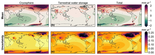
Figure 8 Trends in SED resulting from mass redistribution observed by GRACE, separated into the cryosphere contribution (sum of glacier and ice sheet contribution), the TWS contribution, and the total land mass contribution. The trends have been computed over the full GRACE time span (2002–2017). Panels (a)–(c) show the mean trend, and panels (d)–(f) show the uncertainty.

Figure 8 shows that, next to uplift at locations where the ice mass loss takes place, mass changes in the cryosphere result in some far-field SED signals, including subsidence of about 0.5 mm yr⁻¹ around Australia, and an uplift signal with a similar magnitude in Europe and northern Asia. TWS changes cause considerable near-field SED trends, e.g., in South America and Asia. Both uplift and subsidence occur, which shows that the barystatic trend consists of the sum of regions of land mass loss and land mass gain, and as such the TWS-induced SED signals, which have a predominantly near-field signature, will likely not follow the variability in the barystatic contribution from TWS. The SED uncertainty is large close to former glaciated regions due to the local impact of GIA. For other regions, the uncertainty is below the 0.1 mm yr⁻¹ level, also for the locations for which the local trend is large.

The TWS-induced total land mass change shows substantial temporal variability, and the mass loss at both the Greenland and Antarctic ice sheets is accelerating. Therefore, linear RSL and SED trends derived over a subset of the GRACE period are likely to deviate from the trends derived over the full period. As an example of the size of these deviations, Fig. 9 shows the linear RSL and SED trends over the first and second halves of the GRACE era, both covering 7.5 years.

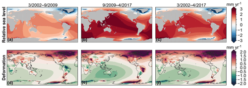
Figure 9 Trends in RSL (a–c) and SED (d–f) resulting from the total mass redistribution observed by GRACE over the first half (a, d), second half (b, e) of the GRACE observation, and the total GRACE period (c, f). Note that SED related to GIA is not included here.

As a result of the accelerating barystatic sea-level trends, the local RSL trends are overall larger during the second half of the GRACE era, although the spatial pattern only shows limited changes between the different periods. In contrast, local SED trends, mostly associated with TWS changes, show vast differences between both periods. Notable regions include the Amazon Basin and southern Africa, which subside over the first half of the period and show uplift over the second half of the GRACE period. The opposite occurs in the Rio de la Plata basin and northwest Australia. Linear trends in SED thus do depend on the time span over which these trends are computed, which implies that due to SED extrapolating a linear trend in VLM will cause biases.

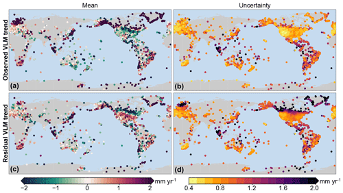
Figure 10 Observed VLM and residual VLM trends from GNSS records. (a, b) The trend in observed VLM and associated uncertainty. (c, d) Trends in residual VLM after removing the SED effects due to GIA and contemporary mass redistribution. All trends have been computed over the time spans for which GNSS and GRACE observations overlap.

3.3 The role of solid-Earth deformation in observed VLM trends

The linear trends in GNSS records (Fig. 10a) do show substantial spatial variability, even for nearby stations, although the uncertainty, which generally exceeds 0.5 mm yr⁻¹ due to the short GNSS records, noisy data, and the presence of jumps in the data (Williams, 2003), should be considered when comparing nearby stations. Nevertheless, the observed VLM trends show many well-known large-scale features, mostly associated with GIA and uplift associated with contemporary ice mass loss. To quantify the role of SED in actual VLM trends as observed by GNSS stations, we computed the linear SED trends over the time span of each GNSS station (Fig. 11).

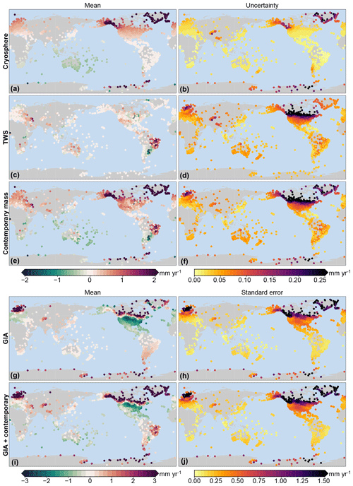
Figure 11 The modeled linear trends due to SED computed over the time span of the individual GNSS record. The left panels show the mean trend, and the right panels show the uncertainty from the large ensemble. Note that the color scales for the top three rows differ from the color scales of the bottom two rows.

The cryosphere-driven SED trends mostly show smooth spatial variations, and compared to the trend the interannual variations are small, which implies that the specific time span of the GNSS record has a limited impact on the observed linear trend in SED. Cryosphere-induced SED results in linear trends of a few tenths of a millimeter per year or larger at many GNSS stations. These trends not only reflect the well-known near-field uplift signals at or near the ice mass loss locations, which dominate the VLM signal for many regions where ice mass loss occurs, but also in the far field, with notable uplift in large parts of Europe and the US and subsidence in Australia. The uncertainty in these trends is negligibly small, except for the stations close to the locations of ice mass loss.

In contrast, the TWS-induced SED trends show a less smooth pattern: sharp contrasts in the trends between nearby stations can, for example, be seen in North America and South America, owing to the aforementioned difference in the time span of the GNSS records and the TWS trends that depend on the period over which these trends are computed. SED trends at coastal locations can be substantial, which points at possible biases when VLM estimates used to correct tide-gauge observations do not account for TWS-induced SED. For many regions, the SED trend is dominated by GIA, especially for the northeastern parts of North America and northern Europe, while for South America and Australia contemporary mass redistribution is the dominant SED component. Not only the SED trends but also the associated uncertainties are mostly driven by the GIA. Outside regions with a notable GIA signal, the uncertainties in the trends are small.

The removal of all modeled SED signals (Fig. 10c) highlights regional differences: for Europe, Australia, and South America, SED explains a large part of the observed large-scale VLM features, while for North America a different pattern emerges, with an uplift signal over large parts of the United States. This uplift could have its cause in the GIA estimates: the ensemble mean predicts a substantial subsidence pattern over large parts of North America, associated with the collapse of the Laurentide forebulge (Fig. 2e), which is stronger than projected from some other models, such as ICE6G-VM5a (Peltier et al., 2015). For most cryospheric regions, the trends change, but a substantial residual signal remains. A possible explanation for this large residual is the fact that both the GIA estimates and the GRACE observations provide contemporary mass redistribution estimates at relatively coarse spatial resolutions, while it is known that SED induced by GIA and contemporary ice mass loss can have a very local character in these regions due to localized mass changes and complex Earth structures (e.g., Khan et al., 2010; Hay et al., 2017). Some large-scale VLM features visible in the GNSS trends cannot be explained by the modeled SED. For some regions, such as Japan and Chile, tectonic activity is a likely candidate, but the uplift in southern Africa is unlikely to be tectonic in nature. Nevertheless, the scatter plot in Fig. 12 shows that the SED trend for most stations is close to the observed VLM trend, although there are multiple stations that show large trends that are not explained by the model. Given the fact that many relevant local processes, such as tectonics and local subsidence, are still present in the residual VLM trend, these outliers are not surprising.

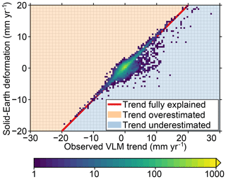
Figure 12 Scatter plot of observed VLM trends (Fig. 10a) versus the trend in SED resulting from GIA and contemporary mass redistribution (Fig. 11i). The color denotes the number of stations for each trend pair within 0.5 mm yr⁻¹. For points on the red line, the observed VLM trend and SED trend agree completely; in the orange area, the SED trend is larger than the observed VLM trend; for the blue area, the SED trend is smaller than the observed VLM trend.

The mean linear trend for all 8166 stations is 0.34 mm yr⁻¹ with a standard deviation of 4.46 mm yr⁻¹, while the mean residual trend is 0.44 mm yr⁻¹ with a standard deviation of 4.28 mm yr⁻¹. The coefficient of determination (R²) of the modeled trends is just 7.5 %. The full list of stations also contains many stations for which the MIDAS estimates very large uncertainties, sometimes exceeding 10 mm yr⁻¹. If we limit our station selection to those stations for which the uncertainty in the observed VLM trend is smaller than 1 mm yr⁻¹, which is the case for 4252 out of 8166 stations, we obtain a coefficient of determination of 34 % and a reduction of the standard deviation from 2.30 to 1.86 mm yr⁻¹.

3.4 Solid-Earth deformation and long tide-gauge records

To demonstrate the impact of SED on tide-gauge observations, we revisit the analysis by Thompson et al. (T16; 2016). In this study, linear trends from a set of 15 long-term tide-gauge records are compared to multiple recent global-mean sea-level reconstructions. A discrepancy was found between the long tide-gauge records and most reconstructions, including the recent reconstructions from Hay et al. (2015) and Dangendorf et al. (2017). This study did not use GNSS observations to correct tide gauges for local VLM. Here, we determine whether observed and residual VLM explain a part of this discrepancy.

For many of these stations, long VLM records from nearby GNSS stations are available. Some stations from that study are not in the vicinity (i.e., more than 50 km) of any GNSS station with a long record, or the combination of VLM and the tide-gauge trend results in an unrealistically low sea-level trend. We have removed these stations and added nearby stations as a replacement where possible. Text S1 in the Supplement gives an overview of the stations that differ from T16 with an explanation of the reason, and Table S1 in the Supplement lists all tide-gauge stations together with the GNSS stations used to determine the local VLM trends. The linear trends in local sea level have been computed from annual tide-gauge data obtained from the Permanent Service for Mean Sea Level (PSMSL, 2018; Holgate et al., 2013) using the Hector software (Bos et al., 2013) while assuming a power-law spectrum for the temporally correlated noise in each tide-gauge record. To stay consistent with T16, we only use annual tide-gauge data from 1901 to 2000.

We compute linear trends in the uncorrected tide-gauge record, and we compute the trend by applying three different correction models. In the “GIA-removed” model, the ensemble-mean GIA RSL trend is removed from the tide-gauge trend. For the “VLM-removed” model, the observed VLM trend is removed from the tide-gauge trend. Both the GIA-removed and the VLM-removed models are commonly used as a correction to tide-gauge observations (e.g., Wöppelmann et al., 2009). In the full model, we remove both the residual VLM trend and the GIA RSL trend. The full model removes the spatial variations due to GIA and local VLM not related to SED, while it avoids the extrapolation of the nonlinear SED signal due to contemporary mass redistribution. In the full model, sea-floor deformation signals due to contemporary mass redistribution and GIA are also retained in tide-gauge records. The uncertainties in the VLM and GIA estimates are derived from the ensemble and subsequently added in quadrature to the uncertainty in the linear trend from the tide-gauge record. Figure 13 shows the resulting linear trends at each station. For comparison, we also computed the trends for the GIA-removed and full models using the ICE6G-D VM5a model (Peltier et al., 2018), which is an updated version of the ICE6G-C VM5a GIA model (Peltier et al., 2015) used in T16.

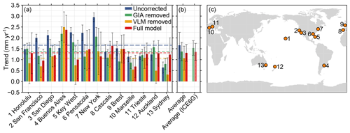
Figure 13 The effect of vertical land motion on 20th-century linear trends in tide-gauge records. (a) Linear trends in long tide-gauge records (1901–2000), with various correction models applied for vertical land motion. Blue: no correction, green: GIA RSL removed, yellow: observed VLM trend removed, and red: GIA and residual VLM trend removed. The dashed lines show the median trends for each correction, which are also depicted in panel (b). The error bars in panel (b) denote the inter-station standard deviations of the trends for each model. Panel (c) shows the locations of the tide gauges. The black bars denote the 1σ uncertainties.

From the individual trends, we computed the mean and the inter-station spread, which we express as the standard deviation between the trends from each tide-gauge station (Fig. 13). All correction models reduce the spread between the stations, compared to the uncorrected trends. Removing the observed VLM trends from the tide-gauge trends also reduces the inter-station spread in the trends, although to a lesser extent than the GIA-removed model. All three correction models do reduce the station-mean trend from the 1.7 mm yr⁻¹ in the uncorrected model. The VLM-removed model has the lowest mean trend (1.1 mm yr⁻¹), but this correction suffers from the two aforementioned problems: the linear trend due to SED over the GNSS record is not representative of the full tide-gauge record and the sea-floor deformation signal is removed from the tide-gauge data. The latter effect explains the low mean trend for this method as over the last few decades, due to contemporary mass redistribution, the sea floor has subsided by about 0.1 mm yr⁻¹ (Frederikse et al., 2017), which would result in an underestimation of GMSL if sea-floor deformation is not taken into account. The full model results in a station-average trend of 1.3 mm yr⁻¹, which lies in between the GIA-removed and VLM-removed models, but overall with the lowest inter-station spread. The mean trend of the full model is close to the trend found by Hay et al. (2015) and Dangendorf et al. (2017), who find a mean trend of 1.3 and 1.2 mm yr⁻¹, respectively, over the 20th century. When we correct the tide-gauge records for GIA using the ICE6G-D model, we find a station-mean trend of 1.5 mm yr⁻¹, which is close to the trend found by T16. The difference between C18 and ICE6G-D points at the impact of the uncertainty in GIA models on tide-gauge trends. When we compare the full correction models, the difference between C18 and ICE6G-D again becomes much smaller, which shows that the residual VLM trend partially offsets the uncertainty in GIA estimates. Note that T16 also argues that averaging the linear trend in sea level from these long tide-gauge data likely underestimates the global-mean sea-level trend due to the spatial patterns associated with ice mass loss and ocean dynamics. Here, we do not consider this spatial sampling bias, so the gap between the long tide-gauge records and global-mean sea-level reconstructions discussed by T16 cannot yet be fully reconciled from these results.

4 Conclusions

We have developed an alternative approach to correct tide gauges for local VLM that reduces the aliasing of decadal and multidecadal variability in contemporary mass redistribution into VLM trend estimates from short GNSS records. This method also avoids the bias when global-mean sea-level changes are estimated from geocentric sea-level observations.

The local solid-Earth deformation signal due to contemporary mass redistribution depends on the location and the time span. Mass changes from ice sheets and glaciers cause large-scale deformation patterns, with far-field deformation patterns reaching values on the order of 0.5 mm yr⁻¹. TWS changes cause substantial local SED trends, especially when computed over a subset of the whole GRACE time span. The SED trends computed over the GNSS record time spans can reach values of more than 1 mm yr⁻¹, not only near melting ice sheets but also in regions where large TWS changes occur, such as the Amazon Basin.

This solid-Earth deformation resulting from GIA and contemporary mass redistribution explains a substantial part of the observed GNSS trends: for all 8166 stations, we obtain a coefficient of determination of 7.5 %. When we only consider stations for which the standard error in the observed VLM trend is smaller than 1 mm yr⁻¹, the coefficient of determination becomes 34 %. This difference suggests that a nonnegligible part of the residual VLM trends can be attributed to the uncertainty in the estimated linear trends in VLM from noisy GNSS data, and that the uncertainties should not be overlooked when applying the observed and residual VLM trends to tide-gauge data. In multiple regions, including South America, Australia, and Europe, large-scale patterns of observed VLM trends are explained by solid-Earth deformation related to cryospheric and hydrological processes. In contrast, we note that for some regions, such as North America, the removal results in the appearance of substantial residual trends. A likely candidate for this residual trend is unquantified uncertainty in the GIA term: the global model that we use does not account for lateral variations in the mantle viscosity structure and is not optimized for a specific region, and uncertainties in the deglaciation history that are not fully represented in the GIA ensemble could lead to an underestimation of the uncertainty in formerly glaciated regions.

VLM trends derived over the GNSS record length can be substantially affected by contemporary mass redistribution variability, which causes biases when these trends are extrapolated to explain VLM over longer tide-gauge records. This bias affects global and regional sea-level reconstructions and projections that depend on VLM-corrected tide gauges. VLM estimates derived from differences between satellite altimetry and tide-gauge observations (Wöppelmann and Marcos, 2016; Kleinherenbrink et al., 2018) are also affected by this bias. Correcting tide-gauge observations with the residual VLM trends instead of observed VLM trends avoids this source of bias. For a set of long tide-gauge records, correcting tide gauges using the residual VLM trends not only results in a smaller spread between stations but also reduces the gap between the long-term trend at these stations and trends found in recent global-mean sea-level reconstructions that was found by Thompson et al. (2016). Note that we have only applied our method to a limited subset of tide gauges, which means that the reduction in local sea-level trends and the spread among stations is not necessarily representative of other tide gauges. Whether correcting tide gauges using our method affects global sea-level reconstructions is therefore still an unanswered question.

This approach comes with multiple limitations. The GRACE solutions have limited temporal and spatial resolutions: since the observations only cover the period 2002–2017, GNSS observations from outside the GRACE period have been discarded, which, for some stations, substantially shortens the records, as displayed in Fig. 5. This limitation means that the results of this study can be improved if SED estimates are expanded to cover the full GNSS record. Models of mass redistribution could be used for this purpose. While for ice mass changes model results show good agreements with observations, model estimates of TWS changes are still less reliable than GRACE observations (Scanlon et al., 2018), which in turn limits the ability to use models to estimate SED. Due to the coarse spatial resolution of the GRACE data, sharp gradients in mass redistribution are smeared out over larger areas. Since SED is sensitive to these local mass changes, the SED computed here could underestimate local SED in regions with strong spatial gradients. This issue could be one of the reasons of the unexplained residual land motion around Greenland, Antarctica, and Alaska visible in Fig. 10c. Another limitation is that we compute SED with an elastic model that assumes a laterally uniform Earth structure. In some regions, such as West Antarctica, elastic properties can deviate from their global-mean values and viscoelastic effects could occur on decadal timescales, which leads to additional deformation on top of the elastic response (e.g., Hay et al., 2017).

Another important limitation is that we only consider the effects of solid-Earth deformation due to GIA and contemporary mass redistribution, while many other local and large-scale processes, such as tectonics and local subsidence due to groundwater and hydrocarbon extraction, are still present in the residual VLM time series. Like SED, many of these processes are also highly nonlinear and therefore also cause problems when records are extrapolated. Therefore, the linear trend in residual VLM that we have computed cannot be regarded as the secular background trend that is free from any bias when extrapolated back in time. A full understanding of these processes is key to fully understanding the impact of vertical land motion on tide-gauge observations. We hope that the method presented here will serve as a base for future studies to further separate the observed VLM trends into individual components by integrating new models of physical processes.