the Creative Commons Attribution 4.0 License.
the Creative Commons Attribution 4.0 License.
 | 15 Nov 2019
Prediction of seismic P-wave velocity using machine learning
Ines Dumke
Measurements of seismic velocity as a function of depth are generally restricted to borehole locations and are therefore sparse in the world's oceans. Consequently, in the absence of measurements or suitable seismic data, studies requiring knowledge of seismic velocities often obtain these from simple empirical relationships. However, empirically derived velocities may be inaccurate, as they are typically limited to certain geological settings, and other parameters potentially influencing seismic velocities, such as depth to basement, crustal age, or heat flow, are not taken into account. Here, we present a machine learning approach to predict the overall trend of seismic P-wave velocity (vp) as a function of depth (z) for any marine location. Based on a training dataset consisting of vp(z) data from 333 boreholes and 38 geological and spatial predictors obtained from publicly available global datasets, a prediction model was created using the random forests method. In 60 % of the tested locations, the predicted seismic velocities were superior to those calculated empirically. The results indicate a promising potential for global prediction of vp(z) data, which will allow the improvement of geophysical models in areas lacking first-hand velocity data.
- Article
(7955 KB) - Full-text XML
- BibTeX
- EndNote


Seismic P-wave velocities (vp) and velocity–depth profiles are needed in many marine–geophysical applications, e.g. for seismic data processing, for time–depth conversions, or to estimate hydrate concentrations in gas hydrate modelling. Direct measurements of seismic velocities, however, are sparse and limited to borehole locations such as those drilled by the Deep Sea Drilling Project (DSDP), the Ocean Drilling Program (ODP), and the International Ocean Discovery Program (IODP).
Seismic velocities can also be obtained indirectly from seismic data. Approaches include derivation of 1-D velocity profiles via refraction seismology using ocean bottom seismometers (OBSs) (Bünz et al., 2005; Mienert et al., 2005; Westbrook et al., 2008; Plaza-Faverola et al., 2010a, b, 2014), and velocity analysis of large-offset reflection seismic data (Crutchley et al., 2010, 2014; Plaza-Faverola et al., 2012). However, suitable seismic datasets are only available in certain areas, and OBS-derived velocity profiles are of relatively low spatial and vertical resolution.
In the absence of measurements and refraction seismic data, constant velocities are often used for time–depth conversions (e.g. Brune et al., 2010) or processing of reflection seismic data (Crutchley et al., 2010, 2011, 2013; Netzeband et al., 2010; Krabbenhoeft et al., 2013; Dumke et al., 2014), even though a constant velocity–depth profile is generally unrealistic and will thus lead to inaccurate results.
As an alternative, empirical velocity functions have been derived, which are based on averaged measurements and provide seismic velocity–depth relationships for different geological and geographical settings. For example, Hamilton (1979, 1980, 1985) used averaged vp measurements from boreholes and sonobuoys to derive velocity–depth functions for different marine settings and sediment types. Velocities calculated from these empirical functions have been used, e.g., for time–depth conversions (Lilley et al., 1993; Brune et al., 2010), brute stack processing of reflection seismic data, as well as local (Bünz et al., 2005) and regional (Scanlon et al., 1996; Wang et al., 2014) velocity models.
Although velocity profiles calculated from empirical functions may work well in some cases, empirical functions do not always produce accurate vp(z) profiles, due to their use of depth as the only input parameter and their limitation to certain regions or geological settings. Mienert et al. (2005) observed both agreements and disagreements between velocity profiles derived from OBS data and calculated from Hamilton functions, whereas Westbrook et al. (2008) argue that empirical functions are in general not representative of other areas due to variations in lithology and compaction history. Moreover, the Hamilton functions fail to provide correct velocities in areas containing gas hydrates or gas-saturated sediments (Bünz et al., 2005; Westbrook et al., 2008). Consequently, an alternative method is required to estimate vp(z) profiles for a larger variety of geological settings.
Over the last years, parameters in many different applications have been successfully predicted using machine learning techniques (e.g. Lary et al., 2016). In geosciences and remote sensing, machine learning methods have been used to predict soil properties (Gasch et al., 2015; Ließ et al., 2016; Meyer et al., 2018), air temperatures (Meyer et al., 2016a, 2018), biomass (Meyer et al., 2017), and the elasticity modulus of granitic rocks (Karakus, 2011). Applications also extended into marine settings, involving the prediction of sediment mud content off southwest Australia (Li et al., 2011), as well as parameters such as seafloor porosity (Martin et al., 2015; Wood et al., 2018), seafloor biomass (Wei et al., 2010), and seafloor total organic carbon (Wood et al., 2018; Lee et al., 2019) on a global scale. These studies were in general restricted to the prediction of one value per geographic location; the prediction of multiple values, such as depth profiles, has, to our knowledge, not been attempted before.
In machine learning, a prediction model is constructed from a training dataset consisting of the target variable to be predicted and a set of predictor variables. A random subset of the data, the test set, is typically held back for testing and validation of the prediction model. The most widely used machine learning methods include artificial neural networks (ANNs; e.g. Priddy and Keller, 2005), support vector machines (SVMs; Vapnik, 2000), and random forests (RFs; Breiman, 2001).
RF is an ensemble classifier based on the concept of decision trees, which are grown from the training set by randomly drawing a subset of samples with replacement (bagging or bootstrap approach) (Breiman, 2001). At each tree node, the data are split based on a random subset of predictor variables to partition the data into relatively homogeneous subsets and maximize the differences between the offspring branches. Each tree predicts on all samples in the test set and the final prediction is obtained by averaging the predictions from all trees.
RF has been repeatedly found to be superior to other machine learning methods. For example, Li et al. (2011) tested 23 machine learning algorithms – including RF, SVM, and kriging methods – to predict mud content in marine sediments and found that RF, along with RF combined with ordinary kriging or inverse distance squared, provided the best prediction results. Cracknell and Reading (2014) applied five machine learning methods to lithology classification of multispectral satellite data and reported higher classification accuracy for RF than for naive Bayes, SVM, ANN, and k-nearest neighbours. RF is robust to noise and outliers (Breiman, 2001), and it is also able to handle high-dimensional and complex data. Moreover, RF does not require any preprocessing of the input variables and provides variable importance measurements, making it the first-choice method in many applications.
Here, we apply RF to predict seismic P-wave velocity–depth profiles on a global scale, based on a set of 38 geological and spatial predictors that are freely available from global datasets. Prediction performance is evaluated and compared to velocity–depth profiles calculated from empirical vp functions. We also test additional methods for the improvement of model performance and determine which predictors are most important for the prediction of vp.
2.1 Dataset
2.1.1 vp(z) data
vp(z) profiles for training the RF model were obtained from boreholes drilled by the DSDP, ODP, and IODP campaigns between 1975 and 2016. All boreholes containing vp measurements were used, excluding those with bad-quality logs according to the logging description notes. In total, 333 boreholes were included in the dataset, the distribution of which is shown in Fig. 1. All vp(z) data from these boreholes are available through http://www.iodp.org (last access: 11 November 2019) and were downloaded from the archive at http://mlp.ldeo.columbia.edu/logdb/scientific_ocean_drilling/ (last access: 11 November 2019).
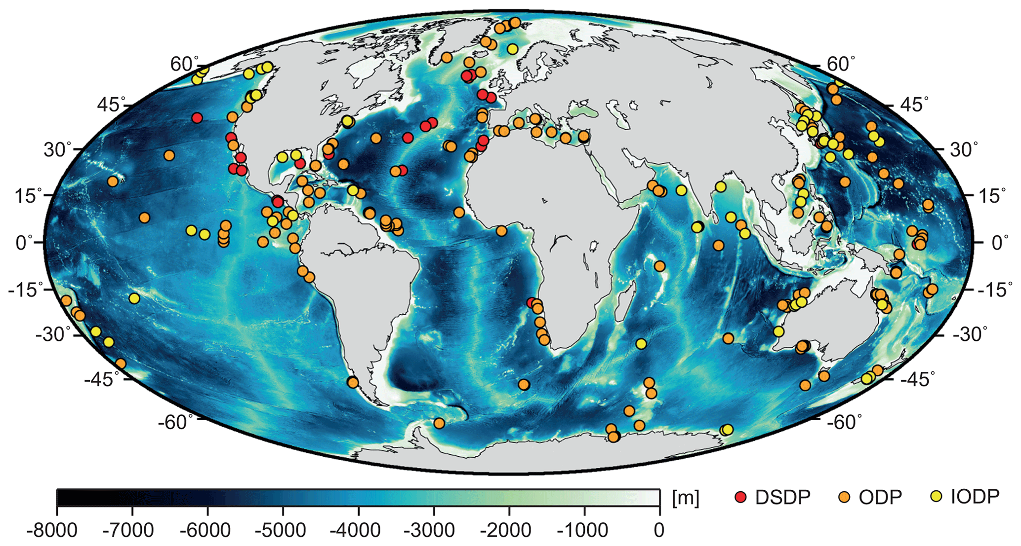
Figure 1Distribution of the 333 boreholes from which vp(z) profiles were extracted. DSDP: Deep Sea Drilling Project; ODP: Ocean Drilling Program; IODP: International Ocean Discovery Program. Bathymetry (30 s resolution) is from the GEBCO_2014 grid (http://www.gebco.net, last access: 11 November 2019).
A multitude of measuring methods and tools had been employed by the different drilling campaigns to obtain vp measurements, including wireline logging tools (e.g. sonic digital tool, long-spacing sonic tool, dipole sonic imager, borehole compensated sonic tool) and logging-while-drilling tools (sonicVISION tool, ideal sonic-while-drilling tool). The majority of these methods provided vp measurements at 0.15 m depth intervals. Lengths of the vp logs varied greatly, ranging between 10 and 1800 m (average: 370 m), with top depths of 0–1270 m (average: 138 m) and bottom depths of 16–2460 m (average: 508 m).
After exporting the vp(z) profiles for each borehole, the data were smoothed using a moving average filter with a window of 181 data points (corresponding to ca. 27 m for a 0.15 m depth interval). Smoothing was applied to remove outliers and to account for unknown and varying degrees of uncertainty associated with the different measurement tools. In addition, smoothing was expected to facilitate prediction, as the aim was to predict the general vp(z) trend at a given location, rather than predicting exact vp values at a certain depth. Following smoothing, the profiles were sampled to 5 m depth intervals, using the same depth steps in all boreholes.
2.1.2 Predictors
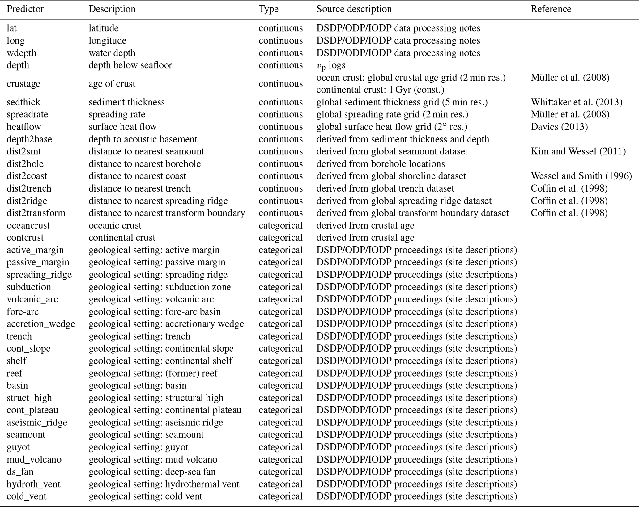
A total of 38 geological and spatial variables were included as predictors (Table 1). These predictors are parameters that were assumed to influence P-wave velocity. However, only predictors that could be obtained for each of the 333 borehole locations were used. Predictors such as latitude (lat), longitude (long), and water depth (wdepth) were taken from the borehole's metadata, whereas other predictors were extracted from freely available global datasets and grids (Table 1). In addition, predictors describing the borehole's geological setting were determined from the site descriptions given in the proceedings of each drilling campaign. Some parameters known to influence seismic velocity – e.g. porosity, density, or pressure – had to be left out as suitable datasets were not available. Although some of these parameters had been measured in DSDP, ODP, and IODP boreholes, they had not necessarily been logged at the same locations and depths at which vp data had been measured and therefore could not be obtained at all of the 333 boreholes used.
For predictor variables based on global grids, such as age of crust
(crustage), sediment thickness (sedthick), and surface heat flow (heatflow),
values were extracted for each borehole location in Generic Mapping Tools (GMT) (Wessel et al.,
2013), using the command grdtrack. As the crustal age grid (Müller et al., 2008)
contained only ages for oceanic crust, the age for locations above
continental crust was set to 1 billion years to represent a significantly
older age than that of oceanic crust. Depth to basement (depth2base) was
calculated by subtracting the depth values from the (constant) sedthick
value at each borehole location, so that depths below the basement were
indicated by a negative depth2base value. The distance predictor variables,
e.g. distance to the nearest seamount (dist2smt), were calculated based on
the borehole location and the respective datasets (Table 1) via the GMT
command mapproject.
Of the 38 predictors, 15 were of the type continuous, whereas 23 were categorical variables describing the type of crust and the geological setting at each borehole location (Table 1). The categorical predictors were encoded as either 0 or 1, depending on whether the predictor corresponded to the geological setting at a given borehole. Multiple categories were possible; for example, a borehole located in a fore-arc basin above continental crust would be described by 1 for the predictors “contcrust”, “active_margin”, “subduction”, and “fore-arc” and by 0 for all other categorical predictors. Across the categorical predictors, the number of boreholes for which a predictor was set to 1 varied between 2 (0.6 %) and 191 (57.4 %); on average, the geological setting described by a categorical predictor applied to 42 boreholes (12.7 %).
2.2 Random forest implementation
RF was implemented using the RandomForestRegressor in Python's machine learning library scikit-learn (Pedregosa et al., 2011). Two parameters needed to be set: the number of trees (n_estimators) and the number of randomly selected predictors to consider for splitting the data at each node (max_features). Many studies used 500 trees (e.g. Micheletti et al., 2014; Belgiu and Drăguţ, 2016; Meyer et al., 2017, 2018), but as performance still increased after 500 trees, we chose 1000 trees instead. The max_features parameter was initially set to all predictors (38), as recommended for regression cases (Pedregosa et al., 2011; Müller and Guido, 2017), although some studies suggest tuning this parameter to optimize model results (Micheletti et al., 2014; Ließ et al., 2016; Meyer et al., 2016b).
2.3 Model validation
A 10-fold cross validation (CV), an approach frequently used in model validation (e.g. Li et al., 2011; Gasch et al., 2015; Ließ et al., 2016; Meyer et al., 2016b, 2018), was applied to validate the RF model. CV involved partitioning the dataset into 10 equally sized folds. Nine of these folds acted as the training set used for model building, whereas the remaining fold was used for testing the model and evaluating the predictions. This procedure was repeated so that each fold acted once as the test fold, and hence each borehole was once part of the test set.
Partitioning into folds was not done randomly from all available data points but by applying a leave-location-out (LLO) approach (Gasch et al., 2015; Meyer et al., 2016a, 2018) in which the data remained separated into boreholes, i.e. locations, so that each fold contained 1∕10 of the boreholes. With 33–34 boreholes per fold, the size of the training dataset thus varied between 20 166 and 20 784 data points. By using the LLO approach, whole locations were left out of the training set, thereby allowing the RF model to be tested on unknown locations through prediction of vp for each borehole in the test fold. If the folds were chosen randomly from all data points, each borehole location would be represented in the training set by at least some data points, resulting in overoptimistic model performance due to spatial overfitting (Gasch et al., 2015; Meyer et al., 2016a, 2018).
Performance of the RF model was evaluated in two ways: (1) by standard error metrics and (2) by the proportion of boreholes with predicted vp(z) superior to that of empirical functions. The standard error metrics root mean square error (RMSE), mean absolute error (MAE), and the coefficient of determination (R2) were calculated based on the comparison of the predicted and true vp(z) curves for each borehole in the test fold. RMSE, MAE, and R2 of all test folds were then averaged to give final performance values.
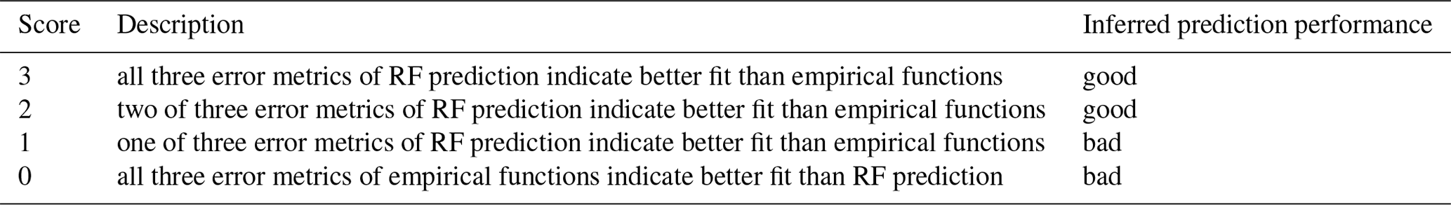
To determine the proportion of boreholes with better vp(z) trends than those from empirical functions, we tested how well the predicted vp(z) curves performed compared to vp(z) curves calculated from empirical functions. Using the depth values of the respective test borehole, vp(z) profiles were therefore calculated from the five empirical functions presented by Hamilton (1985) for deep-sea sediments, i.e. for terrigenous silt and clays (termed H1 in the following), terrigenous sediments (H2), siliceous sediments (H3), calcareous sediments (H4), and pelagic clay (H5). These vp functions were chosen because the deep-sea setting applied to the majority of the boreholes or was the best choice in the absence of empirical functions for other geological settings such as mid-ocean ridges. The resulting Hamilton curves were evaluated against the true vp(z) profile, and RMSE, MAE, and R2 were averaged over the five curves. The averaged error metrics were then compared to the error metrics of the prediction, and each borehole was assigned a score between 0 and 3 as shown in Table 2. Scores 2 and 3 were interpreted as a good prediction, i.e. better than the Hamilton curves, whereas scores 0 and 1 represented generally bad predictions. The proportion of boreholes with good predictions was then averaged over the 10 folds.
Table 2Scores for performance comparison between RF prediction and vp calculated from the empirical functions of Hamilton (1985).
2.4 Predictor selection
To determine the most important predictors for vp prediction, a predictor selection approach was performed. Although RF can deal with high data dimensionality, predictor selection is still recommended, not only to remove predictors that could cause overfitting but also to increase model performance (e.g. Belgiu and Drăguţ, 2016, and references therein). We applied recursive feature elimination (RFE), which is based on the variable importance scores provided by the RF algorithm. After calculating and evaluating a model with all 38 predictors, the least important predictor according to the variable importance scores was removed and the model was calculated again. This procedure was repeated until only one predictor was left. By evaluating model performance for each run via CV, using the same 10 folds as before, the optimum number of predictors was determined.
2.5 Tests to improve prediction performance
Additional tests to improve prediction performance included predictor scaling, variation of the max_features parameter, and stronger smoothing of the vp(z) curves. All models were evaluated via a 10-fold CV, using the same folds as in the previous model runs.
Predictor scaling was applied to account for the different data ranges of continuous and categorical features. Model performance may be negatively affected if different types of variables or data ranges are used (Otey et al., 2006; Strobl et al., 2007), even though RF does not normally require scaled input data. All continuous predictors were scaled to between 0 and 1 to match the range of the categorical predictors, and RFE was repeated.
As tuning of the max_features parameter, i.e. the number of predictors to consider at each split, is recommended by some studies (Ließ et al., 2016; Meyer et al., 2018), an additional model was run in which max_features was varied between 2 and 38 (all features) with an interval of 2. Performance was evaluated for each case to find the optimum number of predictors to choose from at each split.
A third attempt to improve model performance involved enhanced filtering of the vp(z) curves so that larger vp variations were smoothed out and the curves indicated only a general trend, which would likely be sufficient for many applications requiring knowledge of vp with depth. The vp curves therefore underwent spline smoothing using Python's scipy function UnivariateSpline. Three separate RF models were calculated: (i) spline1, which involved spline smoothing of the predicted curve of each test borehole; (ii) spline2, in which the input vp(z) data were smoothed; and (iii) spline3, where both the input vp(z) curves and the predictions were smoothed. All three cases were run with the 16 most important predictors as determined from the RFE results and compared to the previous models.
3.1 Prediction performance
Overall, many vp(z) profiles were predicted well by the RF models. For the 38-predictor CV, about 59.5 % of the boreholes had prediction scores of 2 or 3, representing a prediction performance superior to that of the Hamilton functions.
Predictions of prediction score 3, which were characterized by lower RMSE and MAE values and a higher R2 than the five empirical functions, often exhibited a good fit to the true vp(z) curve (Fig. 2a–d). Even for more complex velocity profiles, e.g. involving a velocity reduction at depth (Fig. 2d) or a strong increase such as that from 2.2 km s−1 to >4 km s−1 at the basement contact in Fig. 2b, the predicted vp(z) curves generally matched the true curves well. In some cases, score 3 predictions did not provide a good fit but still performed better than the empirical functions (Fig. 2e). Score 2 predictions generally indicated the correct trend of the true vp(z) profile (Fig. 2f), whereas score 1 and score 0 predictions failed to do so, with velocities often considerably higher or lower than the true velocities (Fig. 2g, h).
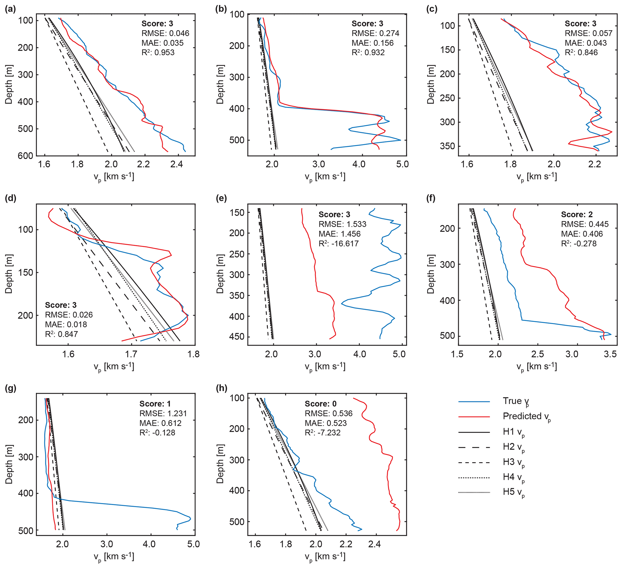
Figure 2Examples for true vp(z) curves, predicted vp(z) curves, and vp(z) calculated from the five Hamilton functions (Hamilton, 1985) used in model evaluation. Panels (a)–(d) shows well-predicted vp(z) curves of score 3, (e) lower-quality prediction of score 3, (f) score 2, and (g)–(h) bad predictions of scores 1 and 0. See Sect. 2.3 for a description of H1 to H5.
The RFE CV revealed best performance for 33 predictors, as indicated by the lowest RMSE and MAE values (Fig. 3a). The proportion of boreholes with prediction scores of 2 or 3 was 59.2 % and thus slightly lower than for the 38-predictor CV (59.5 %; Fig. 3b). The highest proportion of 61.9 % was achieved by the 16-predictor model (Fig. 3b), but this also led to the highest errors (Fig. 3a).
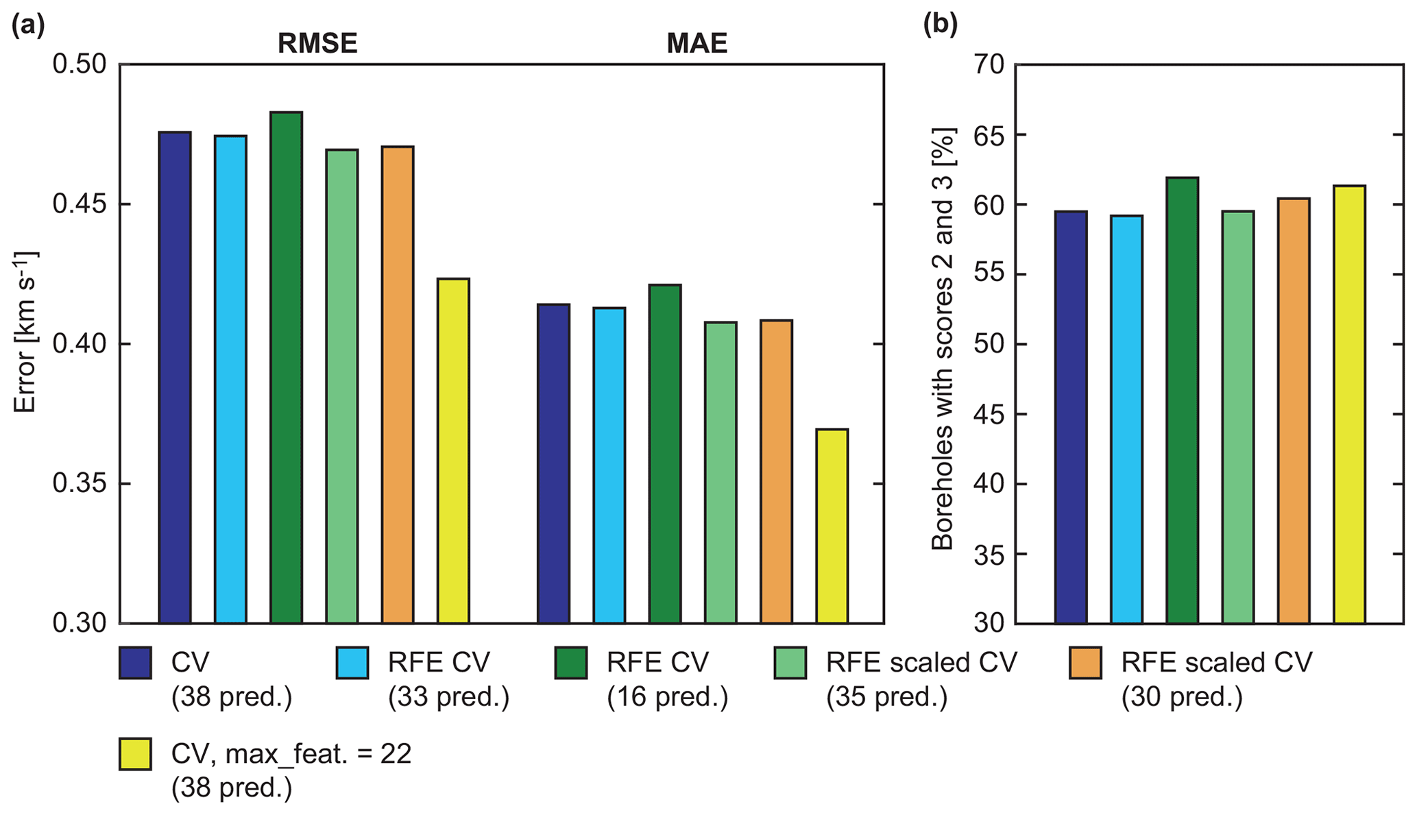
Figure 3Comparison of (a) error metrics and (b) proportion of well-predicted boreholes (scores 2 and 3) for different model runs. RMSE: root mean square error; MAE: mean absolute error; CV: cross validation; RFE: recursive feature elimination.
By scaling all predictors to between 0 and 1 and repeating RFE, RMSE and MAE were reduced further, with the best errors obtained for 35 predictors (Fig. 3a). These errors were only slightly lower than those of the 30-predictor case, which achieved a higher percentage of boreholes with good prediction (60.4 %; Fig. 3b).
Varying the number of predictors to consider for splitting the data at each tree node also improved the performance. For max_features =22, RMSE and MAE were lower than in all previous RF cases (Fig. 3a), while the proportion of boreholes with good prediction scores was 61.3 % and thus only slightly lower than for the 16-predictor case in which all 38 predictors were considered (Fig. 3b).
The three attempts of stronger smoothing of the vp(z) profiles via splines resulted in overall worse performance than the 16-predictor case, both in terms of errors and the proportion of well-predicted boreholes (Fig. 4a). An exception is the spline1 case (spline smoothing of the predicted vp(z) profile), for which 62.4 % of the boreholes had scores of 2 or 3 (Fig. 4b), although RMSE and MAE were slightly worse than for the other RF cases.

Figure 4Comparison of (a) error metrics and (b) proportion of well-predicted boreholes (scores 2 and 3) for model runs with different degrees of data smoothing. RMSE: root mean square error; MAE: mean absolute error; CV: cross validation.
3.2 Score distribution
The global distribution of boreholes with different prediction scores, shown in Fig. 5 for the 16-predictor case without spline smoothing, did not indicate a clear separation into areas with relatively good (scores 2 and 3) or bad (scores 0 and 1) prediction scores. Some areas contain clusters of >10 boreholes, many of which had a prediction score of 3. Examples included the Sea of Japan (area A in Fig. 5a), the Nankai Trough (B), the Ontong Java Plateau (C), the Queensland Plateau (D), and the Great Australian Bight (E). However, nearly all of these cluster areas also contained boreholes with bad prediction scores (Fig. 5b). Similarly, single boreholes in remote locations were often characterized by a prediction score of 0 (Fig. 5b), but there were also several remote boreholes with scores of 3, e.g. on the Mid-Atlantic Ridge (area F in Fig. 5a).
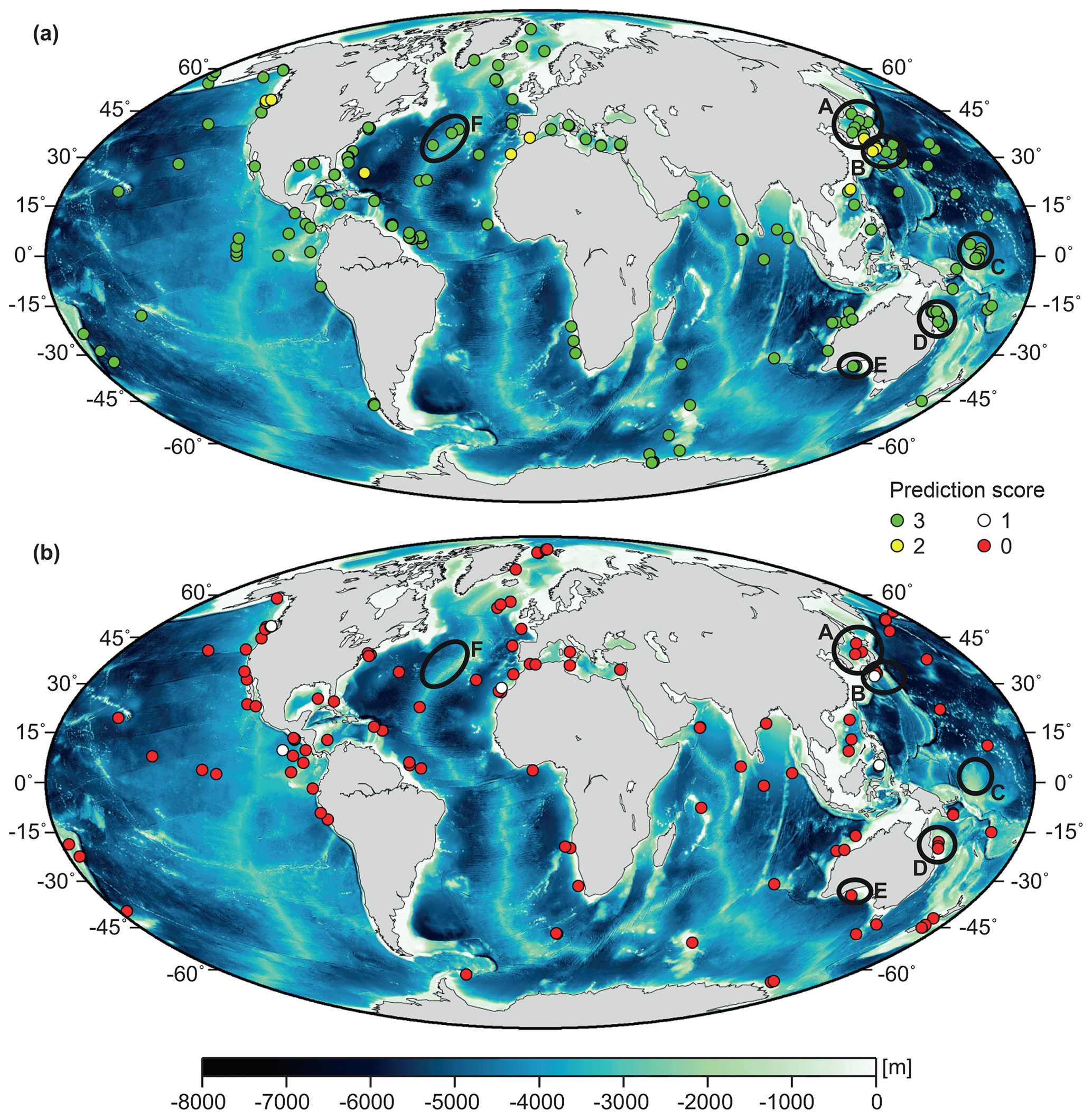
Figure 5Distribution of boreholes with (a) good (scores 2 and 3) and (b) bad (scores 0 and 1) vp predictions. Areas A–E mark clusters of boreholes in the Sea of Japan (A), the Nankai Trough (B), the Ontong Java Plateau (C), the Queensland Plateau (D), and the Great Australian Bight (E). Area F indicates an example for remote boreholes of score 3 on the Mid-Atlantic Ridge. Bathymetry (30 s resolution) is from the GEBCO_2014 grid (http://www.gebco.net).
3.3 Predictor importance
For the 38-predictor CV, the 5 most important predictors were “depth2base”, “crustage”, “depth”, “dist2smt”, and “wdepth” (Fig. 6). Continuous predictors and categorical predictors were clearly separated in the predictor importance plot (Fig. 6), with continuous predictors being of high importance in the RF model, whereas categorical predictors appeared less important. The only exception was the categorical predictor variable “spreading_ridge”, which had a slightly higher importance ranking than the continuous predictors “long” and “dist2transform”. Many of the categorical predictors were of negligible (almost 0) importance (Fig. 6).
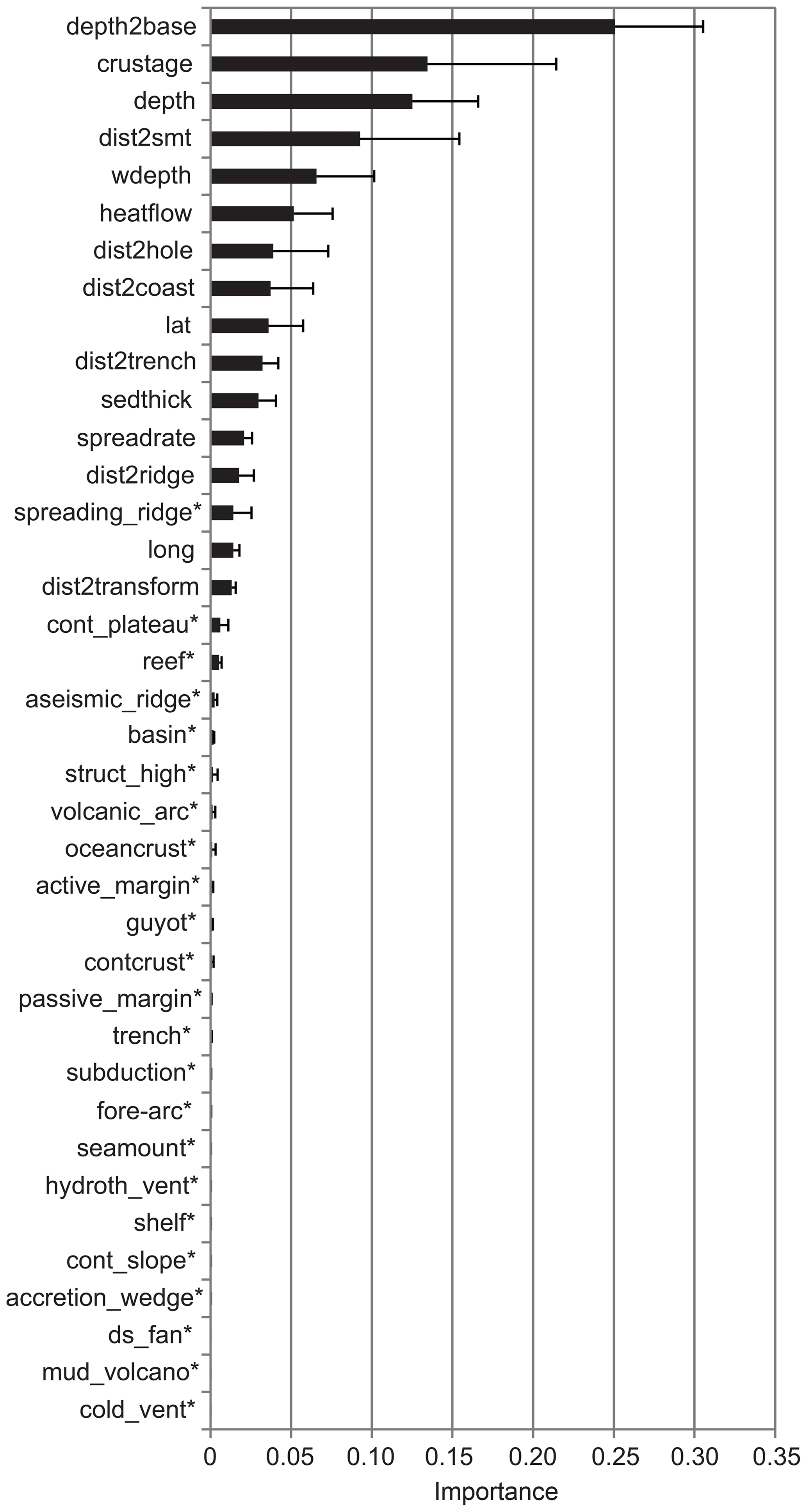
Figure 6Predictor importance ranking for the 38-predictor model run. For each predictor, the importance was averaged over the 10 runs of the 10-fold CV. Categorical predictors are marked with an asterisk. Predictor names are explained in Table 1.
When the least important predictor was eliminated after each model run using RFE, the same trend was observed: in both the unscaled and scaled RFE cases, all categorical predictors were eliminated before the continuous predictors (Table 3). In the 16-predictor case, which had the highest proportion of well-predicted boreholes (61.9 %), the only categorical predictor included was spreading_ridge.
Table 3Predictor ranking based on the RFE results for unscaled and scaled predictors. Categorical predictors are marked with an asterisk. See Table 1 for an explanation of predictor names.
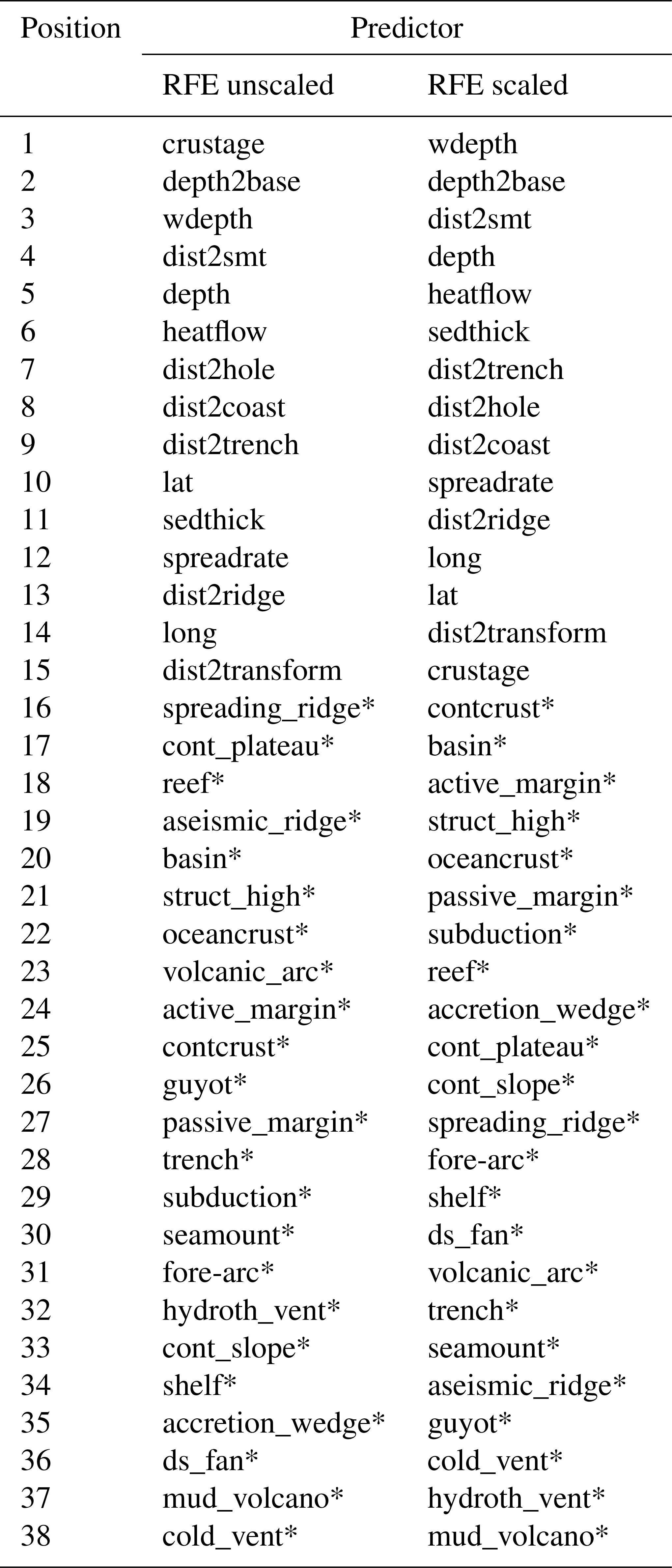
In the unscaled RFE case, the five most important predictors were the same as in the feature importance plot of the 38-predictor case (Fig. 6). However, the order differed slightly, with depth being eliminated before dist2smt, wdepth, depth2base, and crustage (Table 3). When using scaled predictors, the five top predictors included “heatflow” (ranked sixth in both the 38-predictor CV and unscaled RFE cases) instead of crustage. Crustage dropped to position 15 and was thus the least important of the continuous predictors (Table 3). In general, however, the position ranking of most predictors varied only by up to five positions between the unscaled and the scaled RFE cases (Table 3).
4.1 Prediction performance in comparison with empirical functions
Our results show that the general trend of vp(z) profiles can be predicted successfully using machine learning. Overall, the applied RF approach is superior to the empirical vp functions of Hamilton (1985), as indicated by the 60 % of tested boreholes with prediction scores of 3 or 2. Although such a quantitatively better performance (i.e. lower RMSE and MAE and higher R2 than the Hamilton vp(z) profiles) does not always mean a perfect fit to the true vp(z) curve of the tested borehole, the RF approach has a promising potential for the prediction of vp with depth.
Slight improvements of the prediction performance were achieved by applying RFE, resulting in a proportion of well-predicted boreholes of 61.9 % for the 16-predictor model. Smoothing the predicted vp(z) profiles via spline smoothing (spline1 case) provided a further increase to 62.4 % of well-predicted boreholes. In addition, reducing the max_features parameter from 38 (all predictors) to 22 also resulted in a slight improvement (61.3 %), thus supporting other studies that recommended tuning the max_features parameter to improve results (Ließ et al., 2016; Meyer et al., 2018). However, to increase model performance even further, to a proportion of well-predicted boreholes well exceeding 60 %, other changes are required.
4.2 Most important predictors for the prediction of vp(z)
Both the predictor importance ranking of RF and the RFE results revealed depth as one of the most important predictors. However, depth was not the most important predictor, which is surprising as empirical vp functions, including those of Hamilton (1985), all use depth as the only input parameter. Our results showed that depth2base was always ranked higher than depth, and often the predictors wdepth, dist2smt, and crustage also had higher importance scores than depth. Although depth is obviously still an important parameter in the prediction of vp, these observations imply that empirical functions using only depth as input and neglecting all other influences may not produce realistic vp values, which is supported by at least 60 % of test locations for which the RF approach produced better vp(z) profiles than the Hamilton functions.
The high importance of the predictors depth2base, wdepth, dist2smt, crustage, as well as heatflow, seems reasonable. The depth to the basement, which is related to the sediment thickness, is relevant because of the rapid vp increase at the basement contact and the associated transition from relatively low (<2.5 km s−1) to higher (>4 km s−1) vp values. Even though in the majority of boreholes, the basement was not reached, the depth to the basement strongly influences vp. The high ranking of the distance to the nearest seamount is likely attributed to the associated change in heat flow at seamount locations. Higher heat flow and hence higher temperatures affect density, which in turn affects vp. The predictor crustage indicates young oceanic crust, which is characterized by higher temperature and hence lower density, affecting vp. Moreover, crustage differentiates between oceanic (<200 Myr) and continental (here: 1 Gyr) crust and apparently more effectively than the categorical predictors “oceancrust” and contcrust, which are of considerably lower importance.
It has to be noted that the high-importance predictors discussed above only represent the most important of the 38 predictors used for prediction of vp; they are not necessarily the parameters that most strongly influence vp in general. If other parameters, such as porosity, density, pressure, or saturation, had been included as predictors, they would likely have resulted in a higher importance ranking than, e.g. dist2smt or crustage. However, these parameters were not included in the model as they were restricted to measurements at borehole locations – not necessarily those from which vp(z) data were obtained – and are therefore not available for every location in the oceans. For the same reason, other geophysical parameters, e.g. electrical resistivity and magnetic susceptibility, were also not included.
A surprising finding in terms of predictor importance is the low importance of all categorical predictors. The clear separation between continuous and categorical predictors in the predictor importance plots may be due to biased predictor selection, as observed by Strobl et al. (2007) when different types of predictors were used. In such cases, categorical predictors may often be neglected and ignored by the machine learning algorithm (Otey et al., 2006). Scaling the continuous predictors to the same range as the categorical predictors did not help to change the importance ranking, but bias cannot be excluded. The poor representation of some predictors, such as “cold_vent”, “mud_volcano”, and “hydroth_vent” in the dataset, causing these predictors to be 0 for all boreholes in some test folds, likely explains the low importance of these predictors in the predictor ranking, although it is also possible that the geological setting described by the categorical predictors was simply not relevant to the prediction of vp. This possibility appears to be supported by the RFE results, which reveal the best prediction scores (61.9 % well-predicted boreholes) when all but one categorical predictors were excluded (16-predictor case).
4.3 Suggestions for further improvement of performance
The fact that prediction performance could not be much improved by predictor selection, tuning the max_features parameter, or additional smoothing suggests that other measures are needed to further improve the prediction performance. The comparatively high proportion of boreholes with badly predicted vp(z) profiles (about 40 %) is likely due to the limited number of boreholes that were available in this study but may also have been influenced by the choice of machine learning algorithm.
It is possible to add more predictors that potentially influence vp, for example, seafloor gradient, bottom water temperature, and distance to the shelf edge. In addition, some of the predictors could be improved. For example, the age of the continental crust, currently set to the constant value of 1 Gyr, could be adapted based on the crustal age grid by Poupinet and Shapiro (2009). Other studies also suggest including the first and second derivatives of predictors or other mathematical combinations of predictors (Obelcz and Wood, 2018; Wood et al., 2018; Lee et al., 2019).
Another way to extend the dataset is to include more vp(z) data. Given the relatively inhomogeneous global distribution of borehole locations used in this study (Fig. 1), adding more vp(z) data is highly recommended. On a much smaller scale, Gasch et al. (2015) noted that high spatial heterogeneity of input locations limits the prediction performance and increases prediction errors. Adding more vp(z) data, especially from regions such as the southern Pacific and Atlantic oceans that are presently not covered, will likely help to increase the prediction performance. For example, the vp(z) records from recent IODP expeditions may be added to the dataset as they become available. Additional vp data could also be obtained from commercial boreholes and refraction seismic data from ocean bottom seismometers, although the latter would be of lower vertical resolution.
The choice of machine learning algorithm may also influence model performance. Studies comparing RF against other machine learning algorithms reported different trends: in some cases, RF was superior in terms of prediction performance (e.g. Li et al., 2011; Cracknell and Reading, 2014), whereas in other cases, no strong differences were observed between the different methods (e.g. Goetz et al., 2015; Meyer et al., 2016b). However, given the present dataset and its spatial inhomogeneity, we doubt that a different algorithm would lead to a significantly improved prediction performance for vp.
In this study, we presented an RF model for the prediction of vp(z) anywhere in the oceans. In about 60 % of the tested locations, the RF approach produced better vp(z) profiles than empirical vp functions. This indicates a promising potential for the prediction of vp(z) using machine learning, although some improvement is still required. In particular, the model input data should be extended to increase spatial coverage, which is expected to significantly improve prediction performance. Our results showed that depth, which is the only input in empirical vp functions, is not the most important parameter for the prediction of vp. Distance to the basement, water depth, age of crust, and distance to the nearest seamount are, in general, equally or even more important than depth. By including these parameters in the determination of vp, the RF model is able to produce more accurate vp(z) profiles and can therefore be used as an alternative to empirical vp functions. This is of particular interest for geophysical modelling applications, such as modelling gas hydrate concentrations, in areas lacking alternative vp(z) information from boreholes or seismic data.
All vp(z) data used in this study are available through the website of the International Ocean Discovery Program at http://www.iodp.org (last access: 11 November 2019). Additional datasets and grids used are referenced in the Methods section and in Table 1.
ID performed the modelling and analyses, and CB acquired funding for the project. ID prepared the paper with contributions from CB.
The authors declare that they have no conflict of interest.
This study was funded by the Helmholtz Association, grant ExNet-0021. We thank Taylor Lee and an anonymous reviewer for their constructive comments, which helped to improve the paper.
The article processing charges for this open-access publication were covered by a Research Centre of the Helmholtz Association.
This paper was edited by Tarje Nissen-Meyer and reviewed by Taylor Lee and one anonymous referee.
Belgiu, M., Drăguţ, L.: Random forest in remote sensing: A review of applications and future directions, ISPRS J. Photogramm., 114, 24–31, https://doi.org/10.1016/j.isprsjprs.2016.01.011, 2016.
Breiman, L.: Random forests, Mach. Learn., 45, 5–32, https://doi.org/10.1023/A:1010933404324, 2001.
Brune, S., Babeyko, A. Y., Gaedicke, C., and Ladage, S.: Hazard assessment of underwater landslide-generated tsunamis: a case study in the Padang region, Indonesia, Nat. Hazards, 53, 205–218, https://doi.org/10.1007/s11069-009-9424-x, 2010.
Bünz, S., Mienert, J., Vanneste, M., and Andreassen, K.: Gas hydrates at the Storegga Slide: constraints from an analysis of multicomponent, wide-angle seismic data, Geophysics, 70, B19–B34, https://doi.org/10.1190/1.2073887, 2005.
Coffin, M. F., Gahagan, L. M., and Lawver, L. A.: Present-day plate boundary digital data compilation, UTIG Technical Report No. 174, University of Texas Institute for Geophysics, Austin, TX, 1998.
Cracknell, M. J. and Reading, A. M.: Geologial mapping using remote sensing data: A comparison of five machine learning algorithms, their response to variations in the spatial distribution of training data and the use of explicit spatial information, Comput. Geosci., 63, 22–33, https://doi.org/10.1016/j.cageo.2013.10.008, 2014.
Crutchley, G. J., Pecher, I. A., Gorman, A. R., Henrys, S. A., and Greinert, J.: Seismic imaging of gas conduits beneath seafloor seep sites in a shallow marine gas hydrate province, Hikurangi Margin, New Zealand, Mar. Geol., 272, 114–126, https://doi.org/10.1016/j.margeo.2009.03.007, 2010.
Crutchley, G. J., Berndt, C., Klaeschen, D., and Masson, D. G.: Insights into active deformation in the Gulf of Cadiz from new 3-D seismic and high-resolution bathymetry data, Geochem. Geophys. Geosyst., 12, Q07016, https://doi.org/10.1029/2011GC003576, 2011.
Crutchley, G. J., Karstens, J., Berndt, C., Talling, P. J., Watt, S., Vardy, M., Hühnerbach, V., Urlaub, M., Sarkar, S., Klaeschen, D., Paulatto, M., Le Friant, A., Lebas, E., and Maeno, F.: Insights into the emplacement dynamics of volcanic landslides from high-resolution 3D seismic data acquired offshore Montserrat, Lesser Antilles, Mar. Geol., 335, 1–15, https://doi.org/10.1016/j.margeo.2012.10.004, 2013.
Crutchley, G. J., Klaeschen, D., Planert, L., Bialas, J., Berndt, C., Papenberg, C., Hensen, C., Hornbach, M. J., Krastel, S., and Brueckmann, W.: The impact of fluid advection on gas hydrate stability: Investigations at sites of methane seepage offshore Costa Rica, Earth Planet. Sc. Lett., 401, 95–109, https://doi.org/10.1016/j.epsl.2014.05.045, 2014.
Davies, J. H.: Global map of solid Earth surface heat flow, Geochem. Geophys. Geosyst., 14, 4608–4622, https://doi.org/10.1002/ggge.20271, 2013.
Dumke, I., Berndt, C., Crutchley, G. J., Krause, S., Liebetrau, V., Gay, A., and Couillard, M.: Seal bypass at the Giant Gjallar Vent (Norwegian Sea): Indications for a new phase of fluid venting at a 56-Ma-old fluid migration system, Mar. Geol., 351, 38–52, https://doi.org/10.1016/j.margeo.2014.03.006, 2014.
Gasch, C. K., Hengl, T., Gräler, B., Meyer, H., Magney, T., and Brown, D. J.: Spatio-temporal interpolation of soil water, temperature, and electrical conductivity in 3D+T: The Cook Agronomy Farm data set, Spat. Stat., 14, 70–90, https://doi.org/10.1016/j.spasta.2015.04.001, 2015.
Goetz, J. N., Brenning, A., Petschko, H., and Leopold, P.: Evaluating machine learning and statistical prediction techniques for landslide susceptibility modelling, Comput. Geosci., 81, 1–11, https://doi.org/10.1016/j.cageo.2015.04.007, 2015.
Hamilton, E. L.: vp/Vs and Poisson's ratios in marine sediments and rocks, J. Acoust. Soc. Am., 66, 1093–1101, https://doi.org/10.1121/1.383344, 1979.
Hamilton, E. L.: Geoacoustic modeling of the sea floor, J. Acoust. Soc. Am., 68, 1313–1337, https://doi.org/10.1121/1.385100, 1980.
Hamilton, E. L.: Sound velocity as a function of depth in marine sediments, J. Acoust. Soc. Am., 78, 1348–1355, https://doi.org/10.1121/1.392905, 1985.
Karakus, M.: Function identification for the intrinsic strength and elastic properties of granitic rocks via genetic programming (GP), Comput. Geosci., 37, 1318–1323, https://doi.org/10.1016/j.cageo.2010.09.002, 2011.
Kim, S.-S. and Wessel, P.: New global seamount census from altimetry-derived gravity data, Geophys. J. Int., 186, 615–631, https://doi.org/10.1111/j.1365-246X.2011.05076.x, 2011.
Krabbenhoeft, A., Bialas, J., Klaucke, I., Crutchley, G., Papenberg, C., and Netzeband, G. L.: Patterns of subsurface fluid-flow at cold seeps: The Hikurangi Margin, offshore New Zealand, Mar. Pet. Geol., 39, 59–73, https://doi.org/10.1016/j.marpetgeo.2012.09.008, 2013.
Lary, D. J., Alavi, A. H., Gandomi, A. H., and Walker, A. L.: Machine learning in the geosciences and remote sensing. Geosci. Front., 7, 3–10, https://doi.org/10.1016/j.gsf.2015.07.003, 2016.
Lee, T. R., Wood, W. T., and Phrampus, B. J.: A machine learning (kNN) approach to predicting global seafloor total organic carbon, Global Biochem. Cy., 33, 37–46, https://doi.org/10.1029/2018GB005992, 2019.
Li, J., Heap, A. D., Potter, A., and Daniell, J. J.: Application of machine learning methods to spatial interpolation of environmental variables, Environ. Modell. Softw., 26, 1647–1659, https://doi.org/10.1016/j.envsoft.2011.07.004, 2011.
Ließ, M., Schmidt, J., and Glaser, B.: Improving the spatial prediction of soil organic carbon stocks in a complex tropical mountain landscape by methodological specifications in machine learning approaches, PLoS ONE, 11, e0153673, https://doi.org/10.1371/journal.pone.0153673, 2016.
Lilley, F. E. M., Filloux, J. H., Mulhearn, P. J., and Ferguson, I. J.: Magnetic signals from an ocean eddy, J. Geomagn. Geoelectr., 45, 403–422, https://doi.org/10.5636/jgg.45.403, 1993.
Martin, K. M., Wood, W. T., and Becker, J. J.: A global prediction of seafloor sediment porosity using machine learning, Geophys. Res. Lett., 42, 10640–10646, https://doi.org/10.1002/2015GL065279, 2015.
Meyer, H., Katurji, M., Appelhans, T., Müller, M. U., Nauss, T., Roudier, P., and Zawar-Reza, P.: Mapping daily air temperature for Antarctica based on MODIS LST, Remote Sens., 8, 732, https://doi.org/10.3390/rs8090732, 2016a.
Meyer, H., Kühnlein, M., Appelhans, T., and Nauss, T.: Comparison of four machine learning algorithms for their applicability in satellite-based optical rainfall retrievals, Atmos. Res., 169, 424–433, https://doi.org/10.1016/j.atmosres.2015.09.021, 2016b.
Meyer, H., Lehnert, L. W., Wang, Y., Reudenbach, C., Nauss, T., and Bendix, J.: From local spectral measurements to maps of vegetation cover and biomass on the Qinghai-Tibet-Plateau: Do we need hyperspectral information?, Int. J. Appl. Earth Obs. Geoinf., 55, 21–31, https://doi.org/10.1016/j.jag.2016.10.001, 2017.
Meyer, H., Reudenbach, C., Hengl, T., Katurji, M., and Nauss, T.: Improving performance of spatio-temporal machine learning models using forward feature selection and target-oriented validation, Environ. Modell. Softw., 101, 1–9, https://doi.org/10.1016/j.envsoft.2017.12.001, 2018.
Micheletti, N., Foresti, L., Robert, S., Leuenberger, M., Pedrazzini, A., Jaboyedoff, M., and Kanevski, M.: Machine learning feature selection methods for landslide susceptibility mapping, Math. Geosci., 46, 33–57, https://doi.org/10.1007/s11004-013-9511-0, 2014.
Mienert, J., Bünz, S., Guidard, S., Vanneste, M., and Berndt, C.: Ocean bottom seismometer investigations in the Ormen Lange area offshore mid-Norway provide evidence for shallow gas layers in subsurface sediments, Mar. Pet. Geol., 22, 287–297, https://doi.org/10.1016/j.marpetgeo.2004.10.020, 2005.
Müller, A. C. and Guido, S.: Introduction to Machine Learning with Python, O'Reilly Media, Sebastopol, CA, 2017.
Müller, D., Sdrolias, M., Gaina, C., and Roest, W. R.: Age, spreading rates, and spreading asymmetry of the world's ocean crust, Geochem. Geophys. Geosyst., 9, Q04006, https://doi.org/10.1029/2007GC001743, 2008.
Netzeband, G. L., Krabbenhoeft, A., Zillmer, M., Petersen, C. J., Papenberg, C., and Bialas, J.: The structures beneath submarine methane seeps: Seismic evidence from Opouawe Bank, Hikurangi Margin, New Zealand, Mar. Geol., 272, 59–70, https://doi.org/10.1016/j.margeo.2009.07.005, 2010.
Obelcz, J. and Wood, W. T.: Towards a quantitative understanding of parameters driving submarine slope failure: A machine learning approach, EGU General Assembly, Vienna, Austria, 8–13 April 2018, EGU2018-9778, 2018.
Otey, M. E., Ghoting, A., and Parthasarathy, S.: Fast distributed outlier detection in mixed-attribute data sets, Data Min. Knowl. Disc., 12, 203–228, https://doi.org/10.1007/s10618-005-0014-6, 2006.
Pedregosa, F., Varoquaux, G., Gramfort, A., Michel, V., Thirion, B., Grisel, O., Blondel, M., Prettenhofer, P., Weiss, R., Dubourg, V., Vanderplas, J., Passos, A., Cournapeau, D., Brucher, M., Perrot, M., and Duchesnay, E.: Scikit-learn: Machine learning in Python, J. Mach. Learn. Res., 12, 1825–2830, 2011.
Plaza-Faverola, A., Bünz, S., and Mienert, J.: Fluid distributions inferred from P-wave velocity and reflection seismic amplitude anomalies beneath the Nyegga pockmark field of the mid-Norwegian margin, Mar. Pet. Geol., 27, 46–60, https://doi.org/10.1016/j.marpetgeo.2009.07.007, 2010a.
Plaza-Faverola, A., Westbrook, G. K., Ker, S., Exley, R. J. K., Gailler, A., Minshull, T. A., and Broto, K.: Evidence from three-dimensional seismic tomography for a substantial accumulation of gas hydrate in a fluid-escape chimney in the Nyegga pockmark field, offshore Norway, J. Geophys. Res.-Sol. Ea., 115, B08104, https://doi.org/10.1029/2009JB007078, 2010b.
Plaza-Faverola, A., Klaeschen, D., Barnes, P., Pecher, I., Henrys, S., and Mountjoy, J.: Evolution of fluid expulsion and concentrated hydrate zones across the southern Hikurangi subduction margin, New Zealand: An analysis from depth migrated seismic data, Geochem. Geophys. Geosyst., 13, Q08018, https://doi.org/10.1029/2012GC004228, 2012.
Plaza-Faverola, A., Pecher, I., Crutchley, G., Barnes, P. M., Bünz, S., Golding, T., Klaeschen, D., Papenberg, C., and Bialas, J.: Submarine gas seepage in a mixed contractional and shear deformation regime: Cases from the Hikurangi oblique-subduction margin. Geochem. Geophys. Geosyst., 15, 416–433, https://doi.org/10.1002/2013GC005082, 2014.
Poupinet, G. and Shapiro, N. M.: Worldwide distribution of ages of the continental lithosphere derived from a global seismic tomographic model, Lithos, 109, 125–130, https://doi.org/10.1016/j.lithos.2008.10.023, 2009.
Priddy, K. L. and Keller, P. E.: Artificial Neural Networks: an Introduction, SPIE Press, Bellingham, WA, 2005.
Scanlon, G. A., Bourke, R. H., and Wilson, J. H.: Estimation of bottom scattering strength from measured and modeled mid-frequency sonar reverberation levels, IEEE J. Ocean. Eng., 21, 440–451, https://doi.org/10.1109/48.544055, 1996.
Strobl, C., Boulesteix, A.-L., Zeileis, A., and Hothorn, T.: Bias in random forest variable importance measures: Illustrations, sources and a solution, BMC Bioinformatics, 8, 25, https://doi.org/10.1186/1471-2105-8-25, 2007.
Vapnik, V. N. The Nature of Statistical Learning Theory, 2nd edn. Springer, New York, NY, 314 pp., 2000.
Wang, J., Guo, C., Hou, Z., Fu, Y., and Yan, J.: Distributions and vertical variation patterns of sound speed of surface sediments in South China Sea, J. Asian Earth Sci., 89, 46–53, https://doi.org/10.1016/j.jseaes.2014.03.026, 2014.
Wei, C.-L., Rowe, G. T., Escobar-Briones, E., Boetius, A., Soltwedel, T., Caley, M. J., Soliman, Y., Huettmann, F., Qu, F., Yu, Z., Pitcher, C. R., Haedrich, R. L., Wicksten, M. K., Rex, M. A., Baguley, J. G., Sharma, J., Danovaro, R., MacDonald, I. R., Nunnally, C. C., Deming, J. W., Montagna, P., Lévesque, M., Weslawski, J. M., Wlodarska-Kowalczuk, M., Ingole, B. S., Bett, B. J., Billett, D. S. M., Yool, A., Bluhm, B. A., Iken, K., and Narayanaswamy, B. E.: Global patterns and predictions of seafloor biomass using random forests, PLoS ONE, 5, e15323, https://doi.org/10.1371/journal.pone.0015323, 2010.
Wessel, P. and Smith, W. H. F.: A global, self-consistent, hierarchical, high-resolution shoreline database, J. Geophys. Res., 101, 8741–8743, https://doi.org/10.1029/96JB00104, 1996.
Wessel, P., Smith, W. H. F., Scharroo, R., Luis, J., and Wobbe, F.: Generic Mapping Tools: Improved version released, EOS Trans. Am. Geophys. Union, 94, 409–410, https://doi.org/10.1002/2013EO450001, 2013.
Westbrook, G. K., Chand, S., Rossi, G., Long, C., Bünz, S., Camerlenghi, A., Carcione, J. M., Dean, S., Foucher, J.-P., Flueh, E., Gei, D., Haacke, R. R., Madrussani, G., Mienert, J., Minshull, T. A., Nouzé, H., Peacock, S., Reston, T. J., Vanneste, M., and Zillmer, M.: Estimation of gas hydrate concentration from multi-component seismic data at sites on the continental margins of NW Svalbard and the Storegga region of Norway. Mar. Pet. Geol., 25, 744–758, https://doi.org/10.1016/j.marpetgeo.2008.02.003, 2008.
Whittaker, J. M., Goncharov, A., Williams, S., Müller, R. D., and Leitchenkov, G.: Global sediment thickness data set uploaded for the Australian-Antarctic Southern Ocean. Geochem. Geophys. Geosyst., 14, 3297–3305, https://doi.org/10.1002/ggge.20181, 2013.
Wood, W., Lee, T., and Obelcz, J.: Practical quantification of uncertainty in seabed property prediction using geospatial KNN machine learning, EGU General Assembly, Vienna, Austria, 8–13 April 2018, EGU2018-9760, 2018.