Green's theorem in seismic imaging across the scales

The earthquake seismology and seismic exploration communities have developed a variety of seismic imaging methods for passive- and active-source data. Despite the seemingly different approaches and underlying principles, many of those methods are based in some way or another on Green's theorem. The aim of this paper is to discuss a variety of imaging methods in a systematic way, using a specific form of Green's theorem (the homogeneous Green's function representation) as a common starting point. The imaging methods we cover are time-reversal acoustics, seismic interferometry, back propagation, source–receiver redatuming and imaging by double focusing. We review classical approaches and discuss recent developments that fully account for multiple scattering, using the Marchenko method. We briefly indicate new applications for monitoring and forecasting of responses to induced seismic sources, which are discussed in detail in a companion paper.

1 Introduction

Through the years, the earthquake seismology and seismic exploration communities have developed a variety of seismic imaging methods for passive- and active-source data, based on a wide range of principles such as time-reversal acoustics, Green's function retrieval by noise correlation (a form of seismic interferometry), back propagation (also known as holography) and source–receiver redatuming. Many of these methods are rooted in some way or another in Green's theorem (Green, 1828; Morse and Feshbach, 1953; Challis and Sheard, 2003). The current paper is a modest attempt to discuss a variety of imaging methods and their underlying principles in a systematic way, using Green's theorem as the common starting point. We are certainly not the first to recognize links between different imaging methods. For example, Esmersoy and Oristaglio (1988) discussed the link between back propagation and reverse-time migration, Derode et al. (2003) derived Green's function retrieval from the principle of time-reversal acoustics by physical reasoning and Schuster et al. (2004) linked seismic interferometry to back propagation, to name but a few.

We start by reviewing a specific form of Green's theorem, namely the classical representation of the homogeneous Green's function, originally developed for optical holography (Porter, 1970; Porter and Devaney, 1982). The homogeneous Green's function is the superposition of the causal Green's function and its time reversal. We use its surface-integral representation to derive time-reversal acoustics, seismic interferometry, back propagation, source–receiver redatuming and imaging by double focusing in a systematic way, confirming that these methods are all very similar. We briefly discuss the potential and the limitations of these methods. Because the classical homogeneous Green's function representation is based on a closed surface integral, an implicit assumption of all of these methods is that the medium of interest can be accessed from all sides. Due to the fact that acquisition is limited to the Earth's surface in most seismic applications, a major part of the closed surface integral is necessarily neglected. This implies that errors are introduced and, in particular, that multiple reflections between layer interfaces are not correctly handled. To address this issue, we also discuss a recently developed single-sided representation of the homogeneous Green's function. We use this to derive, in the same systematic way, modified seismic imaging methods that account for multiple reflections between layer interfaces. In a companion paper (Brackenhoff et al., 2019) we extensively discuss applications for monitoring induced seismicity.

Although the solid Earth supports elastodynamic (vectorial) waves, to facilitate the comparison of the different methods discussed in this paper we have chosen to consider scalar waves only. Scalar waves, which obey the acoustic wave equation, serve as an approximation for compressional body waves propagating through the solid Earth, or for the fundamental mode of surface waves propagating along the Earth's surface, depending on the application. In several places we give references to extensions of the methods that account for the full elastodynamic wave field.

2 Theory and applications of a classical wave field representation

2.1 Classical homogeneous Green's function representation

We consider an inhomogeneous lossless acoustic medium, with mass density ρ(x) and compressibility κ(x), where $\mathit{x}=(x_{\mathrm{1}},x_{\mathrm{2}},x_{\mathrm{3}})$ denotes the Cartesian coordinate vector. In this medium we define a unit impulsive point source of volume-injection rate density $q(\mathit{x},t)=\mathit{\delta }(\mathit{x}-{\mathit{x}}_{\mathrm{A}})\mathit{\delta }\left(t\right)$, where δ(⋅) denotes the Dirac delta function, x_A represents the position of the source and t stands for time. The response to this source, observed at any position x in the inhomogeneous medium, is the Green's function $G(\mathit{x},{\mathit{x}}_{\mathrm{A}},t)$ and obeys the following wave equation:

$$\begin{array}{}\text{(1)}& {\partial }_i\left({\mathit{\rho }}^{-\mathrm{1}}{\partial }_{i}G\right)-\mathit{\kappa }{\partial }_t^{\mathrm{2}}G=-\mathit{\delta }(\mathit{x}-{\mathit{x}}_{\mathrm{A}}){\partial }_t\mathit{\delta }\left(t\right),\end{array}$$

where ∂_t stands for the temporal differential operator $\partial /\partial t$ and ∂_i represents the spatial differential operator $\partial /\partial x_i$. Latin subscripts (except t) take on the values 1, 2 and 3, and Einstein's summation convention applies to repeated subscripts. We impose the condition $G(\mathit{x},{\mathit{x}}_{\mathrm{A}},t)=\mathrm{0}$ for t<0, so that $G(\mathit{x},{\mathit{x}}_{\mathrm{A}},t)$ for t>0 is the causal solution of Eq. (1), representing a wave field originating from the source at x_A. Note that the Green's function obeys source–receiver reciprocity, i.e., $G({\mathit{x}}_{\mathrm{B}},{\mathit{x}}_{\mathrm{A}},t)=G({\mathit{x}}_{\mathrm{A}},{\mathit{x}}_{\mathrm{B}},t)$, assuming both are causal and obey the same boundary conditions (Rayleigh, 1878; Landau and Lifshitz, 1959; Morse and Ingard, 1968). This property will be frequently used without always mentioning it explicitly.

The time-reversal of the Green's function, $G(\mathit{x},{\mathit{x}}_{\mathrm{A}},-t)$, is the acausal solution of Eq. (1), which, for t<0, represents a wave field converging to a sink at x_A. The homogeneous Green's function $G_{\mathrm{h}}(\mathit{x},{\mathit{x}}_{\mathrm{A}},t)$ is defined as the superposition of the Green's function and its time reversal, according to

$$\begin{array}{}\text{(2)}& G_{\mathrm{h}}(\mathit{x},{\mathit{x}}_{\mathrm{A}},t)=G(\mathit{x},{\mathit{x}}_{\mathrm{A}},t)+G(\mathit{x},{\mathit{x}}_{\mathrm{A}},-t).\end{array}$$

It is called “homogeneous” because it obeys a homogeneous wave equation, i.e., a wave equation without a singularity on the right-hand side. Hence ${\partial }_i\left({\mathit{\rho }}^{-\mathrm{1}}{\partial }_i{G}_{\mathrm{h}}\right)-\mathit{\kappa }{\partial }_t^{\mathrm{2}}{G}_{\mathrm{h}}=\mathrm{0}$, in which the medium parameters ρ(x) and κ(x) are generally not homogeneous. Note that in this paper we use the adjective “homogeneous” in two different ways. We define the Fourier transform of a time-dependent function u(t) as

$$\begin{array}{}\text{(3)}& u\left(\mathit{\omega }\right)=\underset{-\mathrm{\infty }}{\overset{\mathrm{\infty }}{\int }}u\left(t\right)\exp \left(i\mathit{\omega }t\right)\mathrm{d}t.\end{array}$$

Here ω denotes angular frequency and i the imaginary unit. For notational convenience, we use the same symbol for quantities in the time domain and in the frequency domain. The wave equation for the Green's function in the frequency domain reads

$$\begin{array}{}\text{(4)}& {\partial }_i\left({\mathit{\rho }}^{-\mathrm{1}}{\partial }_{i}G\right)+\mathit{\kappa }{\mathit{\omega }}^{\mathrm{2}}G=i\mathit{\omega }\mathit{\delta }(\mathit{x}-{\mathit{x}}_{\mathrm{A}}).\end{array}$$

The homogeneous Green's function in the frequency domain is defined as

$$\begin{array}{ll}{\displaystyle }{G}_{\mathrm{h}}(\mathit{x},{\mathit{x}}_{\mathrm{A}},\mathit{\omega })& {\displaystyle }=G(\mathit{x},{\mathit{x}}_{\mathrm{A}},\mathit{\omega })+G^{*}(\mathit{x},{\mathit{x}}_{\mathrm{A}},\mathit{\omega })\\ \text{(5)}& {\displaystyle }& {\displaystyle }=\mathrm{2}\mathrm{\Re }\mathit{\left\{}G\right(\mathit{x},{\mathit{x}}_{\mathrm{A}},\mathit{\omega }\left)\mathit{\right\}},\end{array}$$

where the superscript asterisk denotes complex conjugation, and ℜ means that the real part is taken. The classical representation of the homogeneous Green's function reads (Porter, 1970; Oristaglio, 1989; Supplement, Sect. S1.3)

$$\begin{array}{ll}{\displaystyle }{G}_{\mathrm{h}}({\mathit{x}}_{\mathrm{B}},{\mathit{x}}_{\mathrm{A}},\mathit{\omega })& {\displaystyle }=\underset{\mathbb{S}}{\oint }{\displaystyle \frac{\mathrm{1}}{i\mathit{\omega }\mathit{\rho }\left(\mathit{x}\right)}}\left(\mathit{\right\{}{\partial }_{i}G(\mathit{x},{\mathit{x}}_{\mathrm{B}},\mathit{\omega })\mathit{\left\}}{G}^{*}\right(\mathit{x},{\mathit{x}}_{\mathrm{A}},\mathit{\omega })\\ \text{(6)}& {\displaystyle }& {\displaystyle }-G(\mathit{x},{\mathit{x}}_{\mathrm{B}},\mathit{\omega }){\partial }_i{G}^{*}(\mathit{x},{\mathit{x}}_{\mathrm{A}},\mathit{\omega }))n_i\mathrm{d}\mathit{x},\end{array}$$

see Fig. 1. Here 𝕊 is an arbitrarily shaped closed surface with an outward pointing normal vector $\mathit{n}=(n_{\mathrm{1}},n_{\mathrm{2}},n_{\mathrm{3}})$, which does not necessarily coincide with the boundary of the medium. It is assumed that x_A and x_B are situated inside 𝕊. Note that the aforementioned authors use a slightly different definition of the Green's function (the factor iω in the source term in Eq. (4) is absent in their case). Nevertheless, we will refer to Eq. (6) as the classical homogeneous Green's function representation. When 𝕊 is sufficiently smooth and the medium outside 𝕊 is homogeneous (with mass density ρ₀, compressibility κ₀ and propagation velocity $c_{\mathrm{0}}=({\mathit{\kappa }}_{\mathrm{0}}{\mathit{\rho }}_{\mathrm{0}}{)}^{-\mathrm{1}/\mathrm{2}}$), the two terms under the integral in Eq. (6) are nearly identical (but opposite in sign); hence, this representation may be approximated by

$$\begin{array}{}\text{(7)}& G_{\mathrm{h}}({\mathit{x}}_{\mathrm{B}},{\mathit{x}}_{\mathrm{A}},\mathit{\omega })=-\mathrm{2}\underset{\mathbb{S}}{\oint }{\displaystyle \frac{\mathrm{1}}{i\mathit{\omega }{\mathit{\rho }}_{\mathrm{0}}}}G(\mathit{x},{\mathit{x}}_{\mathrm{B}},\mathit{\omega }){\partial }_i{G}^{*}(\mathit{x},{\mathit{x}}_{\mathrm{A}},\mathit{\omega })n_i\mathrm{d}\mathit{x}.\end{array}$$

The main approximation is that evanescent waves are neglected (Zheng et al., 2011; Wapenaar et al., 2011).

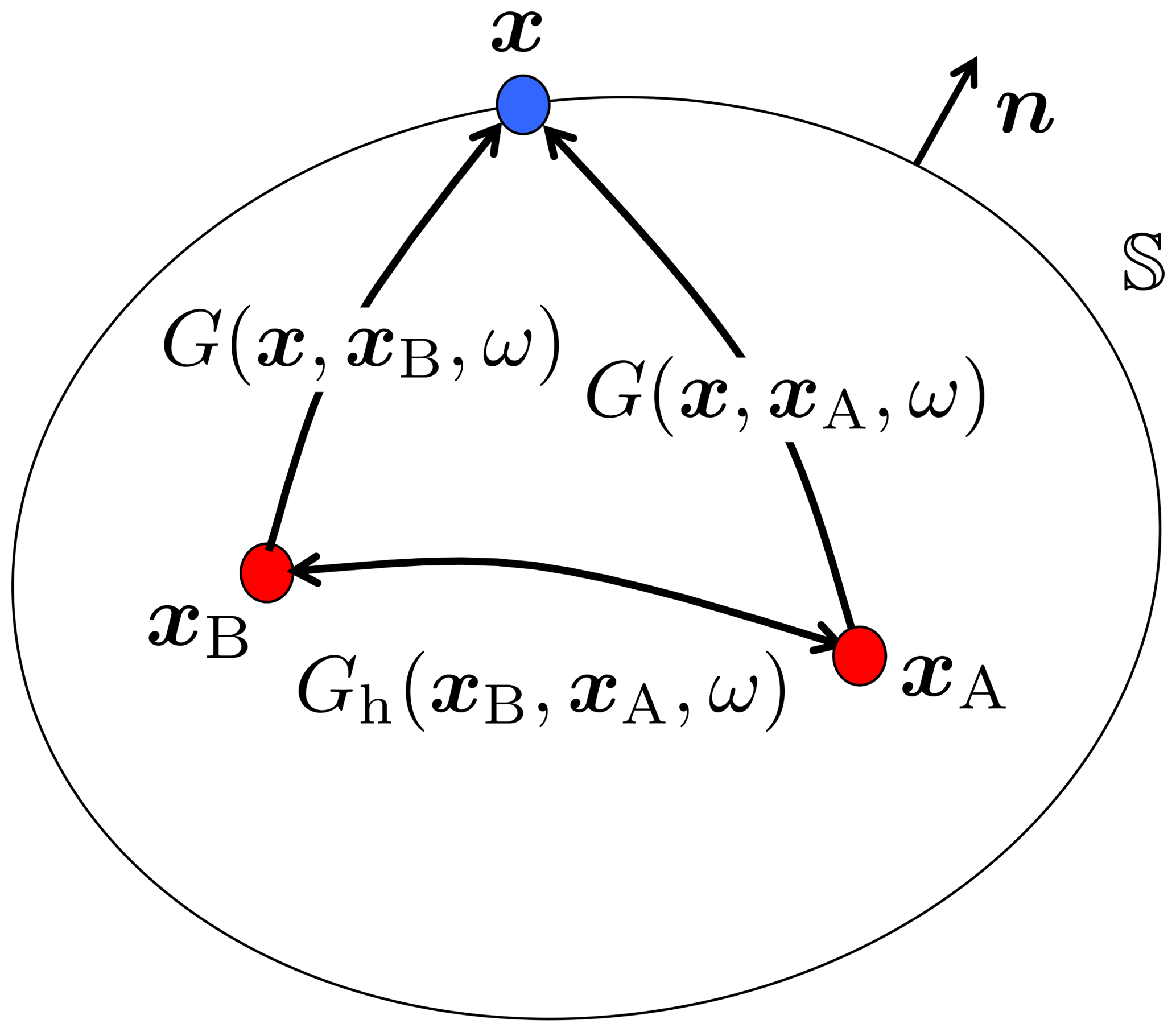
Figure 1 Configuration for the homogeneous Green's function representation (Eq. 6). The rays in this and subsequent figures represent the full responses between the source and receiver points, including primary and multiple scattering.

In the following sections we discuss different imaging methods. Each time we first introduce the specific method in an intuitive way, after which we present a more quantitative derivation based on Eq. (7).

2.2 Time-reversal acoustics

Time-reversal acoustics has been pioneered by Fink and co-workers (Fink, 1992, 2006; Derode et al., 1995; Draeger and Fink, 1999). It makes use of the fact that the acoustic wave equation for a lossless medium is invariant under time reversal (for discussions regarding elastodynamic time-reversal methods we refer the reader to Scalerandi et al., 2009; Anderson et al., 2009; Wang and McMechan, 2015). Hence, given a particular solution of the wave equation, its time-reversal obeys the same wave equation. Figure 2 illustrates the principle (following Derode et al., 1995, and Fink, 2006). In Fig. 2a, an impulsive source at x_A emits a wave field which, after propagation through a highly scattering medium, is recorded by receivers at x on the surface 𝕊₀. In the practice of time-reversal acoustics, 𝕊₀ is a finite open surface. We discuss the limitations of this later. The recordings at 𝕊₀ are denoted as $v_{\mathrm{n}}(\mathit{x},{\mathit{x}}_{\mathrm{A}},t)$, where v_n stands for the normal component of the particle velocity. Note that these recordings are very complex due to multiple scattering in the medium. In Fig. 2b, the time-reversals of these complex recordings, $v_{\mathrm{n}}(\mathit{x},{\mathit{x}}_{\mathrm{A}},-t)$, are emitted from the surface 𝕊₀ into the medium. After propagating through the same scattering medium, the field should focus at x_A, i.e., at the position of the original source. Figure 2c shows a snapshot of the field at t=0, which indeed contains a focus at x_A. Figure 2d shows a horizontal cross-section of the amplitudes at t=0 at the depth level of the focus (the solid blue curve with the sharp peak). For comparison, the dotted red curve shows the amplitude cross-section of the focus that is obtained with a similar time-reversal experiment in absence of scatterers. As the solid blue curve has a sharper peak than the dotted red curve, we can conclude that multiple scattering contributes to the formation of the focus in Fig. 2c. The scattering medium effectively widens the aperture angle, which explains the better focus.

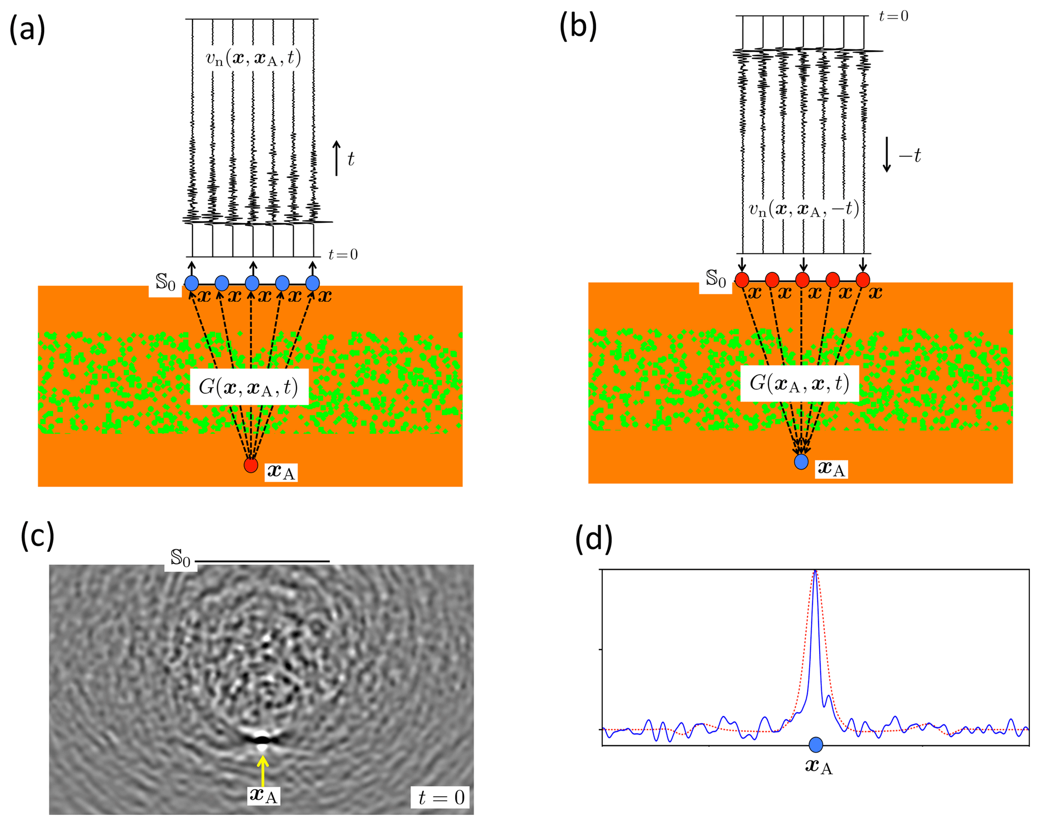
Figure 2 Principle of time-reversal acoustics. (a) Forward propagation from x_A to the finite open surface 𝕊₀. (b) Emission of the time-reversed recordings from 𝕊₀ into the medium. (c) Snapshot of the wave field at t=0, with focus at x_A. (d) Solid blue curve: amplitude cross-section of the focused field in (c), taken along a horizontal line through the focal point x_A. Dotted red curve: amplitude cross-section obtained from a similar time-reversal experiment, in the absence of scatterers.

The time-reversal principle can be made more quantitative using Green's theorem (Fink, 2006). First, using the equation of motion, we express the normal component of the particle velocity at 𝕊 in the frequency domain as

$$\begin{array}{}\text{(8)}& v_{\mathrm{n}}(\mathit{x},{\mathit{x}}_{\mathrm{A}},\mathit{\omega })={\displaystyle \frac{\mathrm{1}}{i\mathit{\omega }{\mathit{\rho }}_{\mathrm{0}}}}{\partial }_{i}G(\mathit{x},{\mathit{x}}_{\mathrm{A}},\mathit{\omega })n_{i}s\left(\mathit{\omega }\right),\end{array}$$

where s(ω) is the spectrum of the source at x_A. Using this in the homogeneous Green's function representation of Eq. (7) we obtain

$$\begin{array}{}\text{(9)}& G_{\mathrm{h}}({\mathit{x}}_{\mathrm{B}},{\mathit{x}}_{\mathrm{A}},\mathit{\omega })s^{*}\left(\mathit{\omega }\right)=\mathrm{2}\underset{\mathbb{S}}{\oint }G({\mathit{x}}_{\mathrm{B}},\mathit{x},\mathit{\omega })v_{\mathrm{n}}^{*}(\mathit{x},{\mathit{x}}_{\mathrm{A}},\mathit{\omega })\mathrm{d}\mathit{x},\end{array}$$

or, in the time domain (using Eq. 2),

$$\begin{array}{ll}{\displaystyle }\mathit{\left\{}G\right({\mathit{x}}_{\mathrm{B}},{\mathit{x}}_{\mathrm{A}},t)& {\displaystyle }+G({\mathit{x}}_{\mathrm{B}},{\mathit{x}}_{\mathrm{A}},-t)\mathit{\}}*s(-t)\\ \text{(10)}& {\displaystyle }& {\displaystyle }=\mathrm{2}\underset{\mathbb{S}}{\oint }\underset{\text{“propagator”}}{\underbrace{G({\mathit{x}}_{\mathrm{B}},\mathit{x},t)}}*\underset{\text{“secondary\hspace{0.17em}sources”}}{\underbrace{v_{\mathrm{n}}(\mathit{x},{\mathit{x}}_{\mathrm{A}},-t)}}\mathrm{d}\mathit{x},\end{array}$$

where the inline asterisk (*) denotes temporal convolution. This is the fundamental expression for time-reversal acoustics. The integrand on the right-hand side formulates the propagation of the time-reversed field $v_{\mathrm{n}}(\mathit{x},{\mathit{x}}_{\mathrm{A}},-t)$ through the inhomogeneous medium by the Green's function $G({\mathit{x}}_{\mathrm{B}},\mathit{x},t)$ from the sources at x on the boundary 𝕊 to any receiver position x_B inside the medium. The integral is taken along all source positions x on the closed boundary 𝕊. The right-hand side resembles Huygens' principle, which states that each point of an incident wave field acts as a secondary source, except that here the secondary sources on 𝕊 consist of time-reversed measurements instead of an incident wave field. The left-hand side quantifies the field at any point x_B inside 𝕊, which consists within the negative time of a backward propagating field $G({\mathit{x}}_{\mathrm{B}},{\mathit{x}}_{\mathrm{A}},-t)*s(-t)$, converging to x_A, and within the positive time of a forward propagating field $G({\mathit{x}}_{\mathrm{B}},{\mathit{x}}_{\mathrm{A}},t)*s(-t)$, originating from a virtual source at x_A. By setting x_B equal to x_A we obtain the field at the focus (i.e., at the position of the original source). By taking x_B variable in a small region around x_A, while setting t equal to zero, Eq. (10) quantifies the focal spot. Assuming the source function s(t) is symmetric, this yields

$$\begin{array}{}\text{(11)}& \left[\mathit{\right\{}G({\mathit{x}}_{\mathrm{B}},{\mathit{x}}_{\mathrm{A}},t)+G({\mathit{x}}_{\mathrm{B}},{\mathit{x}}_{\mathrm{A}},-t)\mathit{\}}*s(t){]}_{t=\mathrm{0}}=-{\displaystyle \frac{\overline{\mathit{\rho }}}{\mathrm{2}\mathit{\pi }r}}\dot{s}(d/\overline{c})\end{array}$$

(Douma and Snieder, 2015; Wapenaar and Thorbecke, 2017), where $\overline{c}$ and $\overline{\mathit{\rho }}$ are the propagation velocity and mass density in the neighborhood of x_A, d is the distance of x_B to x_A, and $\dot{s}\left(t\right)$ denotes the derivative of the source function s(t).

It should be noted that the integration in Eq. (10) takes place over sources on a closed surface 𝕊. However, in the example in Fig. 2 the time-reversed field is emitted into the medium from a finite open surface 𝕊₀. Despite this discrepancy, a good focus is obtained around x_A. Nevertheless, Fig. 2c also shows a noisy field at t=0, particularly in the scattering region. According to Eq. (10), this noisy field would vanish if the time-reversed field was emitted from a closed surface into the medium.

Figure 2 is representative of ultrasonic applications of time-reversal acoustics, because in those applications it is feasible to physically emit the time-reversed field into the real medium (Fink, 1992, 2006; Cassereau and Fink, 1992; Derode et al., 1995; Draeger and Fink, 1999; Tanter and Fink, 2014). Time-reversal acoustics also finds applications in geophysics at various scales, but in those applications the time-reversed field is emitted numerically into a model of the Earth. This is used for source characterization (McMechan, 1982; Gajewski and Tessmer, 2005; Larmat et al., 2010) and for structural imaging by reverse-time migration (McMechan, 1983; Whitmore, 1983; Baysal et al., 1983; Etgen et al., 2009; Zhang and Sun, 2009; Clapp et al., 2010). In these model-driven applications it is much more difficult to account for multiple scattering, which is therefore usually ignored. Moreover, the scattering mechanism is often very different, particularly in applications dedicated to imaging the Earth's crust. We discuss a second time-reversal example to illustrate this.

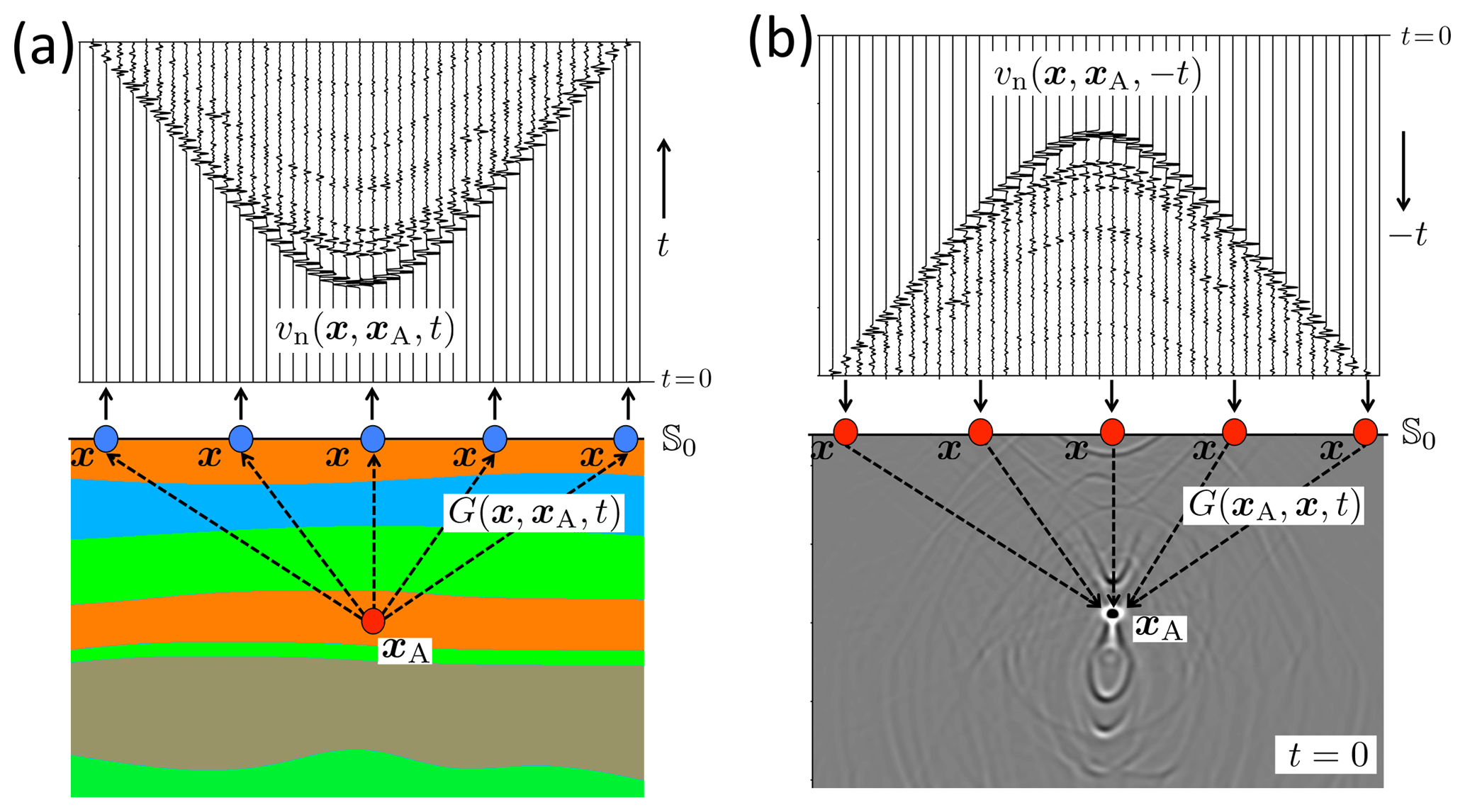
Figure 3 Time-reversal acoustics in a layered medium. (a) Forward propagation from x_A to the finite open surface 𝕊₀. (b) Emission of the time-reversed recordings from 𝕊₀ into the medium and a snapshot of the wave field at t=0, with focus at x_A.

Whereas in Fig. 2 we considered short-period multiple scattering at randomly distributed point-like scatterers in a homogeneous background medium, in Fig. 3 we consider long-period multiple scattering at extended interfaces between layers with distinct medium parameters (which is representative for multiple scattering in the Earth's crust). Figure 3a shows the response $v_{\mathrm{n}}(\mathit{x},{\mathit{x}}_{\mathrm{A}},t)$ to a source at x_A inside a layered medium, observed at the surface 𝕊₀. The time-reversal of this response is emitted from 𝕊₀ into the same layered medium. The field at t=0 is shown in Fig. 3b. We again observe a clear focus at x_A, but this time the multiple scattering does not contribute to the resolution of the focus (because there are no point scatterers that effectively widen the aperture angle). On the contrary, the multiply scattered waves give rise to strong, distinct artefacts in other regions in the medium. Again, these artefacts would disappear entirely if the time-reversed field was emitted from a closed surface, but this is of course unrealistic for geophysical applications. In Sect. 3.2 we discuss a modified approach to single-sided time-reversal acoustics which does not suffer from artefacts such as those in Fig. 3b.

2.3 Seismic interferometry

Under certain conditions, the cross-correlation of passive ambient-noise recordings at two receivers converges to the response that would be measured at one of the receivers if there were an impulsive source at the position of the other. This methodology, which creates a virtual source at the position of an actual receiver, is known as Green's function retrieval by noise correlation (a form of seismic interferometry). At the ultrasonic scale it has been pioneered by Weaver and co-workers (Weaver and Lobkis, 2001, 2002; Lobkis and Weaver, 2001), and the object of investigation at this scale is often a closed system (i.e., a finite specimen with reflecting boundaries on all sides). Early applications for open systems are discussed by Aki (1957), Claerbout (1968), Duvall et al. (1993), Rickett and Claerbout (1999), Schuster (2001), Wapenaar et al. (2002), Campillo and Paul (2003), Derode et al. (2003), Snieder (2004), Schuster et al. (2004), Roux et al. (2005), Sabra et al. (2005a), Larose et al. (2006) and Draganov et al. (2007). A detailed discussion of the many aspects of seismic interferometry is beyond the scope of this paper. Overviews of seismic interferometry, for passive as well as controlled-source data, are given by Schuster (2009), Wapenaar et al. (2010) and Nakata et al. (2019).

Figure 4 illustrates the principle for passive ambient-noise data. In Fig. 4a, a distribution of uncorrelated noise sources N(x,t) at some finite open surface 𝕊₀ emits waves through an inhomogeneous medium to receivers at x_A and x_B. The cross-correlation of the responses at x_A and x_B converges to $G({\mathit{x}}_{\mathrm{B}},{\mathit{x}}_{\mathrm{A}},t)*C_N\left(t\right)$, where C_N(t) is the autocorrelation of the noise. The result is shown in Fig. 4b, for a fixed virtual source at x_A and an array of receivers at variable x_B.

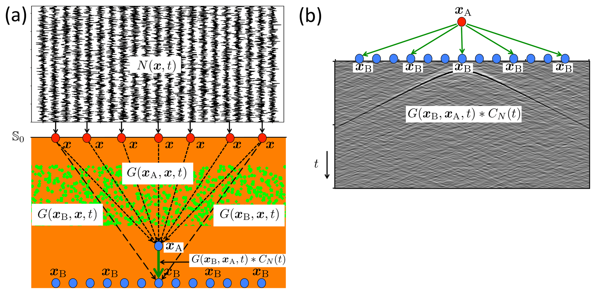
Figure 4 Principle of seismic interferometry. (a) Propagation of ambient noise from 𝕊₀ through an inhomogeneous medium to receivers at x_A and x_B. (b) Cross-correlation of responses at x_A and x_B (with x_A fixed and x_B variable).

We use the homogeneous Green's function representation of Eq. (7) to explain this in a more quantitative way (Wapenaar et al., 2002; Weaver and Lobkis, 2004; van Manen et al., 2005; Korneev and Bakulin, 2006). Representations for elastodynamic interferometry are discussed by Wapenaar (2004), Halliday and Curtis (2008) and Kimman and Trampert (2010). Applying source–receiver reciprocity to the Green's functions under the integral in Eq. (7), we obtain

$$\begin{array}{}\text{(12)}& G_{\mathrm{h}}({\mathit{x}}_{\mathrm{B}},{\mathit{x}}_{\mathrm{A}},\mathit{\omega })=-{\displaystyle \frac{\mathrm{2}}{i\mathit{\omega }{\mathit{\rho }}_{\mathrm{0}}}}\underset{\mathbb{S}}{\oint }G({\mathit{x}}_{\mathrm{B}},\mathit{x},\mathit{\omega }){\partial }_i{G}^{*}({\mathit{x}}_{\mathrm{A}},\mathit{x},\mathit{\omega })n_i\mathrm{d}\mathit{x}.\end{array}$$

The integrand can be interpreted as the Fourier transform of the cross-correlation of responses to sources at x on closed surface 𝕊, observed by receivers at x_A and x_B. Note that 𝕊 is the surface containing the sources; it is not the boundary of the medium. $G({\mathit{x}}_{\mathrm{B}},\mathit{x},\mathit{\omega })$ is the response to a monopole source at x, and ${\partial }_{i}G({\mathit{x}}_{\mathrm{A}},\mathit{x},\mathit{\omega })n_i$ is the response to a dipole source at the same position. In most situations there will only be one type of source present at x; therefore, we approximate the dipole sources by monopole sources, using the far-field approximation:

$$\begin{array}{}\text{(13)}& {\partial }_{i}G({\mathit{x}}_{\mathrm{A}},\mathit{x},\mathit{\omega })n_i\to {\displaystyle \frac{i\mathit{\omega }\left|\cos \right(\mathit{\alpha }\left(\mathit{x}\right)\left)\right|}{c_{\mathrm{0}}}}G({\mathit{x}}_{\mathrm{A}},\mathit{x},\mathit{\omega }).\end{array}$$

Here α(x) is the angle between the normal to 𝕊 at x and the ray from the source at x to the receiver at x_A. When the medium inside 𝕊 is inhomogeneous, there will be multiple rays between x and x_A; hence, the angle α(x) is not unique. Moreover, for passive interferometry the positions of the sources are usually unknown. For simplicity we ignore the $\left|\cos \right(\mathit{\alpha }\left(\mathit{x}\right)\left)\right|$ term in Eq. (13) and substitute the remaining expression into Eq. (12). This yields

$$\begin{array}{}\text{(14)}& G_{\mathrm{h}}({\mathit{x}}_{\mathrm{B}},{\mathit{x}}_{\mathrm{A}},\mathit{\omega })\approx {\displaystyle \frac{\mathrm{2}}{{\mathit{\rho }}_{\mathrm{0}}{c}_{\mathrm{0}}}}\underset{\mathbb{S}}{\oint }G({\mathit{x}}_{\mathrm{B}},\mathit{x},\mathit{\omega })G^{*}({\mathit{x}}_{\mathrm{A}},\mathit{x},\mathit{\omega })\mathrm{d}\mathit{x},\end{array}$$

or, in the time domain (using Eq. 2),

$$\begin{array}{ll}{\displaystyle }G({\mathit{x}}_{\mathrm{B}},{\mathit{x}}_{\mathrm{A}},t)& {\displaystyle }+G({\mathit{x}}_{\mathrm{B}},{\mathit{x}}_{\mathrm{A}},-t)\\ \text{(15)}& {\displaystyle }& {\displaystyle }\approx {\displaystyle \frac{\mathrm{2}}{{\mathit{\rho }}_{\mathrm{0}}{c}_{\mathrm{0}}}}\underset{\mathbb{S}}{\oint }G({\mathit{x}}_{\mathrm{B}},\mathit{x},t)*G({\mathit{x}}_{\mathrm{A}},\mathit{x},-t)\mathrm{d}\mathit{x}\end{array}$$

(the approximation sign refers to the far-field approximation, with the term $\left|\cos \right(\mathit{\alpha }\left(\mathit{x}\right)\left)\right|$ ignored). This expression shows that the Green's function and its time-reversal between x_A and x_B can be approximately retrieved from the cross-correlation of responses to impulsive monopole sources at x on 𝕊, followed by an integration along 𝕊. This expression, and variants of it, are used in situations where responses to individual transient sources are available (Kumar and Bostock, 2006; Schuster and Zhou, 2006; Bakulin and Calvert, 2006; Abe et al., 2007; Tonegawa et al., 2009; Ruigrok et al., 2010). Next, we modify this expression for simultaneous noise sources. For a distribution of noise sources N(x,t) on 𝕊 (like in Fig. 4a), we can write the following for the observed fields at x_A and x_B:

$$\begin{array}{}\text{(16)}& {\displaystyle }& {\displaystyle }p({\mathit{x}}_{\mathrm{A}},t)=\underset{\mathbb{S}}{\oint }G({\mathit{x}}_{\mathrm{A}},\mathit{x},t)*N(\mathit{x},t)\mathrm{d}\mathit{x},\text{(17)}& {\displaystyle }& {\displaystyle }p({\mathit{x}}_{\mathrm{B}},t)=\underset{\mathbb{S}}{\oint }G({\mathit{x}}_{\mathrm{B}},{\mathit{x}}^{\prime },t)*N({\mathit{x}}^{\prime },t)\mathrm{d}{\mathit{x}}^{\prime }.\end{array}$$

Assuming the noise sources are mutually uncorrelated, they obey

$$\begin{array}{}\text{(18)}& \langle N({\mathit{x}}^{\prime },t)*N(\mathit{x},-t)\rangle ={\mathit{\delta }}_{\mathbb{S}}(\mathit{x}-{\mathit{x}}^{\prime })C_N\left(t\right),\end{array}$$

where C_N(t) is the autocorrelation of the noise (which is assumed to be the same for all sources), 〈⋅〉 stands for time averaging and ${\mathit{\delta }}_{\mathbb{S}}(\mathit{x}-{\mathit{x}}^{\prime })$ is a 2-D delta function defined in 𝕊. Cross-correlation of the observed noise fields in x_A and x_B gives

$$\begin{array}{ll}{\displaystyle }\langle p({\mathit{x}}_{\mathrm{B}},t)*p({\mathit{x}}_{\mathrm{A}},-t)\rangle & {\displaystyle }=\langle \underset{\mathbb{S}}{\oint }\underset{\mathbb{S}}{\oint }G({\mathit{x}}_{\mathrm{B}},{\mathit{x}}^{\prime },t)*N({\mathit{x}}^{\prime },t)\\ \text{(19)}& {\displaystyle }& {\displaystyle }*G({\mathit{x}}_{\mathrm{A}},\mathit{x},-t)*N(\mathit{x},-t)\mathrm{d}{\mathit{x}}^{\prime }\mathrm{d}\mathit{x}\rangle .\end{array}$$

Using Eq. (18) this becomes

$$\begin{array}{ll}{\displaystyle }& {\displaystyle }\langle p({\mathit{x}}_{\mathrm{B}},t)*p({\mathit{x}}_{\mathrm{A}},-t)\rangle \\ \text{(20)}& {\displaystyle }& {\displaystyle }=\underset{\mathbb{S}}{\oint }G({\mathit{x}}_{\mathrm{B}},\mathit{x},t)*G({\mathit{x}}_{\mathrm{A}},\mathit{x},-t)*C_N\left(t\right)\mathrm{d}\mathit{x}.\end{array}$$

Note that the right-hand side resembles that of Eq. (15). Hence, if we convolve both sides of Eq. (15) with C_N(t), we can replace its right-hand side with the left-hand side of Eq. (20), according to

$$\begin{array}{ll}{\displaystyle }\mathit{\left\{}G\right({\mathit{x}}_{\mathrm{B}},{\mathit{x}}_{\mathrm{A}},t)& {\displaystyle }+G({\mathit{x}}_{\mathrm{B}},{\mathit{x}}_{\mathrm{A}},-t)\mathit{\}}*C_N(t)\\ \text{(21)}& {\displaystyle }& {\displaystyle }\approx {\displaystyle \frac{\mathrm{2}}{{\mathit{\rho }}_{\mathrm{0}}{c}_{\mathrm{0}}}}\langle p({\mathit{x}}_{\mathrm{B}},t)*p({\mathit{x}}_{\mathrm{A}},-t)\rangle .\end{array}$$

Equation (21) (and its extension for elastodynamic waves) is the fundamental expression of Green's function retrieval from ambient noise in an open system. The right-hand side represents the cross-correlation of the ambient-noise responses at two receivers at x_A and x_B. The left-hand side consists of a superposition of the virtual-source response $G({\mathit{x}}_{\mathrm{B}},{\mathit{x}}_{\mathrm{A}},t)*C_N\left(t\right)$ and its time-reversal $G({\mathit{x}}_{\mathrm{B}},{\mathit{x}}_{\mathrm{A}},-t)*C_N\left(t\right)$. Originally this methodology was based on intuitive arguments and was only used to retrieve the direct wave between the two receivers. As Eq. (21) is derived from a representation which holds for an inhomogeneous medium, it follows that the retrieved response is that of the inhomogeneous medium, hence, in principle it includes scattering (this will be illustrated below with a numerical example). The derivation that leads to Eq. (21) also reveals the approximations underlying the methodology of Green's function retrieval.

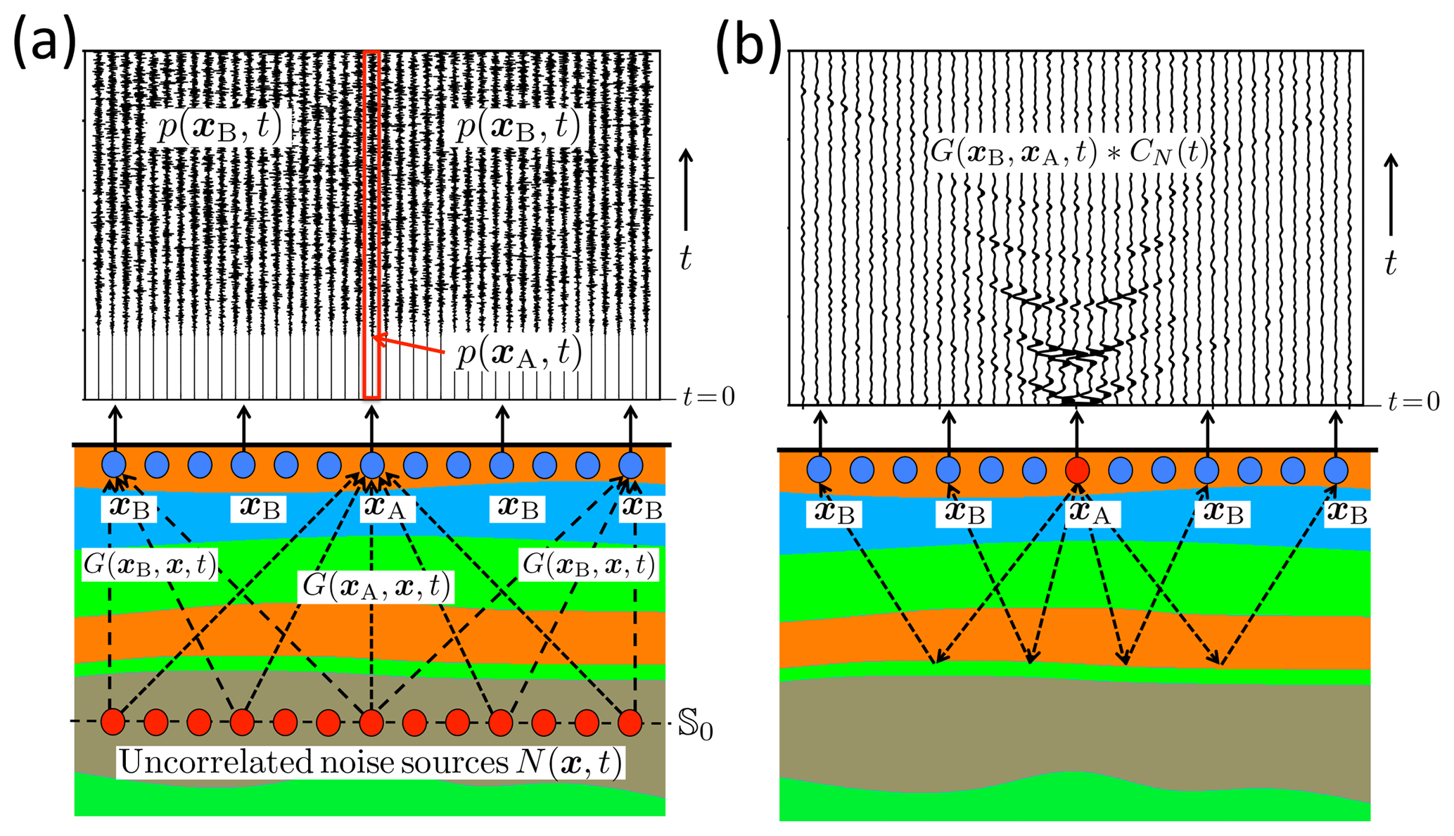
Figure 5 Seismic interferometry with body waves in a layered medium. The upper boundary is a free surface. (a) Noise observed by receivers just below the surface, due to uncorrelated noise sources in the subsurface (only the first 5 s of approximately 5 min of noise registrations are shown). (b) Retrieved reflection response, including multiple reflections.

According to Eqs. (16) and (17), it is assumed that the fields p(x_A,t) and p(x_B,t) are the responses to noise sources on a closed surface 𝕊. However, in the example in Fig. 4, the noise field is emitted into the medium from a finite open surface 𝕊₀. A consequence of this discrepancy is that the retrieved response in Fig. 4b lacks the acausal term $G({\mathit{x}}_{\mathrm{B}},{\mathit{x}}_{\mathrm{A}},-t)*C_N\left(t\right)$. Moreover, the causal term $G({\mathit{x}}_{\mathrm{B}},{\mathit{x}}_{\mathrm{A}},t)*C_N\left(t\right)$ is blurred by scattering noise, which does not vanish with longer time-averaging. According to Eqs. (16), (17) and (21), the retrieved response would contain the causal and acausal terms and the scattering noise would vanish if the noise field was emitted from a closed surface and the recorded fields at x_A and x_B were correlated for a long enough time.

Figure 4 is representative of seismic surface-wave interferometry (Campillo and Paul, 2003; Sabra et al., 2005b; Shapiro and Campillo, 2004; Bensen et al., 2007), in which case Fig. 4a should be interpreted as a plan view, with the noise signals representing microseisms, 𝕊₀ representing a coast line and the Green's functions representing the fundamental mode of surface waves (with additional effort, higher-mode surface waves can be retrieved as well – Halliday and Curtis, 2008; Kimman and Trampert, 2010; Kimman et al., 2012; van Dalen et al., 2014). The retrieved surface-wave Green's functions are typically used for tomographic imaging (Sabra et al., 2005a; Shapiro et al., 2005; Bensen et al., 2008; Lin et al., 2009). Seismic interferometry can also be used for reflection imaging of the Earth's crust with body waves. Because the scattering mechanism is very different, we discuss a second example to illustrate seismic interferometry with body waves. Figure 5a shows the same layered medium as Fig. 3a, but this time with noise sources at 𝕊₀ in the subsurface and with the upper surface being a free surface. For this situation the part of the closed-surface integral over the free surface in Eq. (6) vanishes. Hence, the closed surface integrals in Eqs. (16) and (17) can be replaced by open surface integrals over the noise sources in the subsurface in Fig. 5a. The responses to these noise sources, shown in the upper part of Fig. 5a, are recorded by receivers below the free surface. For p(x_A,t) we take the central trace (indicated by the red box) and for p(x_B,t) (with variable x_B) all other traces. We apply Eq. (21) to obtain the virtual-source response $G({\mathit{x}}_{\mathrm{B}},{\mathit{x}}_{\mathrm{A}},t)*C_N\left(t\right)$ and its time-reversal $G({\mathit{x}}_{\mathrm{B}},{\mathit{x}}_{\mathrm{A}},-t)*C_N\left(t\right)$ for a fixed virtual source at x_A and receivers at variable x_B. The causal part is shown in Fig. 5b. In agreement with the theory, this is the full reflection response of the layered medium, including multiple reflections. Applications of reflection-response retrieval from ambient noise range from the shallow subsurface to the global scale (Chaput and Bostock, 2007; Draganov et al., 2009, 2013; Forghani and Snieder, 2010; Ryberg, 2011; Ruigrok et al., 2012; Tonegawa et al., 2013; Panea et al., 2014; Boué et al., 2014; Boullenger et al., 2015; Oren and Nowack, 2017; Almagro Vidal et al., 2018). As body waves in ambient noise are usually weak in comparison with surface waves, much effort is spent on recovering the body waves from behind the surface waves. Reflection responses retrieved by body-wave interferometry are typically used for reflection imaging.

For both methods discussed here (surface-wave interferometry and body-wave interferometry) we assumed that the noise sources are regularly distributed along a part of 𝕊 and that they all have the same autocorrelation function. In many practical situations the source distribution is irregular, and the autocorrelations are different for different sources. Several approaches have been developed to account for these issues, such as iterative correlation (Stehly et al., 2008), multidimensional deconvolution (Wapenaar and van der Neut, 2010; van der Neut et al., 2011), directional balancing (Curtis and Halliday, 2010a) and generalized interferometry, circumventing Green's function retrieval (Fichtner et al., 2017).

2.4 Back propagation

Given a wave field observed at the surface of a medium, the field inside the medium can be obtained by back propagation (Schneider, 1978; Berkhout, 1982; Fischer and Langenberg, 1984; Wiggins, 1984; Langenberg et al., 1986). Because back propagation implies retrieving a 3-D field inside a volume from a 2-D field at a surface, it is also known as holography (Porter and Devaney, 1982; Lindsey and Braun, 2004). Figure 6 illustrates the principle. In Fig. 6a, the field at the finite open surface 𝕊₀ due to a source at x_A inside a layered medium (the same medium as in Figs. 3 and 5) is back propagated to an arbitrary point x_B inside the medium by the time-reversed direct arrival of the Green's function, $G_{\mathrm{d}}(\mathit{x},{\mathit{x}}_{\mathrm{B}},-t)$. Figure 6b shows $G_{\mathrm{d}}(\mathit{x},{\mathit{x}}_{\mathrm{B}},-t)$ (for fixed x_B) and a snapshot of the back propagated field at time instant t₁>0 for all x_B. Note that above the source (which is located at x_A) the primary upgoing field coming from the source is clearly retrieved. However, the field below the source is not retrieved. Moreover, several artefacts are present because multiple reflections between the layer interfaces are not accounted for.

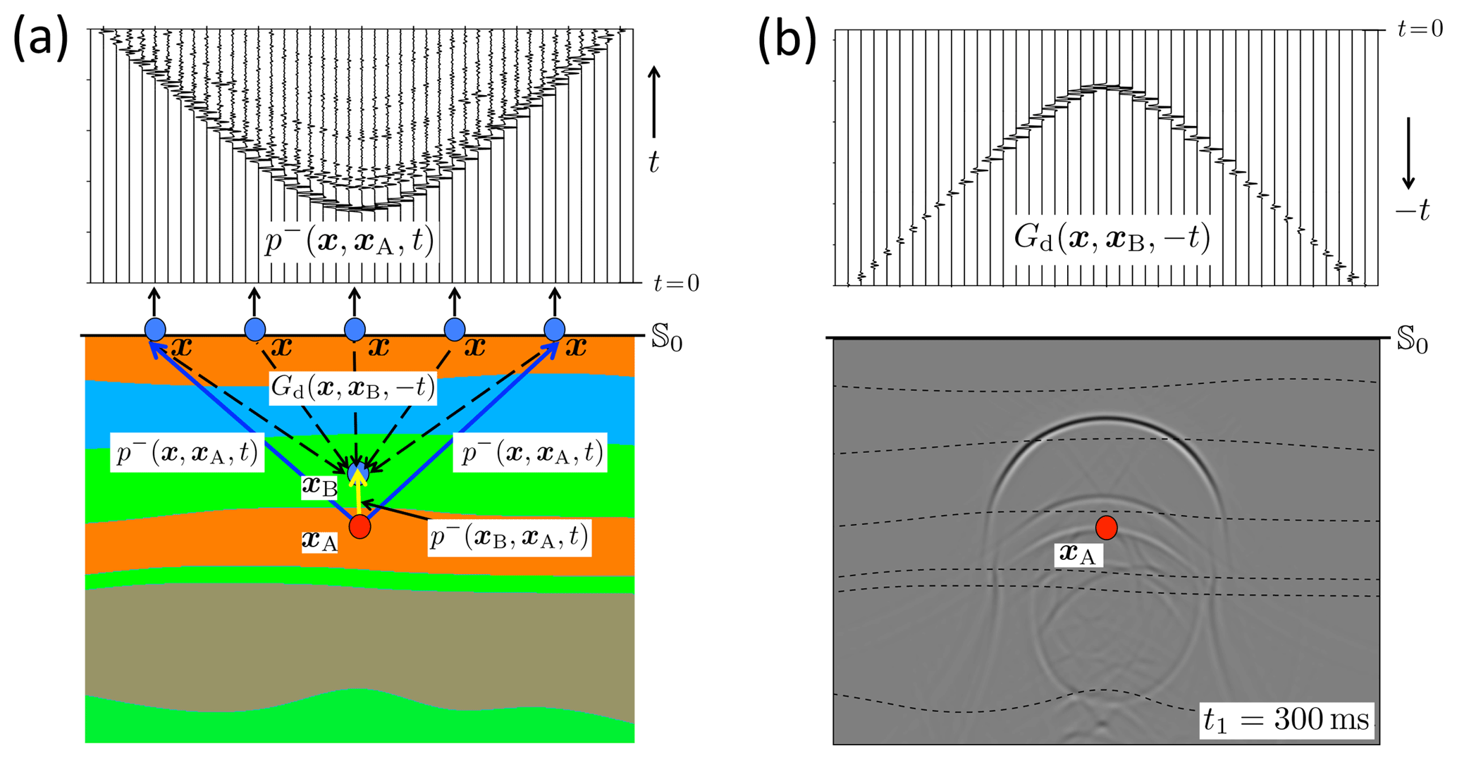
Figure 6 Principle of back propagation. (a) The upgoing wave field $p^{-}(\mathit{x},{\mathit{x}}_{\mathrm{A}},t)$ at the surface 𝕊₀ and illustration of its back propagation to x_B inside the medium. (b) The back propagation operator $G_{\mathrm{d}}(\mathit{x},{\mathit{x}}_{\mathrm{B}},-t)$ (for variable x along 𝕊₀ and fixed x_B) and a snapshot of the back propagated wave field $p^{-}({\mathit{x}}_{\mathrm{B}},{\mathit{x}}_{\mathrm{A}},t)$ at t₁=300 ms for all x_B.

Back propagation is conceptually different from time-reversal acoustics. In time-reversal acoustics the observed wave field is reversed in time and (physically or numerically) emitted into the medium, whereas in back propagation the original observed wave field is numerically back-propagated through the medium by a time-reversed Green's function. Despite this conceptual difference (time reversal of the wave field versus time reversal of the propagation operator), it is not surprising that these methods are very similar from a mathematical point of view.

Figure 7 (a) Principle of source–receiver redatuming. (b) Reflectivity image $r\left({\mathit{x}}_{\mathrm{A}}\right)\approx p^{-,+}({\mathit{x}}_{\mathrm{A}},{\mathit{x}}_{\mathrm{A}},t=\mathrm{0})$ for all x_A. The red arrows indicate erroneously imaged multiples.

A quantitative discussion of back propagation follows from Eq. (7). By interchanging x_A and x_B and multiplying both sides by the spectrum s(ω) of the source at x_A, we obtain

$$\begin{array}{ll}{\displaystyle }& {\displaystyle }{G}_{\mathrm{h}}({\mathit{x}}_{\mathrm{B}},{\mathit{x}}_{\mathrm{A}},\mathit{\omega })s\left(\mathit{\omega }\right)\\ \text{(22)}& {\displaystyle }& {\displaystyle }=-\mathrm{2}\underset{\mathbb{S}}{\oint }{\displaystyle \frac{\mathrm{1}}{i\mathit{\omega }{\mathit{\rho }}_{\mathrm{0}}}}\mathit{\left\{}{\partial }_i{G}^{*}\right(\mathit{x},{\mathit{x}}_{\mathrm{B}},\mathit{\omega }\left)\mathit{\right\}}G(\mathit{x},{\mathit{x}}_{\mathrm{A}},\mathit{\omega })s\left(\mathit{\omega }\right)n_i\mathrm{d}\mathit{x}.\end{array}$$

Here $G(\mathit{x},{\mathit{x}}_{\mathrm{A}},\mathit{\omega })s\left(\mathit{\omega }\right)$ stands for the observed field $p(\mathit{x},{\mathit{x}}_{\mathrm{A}},\mathit{\omega })$ at the surface 𝕊, and $-\frac{\mathrm{2}}{i\mathit{\omega }{\mathit{\rho }}_{\mathrm{0}}}{\partial }_i{G}^{*}(\mathit{x},{\mathit{x}}_{\mathrm{B}},\mathit{\omega })n_i$ is the back propagation operator, both in the frequency domain. Hence, in theory the exact field $G_{\mathrm{h}}({\mathit{x}}_{\mathrm{B}},{\mathit{x}}_{\mathrm{A}},\mathit{\omega })s\left(\mathit{\omega }\right)$ can be obtained at any x_B inside the medium. Because in practical situations the field $p(\mathit{x},{\mathit{x}}_{\mathrm{A}},\mathit{\omega })$ is only observed at a finite part 𝕊₀ of the surface, approximations arise in practice when the closed surface 𝕊 is replaced by 𝕊₀. One of the consequences is that multiple reflections are not handled correctly. A detailed analysis (Wapenaar et al., 1989) shows that the primary arrival of the upgoing wave field $p^{-}({\mathit{x}}_{\mathrm{B}},{\mathit{x}}_{\mathrm{A}},\mathit{\omega })=G^{-}({\mathit{x}}_{\mathrm{B}},{\mathit{x}}_{\mathrm{A}},\mathit{\omega })s\left(\mathit{\omega }\right)$ is reasonably accurately retrieved with the following approximation of Eq. (22):

$$\begin{array}{}\text{(23)}& p^{-}({\mathit{x}}_{\mathrm{B}},{\mathit{x}}_{\mathrm{A}},\mathit{\omega })\approx \underset{{\mathbb{S}}_{\mathrm{0}}}{\int }{F}_{\mathrm{d}}^{+}(\mathit{x},{\mathit{x}}_{\mathrm{B}},\mathit{\omega })p^{-}(\mathit{x},{\mathit{x}}_{\mathrm{A}},\mathit{\omega })\mathrm{d}\mathit{x}.\end{array}$$

Here the back propagation operator $F_{\mathrm{d}}^{+}(\mathit{x},{\mathit{x}}_{\mathrm{B}},\mathit{\omega })$, also known as the focusing operator, is defined as

$$\begin{array}{}\text{(24)}& F_{\mathrm{d}}^{+}(\mathit{x},{\mathit{x}}_{\mathrm{B}},\mathit{\omega })={\displaystyle \frac{\mathrm{2}}{i\mathit{\omega }{\mathit{\rho }}_{\mathrm{0}}}}{\partial }_{\mathrm{3}}{G}_{\mathrm{d}}^{*}(\mathit{x},{\mathit{x}}_{\mathrm{B}},\mathit{\omega }),\end{array}$$

where we used $n_{\mathrm{3}}=-\mathrm{1}$ at 𝕊₀, considering that the positive x₃ axis is pointing downward. Equations (23) and (24) represent the common approach to back propagation for many applications in seismic imaging and inversion. It works well for primary waves in media with low contrasts, but it breaks down when the contrasts are strong and multiple reflections between the layer interfaces cannot be ignored. In Sect. 3.3 we discuss a modified approach to back-propagation which enables the recovery of the full wave field $p({\mathit{x}}_{\mathrm{B}},{\mathit{x}}_{\mathrm{A}},\mathit{\omega })$, including the multiple reflections, inside the medium (also below the source at x_A) and which also suppresses artefacts like those in Fig. 6b in a data-driven way.

2.5 Source–receiver redatuming and imaging by double focusing

In the previous section we discussed back propagation of $p^{-}(\mathit{x},{\mathit{x}}_{\mathrm{A}},\mathit{\omega })$, which is the response to a source at x_A inside the medium, observed at x at the surface. Here we extend this process for the situation in which both the sources and receivers are located at the surface. To this end, we first adapt Eqs. (23) and (24). We replace 𝕊₀ with ${\mathbb{S}}_{\mathrm{0}}^{\prime }$ (just above 𝕊₀), x with ${\mathit{x}}^{\prime }\in {\mathbb{S}}_{\mathrm{0}}^{\prime }$, x_A with x∈𝕊₀ and x_B with x_A, and we add an extra superscript (+) to the wave fields (explained below), which yields

$$\begin{array}{}\text{(25)}& p^{-,+}({\mathit{x}}_{\mathrm{A}},\mathit{x},\mathit{\omega })\approx \underset{{\mathbb{S}}_{\mathrm{0}}^{\prime }}{\int }{F}_{\mathrm{d}}^{+}({\mathit{x}}^{\prime },{\mathit{x}}_{\mathrm{A}},\mathit{\omega })p^{-,+}({\mathit{x}}^{\prime },\mathit{x},\mathit{\omega })\mathrm{d}{\mathit{x}}^{\prime },\end{array}$$

with

$$\begin{array}{}\text{(26)}& F_{\mathrm{d}}^{+}({\mathit{x}}^{\prime },{\mathit{x}}_{\mathrm{A}},\mathit{\omega })={\displaystyle \frac{\mathrm{2}}{i\mathit{\omega }{\mathit{\rho }}_{\mathrm{0}}}}{\partial }_{\mathrm{3}}^{\prime }{G}_{\mathrm{d}}^{*}({\mathit{x}}^{\prime },{\mathit{x}}_{\mathrm{A}},\mathit{\omega }).\end{array}$$

Here ${\partial }_{\mathrm{3}}^{\prime }$ stands for differentiation with respect to $x_{\mathrm{3}}^{\prime }$. In Eq. (25), $p^{-,+}({\mathit{x}}^{\prime },\mathit{x},\mathit{\omega })=G^{-,+}({\mathit{x}}^{\prime },\mathit{x},\mathit{\omega })s\left(\mathit{\omega }\right)$ represents the reflection data at the surface. The first superscript (−) denotes that the field is upgoing at x^′; the second superscript (+) denotes that the source at x emits downgoing waves. Furthermore, $p^{-,+}({\mathit{x}}_{\mathrm{A}},\mathit{x},\mathit{\omega })=G^{-,+}({\mathit{x}}_{\mathrm{A}},\mathit{x},\mathit{\omega })s\left(\mathit{\omega }\right)$ is the back propagated upgoing field at x_A. Applying source–receiver reciprocity on both sides of Eq. (25) we obtain

$$\begin{array}{}\text{(27)}& p^{-,+}(\mathit{x},{\mathit{x}}_{\mathrm{A}},\mathit{\omega })\approx \underset{{\mathbb{S}}_{\mathrm{0}}^{\prime }}{\int }{p}^{-,+}(\mathit{x},{\mathit{x}}^{\prime },\mathit{\omega })F_{\mathrm{d}}^{+}({\mathit{x}}^{\prime },{\mathit{x}}_{\mathrm{A}},\mathit{\omega })\mathrm{d}{\mathit{x}}^{\prime }.\end{array}$$

The receiver for upgoing waves at x_A has turned into a source for downgoing waves at x_A, and so on. Hence, Eq. (27) back propagates the sources from x^′ on ${\mathbb{S}}_{\mathrm{0}}^{\prime }$ to x_A. Substituting this into Eq. (23), with p⁻ replaced by $p^{-,+}$ on both sides, gives

$$\begin{array}{ll}{\displaystyle }& {\displaystyle }{p}^{-,+}({\mathit{x}}_{\mathrm{B}},{\mathit{x}}_{\mathrm{A}},\mathit{\omega })\\ \text{(28)}& {\displaystyle }& {\displaystyle }\approx \underset{{\mathbb{S}}_{\mathrm{0}}}{\int }\underset{{\mathbb{S}}_{\mathrm{0}}^{\prime }}{\int }{F}_{\mathrm{d}}^{+}(\mathit{x},{\mathit{x}}_{\mathrm{B}},\mathit{\omega })p^{-,+}(\mathit{x},{\mathit{x}}^{\prime },\mathit{\omega })F_{\mathrm{d}}^{+}({\mathit{x}}^{\prime },{\mathit{x}}_{\mathrm{A}},\mathit{\omega })\mathrm{d}{\mathit{x}}^{\prime }\mathrm{d}\mathit{x}.\end{array}$$

Here $p^{-,+}(\mathit{x},{\mathit{x}}^{\prime },\mathit{\omega })$ represents the reflection response at the surface (illustrated by the blue arrows in Fig. 7a). Similarly, $p^{-,+}({\mathit{x}}_{\mathrm{B}},{\mathit{x}}_{\mathrm{A}},\mathit{\omega })$ denotes the reflection response to a source for downgoing waves at x_A, observed by a receiver for upgoing waves at x_B (illustrated by the yellow arrows in Fig. 7a). According to Eq. (28), it is obtained by back propagating sources from x^′ to x_A with operator $F_{\mathrm{d}}^{+}({\mathit{x}}^{\prime },{\mathit{x}}_{\mathrm{A}},\mathit{\omega })$ and receivers from x to x_B with operator $F_{\mathrm{d}}^{+}(\mathit{x},{\mathit{x}}_{\mathrm{B}},\mathit{\omega })$, indicated by the dashed arrows in Fig. 7a. In the exploration community this process is called (source–receiver) redatuming (Berkhout, 1982; Berryhill, 1984) and is closely related to source–receiver interferometry (Curtis and Halliday, 2010b). For the elastodynamic extension, see Kuo and Dai (1984), Wapenaar and Berkhout (1989) and Hokstad (2000).

The redatumed response $p^{-,+}({\mathit{x}}_{\mathrm{B}},{\mathit{x}}_{\mathrm{A}},\mathit{\omega })$ can be used for reflectivity imaging by setting x_B equal to x_A and selecting the t=0 component in the time domain, as follows:

$$\begin{array}{}\text{(29)}& r\left({\mathit{x}}_{\mathrm{A}}\right)\approx p^{-,+}({\mathit{x}}_{\mathrm{A}},{\mathit{x}}_{\mathrm{A}},t=\mathrm{0})={\displaystyle \frac{\mathrm{1}}{\mathrm{2}\mathit{\pi }}}\underset{-\mathrm{\infty }}{\overset{\mathrm{\infty }}{\int }}{p}^{-,+}({\mathit{x}}_{\mathrm{A}},{\mathit{x}}_{\mathrm{A}},\mathit{\omega })\mathrm{d}\mathit{\omega }.\end{array}$$

The combined process (Eqs. 28 and 29) comprises imaging by double focusing (Berkhout, 1982; Wiggins, 1984; Bleistein, 1987; Berkhout and Wapenaar, 1993; Blondel et al., 2018), because it involves the application of the focusing operator $F_{\mathrm{d}}^{+}(\mathit{x},{\mathit{x}}_{\mathrm{A}},\mathit{\omega })$ twice. By taking the focal point x_A variable, a reflectivity image of the entire region of interest is obtained. Figure 7b shows an image of the same layered medium as considered in previous examples obtained in this way. Note that the interfaces are clearly imaged, but also that significant artefacts are present because multiple reflections are not correctly handled (indicated by the red arrows). In Sect. 3.4 and 3.5 we discuss more rigorous approaches to source–receiver redatuming and imaging by double focusing, which account for multiple reflections in a data-driven way.

3 Theory and applications of a modified single-sided wave field representation

The applications of Green's theorem, discussed in Sect. 2, are all derived from the classical homogeneous Green's function representation. This representation is exact, but it involves an integral over a closed surface. In many practical situations the medium of interest is only accessible from one side, which implies that the integration can only be carried out over an open surface. This induces approximations, of which the incomplete treatment of multiple reflections is the most significant one. In the following we discuss a modification of the homogeneous Green's function representation which involves an integral over an open surface and yet accounts for all multiple reflections. We call this modified representation the single-sided homogeneous Green's function representation. Next, we discuss how it can be used to improve several of the applications discussed in Sect. 2.

Figure 8 The focusing function $f_{\mathrm{1}}(\mathit{x},{\mathit{x}}_{\mathrm{A}},t)$ in a truncated version of the actual medium.

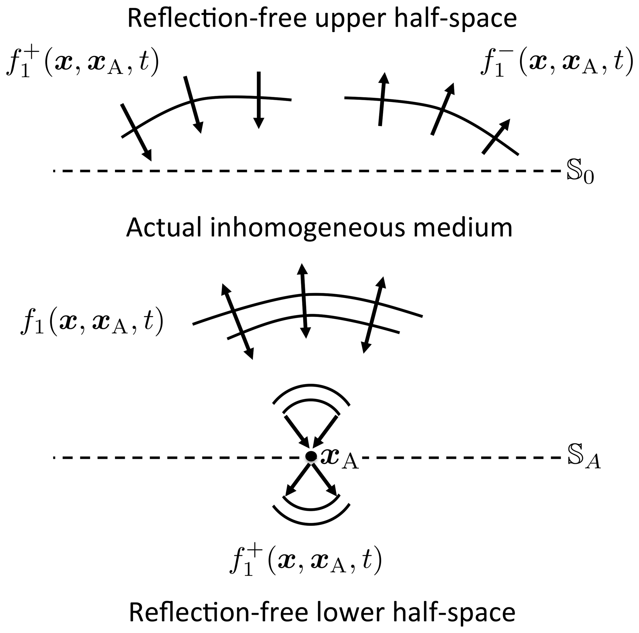
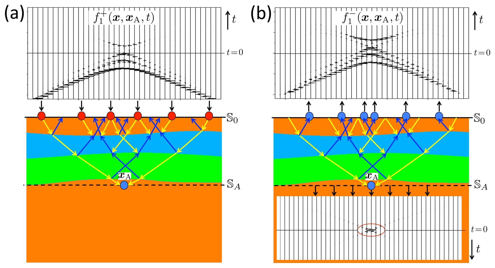
Figure 9 Numerical example of the focusing function. (a) Emission of the downgoing part of the focusing function from 𝕊₀ into a truncated version of the actual medium. (b) Responses at 𝕊₀ and 𝕊_A.

3.1 Single-sided homogeneous Green's function representation

The classical homogeneous Green's function representations (Eqs. 6 and 7) are entirely formulated in terms of Green's functions and their time reversals. A Green's function is the causal response to a source at a specific position in space, say at x_A. A time-reversed Green's function can be seen as a focusing function which focuses at x_A. However, this only holds when it converges to x_A equally from all directions, which can be achieved by emitting it into the medium from a closed surface. For practical situations we need another type of focusing function, which, when emitted into the medium from a single surface, focuses at x_A. We introduce the focusing function using Fig. 8. This figure shows a truncated version of the medium, which is identical to the actual medium between the upper surface 𝕊₀ and the focal plane 𝕊_A (the plane which contains the focal point x_A), but it is reflection free above 𝕊₀ and below 𝕊_A (here “reflection free” means that the medium parameters do not vary in the vertical direction). We call the focusing function $f_{\mathrm{1}}(\mathit{x},{\mathit{x}}_{\mathrm{A}},t)$. In the reflection-free half-space above 𝕊₀ the focusing function consists of both a downgoing and upgoing part, according to

$$\begin{array}{}\text{(30)}& f_{\mathrm{1}}(\mathit{x},{\mathit{x}}_{\mathrm{A}},t)=f_{\mathrm{1}}^{+}(\mathit{x},{\mathit{x}}_{\mathrm{A}},t)+f_{\mathrm{1}}^{-}(\mathit{x},{\mathit{x}}_{\mathrm{A}},t),\end{array}$$

where the superscripts + and − indicate downgoing and upgoing, respectively. The downgoing part $f_{\mathrm{1}}^{+}(\mathit{x},{\mathit{x}}_{\mathrm{A}},t)$ is shaped such that $f_{\mathrm{1}}(\mathit{x},{\mathit{x}}_{\mathrm{A}},t)$ focuses at x_A at t=0, and continues as a diverging downgoing field into the reflection-free half-space below 𝕊_A. The upgoing part of the focusing function in the upper half-space, $f_{\mathrm{1}}^{-}(\mathit{x},{\mathit{x}}_{\mathrm{A}},t)$, is defined as the reflection response of the truncated medium to the downgoing focusing function $f_{\mathrm{1}}^{+}(\mathit{x},{\mathit{x}}_{\mathrm{A}},t)$. The focusing property at the focal plane 𝕊_A can be formulated as

$$\begin{array}{}\text{(31)}& \mathit{\delta }({\mathit{x}}_{\mathrm{H},\mathrm{A}}^{\prime }-{\mathit{x}}_{\mathrm{H},\mathrm{A}})\mathit{\delta }\left(t\right)=\underset{{\mathbb{S}}_{\mathrm{0}}}{\int }\mathcal{T}({\mathit{x}}_{\mathrm{A}}^{\prime },\mathit{x},t)*f_{\mathrm{1}}^{+}(\mathit{x},{\mathit{x}}_{\mathrm{A}},t)\mathrm{d}\mathit{x},\end{array}$$

where $\mathcal{T}({\mathit{x}}_{\mathrm{A}}^{\prime },\mathit{x},t)$ is the transmission response of the truncated medium between 𝕊₀ and 𝕊_A, and x_H,A and ${\mathit{x}}_{\mathrm{H},\mathrm{A}}^{\prime }$ are the horizontal coordinates of x_A and ${\mathit{x}}_{\mathrm{A}}^{\prime }$ (both at 𝕊_A), respectively (the precise definition of $\mathcal{T}({\mathit{x}}_{\mathrm{A}}^{\prime },\mathit{x},t)$ is given in Appendix A of Wapenaar et al., 2014a). In physical terms, Eq. (31) formulates the emission of $f_{\mathrm{1}}^{+}(\mathit{x},{\mathit{x}}_{\mathrm{A}},t)$ from 𝕊₀ into the truncated medium, leading to a focus at x_A. In mathematical terms, Eq. (31) defines $f_{\mathrm{1}}^{+}(\mathit{x},{\mathit{x}}_{\mathrm{A}},t)$ as the inverse of the transmission response $\mathcal{T}({\mathit{x}}_{\mathrm{A}}^{\prime },\mathit{x},t)$. Because the evanescent part of the transmission response cannot be inverted in a stable way, in practice the focusing function, and hence the focus at 𝕊_A, is band-limited.

The focusing function is illustrated using a numerical example in Fig. 9. Figure 9a shows how the downgoing part of the focusing function, $f_{\mathrm{1}}^{+}(\mathit{x},{\mathit{x}}_{\mathrm{A}},t)$, is emitted from x at 𝕊₀ into the medium. The first event (at negative time) propagates downward toward the focal point x_A, indicated by the outer yellow rays (represented using arrows). On its path to the focal point it is reflected at layer interfaces, indicated by the blue rays. During upward propagation, these blue rays meet new yellow rays (coming from the later events of the focusing function), in such a way that effectively no downward reflection takes place at the layer interfaces, and so on. Hence, only the first event of the focusing function reaches the focal depth, where it focuses at x_A. Figure 9b shows the responses to the focusing function, at 𝕊₀ and 𝕊_A. The response at 𝕊₀ is the upgoing part of the focusing function, $f_{\mathrm{1}}^{-}(\mathit{x},{\mathit{x}}_{\mathrm{A}},t)$; the response at 𝕊_A is the band-limited focused field.

Given the focusing function for a focal point at x_A and the Green's function for a source at x_B, the single-sided representation of the homogeneous Green's function in the frequency domain reads (Wapenaar et al., 2016a)

$$\begin{array}{ll}{\displaystyle }{G}_{\mathrm{h}}({\mathit{x}}_{\mathrm{B}},{\mathit{x}}_{\mathrm{A}},\mathit{\omega })& {\displaystyle }=\mathrm{2}\underset{{\mathbb{S}}_{\mathrm{0}}}{\int }{\displaystyle \frac{\mathrm{1}}{\mathit{\omega }\mathit{\rho }\left(\mathit{x}\right)}}\left(\mathit{\right\{}{\partial }_i{G}_{\mathrm{h}}(\mathit{x},{\mathit{x}}_{\mathrm{B}},\mathit{\omega })\mathit{\left\}}\mathrm{\Im }\mathit{\right\{}{f}_{\mathrm{1}}(\mathit{x},{\mathit{x}}_{\mathrm{A}},\mathit{\omega })\mathit{\}}\\ \text{(32)}& {\displaystyle }& {\displaystyle }-G_{\mathrm{h}}(\mathit{x},{\mathit{x}}_{\mathrm{B}},\mathit{\omega })\mathrm{\Im }\mathit{\left\{}{\partial }_i{f}_{\mathrm{1}}\right(\mathit{x},{\mathit{x}}_{\mathrm{A}},\mathit{\omega }\left)\mathit{\right\}})n_i\mathrm{d}\mathit{x},\end{array}$$

where ℑ denotes the imaginary part. The derivation can be found in the Supplement, Sect. S2.2 (a similar single-sided representation for vectorial wave fields is derived by Wapenaar et al., 2016b, and illustrated using numerical examples by Reinicke and Wapenaar, 2019). In Eq. (32), 𝕊₀ may be a curved surface. Moreover, the actual medium, in which the Green's function is defined, may be inhomogeneous above 𝕊₀ (in addition to being inhomogeneous below 𝕊₀). Note the resemblance with the classical representation of Eq. (6). Unlike the classical representation, which is exact, Eq. (32) holds under the assumption that evanescent waves can be neglected. When 𝕊₀ is horizontal and the medium above 𝕊₀ is homogeneous (for the Green's function as well as for the focusing function), this representation may be approximated by

$$\begin{array}{ll}{\displaystyle }{G}_{\mathrm{h}}({\mathit{x}}_{\mathrm{B}},{\mathit{x}}_{\mathrm{A}},\mathit{\omega })& {\displaystyle }=\mathrm{4}\mathrm{\Re }\underset{{\mathbb{S}}_{\mathrm{0}}}{\int }{\displaystyle \frac{\mathrm{1}}{i\mathit{\omega }{\mathit{\rho }}_{\mathrm{0}}}}G(\mathit{x},{\mathit{x}}_{\mathrm{B}},\mathit{\omega }){\partial }_{\mathrm{3}}\left(f_{\mathrm{1}}^{+}\right(\mathit{x},{\mathit{x}}_{\mathrm{A}},\mathit{\omega })\\ \text{(33)}& {\displaystyle }& {\displaystyle }-\mathit{\left\{}{f}_{\mathrm{1}}^{-}\right(\mathit{x},{\mathit{x}}_{\mathrm{A}},\mathit{\omega }\left){\mathit{\}}}^{*}\right)\mathrm{d}\mathit{x}\end{array}$$

(Van der Neut et al., 2017). For the derivation, see the Supplement, Sect. S2.3. For the decomposed Green's function $G^{-,+}({\mathit{x}}_{\mathrm{B}},{\mathit{x}}_{\mathrm{A}},\mathit{\omega })$, introduced in Sect. 2.5, we have the following representation (by combining Eqs. S31 and S38 of the Supplement)

$$\begin{array}{ll}{\displaystyle }{G}^{-,+}& {\displaystyle }({\mathit{x}}_{\mathrm{B}},{\mathit{x}}_{\mathrm{A}},\mathit{\omega })\\ {\displaystyle }& {\displaystyle }=\mathrm{2}\underset{{\mathbb{S}}_{\mathrm{0}}}{\int }{\displaystyle \frac{\mathrm{1}}{i\mathit{\omega }{\mathit{\rho }}_{\mathrm{0}}}}{G}^{-,+}(\mathit{x},{\mathit{x}}_{\mathrm{B}},\mathit{\omega }){\partial }_{\mathrm{3}}{f}_{\mathrm{1}}^{+}(\mathit{x},{\mathit{x}}_{\mathrm{A}},\mathit{\omega })\mathrm{d}\mathit{x}\\ \text{(34)}& {\displaystyle }& {\displaystyle }-\mathit{\chi }\left({\mathit{x}}_{\mathrm{B}}\right)f_{\mathrm{1}}^{-}({\mathit{x}}_{\mathrm{B}},{\mathit{x}}_{\mathrm{A}},\mathit{\omega }),\end{array}$$

where χ is the characteristic function of the medium enclosed by 𝕊₀ and 𝕊_A. It is defined as

$$\begin{array}{}\text{(35)}& \mathit{\chi }\left({\mathit{x}}_{\mathrm{B}}\right)=\left\{\begin{array}{ll}\mathrm{1},& \text{for }{\mathit{x}}_{\mathrm{B}}\text{ between }{\mathbb{S}}_{\mathrm{0}}\text{ and }{\mathbb{S}}_{\mathrm{A}},\\ {\displaystyle \frac{\mathrm{1}}{\mathrm{2}}},& \text{for }{\mathit{x}}_{\mathrm{B}}\text{ on }\mathbb{S}={\mathbb{S}}_{\mathrm{0}}\cup {\mathbb{S}}_{\mathrm{A}},\\ \mathrm{0},& \text{for }{\mathit{x}}_{\mathrm{B}}\text{ outside }\mathbb{S}.\end{array}\right.\end{array}$$

In many practical situations 𝕊₀ is a free surface, which means that the assumption of a homogeneous medium above 𝕊₀ is not fulfilled. A free surface gives rise to surface-related multiple reflections. These can be removed by a process called surface-related multiple elimination (Verschuur et al., 1992). Applying this process is equivalent to replacing the free surface with a transparent surface and a homogeneous half-space above this surface (Fokkema and van den Berg, 1993; van Borselen et al., 1996). Hence, when 𝕊₀ is a free surface, Eqs. (33) and (34) hold for the situation after surface-related multiple elimination.

The representations of Eqs. (33) and (34) form the starting point for modifying several of the applications discussed in Sect. 2. These methods, which will be discussed in the subsequent sections, have the fact in common that they make use of focusing functions. As stated earlier, the focusing function $f_{\mathrm{1}}^{+}(\mathit{x},{\mathit{x}}_{\mathrm{A}},t)$ for x at 𝕊₀ is the inverse of the transmission response of the truncated medium between 𝕊₀ and 𝕊_A. Hence, when a detailed model of the medium between these depth levels is available, its transmission response can be numerically modeled and $f_{\mathrm{1}}^{+}(\mathit{x},{\mathit{x}}_{\mathrm{A}},t)$ can be obtained by inverting this transmission response. Next, $f_{\mathrm{1}}^{-}(\mathit{x},{\mathit{x}}_{\mathrm{A}},t)$ can be obtained by applying the reflection response of the truncated medium to $f_{\mathrm{1}}^{+}(\mathit{x},{\mathit{x}}_{\mathrm{A}},t)$. This is obviously a model-driven approach. Conversely, when the reflection response of the actual medium is available at 𝕊₀, the focusing functions $f_{\mathrm{1}}^{+}(\mathit{x},{\mathit{x}}_{\mathrm{A}},t)$ and $f_{\mathrm{1}}^{-}(\mathit{x},{\mathit{x}}_{\mathrm{A}},t)$ for x at 𝕊₀ can be retrieved from this reflection response using a 3-D extension of the Marchenko method (Wapenaar et al., 2014a; Slob et al., 2014). This method needs an initial estimate of $f_{\mathrm{1}}^{+}(\mathit{x},{\mathit{x}}_{\mathrm{A}},t)$, for which one could use the inverse of the direct arrival of the transmission response. This requires only a smooth model of the medium between 𝕊₀ and 𝕊_A. In practice, the back propagating direct arrival of the Green's function, $G_{\mathrm{d}}(\mathit{x},{\mathit{x}}_{\mathrm{A}},-t)$, is usually taken as initial estimate. Because the Marchenko method uses the reflection response (obtained from reflection measurements at the surface 𝕊₀) and a smooth model of the medium, it is a data-driven approach for retrieving the focusing functions. One of the underlying assumptions of the Marchenko method is that the Green's functions and the focusing functions are separable in time. This assumption is satisfied for layered media with moderate lateral variations (like in Fig. 3), considering moderate horizontal source–receiver offsets; it breaks down for strongly scattering media (like in Fig. 2). In the latter case the Marchenko method is only approximately valid, but despite the approximation it can still lead to better images than standard imaging methods (Wapenaar et al., 2014b). A further discussion of the 3-D Marchenko method is beyond the scope of this paper.

Figure 10 Time-reversal acoustics in a layered medium. (a) Classical approach: emission of the time-reversed recordings from 𝕊₀ into the medium. (b) Emission of a modified field, defined by Eq. (36), into the medium. Note the improved focus.

3.2 Modified time-reversal acoustics

We discuss a modification of time-reversal acoustics. Assuming the focusing functions are available for x at 𝕊₀ (for example, from the Marchenko method), we define a new particle velocity field, according to

$$\begin{array}{ll}{\displaystyle }& {\displaystyle }{\widehat{v}}_{\mathrm{n}}^{*}(\mathit{x},{\mathit{x}}_{\mathrm{A}},\mathit{\omega })\\ \text{(36)}& {\displaystyle }& {\displaystyle }={\displaystyle \frac{\mathrm{1}}{i\mathit{\omega }{\mathit{\rho }}_{\mathrm{0}}}}{\partial }_{\mathrm{3}}\left(f_{\mathrm{1}}^{+}\right(\mathit{x},{\mathit{x}}_{\mathrm{A}},\mathit{\omega })-\mathit{\{}{f}_{\mathrm{1}}^{-}(\mathit{x},{\mathit{x}}_{\mathrm{A}},\mathit{\omega }){\mathit{\}}}^{*}\left)s\right(\mathit{\omega }),\end{array}$$

where for s(ω) we take a real-valued spectrum. Using this in Eq. (33) we obtain

$$\begin{array}{}\text{(37)}& G_{\mathrm{h}}({\mathit{x}}_{\mathrm{B}},{\mathit{x}}_{\mathrm{A}},\mathit{\omega })s\left(\mathit{\omega }\right)=\mathrm{4}\mathrm{\Re }\underset{{\mathbb{S}}_{\mathrm{0}}}{\int }G({\mathit{x}}_{\mathrm{B}},\mathit{x},\mathit{\omega }){\widehat{v}}_{\mathrm{n}}^{*}(\mathit{x},{\mathit{x}}_{\mathrm{A}},\mathit{\omega })\mathrm{d}\mathit{x}.\end{array}$$

In the time domain this becomes

$$\begin{array}{ll}{\displaystyle }{G}_{\mathrm{h}}({\mathit{x}}_{\mathrm{B}},{\mathit{x}}_{\mathrm{A}},t)*s\left(t\right)& {\displaystyle }=\mathrm{2}\underset{{\mathbb{S}}_{\mathrm{0}}}{\int }G({\mathit{x}}_{\mathrm{B}},\mathit{x},t)*{\widehat{v}}_{\mathrm{n}}(\mathit{x},{\mathit{x}}_{\mathrm{A}},-t)\mathrm{d}\mathit{x}\\ \text{(38)}& {\displaystyle }& {\displaystyle }+\mathrm{2}\underset{{\mathbb{S}}_{\mathrm{0}}}{\int }G({\mathit{x}}_{\mathrm{B}},\mathit{x},-t)*{\widehat{v}}_{\mathrm{n}}(\mathit{x},{\mathit{x}}_{\mathrm{A}},t)\mathrm{d}\mathit{x}.\end{array}$$

The first integral is the same as that in Eq. (10) (except that ${\widehat{v}}_{\mathrm{n}}$ is defined differently), whereas the second integral is the time reversal of the first one. For ultrasonic applications, assuming there are receivers at one or more x_B locations, the field ${\widehat{v}}_{\mathrm{n}}(\mathit{x},{\mathit{x}}_{\mathrm{A}},-t)$ can be emitted physically into the real medium and its response can be measured at x_B. The homogeneous Green's function is then obtained by superposing this response and its time reversal. For geophysical applications, the first integral can, at least in theory, be evaluated by numerically emitting the field ${\widehat{v}}_{\mathrm{n}}(\mathit{x},{\mathit{x}}_{\mathrm{A}},-t)$ into a model of the Earth. The superposition of this integral and its time-reversal gives the homogeneous Green's function. Following either one of these procedures, the result obtained at t=0 is shown in Fig. 10b. For comparison, Fig. 10a once more shows the classical time-reversal result of Fig. 3b. Note the different character of the fields v_n and ${\widehat{v}}_{\mathrm{n}}$ in the upper panels, which only have one event in common i.e., the time-reversed direct arrival. The snapshots at t=0 in the lower panels are also very different: the artefacts in Fig. 10a are almost entirely absent in Fig. 10b. The latter figure only shows a clear focus at x_A.

Obtaining an accurate focus as in Fig. 10b by numerically emitting the field ${\widehat{v}}_{\mathrm{n}}(\mathit{x},{\mathit{x}}_{\mathrm{A}},-t)$ into the Earth requires a very accurate model of the Earth, which should include accurate information on the position, structure and contrast of the layer interfaces. This requirement can be overcome by also retrieving the Green's function $G({\mathit{x}}_{\mathrm{B}},\mathit{x},t)$ in Eq. (38) using the Marchenko method and evaluating the integrals for all x_B. This is not discussed any further here. Alternative methods that do not require information about the layer interfaces are discussed in Sect. 3.3 to 3.5 and are illustrated using examples.

3.3 Modified back propagation

We modify the approach for back propagation. By interchanging x_A and x_B in Eq. (33) and multiplying both sides with a real-valued source spectrum s(ω), we obtain

$$\begin{array}{ll}{\displaystyle }p({\mathit{x}}_{\mathrm{B}},{\mathit{x}}_{\mathrm{A}},\mathit{\omega })& {\displaystyle }+p^{*}({\mathit{x}}_{\mathrm{B}},{\mathit{x}}_{\mathrm{A}},\mathit{\omega })\\ \text{(39)}& {\displaystyle }& {\displaystyle }=\mathrm{2}\mathrm{\Re }\underset{{\mathbb{S}}_{\mathrm{0}}}{\int }F(\mathit{x},{\mathit{x}}_{\mathrm{B}},\mathit{\omega })p(\mathit{x},{\mathit{x}}_{\mathrm{A}},\mathit{\omega })\mathrm{d}\mathit{x},\end{array}$$

with $p(\mathit{x},{\mathit{x}}_{\mathrm{A}},\mathit{\omega })=G(\mathit{x},{\mathit{x}}_{\mathrm{A}},\mathit{\omega })s\left(\mathit{\omega }\right)$ and

$$\begin{array}{}\text{(40)}& F(\mathit{x},{\mathit{x}}_{\mathrm{B}},\mathit{\omega })={\displaystyle \frac{\mathrm{2}}{i\mathit{\omega }{\mathit{\rho }}_{\mathrm{0}}}}{\partial }_{\mathrm{3}}\left(f_{\mathrm{1}}^{+}(\mathit{x},{\mathit{x}}_{\mathrm{B}},\mathit{\omega })-\mathit{\left\{}{f}_{\mathrm{1}}^{-}\right(\mathit{x},{\mathit{x}}_{\mathrm{B}},\mathit{\omega }){\mathit{\}}}^{*}\right).\end{array}$$

Note that the operator $F_{\mathrm{d}}^{+}(\mathit{x},{\mathit{x}}_{\mathrm{B}},\mathit{\omega })$ in Eq. (24) is an approximation of the operator $F(\mathit{x},{\mathit{x}}_{\mathrm{B}},\mathit{\omega })$ in Eq. (40). It is obtained by omitting the term $\mathit{\left\{}{f}_{\mathrm{1}}^{-}\right(\mathit{x},{\mathit{x}}_{\mathrm{B}},\mathit{\omega }){\mathit{\}}}^{*}$ and replacing the term $f_{\mathrm{1}}^{+}(\mathit{x},{\mathit{x}}_{\mathrm{B}},\mathit{\omega })$ by its initial estimate, i.e., the Fourier transform of the direct arrival of the Green's function, $G_{\mathrm{d}}(\mathit{x},{\mathit{x}}_{\mathrm{B}},-t)$. Figure 11 illustrates, in the time domain, the principle of modified back propagation. In Fig. 11a, the field $p(\mathit{x},{\mathit{x}}_{\mathrm{A}},t)$ is back propagated to an arbitrary point x_B inside the medium by operator $F(\mathit{x},{\mathit{x}}_{\mathrm{B}},t)$. This operator can be obtained from reflection data at the surface and the initial estimate $G_{\mathrm{d}}(\mathit{x},{\mathit{x}}_{\mathrm{B}},-t)$, using the Marchenko method. Figure 11b shows $F(\mathit{x},{\mathit{x}}_{\mathrm{B}},t)$ (for fixed x_B) and a snapshot of the back propagated field at a time instant t₁>0 for all x_B. Note that the full field $p({\mathit{x}}_{\mathrm{B}},{\mathit{x}}_{\mathrm{A}},t)$ is retrieved (downgoing and upgoing components, primaries and multiples) and that hardly any artefacts are visible. The dashed lines in the snapshot in Fig. 11b indicate the interfaces to aid with the interpretation of the snapshot. Note, however, that these interfaces need not be known to obtain this result: only a smooth subsurface model is required to define the initial estimate $G_{\mathrm{d}}(\mathit{x},{\mathit{x}}_{\mathrm{B}},-t)$ of the focusing operator. All other events in the focusing operator come directly from the reflection data at the surface.

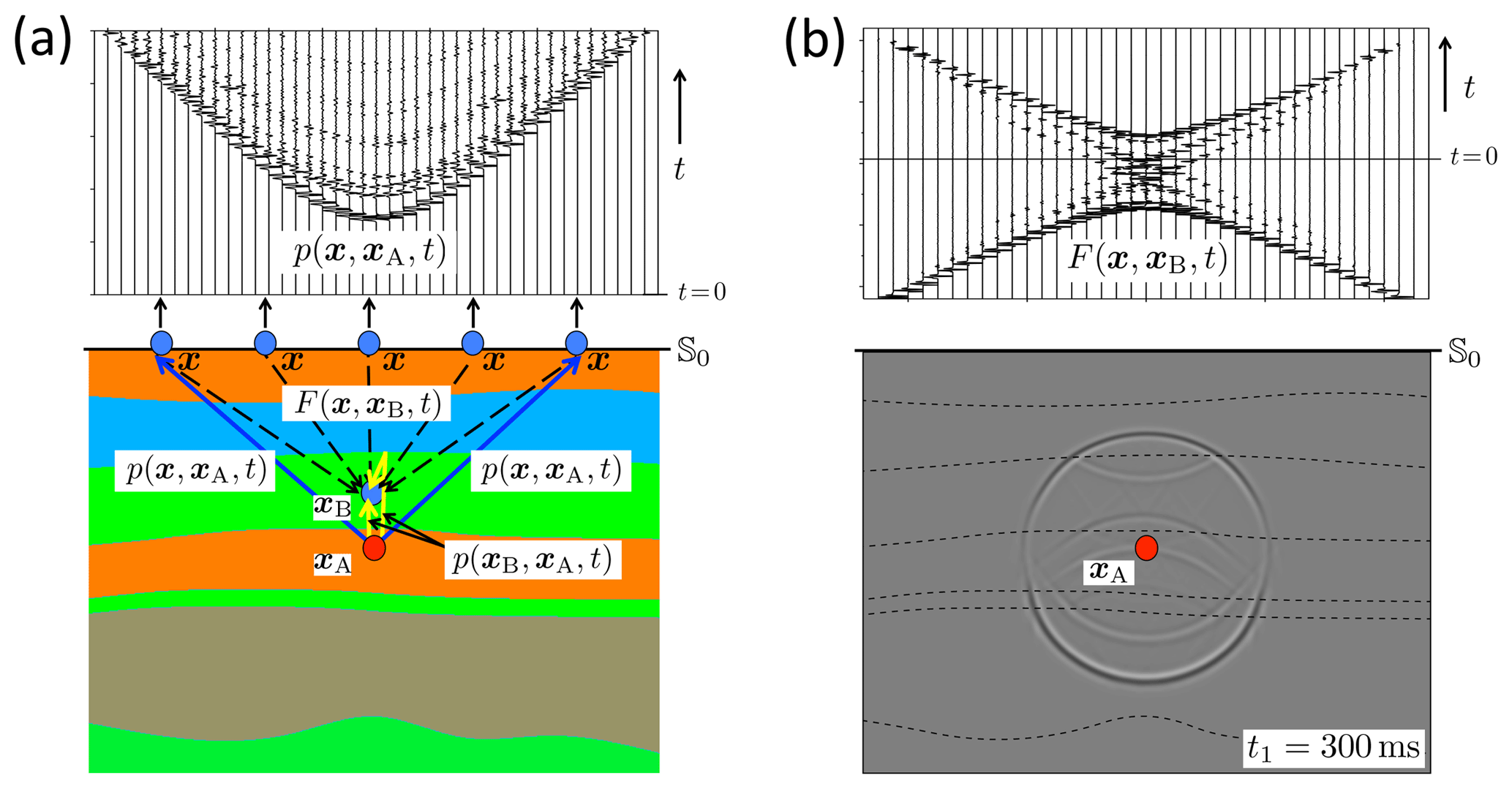
Figure 11 Principle of modified back propagation. (a) The wave field $p(\mathit{x},{\mathit{x}}_{\mathrm{A}},t)$ at the surface 𝕊₀ and illustration of its back propagation to x_B inside the medium. (b) The back propagation operator $F(\mathit{x},{\mathit{x}}_{\mathrm{B}},t)$ (for variable x along 𝕊₀ and fixed x_B) and a snapshot of the back propagated wave field $p({\mathit{x}}_{\mathrm{B}},{\mathit{x}}_{\mathrm{A}},t)$ at t₁=300 ms for all x_B.

This back propagation method has an interesting application in the monitoring of induced seismicity. Assuming $p(\mathit{x},{\mathit{x}}_{\mathrm{A}},t)$ stands for the response to an induced seismic source at x_A, this method creates, in a data-driven way, omnidirectional virtual receivers at any x_B to monitor the emitted field from the source to the surface. This application is extensively discussed in the companion paper (Brackenhoff et al., 2019).

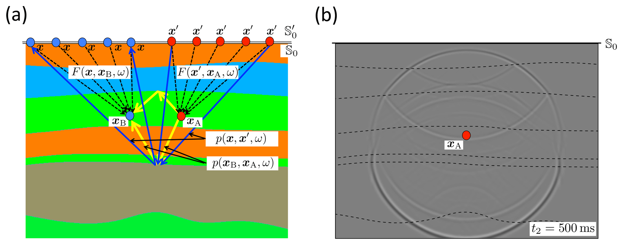
Figure 12 (a) Principle of modified source–receiver redatuming. (b) Snapshot of the wave field $p({\mathit{x}}_{\mathrm{B}},{\mathit{x}}_{\mathrm{A}},t)$ at t₂=500 ms for all x_B.

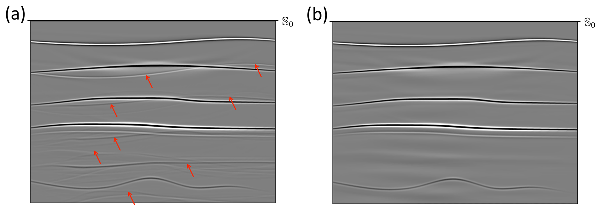
Figure 13 Reflectivity images obtained using the double-focusing method. (a) Classical approach. (b) Modified approach.

3.4 Modified source–receiver redatuming

We modify the approach for source–receiver redatuming. First, in Eq. (39), we replace 𝕊₀ with ${\mathbb{S}}_{\mathrm{0}}^{\prime }$ (just above 𝕊₀), x with ${\mathit{x}}^{\prime }\in {\mathbb{S}}_{\mathrm{0}}^{\prime }$, x_A with x∈𝕊₀ and x_B with x_A. Next, we apply source–receiver reciprocity on both sides of the equation. This yields

$$\begin{array}{ll}{\displaystyle }p(\mathit{x},{\mathit{x}}_{\mathrm{A}},\mathit{\omega })& {\displaystyle }+p^{*}(\mathit{x},{\mathit{x}}_{\mathrm{A}},\mathit{\omega })\\ \text{(41)}& {\displaystyle }& {\displaystyle }=\mathrm{2}\mathrm{\Re }\underset{{\mathbb{S}}_{\mathrm{0}}^{\prime }}{\int }p(\mathit{x},{\mathit{x}}^{\prime },\mathit{\omega })F({\mathit{x}}^{\prime },{\mathit{x}}_{\mathrm{A}},\mathit{\omega })\mathrm{d}{\mathit{x}}^{\prime };\end{array}$$

$F({\mathit{x}}^{\prime },{\mathit{x}}_{\mathrm{A}},\mathit{\omega })$ is defined as in Eq. (40), with ∂₃ replaced by ${\partial }_{\mathrm{3}}^{\prime }$, similar to Eq. (26). The field $p(\mathit{x},{\mathit{x}}^{\prime },\mathit{\omega })=G(\mathit{x},{\mathit{x}}^{\prime },\mathit{\omega })s\left(\mathit{\omega }\right)$ represents the data at the surface. Equation (41) back propagates the sources from x^′ on ${\mathbb{S}}_{\mathrm{0}}^{\prime }$ to x_A. Source–receiver redatuming is now defined as the following two-step process. In step one, apply Eq. (41) to create an omnidirectional virtual source at any desired position x_A in the subsurface. According to the left-hand side, the response to this virtual source is observed by actual receivers at x at the surface. Isolate $p(\mathit{x},{\mathit{x}}_{\mathrm{A}},\mathit{\omega })$ from the left-hand side by applying a time window (a simple Heaviside function) in the time domain. In step two, substitute the retrieved response $p(\mathit{x},{\mathit{x}}_{\mathrm{A}},\mathit{\omega })$ into Eq. (39) to create virtual receivers at any position x_B in the subsurface. Figure 12a illustrates the principle. The operators can be obtained using the Marchenko method. Figure 12b shows a snapshot of $p({\mathit{x}}_{\mathrm{B}},{\mathit{x}}_{\mathrm{A}},t)$ at a time instant $t_{\mathrm{2}}>t_{\mathrm{1}}>\mathrm{0}$ for all x_B (the retrieved snapshot at t₁ is indistinguishable from that in Fig. 11b, which is why we chose to show a snapshot at another time instant). The dashed lines in the snapshot in Fig. 12b indicate the interfaces to aid with the interpretation of the snapshot, but the interfaces need not to be known to obtain this result. This method has an interesting application in forecasting the effects of induced seismicity. Assuming x_A is the position where induced seismicity is likely to take place, this method forecasts the response by creating, in a data-driven way, a virtual source at x_A and virtual receivers at any x_B that observe the propagation and scattering of its emitted field from the source to the surface. This method is extensively discussed in the companion paper (Brackenhoff et al., 2019).

3.5 Modified imaging by double focusing

If we applied imaging to the retrieved response $p({\mathit{x}}_{\mathrm{B}},{\mathit{x}}_{\mathrm{A}},\mathit{\omega })+p^{*}({\mathit{x}}_{\mathrm{B}},{\mathit{x}}_{\mathrm{A}},\mathit{\omega })$ in a similar fashion to Eq. (29), we would obtain an image of the virtual sources instead of the reflectivity. Similar to Sect. 2.5 we need a process to obtain the decomposed response $p^{-,+}({\mathit{x}}_{\mathrm{B}},{\mathit{x}}_{\mathrm{A}},\mathit{\omega })$. Our starting point is Eq. (34), in which we interchange x_A and x_B and choose both of these points at 𝕊_A, such that $f_{\mathrm{1}}^{-}({\mathit{x}}_{\mathrm{A}},{\mathit{x}}_{\mathrm{B}},\mathit{\omega })=\mathrm{0}$. Applying source–receiver reciprocity on the left-hand side and multiplying both sides by a source spectrum s(ω), we obtain

$$\begin{array}{}\text{(42)}& p^{-,+}({\mathit{x}}_{\mathrm{B}},{\mathit{x}}_{\mathrm{A}},\mathit{\omega })=\underset{{\mathbb{S}}_{\mathrm{0}}}{\int }{F}^{+}(\mathit{x},{\mathit{x}}_{\mathrm{B}},\mathit{\omega })p^{-,+}(\mathit{x},{\mathit{x}}_{\mathrm{A}},\mathit{\omega })\mathrm{d}\mathit{x},\end{array}$$

with $p^{-,+}(\mathit{x},{\mathit{x}}_{\mathrm{A}},\mathit{\omega })=G^{-,+}(\mathit{x},{\mathit{x}}_{\mathrm{A}},\mathit{\omega })s\left(\mathit{\omega }\right)$ and

$$\begin{array}{}\text{(43)}& F^{+}(\mathit{x},{\mathit{x}}_{\mathrm{B}},\mathit{\omega })={\displaystyle \frac{\mathrm{2}}{i\mathit{\omega }{\mathit{\rho }}_{\mathrm{0}}}}{\partial }_{\mathrm{3}}{f}_{\mathrm{1}}^{+}(\mathit{x},{\mathit{x}}_{\mathrm{B}},\mathit{\omega }).\end{array}$$

Next, in Eq. (34), replace 𝕊₀ with ${\mathbb{S}}_{\mathrm{0}}^{\prime }$ (just above 𝕊₀), x with ${\mathit{x}}^{\prime }\in {\mathbb{S}}_{\mathrm{0}}^{\prime }$ and x_B with x∈𝕊₀. Applying source–receiver reciprocity on the right-hand side and multiplying both sides by a source spectrum s(ω), we obtain

$$\begin{array}{ll}{\displaystyle }{p}^{-,+}(\mathit{x},{\mathit{x}}_{\mathrm{A}},\mathit{\omega })& {\displaystyle }=\underset{{\mathbb{S}}_{\mathrm{0}}^{\prime }}{\int }{p}^{-,+}(\mathit{x},{\mathit{x}}^{\prime },\mathit{\omega })F^{+}({\mathit{x}}^{\prime },{\mathit{x}}_{\mathrm{A}},\mathit{\omega })\mathrm{d}{\mathit{x}}^{\prime }\\ \text{(44)}& {\displaystyle }& {\displaystyle }-f_{\mathrm{1}}^{-}(\mathit{x},{\mathit{x}}_{\mathrm{A}},\mathit{\omega })s\left(\mathit{\omega }\right);\end{array}$$

$F^{+}({\mathit{x}}^{\prime },{\mathit{x}}_{\mathrm{A}},\mathit{\omega })$ is defined as in Eq. (43), with ∂₃ replaced by ${\partial }_{\mathrm{3}}^{\prime }$, similar to Eq. (26). Substitution of Eq. (44) into Eq. (42) yields

$$\begin{array}{ll}{\displaystyle }& {\displaystyle }{p}^{-,+}({\mathit{x}}_{\mathrm{B}},{\mathit{x}}_{\mathrm{A}},\mathit{\omega })+\underset{{\mathbb{S}}_{\mathrm{0}}}{\int }{F}^{+}(\mathit{x},{\mathit{x}}_{\mathrm{B}},\mathit{\omega })f_{\mathrm{1}}^{-}(\mathit{x},{\mathit{x}}_{\mathrm{A}},\mathit{\omega })s\left(\mathit{\omega }\right)\mathrm{d}\mathit{x}\\ \text{(45)}& {\displaystyle }& {\displaystyle }=\underset{{\mathbb{S}}_{\mathrm{0}}}{\int }\underset{{\mathbb{S}}_{\mathrm{0}}^{\prime }}{\int }{F}^{+}(\mathit{x},{\mathit{x}}_{\mathrm{B}},\mathit{\omega })p^{-,+}(\mathit{x},{\mathit{x}}^{\prime },\mathit{\omega })F^{+}({\mathit{x}}^{\prime },{\mathit{x}}_{\mathrm{A}},\mathit{\omega })\mathrm{d}{\mathit{x}}^{\prime }\mathrm{d}\mathit{x}.\end{array}$$

This is the modified version of Eq. (28), with the operators $F_{\mathrm{d}}^{+}$, which account for primaries only, replaced by the operators F⁺, which account for both primaries and multiples. These operators can be obtained using the Marchenko method from the reflection data $p^{-,+}(\mathit{x},{\mathit{x}}^{\prime },\mathit{\omega })$ and a smooth model of the medium to define the initial estimate of $f_{\mathrm{1}}^{+}$. The second term on the left-hand side can be removed by a time-window in the time domain, which leaves the redatumed reflection response $p^{-,+}({\mathit{x}}_{\mathrm{B}},{\mathit{x}}_{\mathrm{A}},\mathit{\omega })$. The reflectivity imaging step to retrieve r(x_A) is the same as that in Eq. (29) and is not repeated here. Figure 13b shows an image obtained by applying Eqs. (45) and (29) for all x_A in the region of interest, for the same medium that was imaged using the classical double-focusing method (which for ease of comparison is repeated in Fig. 13a). Note that the artefacts caused by the internal multiple reflections (indicated by the red arrows in Fig. 13a), have almost entirely been removed. In practical situations the modified method may suffer from imperfections in the data, such as incomplete sampling, anelastic losses, out-of-plane reflections and 3-D spreading effects. Several of these imperfections can be accounted for by making the method adaptive (van der Neut et al., 2014). Promising results have been obtained using real data (Ravasi et al., 2016; Staring et al., 2018).

Other methods exist that deal with internal multiple reflections in imaging. Davydenko and Verschuur (2017) discuss a method called full wave field migration. This is a recursive method, starting at the surface, which alternately resolves layer interfaces and predicts the multiples related to these interfaces. In contrast, Eq. (45) is non-recursive. The field $p^{-,+}({\mathit{x}}_{\mathrm{B}},{\mathit{x}}_{\mathrm{A}},\mathit{\omega })$ at 𝕊_A is obtained without needing information about the layer interfaces between 𝕊₀ and 𝕊_A; a smooth model suffices. Following the work of Weglein et al. (1997, 2011) on an inverse-scattering series approach to multiple elimination, Ten Kroode (2002) proposes a method that attenuates the internal multiples directly in the reflection data at the surface, without requiring model information. This method resembles a multiple prediction and removal method proposed by Jakubowicz (1998). These methods address all orders of internal multiples, but only with approximate amplitudes. Variants of the Marchenko method have been developed that aim to eliminate the internal multiples from the reflection data at the surface (Meles et al., 2015; van der Neut and Wapenaar, 2016; Zhang et al., 2019). The last reference shows that all orders of multiples are, at least in theory, predicted with the correct amplitudes without needing model information. Once the internal multiples have been successfully eliminated from the reflection data at the surface, standard redatuming and imaging (for example as described in Sect. 2.5) can be used to form an accurate image of the subsurface, without artefacts caused by multiple reflections.

4 Conclusions

The classical homogeneous Green's function representation, originally developed for optical image formation by holograms, expresses the Green's function plus its time-reversal between two arbitrary points in terms of an integral along a surface enclosing these points. It forms a unified basis for a variety of seismic imaging methods, such as time-reversal acoustics, seismic interferometry, back propagation, source–receiver redatuming and imaging by double focusing. We have derived each of these methods by applying some simple manipulations to the classical homogeneous Green's function representation, which implies that these methods are all very similar. As a consequence, they share the same advantages and limitations. Because the underlying representation is exact, it accounts for all orders of multiple scattering. This property is exploited by seismic interferometry in a layered medium below a free surface and, to some extent, by time-reversal acoustics in a medium with random scatterers. However, in most cases multiple scattering is not correctly handled because in practical situations data are not available on a closed surface. We also discussed a single-sided homogeneous Green's function representation, which requires access to the medium from one side only, say from the Earth's surface. This single-sided representation ignores evanescent waves, but it accounts for all orders of multiple scattering, similar as the classical closed-surface representation. We used the single-sided representation as the basis for deriving modifications of time-reversal acoustics, back propagation, source–receiver redatuming and imaging by double focusing. These methods account for multiple scattering and can be used to obtain accurate images of the source or the subsurface, without artefacts related to multiple scattering. Another interesting application is the monitoring and forecasting of responses to induced seismic sources, which is discussed in detail in a companion paper.