the Creative Commons Attribution 4.0 License.
the Creative Commons Attribution 4.0 License.
 | 04 Sep 2020
Data acquisition by digitizing 2-D fracture networks and topographic lineaments in geographic information systems: further development and applications
Romesh Palamakumbura
Maarten Krabbendam
Katie Whitbread
Christian Arnhardt
Understanding the impact of fracture networks on rock mass properties is an essential part of a wide range of applications in geosciences from understanding permeability of groundwater aquifers and hydrocarbon reservoirs to erodibility properties and slope stability of rock masses for geotechnical engineering. However, gathering high-quality, oriented-fracture datasets in the field can be difficult and time-consuming, for example, due to constraints on field work time or access (e.g. cliffs). Therefore, a method for obtaining accurate, quantitative fracture data from photographs is a significant benefit. In this paper we describe a method for generating a series of digital fracture traces in a geographic information system (GIS) environment, in which spatial analysis of a fracture network can be carried out. The method is not meant to replace the gathering of data in the field but to be used in conjunction with it, and it is well suited when field work time is limited or when the section cannot be accessed directly. The basis of the method is the generation of the vector dataset (shapefile) of a fracture network from a georeferenced photograph of an outcrop in a GIS environment. From that shapefile, key parameters such as fracture density and orientation can be calculated. Furthermore, in the GIS environment more complex spatial calculations and graphical plots can be carried out such as heat maps of fracture density. Advantages and limitations compared to other fracture network capture methods are discussed.
- Article
(21674 KB) - Full-text XML
-
Supplement
(110 KB) - BibTeX
- EndNote


Fractures are the main pathways of fluid flow in rocks, and they exert a strong influence on rock mass properties. The characterization of fracture networks is an essential aspect of various applications in the earth sciences, such as understanding the behaviour of fluid flow in groundwater aquifers (Singhal and Gupta, 2010) and hydrocarbon reservoirs and the erodibility and slope stability of rock masses (Clarke and Burbank, 2010; Krabbendam and Glasser, 2011). Fracture network data are essential for assessing future sites of nuclear waste repositories (Follin et al., 2014), predicting rock slope stability (Selby, 1982; Park et al., 2005) and understanding rock mass strength for the engineering of infrastructure (Hoek and Brown, 1997; Zhan et al., 2017; Ren et al., 2017). Thus, fracture network analysis is a critical component of applied geological characterization required for ensuring water and energy security, supporting infrastructure development, and protecting human health, which are identified as key Sustainable Development Goals (Schrodt et al., 2019).
To characterize fracture networks, a range of fracture network parameters need to be acquired, including the fracture density, connectivity and orientations (e.g. Singhal and Gupta, 2010). These properties can be highly spatially variable over a range of scales which cannot be accurately predicted (Long and Billaux, 1987). The comprehensive capture of observational data is typically required to characterize fracture network variability over large areas. Due to the limited distribution of suitable rock exposures in many settings, understanding the spatial variability of fracture network parameters at regional scales requires sampling at multiple sites (e.g. McCaffrey et al., 2020). Practical constraints on data collection are therefore critical factors. Constraints on the number of sites that can be analysed in a given study increase uncertainty in estimations of fracture properties of the wider rock mass. This uncertainty limits the scales at which analyses can be reasonably applied.
The need for efficient and robust methods for quantitative capture of fracture data is well recognized, and methods using statistically based observational techniques (Mauldon et al., 2001) and systematic regional sampling (e.g. Watkins et al., 2015a) have been proposed previously. We build on previous developments in fracture sampling by focusing on a method for digital data capture from 2-D outcrop images.
Advanced 3-D methods for outcrop imaging and fracture analysis are now available (Tavani et al., 2016; Bisdom et al., 2017), but limited access to necessary hardware, software and training technology may limit the wider adoption of these high-cost techniques in many applied research contexts. In contrast, the ready availability of digital cameras and suitable open-source software means that the 2-D digital capture method has potential for wider adoption across applied geoscience fields in which traditional, low-cost 1-D and analogue sampling methods are still widely used (Siddique et al., 2015; Panthee et al., 2016). Systematic 2-D digital capture has a particular relevance for studies in which (1) large datasets are required from multiple sites, (2) advanced outcrop scanning or unmanned aerial vehicle (UAV) systems are not available or are impractical to use, (3) historic images (such as from quarries, canal excavations or road cuttings) provide a valuable data source, and (4) multi-scalar analyses are performed using micro-scale (e.g. thin section) to macro-scale (e.g. satellite) images.
Here we describe good practice in the use of a low-cost 2-D digital method for the efficient capture and visualization of a range of fracture parameters and illustrate how these methods can be used across a range of applied geoscience fields (Fig. 1). Although the method has been used before (Krabbendam and Bradwell, 2014; Watkins et al., 2015a; Krabbendam et al., 2016; Healy et al., 2017), no comprehensive description of the method has been published.
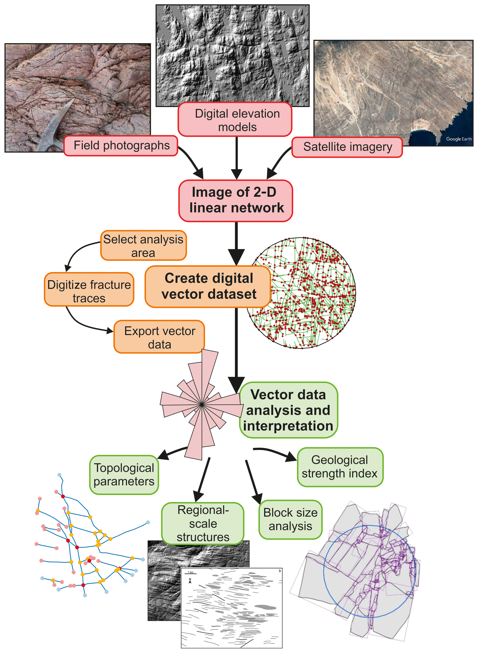
Figure 1Flowchart providing an overview of the 2-D digital capture method used for digitizing linear features, from preparing an image and digitizing the features to the output of data. Digital elevation model examples are taken from NEXTMap© in Scotland, and the example of the satellite image of Oman is taken from Google Earth©.
Understanding the effect of a fracture network on the properties of a rock mass requires the acquisition of various parameters such as length, orientations, density and spacing (Singhal and Gupta, 2010). Network topology is used to understand how connected a fracture network is and can be characterized by derived parameters such as fracture connectivity, percolation potential and clustering (Manzocchi, 2002; Sanderson and Nixon, 2015). Finally, fracture aperture, fill and paragenesis history provide an important understanding of the fracture network history, fluid flow and fracture strength (Carlsson and Olsson, 1976; Laubach et al., 2019).
Fracture networks can be characterized in different dimensions using a number of approaches. 1-D approaches include outcrop-based scanline surveys and (by necessity) borehole fracture analysis, typically represented by the number of fractures per unit length, i.e. frequency. 1-D approaches are relatively rapid but do not directly constrain parameters such as fracture length and connectivity. If the fracture network is anisotropic, which is commonly the case, the characterization is biased by the orientation of the scanline or the borehole (orientation bias; Singhal and Gupta, 2010; Zeeb et al., 2013; Watkins et al., 2015b).
In 2-D fracture network analysis, a circular sampling window is commonly used (Davies et al., 2011; Rohrbaugh et al., 2002; Watkins et al., 2015a). In the field, a circular chalk line is drawn on an outcrop, within which the fractures and key geometries are captured. Connectivity within the fracture network can be parameterized by characterizing the different types of fracture terminations and intersections, which can be used to understand fluid percolation potential (e.g. Manzocchi, 2002). Full field-based capture is very time-consuming, particularly when data from multiple sites are required, and may be impractical or impossible for some outcrops such as quarries, cliffs and coastal platforms. Time constraints normally mean that field-based methods are also limited in their scale of application, with sampling window diameters of 1–2 m being commonly used (e.g. Watkins et al., 2015a; Procter and Sanderson, 2018). This limitation means that spatial variability in fracture properties at scales greater than 5–10 m are typically not captured.
To overcome the time constraints of the full 2-D window approach, a circular scanline method was developed (Mauldon et al., 2001) in which only those fractures that intersect a particular circular scanline are captured; in a sense it is similar to the 1-D approach. The circular scanline analysis is more rapid than the full 2-D circular window analysis and has less length and orientation bias compared to 1-D methods (Mauldon et al., 2001). The circular scanline method can be used to calculate proxies for (but does not directly measure) fracture density and length based on the ratio of the types of trace intersections (Mauldon et al., 2001); however, if other parameters are needed, further field work would be required.
Ideally, for any application, a full 3-D characterization of the rock mass would be achieved. However, the true 3-D characterization of a rock mass is currently only possible using CT scanning and is restricted to very small samples (Voorn et al., 2015). High-resolution 3-D images of outcrop surfaces (more like 2.5-D) can be captured by laser scanning, which can be ground based or acquired by UAV (e.g. Bisdom et al., 2017; Gao et al., 2017; Wüstefeld et al., 2018). From the laser scans, 3-D images of the outcrop surface (3-D virtual outcrop) can be generated using techniques such as structure from motion (SfM) photogrammetry (Vasuki et al., 2014). These can provide additional information on fracture orientation through the use of advanced image analysis techniques (Wüstefeld et al., 2018). These methods have been used for advanced fracture network analysis and modelling for applications related to fluid flow, gas migration and engineering/construction (e.g. Bisdom et al., 2017; Menegoni et al., 2019; Strijker et al., 2012; Tavani et al., 2016). These 3-D scanning techniques require sophisticated hardware, proprietary software and training that potentially limits their applicability. In addition, there are practical limitations at sites, such as access and restrictions on the use of UAVs, that may further limit their use (e.g. Senger et al., 2015).
The 2-D fracture network can be captured in the field, as well as from image tracing (e.g. Watkins et al., 2015a). Digital 2-D data capture can be applied to photographs of an outcrop or thin section, aerial photographs, or satellite imagery. Digital 2-D data capture methods can thus be used at a great range of scales, permit data acquisition from inaccessible sites and provide a reproducible approach from which a digital dataset suitable for numerical and statistical analysis can be readily derived. The 2-D digital capture typically relies on geographic-information-system-type (GIS) functions for the visualization and analysis of images and uses standard GIS tools. More sophisticated analysis can be carried out using software applications such as the proprietary DigiFract which is based on customized quantum GIS (QGIS) functions (Hardebol and Bertotti, 2013), the open-source tool FracPaQ for MATLAB (Healy et al., 2017) and NetworkGT for QGIS (Nyberg et al., 2018). These tools provide enhanced functions for the efficient capture of data from images and advance data analysis but are targeted for applications in structural geology research contexts.
In its basic form, the 2-D digital data capture method requires only a digital camera, a measuring stick and access to GIS such as open-source QGIS. The low-cost nature of the method means that this is potentially a powerful tool for enhancing geological investigations across a range of applied studies such as engineering geology and hydrogeology. We comprehensively describe good practice for 2-D digital fracture capture and analysis. In particular, we focus on the practical aspects of image capture, preparation and analysis using QGIS and other open-source tools and plugins. Four case studies are presented to illustrate a number of practical applications. We demonstrate some simple fracture analysis tools that can be applied to the captured data. Finally, we evaluate the benefits and drawbacks of 2-D digital data capture compared to other approaches for capturing fracture data.
The 2-D digital capture method in essence captures a set of digital traces (vectors) of a 2-D linear feature network in a GIS project from a georeferenced image. Here, we use open-source GIS software (QGIS), making the method accessible to all potential users. A number of open tools within QGIS can be used for a more advanced analysis of the digitized fracture network.
3.1 Outcrop selection
A suitable outcrop for digital fracture analysis must be first selected. The outcrops selected will depend on the nature of the study being undertaken and the type of fracture network parameters required (Watkins et al., 2015a). It is important to consider whether the outcrop is representative of the rock mass as a whole or whether multiple sites would better represent the diversity of fracture characteristics. Outcrop selection has significant implications on the final results, i.e. if the outcrop is a proxy for wider-scale fracture network characteristics at depth or if it is the outcrop itself that is being studied in isolation (Laubach et al., 2019; Ukar et al., 2019).
3.2 Outcrop image preparation
The first step is to capture or prepare a suitable photograph or image of the outcrop to be analysed. The image can be a photograph of a fracture network of outcrops of various scales from centimetres to tens of metres. It is important that the fractures can be clearly identified in the photograph and that not too much of the image is occupied by vegetation or broken ground (Fig. 2a). It is important to include an accurate and clearly identifiable scale; a strip of plywood with duct tape works very well. However, in some dangerous outcrops (e.g. working quarries) this may be impractical and quarry machinery or other features of known dimensions may be used as a scale in the photograph. This also applies to historic photographs. The photograph should be taken at right angles (or as much as possible) to the outcrop to minimize the issues created by a distortion of the image. The camera should have a focal length of 35 mm (analogue 35 mm equivalent) or longer to prevent further distortion. Horizontal outcrops should be photographed vertically to again minimize the distortion of the fractures. Mounting the camera on a stick is useful to increase the distance and capture a larger field of view (Fig. 2b, c); drones can also be used. For horizontal outcrops, it is convenient to orient the measuring stick accurately to the north using a compass (Fig. 2c), which will help in capturing the correct orientations of the fractures.
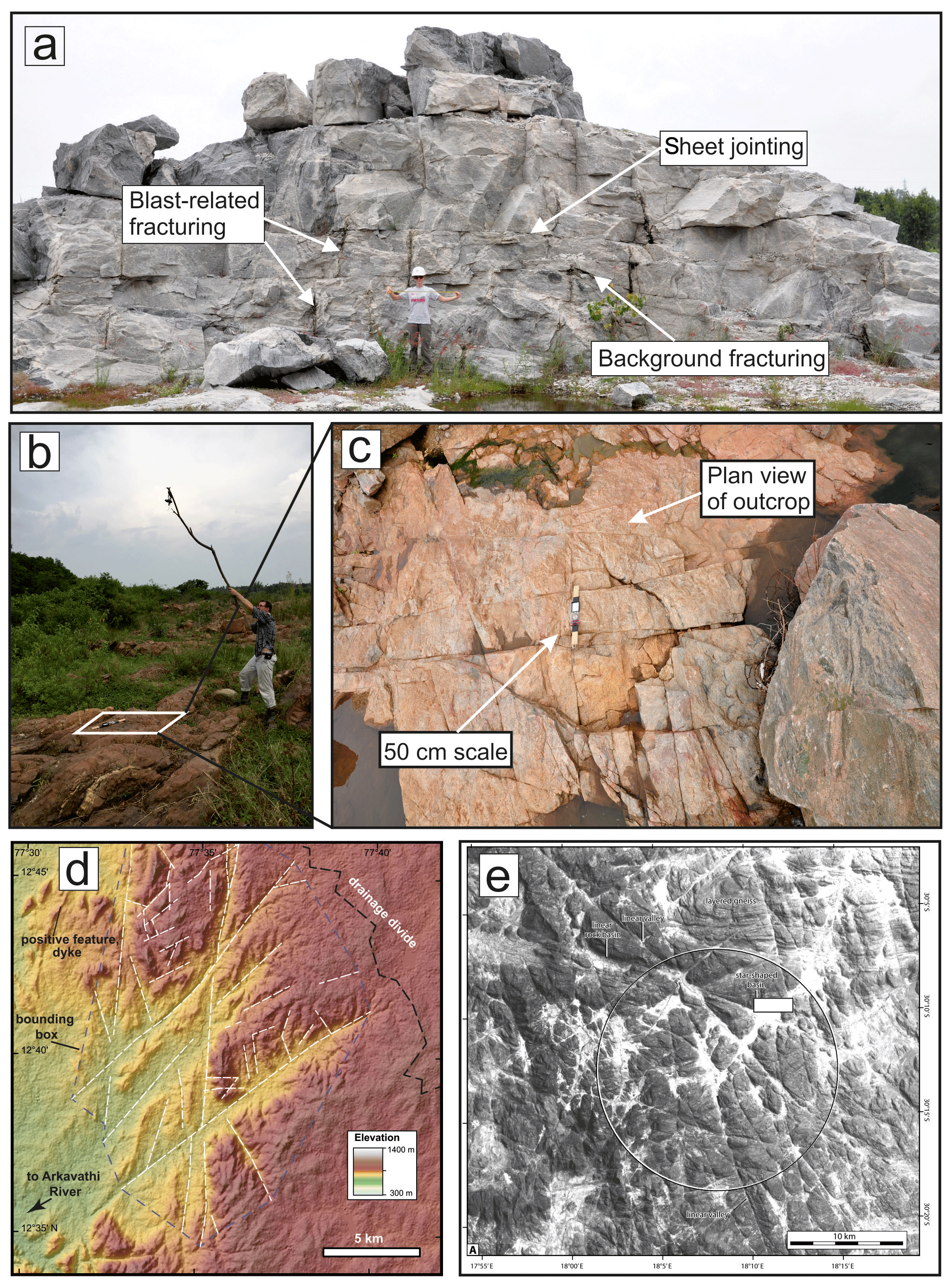
Figure 2Examples of photographs and digital elevation model (DEM) images that can be used for digitizing 2-D linear features, including (a–c) photographs of fracture networks of various scales from southern India and improvised methods for taking photographs parallel to the outcrop, (d) a DEM image from southern India of larger kilometre-scale features that could also be digitized, and (e) an aerial photograph from Namibia (adapted from Krabbendam and Bradwell, 2014).
3.3 Georeferencing the images
To aid robust georeferencing, the photograph needs to have a square of known size (e.g. 1 m×1 m) embedded in it. This is done by importing the photograph into a graphics software package (such as Inkscape) and drawing a square based on the scale included in the original photograph (Fig. 3). The photograph with the embedded 1 m×1 m square is then imported into a new GIS project file. The GIS project file needs a projection in metres; we recommend a Mercator projection (such as EPSG:3857). Within the GIS project, a vector grid (fishnet grid) is created with a grid extent that is larger than the imported photograph and with a vertical and horizontal spacing of 1.0 m. Finally, the square on the photograph is georeferenced to a square on the fishnet grid (Fig. 3a).

Figure 3Images showing (ai–aii) how to georeference an image to a fishnet grid (black) from a square of a known scale (white); and (b) the tools available for digitizing fractures in QGIS, including (i) a fully manual method and (ii) a semi-automatic method such as Geotrace.
3.4 Using DEM, satellite and air photo images
DEMs (digital elevation models) (and their hill-shaded derivatives), satellite images and (orthorectified) aerial photographs commonly show good topographic lineaments that likely represent fracture zones or master joints (Fig. 2d, e). Such imagery is commonly already georeferenced and can be used without further preparation. It should be noted, however, that aerial photographs, DEMs and satellite images do not directly show fracture traces, rather they show the topographic expression of these. Thus, fracture density is likely to be underestimated because fractures without topographic expression will not be captured. Figure 2d is an example of a DEM image from southern India showing kilometre-scale 2-D topographic lineaments; in some parts lineaments are well developed, but in other parts fracture zones have no expression and presumably occur beneath a continuous layer of regolith. Furthermore, such imagery is limited by the on-the-ground resolution so that smaller-scale (smaller aperture) fractures may not appear. Hill-shade DEM images, as well as satellite imagery and aerial photographs, have the problem of bias by a particular direction of illumination so that lineaments of one orientation may be clearer than others. For DEMs, hill-shade derivatives with different illumination direction can be made; for satellite imagery, sometimes images taken at a different time of day are available. Hence, for DEM-scale interpretations it is important to take a multi-data-type approach (e.g. DEMs and satellite images) to guide digitization, similar to that of Pless (2012).
3.5 Data capture
3.5.1 Create analysis window
As a first step, create a polygon shapefile and digitize the area (window) to be analysed. An example is shown in Fig. 3b as two circular windows (in white) are digitized onto a photograph in GIS. It is important to create a different ID number for each shape that includes details of the photograph or image that is being digitized. Multiple windows can be used on the same image, in particular if the image shows spatial variability of the fracture network.
3.5.2 Digitize linear features
This step aims to create a series of digital line traces from the georeferenced image. Create a new line shapefile in the GIS project to hold the linear trace data. The shapefile needs to include an ID column in the attribute table so that the linear traces can be associated with their specific window polygon. Two methods can be used to create digital traces of the linear features. Firstly, the individual features can be digitized manually in the GIS project using the “add line features” tool. Alternatively, the plugin tool Geotrace can be used to semi-automate the digitizing process. The Geotrace plugin tool in QGIS allows one to click on the start and end of each fracture, and Geotrace creates a line vector between these points. For this method, the photograph must be in greyscale because the plugin follows the linear feature based on low raster values and requires a sharp contrast between the feature and the background. When digitizing fracture traces, it is important to only digitize in one orientation; if a feature has multiple orientations along its length, then multiple line segments should be digitized. Figure 3b is an example of both (i) manual digitization and (ii) semi-automated digitization with Geotrace. In both the manual and semi-automated methods, connecting fractures should be properly snapped to each other and to the surrounding circular window.
In quarries or excavated sections, it can be challenging to distinguish natural joints from those arising from quarrying processes such as blast damage or drilling related fractures. Using field observations, blast damage can be separated from natural joints (Fig. 2a). Joints arising from blast damage can easily be distinguished from natural joints as they do not fit with the overall fracture pattern and are generally surrounded by small radiating fractures.
3.6 Data output and further analysis
The final step is to generate basic parameters and calculate dimensions from the digital traces of the linear features. There are a number of different ways that the vector data can be processed, which include the following: (1) using the field calculator in QGIS, (2) as an exported spreadsheet or (3) using a programming language such as Python or R to make calculations from the spreadsheet or directly from the shapefile.
Primary parameters such as length and orientation of individual fracture traces can be calculated within the field calculator in the QGIS attribute table. The area of the circular window can also be calculated in the attribute table using the field calculator. For further processing, the attribute table containing the primary fracture data (length, orientation and reference to the circular window) needs to be exported as a spreadsheet, e.g. in CSV format. Fracture density (D) within the circular window can now be calculated using total length of fractures (ΣL) within the area of the circular window (A), following Singhal and Gupta (2010):
Fracture spacing (S) can be easily derived as this is the reciprocal of fracture density, and it is given by the following (Singhal and Gupta, 1999):
Fracture intersections (points) within the fracture network, important for constraining connectivity (Manzocchi, 2002), can be created as a separate point shapefile with the “line intersection” tool. The digitized fracture traces can also be used to derive block size parameters using the “polygonize” tool to convert the line vectors into polygons. As before, parameters such as area can be derived using the field calculator in the attribute table and exporting as a spreadsheet.
To illustrate the use of systematic 2-D digital fracture analysis methods for applied geoscience investigation, we present a number of case studies to highlight a range of geoscience applications and illustrate key benefits, including (1) rapid data collection to support regional hydrogeological assessment (India), (2) enabling the quantitative, rather than typical qualitative, assessment of key parameters for engineering rock mass strength evaluation (India), (3) analysing catchment-scale variability in sediment source characteristics for applied geomorphic studies in erosional terrains (Scotland), and (4) fracture network analysis from historical images for sites where modern exposures are unavailable (Sweden).
4.1 Understanding fracture connectivity and permeability, southern India
Characterization of fracture networks is essential to understand local- and regional-scale aquifer properties such as connectivity and permeability, in particular in fractured hard-rock aquifers in which fractures are the primary water stores and pathways (e.g. Stober and Bucher, 2007; Singhal and Gupta, 2010; Guihéneuf et al., 2014). An example is given here of the Peninsular Gneiss in the Cauvery Catchment in southern India. The groundwater properties of the Cauvery Catchment have been an area of ongoing research (Maréchal et al., 2006; Perrin et al., 2011; Collins et al., 2020) as the spatial and temporal variability of groundwater availability has profound implications for the sustainability of irrigation and hence food security. Two contrasting basement fracture networks can be identified (Fig. 4a–b): firstly, a massive gneiss with few fractures dominated by a widely spaced background jointing and sheeting joints close to the surface; and secondly, fracture zones that are characterized by a very dense fracture network. Data were collected during a very short reconnaissance-type field work trip.
Length-weighted rose plots show the variation in orientation of fractures (in a vertical section) in the two identified domains (Fig. 4c, d). In the massive gneiss, the fractures are generally orientated sub-horizontally with several short connecting vertical fractures. In contrast, fractures in the fracture zones are generally orientated sub-vertically with short connecting sub-horizontal fractures. The fracture density in the fracture zones is an order of magnitude higher than in the massive gneiss (Table 1). Using NetworkGT (Nyberg et al., 2018), the fracture branches and nodes (intersections and fracture trace end points) were characterized based on the topology of the branch intersections (Manzocchi, 2002; Sanderson and Nixon, 2015). The massive gneiss is dominated by I-type nodes, whereas the fracture zones predominantly contain a combination of Y and X type nodes (Fig. 4a–b; for node types see Fig. 4g) (Table 1). Heat maps of intersection clustering illustrate the higher fracture connectivity within the fracture zones. To quantify the connectivity, the connections per line and dimensionless intensity (a representation of intensity that uses average fracture length) were calculated (following Sanderson and Nixon, 2015) (Table 1; Fig. 4h). The number of connected (X and Y) nodes per fracture line length is an indication of the percolation potential of a fracture network (Sanderson and Nixon, 2018). The fracture zones have the highest connections per line length and dimensionless intensity, indicating they have the highest potential connectivity. In contrast, the background gneiss has the lowest connections per line and intensity, suggesting a relatively low potential connectivity. The coefficient of variation (Cv) was calculated by dividing the standard deviation of the fracture spacing by the mean fracture spacing (Gillespie et al., 1999; Watkins et al., 2015b) and was used to quantify how clustered a fracture network was (Table 1) (Odling et al., 1999). The Cv ratios show that the massive gneiss generally has regularly spaced fractures, while the fractures in the fracture zones are highly clustered (Table 1, Fig. 4h).
Table 1Summary fracture network statistics from the Peninsular Gneiss in the Cauvery Catchment, southern India.
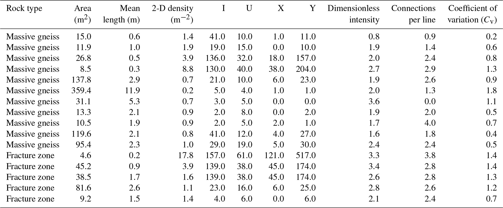
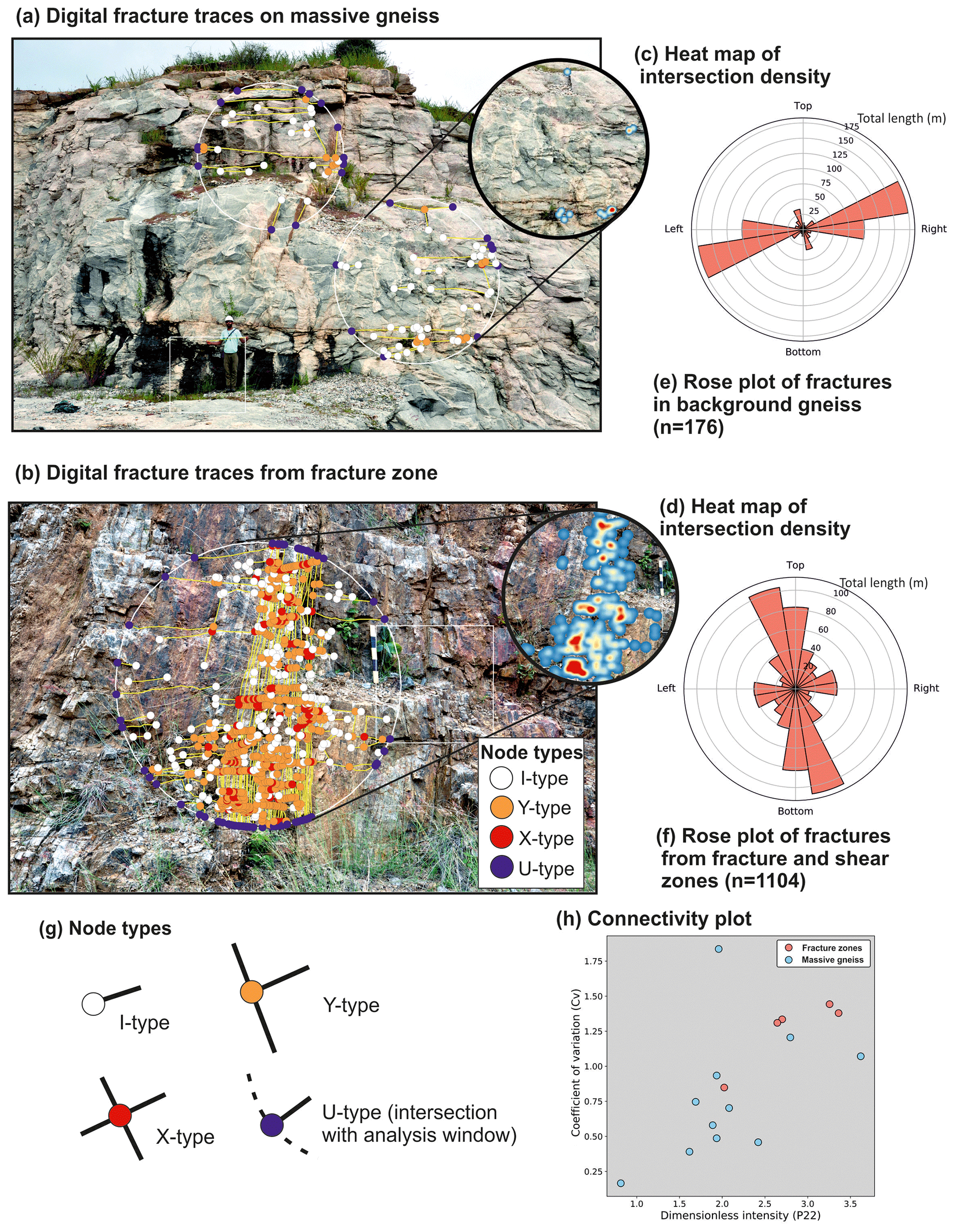
Figure 4Fracture analysis from the Peninsular Gneiss, southern India, including field photographs with digitized fracture branches and intersection types on (a) a massive gneiss example and (b) from a fracture zone; (c–d) heat maps illustrate variations in fracture intersection density (massive gneiss: 0–5 nodes m−2; fracture zones: 0–18 nodes m−2); (e–f) length-weighted rose plots showing the variation in orientation of fracture traces in the background gneiss and fracture zones; (g) a schematic illustration of the various types of fracture connections (as defined by Manzocchi, 2002); (h) a plot of connections per line against dimensionless intensity (defined by Sanderson and Nixon, 2015) to show variations in connectivity.
At the near surface, the Peninsular Gneiss has a bimodal fracture density distribution with fracture zones with high fracture density that make up a relatively small proportion of the bedrock, and the majority of the crystalline basement contains a low-density fracture pattern. Derived connectivity parameters indicate the highest potential permeability is found in the fracture zones, whereas the background gneiss has significantly lower potential permeability.
In this case study, field time was limited, and the 2-D digital method provided a rapid and flexible way of gathering fracture network data. It was possible to carry out a reconnaissance survey covering an area over 30 000 km2 and then retrospectively to select the most suitable sites for fracture analysis. Key fracture parameters such as fracture length, orientation and density, which have an impact on aquifer characteristics such as connectivity and permeability across the Peninsular Gneiss in the Cauvery River catchment, were then calculated and used to constrain local- and regional-scale groundwater models (Collins et al., 2020).
4.2 Rock mass strength estimates (geological strength index)
Structural discontinuities are an important control on the engineering behaviour of a rock mass (Barton et al., 1974; Müller, 1974; Hoek, 1983; Hoek and Brown, 1997). Slopes, foundations and underground excavations in hard rock can be strongly affected by the presence of discontinuities; for example, the intersection of structural features can lead to the falling and sliding of blocks or wedges from the surface.
In the last decade, rock mass classification systems have been applied extensively in engineering design and construction (Liu and Chen, 2007). The geological strength index (GSI) system provides a numerical representation of the overall geotechnical properties of a rock mass, which is estimated using a standard matrix chart and field observations of (a) the blockiness of a rock mass and (b) the surface conditions of any discontinuities. The GSI is based on an assessment of the lithology, structure and condition of discontinuity surfaces in the rock mass, and it is estimated from visual examination of the rock mass exposed in surface excavations such as road cuts, in tunnel faces and in borehole cores (Marinos and Hoek, 2000). Both the blockiness and surface conditions, however, are determined in a qualitative and descriptive manner, which is subjective and dependent on the interpreter. Sönmez and Ulusay (1999, 2002) suggested that the blockiness or structure rating should be quantified by using the volumetric joint (fracture) count (Jv; in m−1). This parameter is defined as the sum of the number of joints per metre for each joint set present (Sönmez and Ulusay, 1999):
where S is the spacing of the joints in a set and n is the number of joint sets. The 2-D fracture digitization method can clearly be applied to determine an accurate representation of Jv from an image.
The procedure for quantifying rock mass strength parameters in jointed rocks is illustrated using massive and fractured gneiss exposures in India (Fig. 4). Using the qualitative method (Hoek, 1983), the massive gneiss with “good” fracture surfaces has a GSI index of 70–85, whereas the fractured gneiss with “fair” fracture surfaces has a GSI index of 30–45. To quantify this, the modified GSI methodology from Sönmez and Ulusay (1999) is used. In this example, the massive gneiss has a horizontal joint spacing of 0.81 m (J1) and a vertical joint spacing of 6.19 m (J2). The fractured gneiss has a horizontal joint spacing of 0.17 m (J1) and a vertical joint spacing of 0.08 m (J2). Applying Eq. (3), this gives a Jv value of 1.4 for the massive gneiss and 17.7 for the fractured gneiss. Based on similar estimates of roughness (5), weathering (3) and infill (6), the fracture surface condition rating (SCR) is 14 in both the massive gneiss and the fracture zones. Finally, the GSI values for the massive gneiss were calculated as c. 76 and as c. 44 for the fractured gneiss, demonstrating a more accurate representation of the rock mass strength differences of the massive and fractured gneiss.
4.3 Block size and rock erodibility, Codleteith Burn catchment, southern Scotland
Geohazards related to active geomorphic processes such as debris flows and landslides affect many upland areas. Pre-existing fractures are a significant factor in the preconditioning of rock masses for erosion at the Earth's surface (e.g. Clarke and Burbank, 2010; Dühnforth et al., 2010; Roy et al., 2016). Areas of intensely fractured rocks are thus more likely to be associated with higher susceptibility to debris flow and landslide hazards. This susceptibility is likely to be driven both by higher volumes of material being produced from hillslopes underlain by highly fractured rocks and by the size distribution of sediment grains entering the geomorphic systems (e.g. Sklar et al., 2017). To understand the controls exerted by the rock mass properties on geomorphic systems, the spatial variability in fracture networks in bedrock needs to be adequately characterized at catchment scales. This characterization is challenging in many upland settings as high spatial variability means that large datasets from multiple sites are required, yet practical difficulties accessing sites are common in steep terrain.
The 2-D fracture digitization method is here used to assess the spatial distribution of block size and fracture density of metasandstone of low metamorphic grade in the Southern Uplands, southern Scotland (Fig. 5). The use of the 2-D digital method allowed for a nested sampling approach to characterize variability across a range of length scales, from metre (Fig. 5c) to decimetre (Fig. 5b) to catchment (Fig. 5a). Block density can be expressed as blocks per square metre, which is easily derived from a polygonized set of fracture traces, and is related to the fracture density (Fig. 5d). Whether this 2-D block size measure is representative of the true 3-D block size depends on the anisotropy of the fracture system and the average block shape. Despite consistent bedrock type (metasandstone) across the study area, fault-related fracturing gives rise to highly variable fracture densities across the study area, and variations in 2-D block size estimates range from <50 to >1000 blocks m−2 (Fig. 5d). These data help to quantify the way in which rock mass parameters such as fracture density influence key geomorphic process elements such as block size. This type of data can be used to inform modelling of erosion and sediment movement within landscapes.
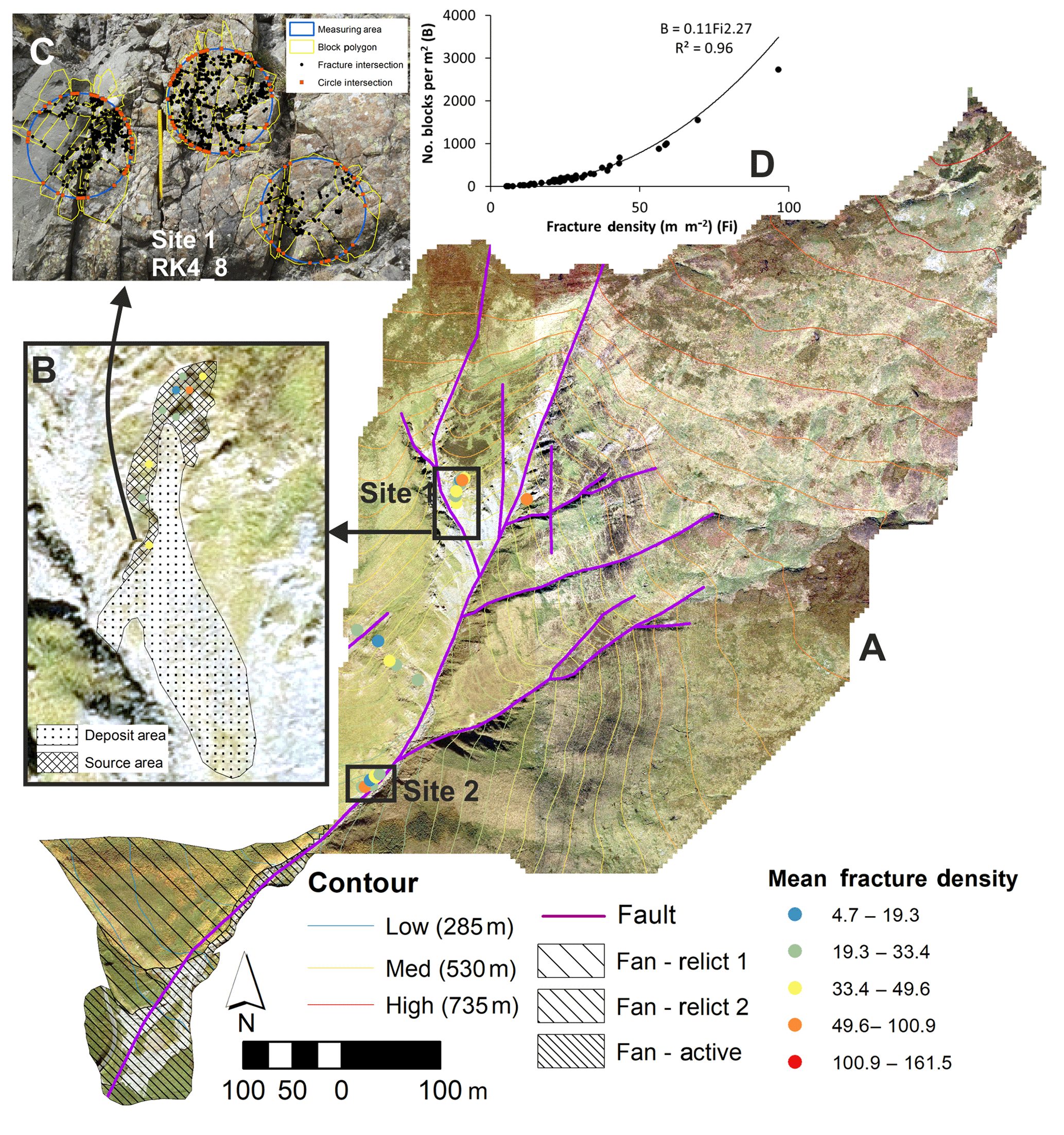
Figure 5Multi-scalar fracture network and block-size analysis for the Codleteith Burn catchment in the Southern Uplands of Scotland (a). Sites 1 (b) and 2 (not shown) are sub-catchment hillslope source areas sampled at high resolution. Variability at the outcrop scale was captured using multiple sampling windows per image (c). The number of blocks sampled per square metre is strongly related to the fracture density (d).
4.4 Application to historic photographs of shallow basement fractures, eastern Sweden
During the construction of the Forsmark nuclear power plant in eastern Sweden in the 1970s, a series of excavations for shafts, tunnels and cooling water canals were dug out in basement gneiss rocks. In these excavations, numerous sub-horizontal fractures were encountered, many of which were dilated and filled with water-lain silt and sand. Many aspects of this shallow fracture network were documented at the time, including aperture and roughness, density, orientation, and coatings (chlorite, epidote, etc.), as well as a characterization of the sediment fills (Stephansson and Ericsson, 1975; Carlsson and Olsson, 1976; Carlsson, 1979). As construction was completed, the excavations were graded, concreted over or filled with water and are not available for study anymore. The shallow fracture network remained of interest in establishing the potential of groundwater overpressure and hydraulic jacking of basement fractures (e.g. Pusch et al., 1990; Talbot, 1990, 2014; Lönnqvist and Hökmark, 2013), as well as playing a potentially important role in a newly recognized erosion mechanism, termed glacial ripping (Hall et al., 2020). For this latter (ongoing) research, one relevant issue is the fracture density of sub-vertical and sub-horizontal fractures as a function of depth in sections with and without fracture dilation; such data were not gathered during the original studies in the 1970s.
To acquire this data, high-quality historic photos were used. All photographs contain a clearly recognizable measuring stick and could thus be georeferenced accurately. Digitization followed the methods described in this paper. Fracture aperture characteristics were attributed to the digital traces based on their appearance in the photographs. The shapefile of fracture traces was imported into python with which spatial parameters such as orientation were calculated and fractures were separated into sub-horizontal and subvertical attitudes. Total fracture trace length was calculated for each 1 m depth interval, and fracture density for each interval was subsequently calculated. The results are plotted as a density–depth profile, and a cubic interpolation was used to smooth the curve (Fig. 6). Results show a clear difference in fracture density between different sections (Fig. 6a, b). A further difference is that in some sections (e.g. SKB-003) both the sub-vertical and subhorizontal fracture densities increase towards rock-head, whilst in other sections (SKB-036) only the sub-horizontal fracture density shows a marked increase.

Figure 62-D fracture analysis applied to historic photographs of excavations during the construction of the Forsmark nuclear power plant, eastern Sweden. Open and tight fractures (red and blue) were digitized. Fracture density was calculated separately for sub-vertical and horizontal fractures. Photos: Göran Hansson, see Carlsson (1979); photos available in the archive of the Swedish Nuclear Fuel and Waste Management Company (SKB).
5.1 Overview of case studies
The case studies presented here highlight a range of benefits from the use of the 2-D digital method for different applications. The Cauvery Catchment case study demonstrates how 2-D digital capture provided flexibility to gather data for the estimation of regional aquifer properties on a short reconnaissance-style field campaign, with fracture data collected retrospectively from photographs taken at key localities. The 2-D digital dataset allows for evolved quantitative and graphical data analysis, such as heat maps of fracture intersections, to better understand connectivity. For engineering geology purposes, commonly used qualitative approaches for estimating key rock mass strength parameters such as the GSI are subject to variability through interpretation bias and practitioner experience, resulting in increased uncertainty and potentially in higher project risks and costs. In the case study presented here, the 2-D digital method is shown to provide a more accurate and consistent representation of the GSI of a rock mass than the commonly used qualitative estimators (e.g. Hoek, 1983; Sönmez and Ulusay, 1999). In geomorphic studies, the quantitative characterization of rock mass strength is increasingly important for the parameterization of process and landscape-evolution models (e.g. Roy et al., 2016; Sklar et al., 2017). The Codleteith Burn (Southern Uplands, Scotland) catchment study demonstrates the potential of the 2-D digital method for multi-scalar fracture analysis in challenging terrain. In eastern Sweden, the historic photographs were the best source for capturing specific fracture parameters in the shallow basement, and the 2-D digital method is the only possible way to retrospectively gather these data.
A number of modern applied geoscience studies, such as in groundwater modelling (Babadagli, 2001), geothermal energy (Hitchmough et al., 2007) and geotechnical engineering (Bandpey et al., 2019), use only field-based methods to gather fracture network data. Field measurements of geometry and density of fracture networks are used to understand the mechanical and hydraulic properties of a rock mass (Babadagli, 2001; Maréchal et al., 2004; Siddique et al., 2015). The 2-D digital method described would be ideally suited to such case studies to improve the quality of data collected and allow for more advanced analysis. In these studies, field time and accessibility of the outcrop are a major consideration for the type and amount of fracture data collected. When time is limited, a 1-D method is used to collect fracture data (Bandpey et al., 2017), whereas the new digital method would allow full 2-D fracture traces to be collected efficiently. In studies that look at slope stability on narrow mountain roads in the Himalayas (Siddique et al., 2015), limited fracture data are used in rock-quality calculations, which is likely due to a combination of time constraints and the inaccessibility of the outcrop. The digital method would provide a more accurate estimate of fracture geometries when modelling slope processes (e.g. Pradhan and Siddique, 2020).
5.2 Benefits and limitations
The capture and publication of digital objects such as digital fracture network traces and derived parameters are an increasingly valuable part of the geoscience research process, facilitating the evaluation and support of ongoing scientific discovery (Gil et al., 2016). The case studies demonstrate that the 2-D digital method described herein represents a valuable tool for analysing fracture networks, facilitating the efficient capture of quantitative datasets through a systematic and reproducible approach. Nevertheless, there are benefits and limitations compared to other fracture capture methods.
The 2-D digital method is as rapid, if not more so, than a 1-D scan-line survey. However, the 2-D digital method does not capture the direct field observations such as orientation, roughness, aperture and any secondary fills. These parameters are useful for understanding rock mass strength or permeability (Carlsson, 1979; Laubach et al., 2019). If such direct observational data are required for the study (and practical on the outcrop in question), it is perfectly possible to first perform the 2-D digital fracture capture as described herein and then return to the study site and augment the dataset with further observational data as attributes; portable PC tablets are ideal for this purpose.
A major drawback of the 2-D digital method is that it captures the fractures that are at a high angle to the outcrop plane but not those that are subparallel to it. It is these fractures that will be particularly important for slope stability studies. This can be mitigated by analysing outcrop faces at different angles, but this may not always be possible. In these cases, an additional scan-line survey, focusing on fracture orientations, may be added to the study, or – if resources allow – a 3-D scanning survey could be undertaken. The 3-D scanning method does gather more data, including orientation of exposed fracture surfaces. This method is probably preferred for intense, localized studies such as local, high-value infrastructure projects or other key sites. However, 3-D scanning methods are resource intensive and likely not cost effective if a fracture network analysis of multiple sites across a region is required, for instance for long infrastructure projects or regional groundwater studies.
Finally, the 2-D digital method is the only method to capture data from historic images, valuable for the retrospective analysis of temporary sections during construction or quarrying, which can be crucial if existing exposure is limited.
The aim of this paper is to describe, evaluate and develop a simple but robust, low-cost method for capturing 2-D fracture network data in GIS and make it more accessible to a broader range of users in both academia and industry. We present a breakdown of the key steps in the methodology, which provides an understanding of how to avoid error and improve the accuracy of the final dataset. The 2-D digital method can be used to interpret traces of 2-D linear features of a wide variety of scales from the outcrop scale to the regional scale using outcrop photos, aerial photographs, DEMs or satellite imagery.
An important aspect of applied geosciences is the use of fracture network parameters to characterize a rock mass in terms of rock mass strength and fluid flow properties. The field-based methodology for determining fracture network parameters can be time-consuming and impractical when field time is limited or outcrops are inaccessible. 2-D digital fracture trace capture is an accurate and rapid method of quantifying 2-D linear networks using open-access software packages. It offers a robust, cost-effective methodology that can be used in academia and industry to gather accurate 2-D fracture network data. The low-cost nature of the method means that it can be applied to a large number of outcrops so that in studies where the spatial variability of fracture networks is important, large datasets can be generated cost effectively. The systematic capture and publication of 2-D digital fracture datasets have significant potential to enhance future geoscience research by making aggregated analysis (meta-analysis) possible.
At the time of publication the data used in the various case studies are part of ongoing research projects; the data will be made fully available at a later date as part of these projects.
The supplement related to this article is available online at: https://doi.org/10.5194/se-11-1731-2020-supplement.
RP prepared the main paper with contributions from MK. The India case study was written by RP, the Southern Uplands case study was written by KW, the GSI case study was written by CA and, finally, the Sweden case study was written by MK.
The authors declare that they have no conflict of interest.
This paper was supported by the British Geological Survey Geoscience for Sustainable Futures grant and is published with the permission of the executive director of the Geological Survey. Assen Simeonov at the Swedish Nuclear Fuel and Waste Management Company (SKB) is thanked for sourcing the historic photos of the Forsmark construction. Martin Gillespie is thanked for helpful comments on the paper. The paper has benefited from detailed comments from Francesco Mazzarini and two anonymous reviewers.
This research has been supported by the Newton–Bhabha programme (grant no. NE/N016270/1) and the NC-ODA (grant no. NE/R000069/1).
This paper was edited by Federico Rossetti and reviewed by Francesco Mazzarini and two anonymous referees.
Babadagli, T.: Fractal analysis of 2-D fracture networks of geothermal reservoirs in south-western Turkey, J. Volcanol. Geoth. Res., 112, 83–103, 2001.
Bandpey, A. K., Shahriar, K., Sharifzadeh, M., and Marefvand, P.: Comparison of methods for calculating geometrical characteristics of discontinuities in a cavern of the Rudbar Lorestan power plant, B. Eng. Geol. Environ., 78, 1–21, 2017.
Bandpey, A. K., Shahriar, K., Sharifzadeh, M., and Marefvand, P.: Comparison of methods for calculating geometrical characteristics of discontinuities in a cavern of the Rudbar Lorestan power plant, B. Eng. Geol. Environ., 78, 1073–1093, 2019.
Barton, N., Lien, R., and Lunde, J.: Engineering classification of rock masses for the design of tunnel support, Rock Mech., 6, 189–236, 1974.
Bisdom, K., Nick, H., and Bertotti, G.: An integrated workflow for stress and flow modelling using outcrop-derived discrete fracture networks, Comput. Geosci., 103, 21–35, 2017.
Carlsson, A: Characteristic Features of a Superficial Rock Mass in Southern Sweden, doct. thesis, University of Stockholm, Sweden, 1979.
Carlsson, A. and Olsson, T.: Joint fillings at Forsmark, Uppland, Sweden: A discussion, Geol. Foren. Stock. For., 98, 75–77, 1976.
Clarke, B. A. and Burbank, D. W.: Bedrock fracturing, threshold hillslopes, and limits to the magnitude of bedrock landslides, Earth Planet. Sc. Lett., 297, 577–586, 2010.
Collins, S. L., Loveless, S. E., Muddu, S., Buvaneshwari, S., Palamakumbura, R. N., Krabbendam, M., Lapworth, D. J., Jackson, C. R., Gooddy, D. C., and Nara, S. N. V.: Groundwater connectivity of a sheared gneiss aquifer in the Cauvery River basin, India, Hydrogeol. J., 28, 1371–1388, 2020.
Davis, G. H., Reynolds, S. J., and Kluth, C. F.: Structural geology of rocks and regions, John Wiley and Sons, USA, 2011.
Dühnforth, M., Anderson, R. S., Ward, D., and Stock, G. M.: Bedrock fracture control of glacial erosion processes and rates, Geology, 38, 423–426, 2010.
Follin, S., Hartley, L., Rhén, I., Jackson, P., Joyce, S., Roberts, D., and Swift, B.: A methodology to constrain the parameters of a hydrogeological discrete fracture network model for sparsely fractured crystalline rock, exemplified by data from the proposed high-level nuclear waste repository site at Forsmark, Sweden, Hydrogeol. J., 22, 313–331, 2014.
Gao, M., Xu, X., Klinger, Y., van der Woerd, J., and Tapponnier, P.: High-resolution mapping based on an Unmanned Aerial Vehicle (UAV) to capture paleoseismic offsets along the Altyn-Tagh fault, China, Scientific Reports, 7, 1–11, 2017.
Gil, Y., David, C. H., Demir, I., Essawy, B. T., Fulweiler, R. W., Goodall, J. L., Karlstrom, L., Lee, H., Mills, H. J., Oh, J-H, Pierce, S. A., Pope, A., Tzeng, M. W., Villamizar, S. R., Yu, X.: Toward the Geoscience Paper of the Futures: Best practises for documenting and sharing research from data to software to provenance, Earth Space Sci., 3, 388–415, 2016.
Gillespie, P., Johnston, J., Loriga, M., McCaffrey, K., Walsh, J., and Watterson, J.: Influence of layering on vein systematics in line samples, Geol. Soc. Spec. Publ., 155, 35–56, 1999.
Guihéneuf, N., Boisson, A., Bour, O., Dewandel, B., Perrin, J., Dausse, A., Viossanges, M., Chandra, S., Ahmed, S., and Maréchal, J.: Groundwater flows in weathered crystalline rocks: Impact of piezometric variations and depth-dependent fracture connectivity, J. Hydrol., 511, 320–334, 2014.
Hall, A. M., Krabbendam, M., van Boeckel, M., Goodfellow, B. W., Hättestrand, C., Heyman, J., Palamakumbura, R., Stroeven, A. P., and Näslund, J.-O.: Glacial ripping: geomorphological evidence from Sweden for a new process of glacial erosion, Geogr. Ann. A, 7, 437–457, 2020.
Hardebol, N. and Bertotti, G.: DigiFract: A software and data model implementation for flexible acquisition and processing of fracture data from outcrops, Comput. Geosci., 54, 326–336, 2013.
Healy, D., Rizzo, R. E., Cornwell, D. G., Farrell, N. J., Watkins, H., Timms, N. E., Gomez-Rivas, E., and Smith, M.: FracPaQ: A MATLAB™ toolbox for the quantification of fracture patterns, J. Struct. Geol., 95, 1–16, 2017.
Hitchmough, A. M., Riley, M. S., Herbert, A. W., and Tellam, J. H.: Estimating the hydraulic properties of the fracture network in a sandstone aquifer, J. Contam. Hydrol., 93, 38–57, 2007.
Hoek, E.: Strength of jointed rock masses, Geotechnique, 33, 187–223, 1983.
Hoek, E. and Brown, E. T.: Practical estimates of rock mass strength, Int. J. Rock Mech. Min., 34, 1165–1186, 1997.
Krabbendam, M. and Glasser, N. F.: Glacial erosion and bedrock properties in NW Scotland: abrasion and plucking, hardness and joint spacing, Geomorphology, 130, 374–383, 2011.
Krabbendam, M. and Bradwell, T.: Quaternary evolution of glaciated gneiss terrains: pre-glacial weathering vs. glacial erosion, Quaternary Sci. Rev., 95, 20–42, 2014.
Krabbendam, M., Eyles, N., Putkinen, N., Bradwell, T., and Arbelaez-Moreno, L.: Streamlined hard beds formed by palaeo-ice streams: A review, Sediment. Geol., 338, 24–50, 2016.
Laubach, S. E., Lander, R., Criscenti, L. J., Anovitz, L. M., Urai, J., Pollyea, R., Hooker, J. N., Narr, W., Evans, M. A., and Kerisit, S. N.: The role of chemistry in fracture pattern development and opportunities to advance interpretations of geological materials, Rev. Geophys., 57, 1065–1111, 2019.
Liu, Y.-C. and Chen, C.-S.: A new approach for application of rock mass classification on rock slope stability assessment, Eng. Geol., 89, 129–143, 2007.
Long, J. C. and Billaux, D. M.: From field data to fracture network modeling: an example incorporating spatial structure, Water Resour. Res., 23, 1201–1216, 1987.
Lönnqvist, M. and Hökmark, H.: Approach to estimating the maximum depth for glacially induced hydraulic jacking in fractured crystalline rock at Forsmark, Sweden, J. Geophys. Res.-Earth, 118, 1777–1791, 2013.
Manzocchi, T.: The connectivity of two-dimensional networks of spatially correlated fractures, Water Resour. Res., 38, 1-1–1-20, 2002.
Maréchal, J.-C., Dewandel, B., and Subrahmanyam, K.: Use of hydraulic tests at different scales to characterize fracture network properties in the weathered-fractured layer of a hard rock aquifer, Water Resour. Res., 40, https://doi.org/10.1029/2004WR003137, 2004.
Maréchal, J.-C., Dewandel, B., Ahmed, S., Galeazzi, L., and Zaidi, F. K.: Combined estimation of specific yield and natural recharge in a semi-arid groundwater basin with irrigated agriculture, J. Hydrol., 329, 281–293, 2006.
Marinos, P. and Hoek, E.: GSI: a geologically friendly tool for rock mass strength estimation, ISRM International Symposium, 19–24 November 2000, Melbourne, Australia, 2000.
Mauldon, M., Dunne, W., and Rohrbaugh Jr, M.: Circular scanlines and circular windows: new tools for characterizing the geometry of fracture traces, J. Struct. Geol., 23, 247–258, 2001.
McCaffrey, K., Holdsworth, R., Pless, J., Franklin, B., and Hardman, K.: Basement reservoir plumbing: fracture aperture, length and topology analysis of the Lewisian Complex, NW Scotland, J. Geol. Soc. London, https://doi.org/10.1144/jgs2019-143, 2020.
Menegoni, N., Giordan, D., Perotti, C., and Tannant, D. D.: Detection and geometric characterization of rock mass discontinuities using a 3D high-resolution digital outcrop model generated from RPAS imagery–Ormea rock slope, Italy, Eng. Geol., 252, 145–163, 2019.
Müller, L.: Rock mechanics, Springer, Springer-Verlag, 1974.
Nyberg, B., Nixon, C. W., and Sanderson, D. J.: NetworkGT: A GIS tool for geometric and topological analysis of two-dimensional fracture networks, Geosphere, 14, 1618–1634, 2018.
Odling, N., Gillespie, P., Bourgine, B., Castaing, C., Chiles, J., Christensen, N., Fillion, E., Genter, A., Olsen, C., and Thrane, L.: Variations in fracture system geometry and their implications for fluid flow in fractures hydrocarbon reservoirs, Petrol. Geosci., 5, 373–384, 1999.
Panthee, S., Singh, P., Kainthola, A., and Singh, T.: Control of rock joint parameters on deformation of tunnel opening, J. Rock Mech. Geotech. Eng., 8, 489–498, 2016.
Park, H.-J., West, T. R., and Woo, I.: Probabilistic analysis of rock slope stability and random properties of discontinuity parameters, Interstate Highway 40, Western North Carolina, USA, Eng. Geol., 79, 230–250, 2005.
Perrin, J., Ahmed, S., and Hunkeler, D.: The effects of geological heterogeneities and piezometric fluctuations on groundwater flow and chemistry in a hard-rock aquifer, southern India, Hydrogeol. J., 19, 1189–1201, 2011.
Pless, J.: Characterising fractured basement using the Lewisian Gneiss Complex, NW Scotland: implications for fracture systems in the Clair Field basement, PhD thesis, Durham University, 2012.
Pradhan, S. P. and Siddique, T.: Stability assessment of landslide-prone road cut rock slopes in Himalayan terrain: A finite element method based approach, J. Rock Mech. Geotech. Eng., 12, 59–73, 2020.
Procter, A. and Sanderson, D. J.: Spatial and layer-controlled variability in fracture networks, J. Struct. Geol., 108, 52–65, 2018.
Pusch, R., Börgesson, L., and Knutsson, S.: Origin of silty fracture fillings in crystalline bedrock, Geol. Foren. Stock. For., 112, 209–213, 1990.
Ren, F., Ma, G., Fan, L., Wang, Y., and Zhu, H.: Equivalent discrete fracture networks for modelling fluid flow in highly fractured rock mass, Eng. Geol., 229, 21–30, 2017.
Rohrbaugh Jr, M., Dunne, W., and Mauldon, M.: Estimating fracture trace intensity, density, and mean length using circular scan lines and windows, AAPG Bull., 86, 2089–2104, 2002.
Roy, S., Tucker, G., Koons, P., Smith, S., and Upton, P.: A fault runs through it: Modeling the influence of rock strength and grain-size distribution in a fault-damaged landscape, J. Geophys. Res.-Earth, 121, 1911–1930, 2016.
Sanderson, D. J. and Nixon, C. W.: The use of topology in fracture network characterization, J. Struct. Geol., 72, 55–66, 2015.
Sanderson, D. J. and Nixon, C. W.: Topology, connectivity and percolation in fracture networks, J. Struct. Geol., 115, 167–177, 2018.
Schrodt, F., Bailey, J. J., Kissling, D. W., Rijsdijk K. F., Seijmonsbergen A. C., van Ree, D., Hjort, J, Lawley, R. S., Williams, C. N., Anderson, M. G., Beier, P., van Beukering, P., Boyd, D. S., Brilha, J., Carcavilla, L., Dahlin, K. M., Gill, J. C., Gordon, J. E., Gray, M., Grundy, M., Hunter, M. L., Lawler, J. J., Monge-Ganuzas, M., Royse, K. R., Stewart, I., Record, S., Turner, W., Zarnetske, P. L., and Field, R.: Opinion: To advance sustainable stewardship, we must document not only biodiversity but geodiversity, P. Natl. Acad. Sci. USA, 116, 16155–16158, 2019.
Selby, M. J.: Hillslope materials and processes, Oxford University Press, Oxford, 1982.
Senger, K., Buckley, S. J., Chevellier, L., Fagereng, A., Galland, O., Kurz, T. H., Ogata, K., Planke, S., and Tve, J.: Fracturing of doleritic intrusions and associated contact zones: Implications for fluid flow in volcanic basins, J. Afr. Earth Sci., 102, 70–85, 2015.
Siddique, T., Alam, M. M., Mondal, M., and Vishal, V.: Slope mass rating and kinematic analysis of slopes along the national highway-58 near Jonk, Rishikesh, India, J. Rock Mech. Geotech. Eng., 7, 600–606, 2015.
Singhal, B. B. S. and Gupta, R. P.: Applied hydrogeology of fractured rocks, Springer Science and Business Media, Berlin, 2010.
Sklar, L. S., Riebe, C. S., Marshall, J. A., Genetti, J., Leclere, S., Lukens, C. L., and Merces, V.: The problem of predicting the size distribution of sediment supplied by hillslopes to rivers, Geomorphology, 277, 31–49, 2017.
Sonmez, H. and Ulusay, R.: Modifications to the geological strength index (GSI) and their applicability to stability of slopes, Int. J. Rock Mech. Min., 36, 743–760, 1999.
Sonmez, H. and Ulusay, R.: A discussion on the Hoek-Brown failure criterion and suggested modifications to the criterion verified by slope stability case studies, Yerbilimleri, 26, 77–99, 2002.
Stephansson, O. and Ericsson, B.: Pre-Holocene joint fillings at Forsmark, Uppland, Sweden, Geol. Foren. Stock. For., 97, 91–95, 1975.
Stober, I. and Bucher, K.: Hydraulic properties of the crystalline basement, Hydrogeol. J., 15, 213–224, 2007.
Strijker, G., Bertotti, G., and Luthi, S. M.: Multi-scale fracture network analysis from an outcrop analogue: A case study from the Cambro-Ordovician clastic succession in Petra, Jordan, Mar. Petrol. Geol., 38, 104–116, 2012.
Talbot, C.: Problems posed to a bedrock radwaste repository by gently dipping fracture zones, Geol. Foren. Stock. For., 112, 355–359, 1990.
Talbot, C. J.: Comment on “Approach to estimating the maximum depth for glacially induced hydraulic jacking in fractured crystalline rock at Forsmark, Sweden” by M. Lönnqvist and H. Hökmark, J. Geophys. Res.-Earth, 119, 951–954, 2014.
Tavani, S., Corradetti, A., and Billi, A.: High precision analysis of an embryonic extensional fault-related fold using 3D orthorectified virtual outcrops: The viewpoint importance in structural geology, J. Struct. Geol., 86, 200–210, 2016.
Ukar, E., Laubach, S. E., and Hooker, J. N.: Outcrops as guides to subsurface natural fractures: Example from the Nikanassin Formation tight-gas sandstone, Grande Cache, Alberta foothills, Canada, Mar. Petrol. Geol., 103, 255–275, 2019.
Vasuki, Y., Holden, E.-J., Kovesi, P., and Micklethwaite, S.: Semi-automatic mapping of geological Structures using UAV-based photogrammetric data: An image analysis approach, Comput. Geoscie., 69, 22–32, 2014.
Voorn, M., Exner, U., Barnhoorn, A., Baud, P., and Reuschlé, T.: Porosity, permeability and 3D fracture network characterisation of dolomite reservoir rock samples, J. Petrol. Sci. Eng., 127, 270–285, 2015.
Watkins, H., Bond, C. E., Healy, D., and Butler, R. W.: Appraisal of fracture sampling methods and a new workflow to characterise heterogeneous fracture networks at outcrop, J. Struct. Geol., 72, 67–82, 2015a.
Watkins, H., Butler, R. W., Bond, C. E., and Healy, D.: Influence of structural position on fracture networks in the Torridon Group, Achnashellach fold and thrust belt, NW Scotland, J. Struct. Geol., 74, 64–80, 2015b.
Wüstefeld, P., de Medeiros, M., Koehrer, B., Sibbing, D., Kobbelt, L., and Hilgers, C.: Evaluation of a workflow to derive terrestrial light detection and ranging fracture statistics of a tight gas sandstone reservoir analog, AAPG Bull., 102, 2355–2387, 2018.
Zeeb, C., Gomez-Rivas, E., Bons, P. D., and Blum, P.: Evaluation of sampling methods for fracture network characterization using outcrops, AAPG Bull., 97, 1545–1566, 2013.
Zhan, J., Xu, P., Chen, J., Wang, Q., Zhang, W., and Han, X.: Comprehensive characterization and clustering of orientation data: A case study from the Songta dam site, China, Eng. Geol., 225, 3–18, 2017.