Crustal structures beneath the Eastern and Southern Alps from ambient noise tomography

We study the crustal structure under the Eastern and Southern Alps using ambient noise tomography. We use cross-correlations of ambient seismic noise between pairs of 71 permanent stations and 19 stations of the Eastern Alpine Seismic Investigation (EASI) profile to derive new 3D shear velocity models for the crust. Continuous records from 2014 and 2015 are cross-correlated to estimate Green's functions of Rayleigh and Love waves propagating between the station pairs. Group velocities extracted from the cross-correlations are inverted to obtain isotropic 3D Rayleigh- and Love-wave shear-wave velocity models. Our models image several velocity anomalies and contrasts and reveal details of the crustal structure. Velocity variations at short periods correlate very closely with the lithologies of tectonic units at the surface and projected to depth. Low-velocity zones, associated with the Po and Molasse sedimentary basins, are imaged well to the south and north of the Alps, respectively. We find large high-velocity zones associated with the crystalline basement that forms the core of the Tauern Window. Small-scale velocity anomalies are also aligned with geological units of the Austroalpine nappes. Clear velocity contrasts in the Tauern Window along vertical cross sections of the velocity model show the depth extent of the tectonic units and their bounding faults. A mid-crustal velocity contrast is interpreted as a manifestation of intracrustal decoupling in the Eastern Alps that accommodated eastward escape of the Alcapa block.

1 Introduction

Earth’s crustal structure has been studied with classical regional earthquake tomography and active seismology for decades. However, gaining information on subsurface structure in seismically quiet areas has been challenging due to the lack of earthquake data, their infrequent occurrence, and the high cost of active-source seismology. The emergence of seismic noise interferometry (e.g., Wapenaar, 2004; Shapiro and Campillo, 2004) has enabled seismologists to overcome these issues and to obtain more knowledge about Earth structures at various scales (e.g., Nicolson et al., 2012, and references therein).

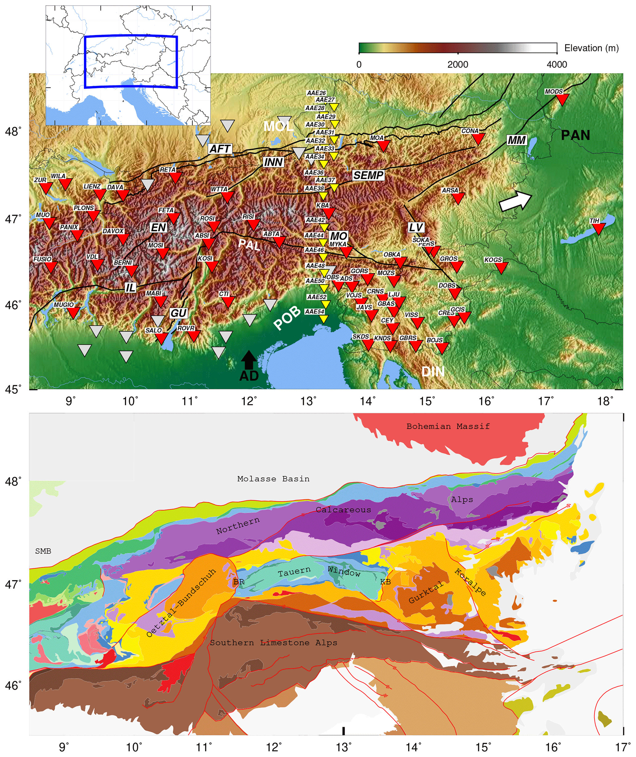
Figure 1 Study region in the Eastern and Southern Alps. Top: permanent stations are marked in red and grey, and the 19 EASI stations used are shown in yellow. Main faults of the region are represented by black lines. The faults are indicated as follows. AFT: northern Alpine Front Thrust, INN: Inntal, SEMP: Salzach–Ennstal–Mariazell–Puchberg, MM: Mur–Mürz, LV: Lavant Valley, MO: Mölltal, GU: Giudicarie, IL: Insubric, EN: Engadine, PAL: Periadriatic line. MOL: Molasse Basin, PO: Po Basin; PAN: Pannonian basin. DIN: Dinarides mountain belt. The black arrow shows the convergence vector of the Adriatic Plate (AD) with respect to the European Plate (EU). A white arrow illustrates the direction of eastward escape of the Alcapa tectonic block (see Sect. 6.4). After the different selection criteria, the stations shown in red and yellow were entered into the inversion (see text). Bottom: tectonic map of the study region (Schmid et al., 2004, 2008, from http://www.spp-mountainbuilding.de, last access: 17 September 2020). Units discussed in the text are labeled on the map. SMB: Swiss Molasse Basin, BR: Brenner fault, KB: Katschberg fault. Red lines represent the faults.

In this study, we investigate the crustal structure of the Eastern and Southern Alps (Fig. 1) with ambient noise tomography. The European Alps resulted from N–S convergence of the Adriatic and European plates since the late Cretaceous time and Adria–Europe collision since late Eocene to Oligocene time (Schmid et al., 2004; Handy et al., 2010, 2015). The complex, non-cylindrical structure of the Eastern Alps and eastern Southern Alps (Schmid et al., 2013; Rosenberg et al., 2018) reflects the interplay between orogen-normal shortening and orogen-parallel motion during oblique indentation of Europe by the Adriatic microplate in the Miocene time (Scharf et al., 2013; Handy et al., 2015; Favaro et al., 2017). Adria moved to the north and rotated counterclockwise with respect to Europe (Le Breton et al., 2017) such that indentation was partly accommodated by NNW–SSE shortening in the eastern Southern Alps (e.g., Schonborn, 1992) and partly by upright folding and eastward tectonic escape of the eastern Alpine orogenic crust (Ratschbacher et al., 1991a; Scharf et al., 2013; Schmid et al., 2013). This escaping orogenic crust is bounded by strike-slip faults (Periadriatic, Salzach–Ennstal–Mariazell–Puchberg – SEMP, Inn Valley, Mur–Mürz, and Lavant Valley faults; e.g., Linzer et al., 2002; Schmid et al., 2004) and low-angle normal faults (Brenner and Katschberg faults) at either end of the Tauern Window (Selverstone, 1988; Genser and Neubauer, 1989; Scharf et al., 2013, 2016).

On the lithospheric scale several study methods such as seismic tomography, anisotropy, and receiver functions have assessed the structures and proposed models of slab anomalies and geometry (Lippitsch et al., 2003; Schmid et al., 2004; Kissling et al., 2006; Mitterbauer et al., 2011; Karousová et al., 2013; Bianchi et al., 2014; Handy et al., 2015; Qorbani et al., 2015; Hua et al., 2017; Rosenberg et al., 2018; Hetényi et al., 2018b; Kästle et al., 2019). However, despite wide-angle reflection–refraction experiments (Bleibinhaus and Gebrande, 2006; Gebrande et al., 2006; Behm et al., 2007a; Brückl et al., 2007, 2010) and local earthquake tomography (Diehl, 2008) targeting the crust, the velocity structure of the Eastern Alps is still not fully understood. This is due to the low level of seismicity in the region and insufficient local earthquake data to perform traditional tomographic studies, as well as to the limits of active seismic experiments covering the region. Therefore, ambient noise tomography appears to be perfectly suited to study crustal structure in this area.

Prior to this study, parts of the Alps and their surroundings were seismically imaged with noise-based tomography that provided Rayleigh-wave group velocity maps (Stehly et al., 2009; Verbeke et al., 2012). These formed a database of surface-wave group and phase velocity dispersion curves that were inverted to derive both group and phase velocity maps of central Europe. Molinari et al. (2015) used the database of Verbeke et al. (2012) to derive a 3D shear velocity model of the Alpine region and Italy. The Western Alps have also been studied with ambient noise tomography (Fry et al., 2010), which yielded isotropic and anisotropic models of surface-wave phase velocity. Using surface-wave tomography from ambient noise and earthquake data, Kästle et al. (2018) presented a shear velocity model of the Alps. Lu et al. (2018) also used ambient noise data to present a shear velocity model of the European crust and upper mantle. To the east of the Eastern and Southern Alps (ESA), the crustal structure of the Carpathian–Pannonian region was studied with noise tomography depicted in surface-wave group velocity and 3D shear velocity maps (Ren et al., 2013). Behm et al. (2016) applied ambient noise tomography to data from the ALPASS project to study the crust of the Eastern Alps, presenting Rayleigh- and Love-wave group velocity maps and a shear velocity model. However, the results of Ren et al. (2013) and Behm et al. (2016) are limited to the profiles used in those studies.

Although the area of this study is included in two recent shear velocity models (Kästle et al., 2018; Lu et al., 2018), little attempt has been made to interpret those velocity models with regard and in comparison to surface geology and smaller-scale features. In this study, we therefore focus on the crustal structures of the Eastern Alps and Southern Alps. We present a new local high-resolution 3D shear velocity model of the region using cross-correlation of seismic ambient noise. To augment the recent shear velocity models (e.g., Lu et al., 2018), we derive a (group) velocity map for both Rayleigh and Love waves and present separate shear velocity models from Rayleigh- and Love-wave velocities for the ESA. We then discuss our new models for the uppermost 40 km of the crust with respect to the geologic and tectonic features.

2 Data and analysis

2.1 Ambient noise data

We used continuous three-component seismic data recorded at 71 permanent broadband stations in the Eastern and Southern Alps from the Seismic Network of Austria (OE, 1987), National Seismic Network of Switzerland (CH, 1983), Italian Seismic Network (INGV, 2006), Province Südtirol (SI, 2006), German Regional Seismic Network (GR, 2001), BayernNetz, Germany (BW, 2001), Slovenian Seismic Network (SL, 2001), Hungarian National Seismological Network (HU, 1992), and Slovak National Network of Seismic Station (SK, 2001). In order to improve ray coverage, we completed our dataset with 19 temporary broadband stations of the AlpArray-EASI project (AlpArray, 2015; Hetényi et al., 2018a). The Eastern Alpine Seismic Investigation (EASI) is a collaborative seismological project that was the first AlpArray collaborative experiment between the Swiss Federal Institute of Technology, University of Vienna (Austria), and the Academy of Sciences of the Czech Republic; it ran between July 2014 and July 2015. In that project, seismic stations were deployed along a north–south profile, roughly along longitude 13.5^∘ E, from the internal Bohemian Massif to the Adriatic Sea with inter-station distances between 10 and 15 km. Using the 19 EASI stations improved station coverage, especially in the central Eastern Alps where the station density is relatively low. After applying several selection criteria (see Sect. 2.3.) to the computed cross-correlation functions, 79 stations were selected for the tomography (see Fig. 1).

2.2 Waveform preprocessing

The first step of any noise-based analysis requires preprocessing the continuous waveform data, which strongly affects the quality of cross-correlation functions, dispersion curves, and the resulting velocity maps. Because noise characteristics and station configurations differ for each study, no universal preprocessing methodology exists. The best methodology and the various processing steps have to be tested for each dataset and are usually evaluated with basic parameters such as the symmetry of the cross-correlation function, signal-to-noise ratio, and frequency bandwidth (e.g., Bensen et al., 2007; Poli et al., 2013). Here, we tested several classical preprocessing methods including windowing (e.g., Seats et al., 2012), whitening (e.g., Bensen et al., 2007), and 1 bit normalization (e.g., Cupillard and Capdeville, 2010). The processing scheme chosen maximizes the signal-to-noise ratio (SNR), defined here as the peak amplitude divided by the standard deviation of the noise. Our final preprocessing methodology follows Zigone et al. (2015) and consists of the following steps: (1) removing the instrument responses, high-pass filtering at 125 s, and glitch correction by clipping the data at 15 standard deviations; (2) removal of the transient signals (e.g., earthquakes) by cutting the daily records into 2 h segments on which we perform an energy test: when the energy of a segment is greater than twice the standard deviation of the energy of the 24 h (daily) record, the 2 h segment is removed. (3) Ambient noise is not spectrally white, which may induce an amplitude bias in the resulting cross-correlations (e.g., Rhie and Romanowicz, 2004; Bensen et al., 2007). The noise spectrum is therefore normalized using a whitening function by dividing the amplitude by its absolute value between 1 and 100 s periods without changing the phase. (4) We also perform a second clipping step in order to ensure that all the energy from transient sources that were not previously deleted by the energy test, such as small earthquakes, is properly removed from the waveforms. This is done by clipping amplitudes larger than 4 standard deviations of the whitened records. (5) Finally, the data are down-sampled to 4 Hz to reduce computational costs.

2.3 Computing cross-correlation functions

After preprocessing of the waveform, we compute cross-correlation functions for all station pairs, which resulted in 4005 cross-correlations from 90 stations. The cross-correlation for each daily record and each station pair is computed over all possible combinations of three-component data, vertical (Z), north–south (N), and east–west (E). This yields nine inter-components, ZE, ZN, ZZ, EE, EN, EZ, NE, NN, and NZ, constituting the correlation tensor. The ambient noise in the microseism frequency band is dominated by surface waves (Shapiro and Campillo, 2004; Shapiro et al., 2005); using all nine of these inter-components of cross-correlation enables us to construct both Rayleigh and Love waves from the computed cross-correlation. The correlation tensor consists of nine inter-components: RR, RT, RZ, TR, TT, TZ, ZR, ZT, and ZZ. Rayleigh waves emerge from the RR, RZ, ZR, and ZZ, and Love waves emerge from the TT. The cross-terms (TR, RT, ZT, TZ) also carry some weak diffuse energy without any clear arrivals, which confirms the quality of the correlation component rotations. The correlation tensor representing the propagation of surface waves through all station pairs is shown in Supplement Fig. S1.

Cross-correlations are computed in the frequency domain and then returned to the time domain to be stacked over the 2 years of data in order to reduce the seasonal effect of the noise source in the cross-correlation. Rotation of the stacked cross-correlation was then performed based on the azimuth between the station pairs to obtain the cross-correlation on the radial (R), transverse (T), and vertical (Z) components, which form a nine-inter-component correlation tensor including RR, RT, RZ, TR, TT, TZ, ZR, ZT, and ZZ. In order to select the clearer cross-correlation, we picked those that have signal-to-noise ratio (SNR) larger than 4. The SNR is calculated as the maximum amplitude of cross-correlation divided by the standard deviation of a noise window. We found that cross-correlations with a low SNR can be associated primarily with certain stations, marked in grey in Fig. 1. We therefore removed those 11 stations, which resulted in 23 % less cross-correlation. Figure 2 shows examples of 2-year (2014–2015) stacked and rotated cross-correlations, with the corresponding station path shown in the top panel. Examples present long inter-station distances between CEY-DAVOUX and CONA-KNDS, as well as short station distances between FETA-ROSI and AAE26-AAE31. Only ZZ, ZR, RZ, RR, and TT are shown in the figure as Rayleigh and Love waves are extracted from these five inter-components (Shapiro and Campillo, 2004).

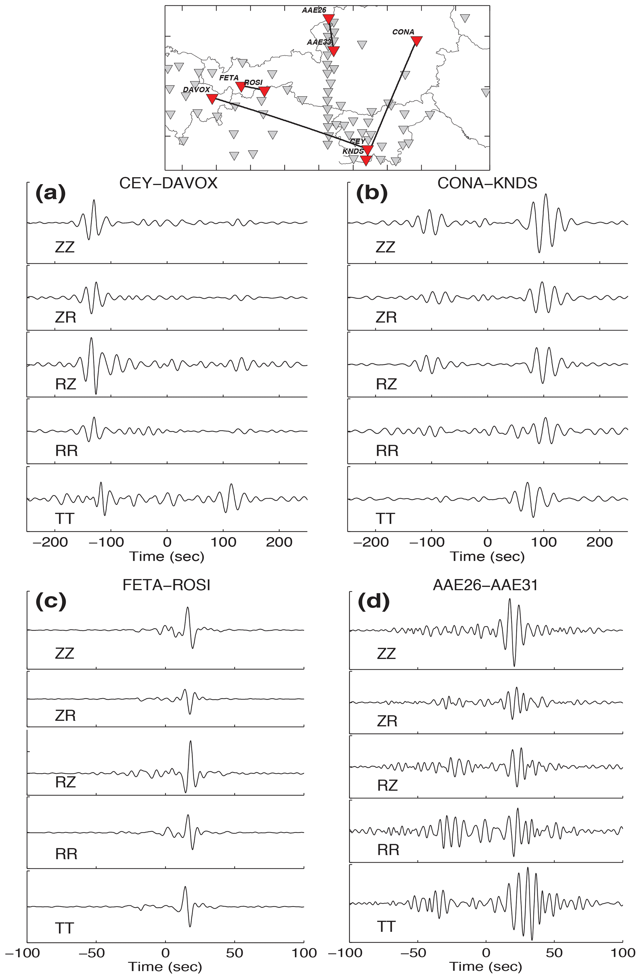
Figure 2 Examples of stacked and rotated cross-correlations from 2 years of data (2014–2015). The top panel shows the inter-station paths and geometry. CEY-DAVOUX and CONA-KNDS represent long inter-station distance, while FETA-ROSI and AAE26-AAE31 are within a short distance.

The examples shown in Fig. 2 were chosen based on the station geometry and location with respect to the North Atlantic and the North Sea coastline, which should be the dominant noise source for our study region (e.g., Yang and Ritzwoller, 2008; Juretzek and Hadziioannou, 2016). We observe that for pairs parallel to the North Sea coastline, the cross-correlations are slightly asymmetric, with larger amplitudes for propagation directions arriving from the north and northeast. This can be seen at CONA-KNDS (Fig. 2b) and AAE26-AAE31 (Fig. 2d), for which the surface-wave amplitude is larger on the causal side. When station pairs are nearly normal to the North Sea coastline, such as CEY-DAVOX (Fig. 2a) and FETA-ROSI (Fig. 2c), we obtained strongly asymmetric cross-correlation. The differences between causal and acausal parts in the coast-normal station pairs are larger than the coast-parallel cases. Propagation directions from the North Sea coastline (from the northwest) result in large amplitudes, as can be seen in the propagation direction from DAVOX to CEY and from FETA to ROSI (Fig. 2). This supports the hypothesis that seismic ambient noise is mainly generated by the interaction of the ocean swells with the seafloor located north and northwest of Europe. It also suggests that less energy is coming from southerly directions with respect to the northerly directions.

3 Dispersion measurements

High-quality cross-correlations are mandatory to measure accurate group velocity dispersion curves. Quality checks of the cross-correlation based on SNR is one of the key tasks for preparing clear and reliable cross-correlations and obtaining acceptable empirical Green's functions (Bensen et al., 2007). That step removes poor-quality cross-correlations, which is critical when using an automatic procedure for dispersion measurement. In order to improve the reliability of the dispersion measurements we stack the causal and acausal side of the correlation function to obtain a single cross-correlation for each station pair (Bensen et al., 2007). Such a procedure also broadens the frequency content of the merged cross-correlation by combining the different frequency content of opposite propagation directions (Yang and Ritzwoller, 2008; Shapiro and Campillo, 2004; Verbeke et al., 2012), which helps the following travel time measurements.

We measured the group velocity dispersion of the fundamental mode of the Rayleigh and Love waves for periods between 1 and 50 s using frequency–time analysis (FTAN) (Levshin and Ke\ĭlis-Borok, 1989). To improve the reliability of Rayleigh-wave dispersion measurements we used the redundancy of the correlation tensor by using all components (RR, RZ, ZR, and ZZ) containing Rayleigh waves. FTAN is first computed for each component i independently to obtain a normalized period–group velocity diagram N_i(T,u); u is the group velocity and T the period. Applying a logarithmic stacking in the period–group velocity domain (Campillo et al., 1996), as $A_{\mathrm{s}}(T,u)={\prod }_i{N}_i(T,u)$, we then combined the four RR, RZ, ZR, and ZZ components and formed a product of these four components for each station pair; the amplitude of A_s(T,u) is dependent on the standard deviation of the group velocities. We evaluated the final dispersions on a $\left[A_{\mathrm{s}}\right(T,u){]}^{\frac{\mathrm{1}}{i}}$ diagram, which allows us to obtain a normalized period–group velocity diagram with amplitude between 0 and 1. The normalized period–group velocity diagram makes us able to select good-quality dispersion measurements according to the amplitude. Here we selected the period velocity values that have at maximum amplitude greater than 0.07. Examples of two period–group velocity diagrams are presented in Fig. 3 for stations MOSI-SALO and ABTA-CONA. The dispersion curves are shown by the white line in the figure. The same procedure was applied to get the Love-wave dispersion curves using only the TT component. See Supplement Fig. S2 for more examples of period velocity diagrams.

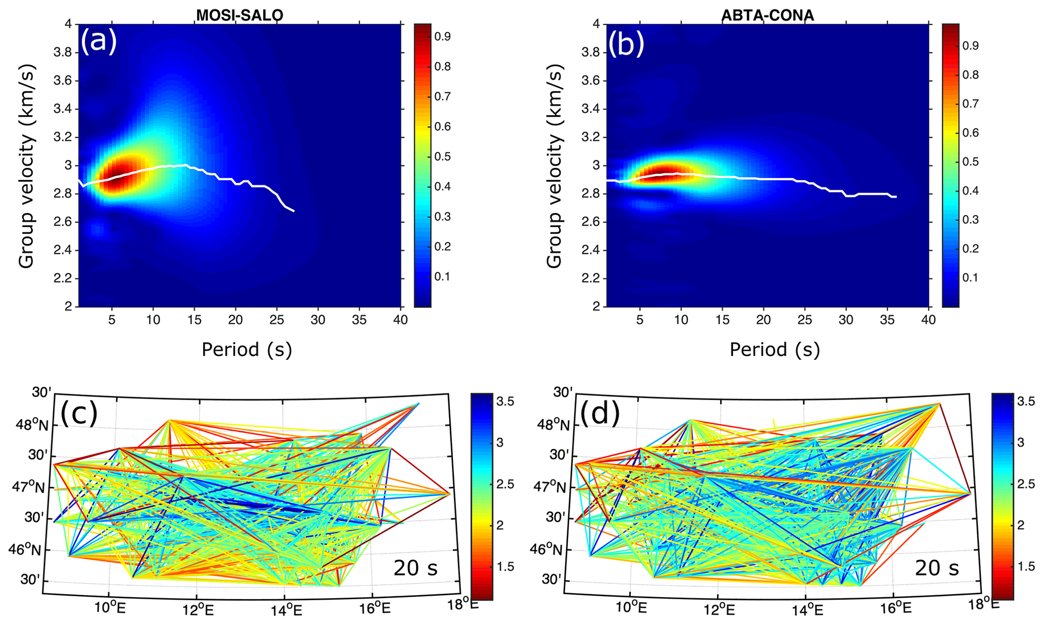
Figure 3 (a, b) Example of a normalized period–group velocity diagram from (a) MOSI-SALO and (b) ABTA-CONA. The white line represents the extracted dispersion curve. (c, d) Example of velocity measurements at a 20 s period for (c) Rayleigh waves and (d) Love waves. Note that stable high- and low-velocity zones can be seen in the velocity measurements. See Supplement Fig. S2 for more examples of period–group velocity diagrams.

To increase the quality of the velocity measurements, we applied a number of criteria: (1) to avoid high ray-path density in the central area with respect to other parts of the region, we removed all combinations of temporary–temporary inter-stations and kept only the temporary–permanent pairs. (2) We removed all paths with inter-station distances smaller than 2 wavelengths at each period. (3) We applied a second SNR pass (SNR > 5) for the correlations to pass the velocity measurements to ensure that we obtain well-estimated travel times. (4) We exclude velocity measurements that were not in a range within 2 standard deviations of the mean velocity for a given period.

Applying those criteria, the dispersion data for each period were extracted to be inverted to group velocity maps. Figure 3 shows an example of velocity measurements obtained at a 20 s period for Rayleigh and Love waves. The stations and paths that satisfied our criteria are shown on the map. The measurements directly show high- and low-velocity anomalies, which are spatially stable and related to the crystalline core zone of the Alps and the sedimentary basins, respectively. The period dependence of the signal-to-noise ratio (SNR) of the dispersion measurements after applying the abovementioned criteria is represented in Fig. 4. Rayleigh waves are extracted from the ZZ, RR, ZR, and RZ inter-components, and Love waves appear on the TT inter-components. In addition to the average SNR for Rayleigh and Love waves for all station pairs, the average SNRs of those inter-components are also shown in Fig. 4. The number of measurements selected for each period used in the inversions is presented in Supplement Table S1.

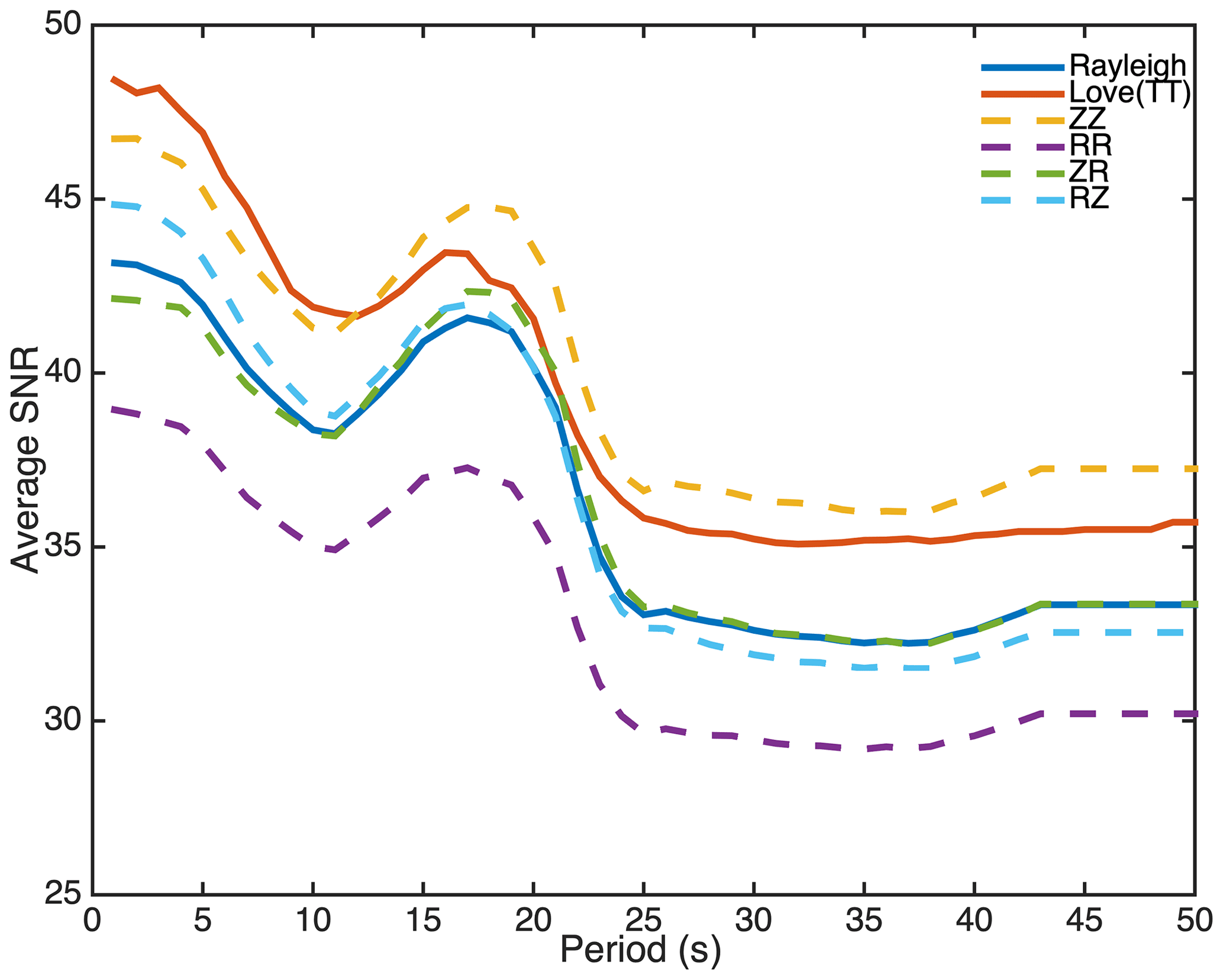
Figure 4 Average signal-to-noise ratio (SNR) for Rayleigh and Love waves for all station pairs. Average SNRs of ZZ, RR, ZR, and RZ are also shown; Rayleigh waves are extracted from these four inter-components. Average SNRs of TT and Love waves are also represented in the figure. Love waves appear on the TT inter-components.

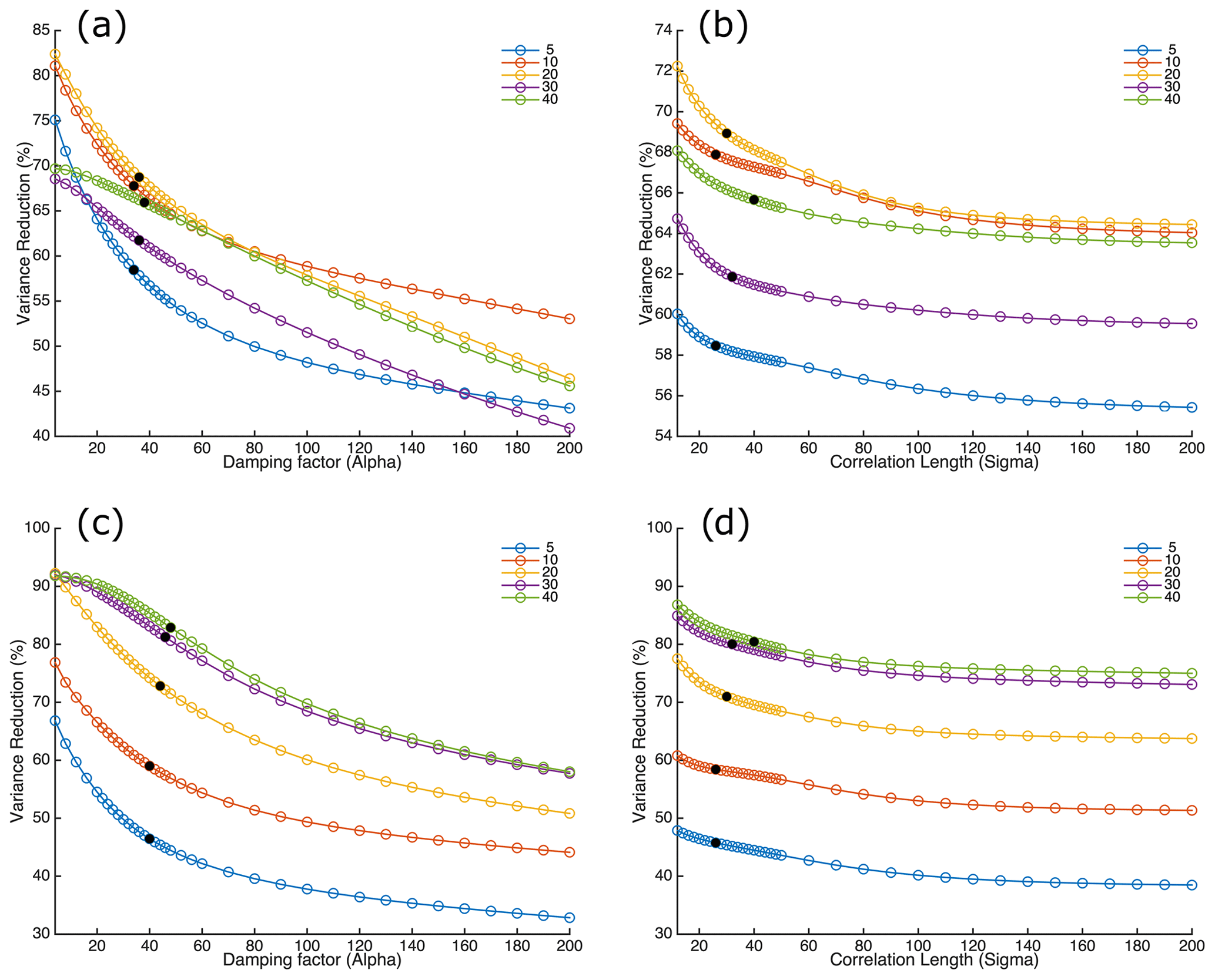
Figure 5 Variance reduction as a function of the inversion parameters. (a) L-curve analysis for damping factor (α) for Rayleigh waves at periods of 5, 10, 20, 30, and 40 s. (b) Correlation length (σ) for Rayleigh waves in the same period range. (c, d) Variance reduction vs. damping factor and correlation length, respectively, for Love waves in the same period range. The selected parameters are shown by black circles.

4 Group velocity tomography

We used the method of Barmin et al. (2001) to invert the dispersion data and to derive tomographic images of surface-wave group velocity. The standard forward problem is given in matrix notation as d=Gm, where $d=t_{\mathrm{obs}}-t_{\mathrm{mod}}$, defined as the difference between observed and modeled travel time. The matrix G is travel times in each cell of the initial model for each path. The goal is to find the group velocity model as $m=(u-u_{\mathrm{0}})/u_{\mathrm{0}}$, where u₀ is the initial velocity and u is the velocity after the inversion. The method is a damped least-squares inversion based on minimization below a penalty function,

$$\begin{array}{}\text{(1)}& \left(G\right(m)-\mathrm{d}{)}^T.(G\left(m\right)-\mathrm{d})+{\mathit{\alpha }}^{\mathrm{2}}{∥F\left(m\right))∥}^{\mathrm{2}}+{\mathit{\beta }}^{\mathrm{2}}{∥H\left(m\right)∥}^{\mathrm{2}},\end{array}$$

which consists of a linear combination of data misfit, model smoothness F, and the magnitude of perturbations. F is a Gaussian spatial smoothing function over 2D grids(s), with correlation length σ calculated as

$$\begin{array}{}\text{(2)}& F\left(m\right)=m\left(r\right)-\underset{\mathrm{s}}{\int }\exp \left(-{\displaystyle \frac{{\left|r-r^{\prime }\right|}^{\mathrm{2}}}{\mathrm{2}{\mathit{\sigma }}^{\mathrm{2}}}}\right)m\left(r^{\prime }\right)\mathrm{d}{r}^{\prime },\end{array}$$

and function H defined as $H\left(m\right)=\exp (-\mathit{\lambda }\mathit{\rho })m$, where λ is a weight factor and ρ defines the path density. The magnitude of the model perturbation is controlled by two parameters, defined as λ and β. If the ray coverage is relatively good, these two parameters do not affect the final model (e.g., Stehly et al., 2009; Poli et al., 2013; Zigone et al., 2015), which is the case for our study region. Therefore, we fix λ and β at 0.4 and 3, respectively. The spatial Gaussian smoothing is controlled by a damping factor (α) and the width of smoothing area (σ, also called correlation length in kilometers). These parameters strongly affect the variance reduction of the final model. Stehly et al. (2009) recommended that the correlation length should be at least equal to grid size.

Using a grid size of 16 km, we tested several values for the correlation length (σ) and damping factor (α), performing an L-curve analysis (e.g., Hansen and O'Leary, 1993; Stehly et al., 2009). Figure 5 shows variation of variance reduction of the models with respect to correlation length (σ) and damping factor (α) for a selection of periods. Based on the variation of the variance reduction for each period range, and for Rayleigh and Love waves separately, optimized values for α and σ were selected. These values are between 44 and 50 for damping factor and between 20 to 34 for correlation length (Supplement Table S2 shows the values selected for α and σ for each period range). After selection of our optimized parameters, the inversion for group velocity was performed using an initial model of the average group velocity at each period.

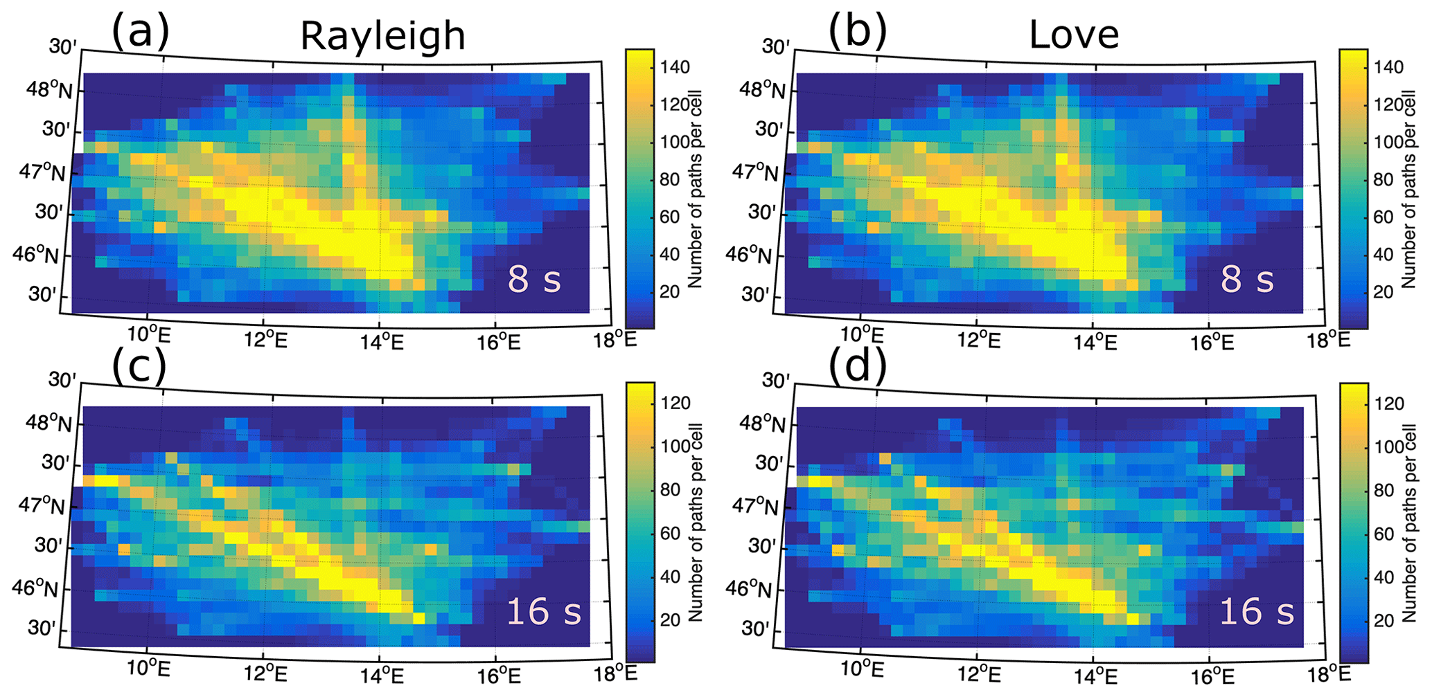
Figure 6 Path density map for the tomography inversion: (a, c) for Rayleigh waves at 8 and 16 s, respectively and (b, c) for Love waves at 8 and 16 s. The path coverage is generally good for the entire region. Most of the cells have a path density more of than 20 rays per cell. Path density maps at larger periods are also shown in Supplement Fig. S3.

4.1 Resolution of tomography

We assessed the spatial averaging of the tomography inversion results in two ways.

1. The first is through the path density at each cell used for the inversion. Figure 6 presents the path density map at 8 and 16 s for both Rayleigh and Love waves (path density maps at larger periods are also presented in Supplement Fig. S3). The path coverage of the region is good for most of the cells, with a path density above 20. The path coverage reaches 120 paths per cell in the Southern Alps and in the Tauern Window, particularly for periods shorter than 15 s. At the edges of the study region the resolution decreases rapidly due to fewer stations and less ray coverage (see Fig. 6).

2. The second is by quantifying the dependence of the group velocity at each cell on the other cells (Barmin et al., 2001), which gives an estimation of the correlation length or the size of the averaging spot for each cell of the model. That was done via the resolution matrix, which depends mainly on the distribution of high-quality velocity measurements (path coverage, Fig. 6) and on the network geometry. The spatial averaging is evaluated by plotting the correlation length, defined here as the distance in kilometers, for which the value of the resolution matrix decreased to half. As the spatial projections of the individual resolution matrices for each cell are not symmetric, a best and a worst direction exist. Figure 7 shows the map of the correlation length of the final velocity model for Rayleigh (left) and Love (right) waves at 20 s. We show the correlation length in the best direction (Fig. 7a and  7d), the mean correlation length (Fig. 7b and  7e), and the correlation length in the worst direction (Fig. 7c and  7f) for each cell. In the best direction (Fig. 7b), the size of the averaging spots is about 16–30 km for most of the study region. In the worst direction (Fig. 7c), the correlation length still reaches 30 km in the center but increases rapidly above 80 km at the edges. The mean correlation length is ∼ 20 km in the center of the study region and ∼ 50–60 km at the edges (Fig. 7b). Based on those analyses, our tomographic inversion will be able to differentiate two different structures that span at least two cells (32 km length) for most of the study area. Although fewer cross-correlations are used to reconstruct the Love waves than the Rayleigh waves, the path density and correlation length obtained for the Love waves remain more or less on the same order as those of the Rayleigh waves, which is sufficient to resolve the expected geological features.

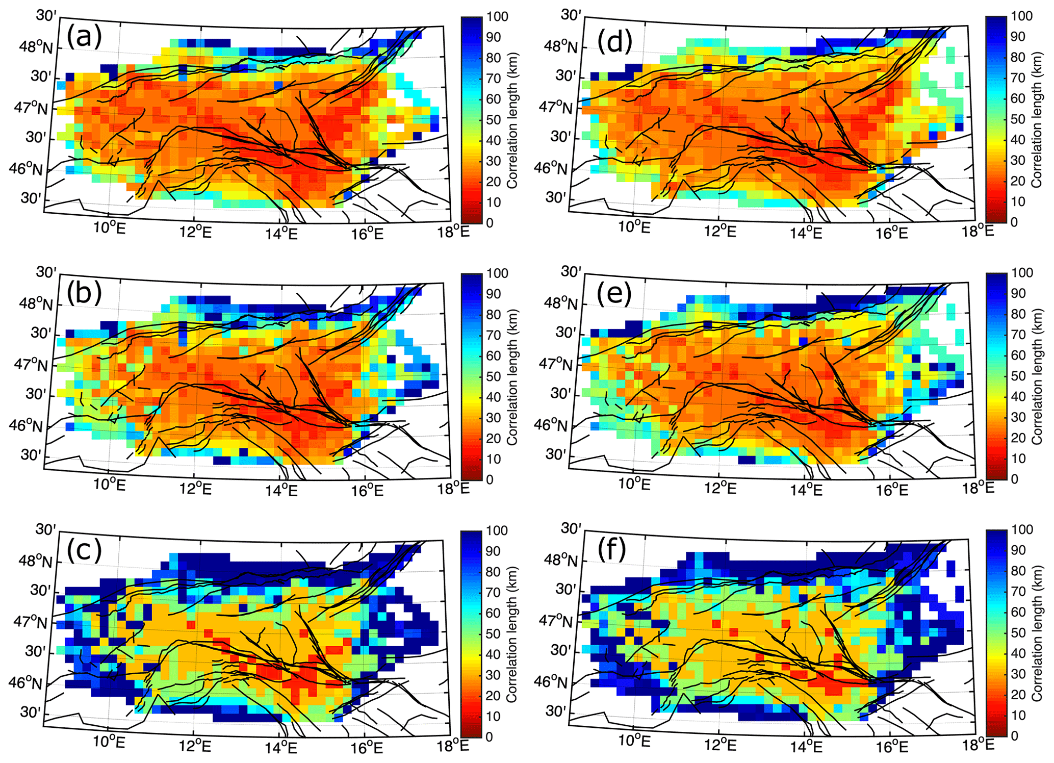
Figure 7 Resolution of the group velocity inversion shown via correlation length maps for a 20 s center period. Colors show the correlation length, e.g., the distance for which the value of the resolution matrix decreases to half. Rayleigh waves: (a) correlation length in the best direction. (b) Mean correlation length for each cell. (c) Correlation length in the worst direction. Love waves: (d) correlation length in the best direction. (e) Mean correlation length for each cell. (f) Correlation length in the worst direction.

4.2 Group velocity maps

Figures 8 and 9 show the group velocity maps at periods of 5, 10, 15, and 20 s. In general, both Rayleigh- (Fig. 8) and Love-wave (Fig. 9) group velocity maps present similar features and correlate well with surface geology, particularly at upper crustal depths. To assess the velocity pattern with respect to the geological units, we extracted their borders from the geological map of Austria (Egger et al., 1999, Supplement Fig. S4) and the tectonic map of the Alps (Fig. 1, Schmid et al., 2004). The borders are shown as dashed lines in Figs. 8 and  9, representing the margins of the two dolomite units to the south (Southern Limestone Alps, SLA) and to the north (carbonates of the Northern Calcareous Alps, NCA), the crystalline core zone of the Alps (CZA) in between (Fig. 1), and the Tauern Window (TW) of the Eastern Alps (yellow dashed lines in Figs. 8 and  9). The CZA is well-marked by the broad high-velocity anomalies extending from the west to the east of the region. The SLA and the NCA are also marked by low velocities. At 5 and 10 s periods, the eastern border of the CZA matches the group velocity contrast (no. 1 in Fig. 8a). The southern margin of the CZA, particularly its western part, is clearly fitted by the edge of the high-velocity anomaly in that area at 5 to 10 s (no. 2 in Fig. 8a).

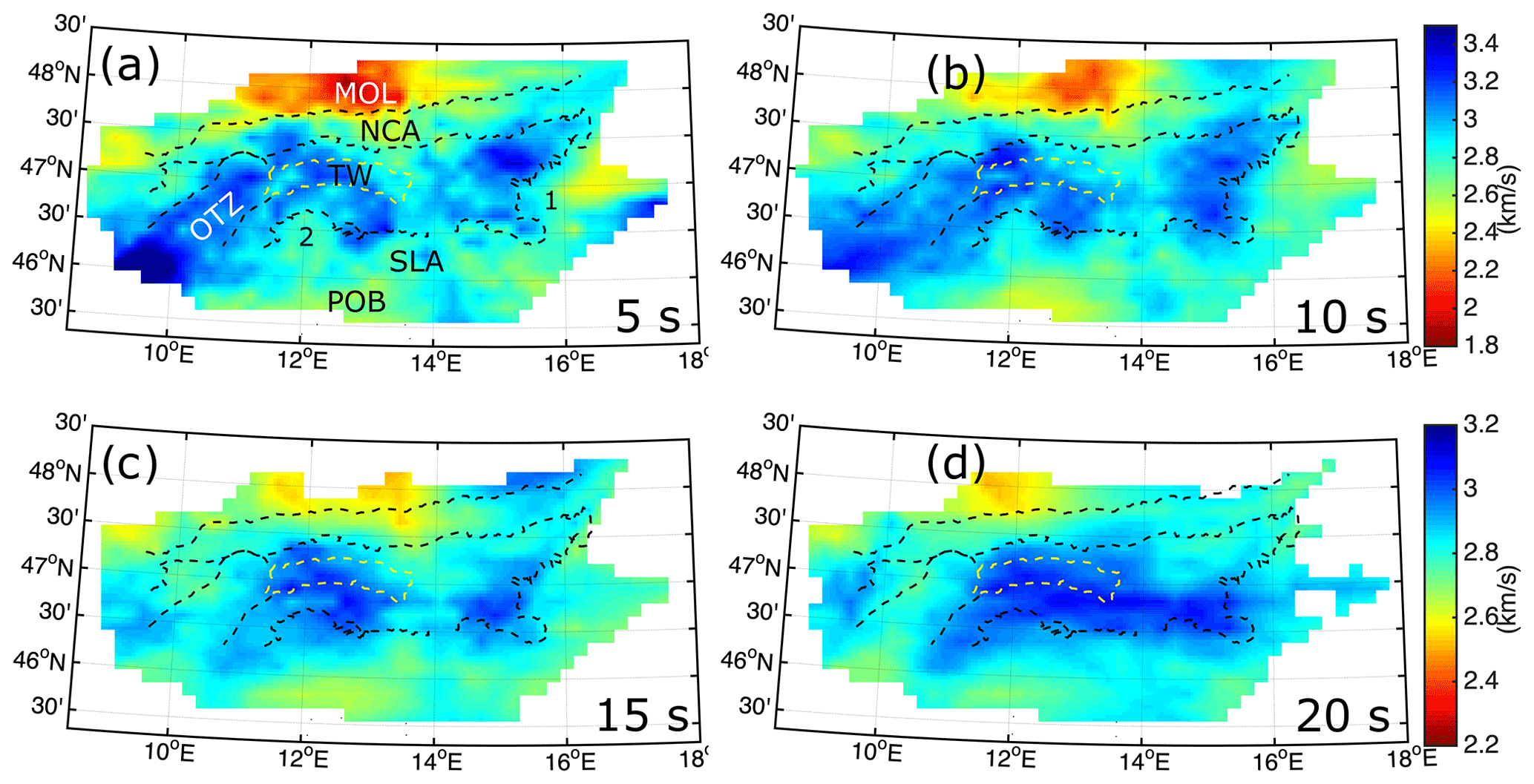
Figure 8 The obtained Rayleigh-wave group velocity maps at periods of 5, 10, 15, and 20 s. Dashed lines (Egger et al., 1999; Schmid et al., 2004, see Fig. S4) represent the margins of the Northern Calcareous Alps (NCA), the crystalline core zone of the Alps (CZA), the Ötztal block (OTZ), and the Tauern Window (TW). The eastern margin of the CZA (no. 1 at 5 s) and the northern margin of the Southern Limestone Alps (SLA; no. 2 at 5 s) are well-marked by the velocity contrast at 5 s. MOL: Molasse Basin, POB: Po Basin. Group velocity maps at larger periods of 30 and 40 s are presented in Supplement Fig. S5.

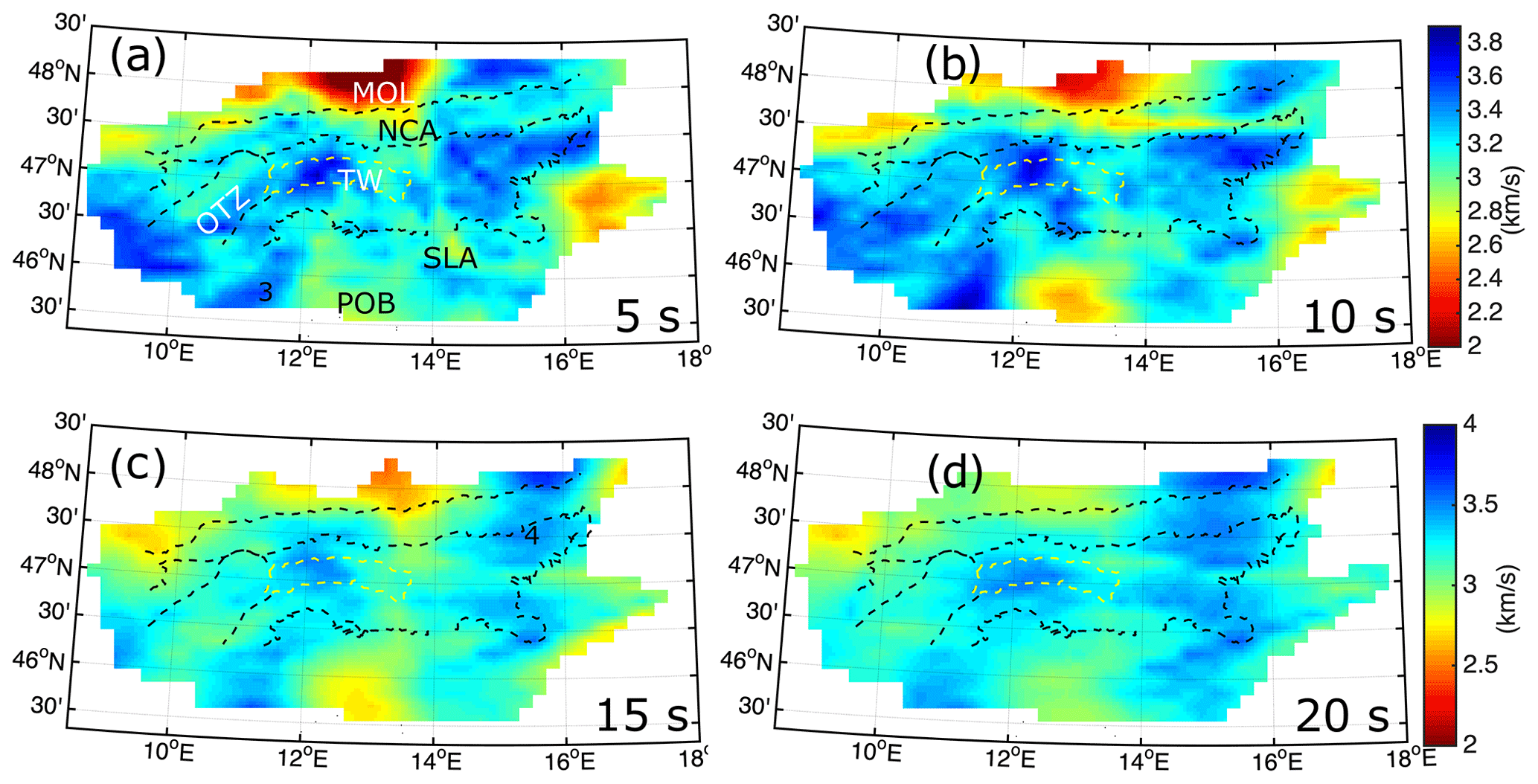
Figure 9 The obtained Love-wave group velocity maps at periods of 5, 10, 15, and 20 s. See Fig. 9 caption for abbreviations. No. 4 at 15 s shows a notable high-velocity anomaly in the easternmost part of the Northern Calcareous Alps (NCA). CZA: crystalline core zone of the Alps, OTZ: Ötztal block, TW: Tauern Window, MOL: Molasse Basin, POB: Po Basin, SLA: Southern Limestone Alps.

A high-velocity zone is featured in the easternmost part of the CZA at 5, 10, and 15 s. This feature might be associated with the Koralpe–Wölz high-pressure nappe system, the area on both sides of the Lavant Valley transform fault, which consists of eclogite facies and has the age of the Alpine tectono-metamorphic event of 90–110 Ma (Bousquet et al., 2012). The late Cretaceous (Eoalpine) Ötztal–Bundschuh and Silvretta metamorphic basement nappes are also perfectly imaged by high-velocity zones (shown as OTZ on Fig. 8a and b). At periods greater than 10–12 s, the OTZ no longer appears on the group velocity map, which may indicate the depth extent of the OTZ. A high-velocity anomaly is observed in the western part of the TW, while its eastern part shows lower velocities.

Figure 9 shows Love-wave group velocity maps. As expected, the Love wave presents higher velocities than the Rayleigh wave, as noted by the difference between color scales in Figs. 8 and 9. Similar to the pattern of the Rayleigh-wave group velocity, the CZA is well-marked by the Love-wave high-velocity anomaly bounded by the two dolomite provinces (Fig. 9a) to the north and to the south. The TW is also marked by high-velocity anomalies at most of the periods. However, similar to Rayleigh waves, the western part of the TW shows higher velocity. There is a velocity increase to the west of the Po Basin at ∼ 11^∘E (no. 3 in Fig. 9a), which becomes more pronounced at the 10 s period. This might be associated with the depth extent of the magmatic rocks under the southern Alpine sediments (Dolomites in the Trentino region, Italy). At the 15 s period, a pronounced high-velocity anomaly occurs in the easternmost part of the NCA (no. 4 in Fig. 9c). A similar anomaly appears in the velocity model of Behm et al. (2016). The Molasse and Po Basin (Fig. 1) can be clearly located on both Rayleigh- and Love-wave group velocity maps (Figs. 8 and 9). The OTZ metamorphic units are marked partly by the Love waves at the 5 s period (Fig. 9a). Further discussion of this feature will be provided in Sect. 6 when describing the shear-wave velocity model.

5 Shear-wave velocity inversion

In order to derive a 3D shear velocity (Vs) model of the region, we performed a Vs depth inversion using the linearized inversion procedure of Herrmann (2013). We first constructed local dispersion curves from the group velocity maps at each cell (16×16 km) of the grid. These local dispersion curves are inverted to obtain local 1D shear velocity models at each cell, which are finally combined to provide a 3D shear velocity model for the region. We excluded the group velocities of periods smaller than 4 s since measuring the group velocity of the fundamental mode of the surface waves at those periods could easily be mistaken for higher modes. We also did not use periods larger than 42 s because of the lower number of measurements. As the inversion scheme is linearized, the accuracy of the final model strongly depends on the initial velocity model. To construct a good initial model, we used a three-step approach: (1) we extracted an average dispersion curve using all cells with more than five paths; (2) the average dispersion curve is inverted using a 1D starting model proposed by Behm et al. (2007a); (3) finally, the resulting average Vs model is used as a starting model for the inversion of the local dispersion curves in each cell of the grid. The parametrization is made for 30 layers of 2 km thickness above a half-space. Shear velocities range from 3 km s⁻¹ in the top layer to 4.5 km s⁻¹ in the half-space. During the inversion, no restriction was applied for Moho depth; there was also no layer weighting, and no fixed velocity was set. The velocity is allowed to take a large range of values as long as the depth variation is smooth. We performed 30 iterations for the inversion, which was sufficient to achieve a reasonable fit. The first two iterations were done with higher damping in order to not overshoot the model; the other 28 iterations were performed with a lower damping factor. As discussed below, the inversion results are well-defined solutions given the model parameterization.

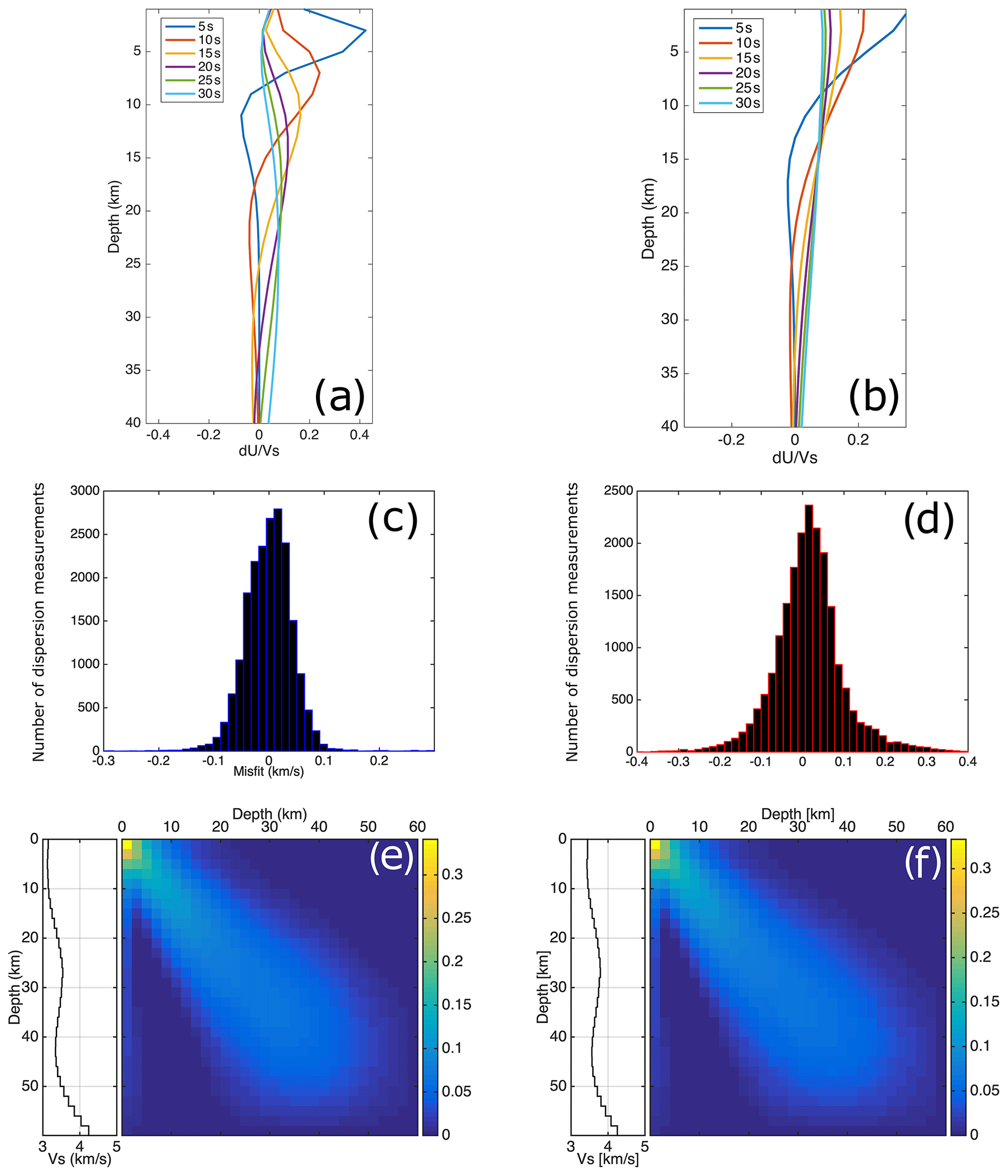
Figure 10 Depth sensitivity kernels for Rayleigh (a) and Love waves (b) for a selection of periods. Histograms of the distribution of misfit between synthetic and observed dispersion curves for the Rayleigh-wave (c) and Love-wave (d) shear velocity model at all periods. The misfit of the Rayleigh-wave model (RVs) is generally less than 0.1 km s⁻¹, and for the Love-wave model (LVs) it is less than 0.25 km s⁻¹ (see text). (e) The resolution matrices of the average velocity model derived from Rayleigh waves and (f) from Love waves. The left-hand side of panels (e) and (f) shows the average 1D velocity model for the region.

Figure 10 shows the average velocity model obtained from Rayleigh- and Love-wave average dispersion curves. We used this 1D average velocity model as the initial model to invert the local dispersion curves in order to obtain the best-fitting local 1D velocity model at each cell. Depth sensitivity kernels for a selection of periods used in the inversion are presented in Fig. 10. The kernels are shown for both Rayleigh- and Love-wave fundamental-mode group velocities. The distribution of misfit between the theoretical and estimated dispersion curves of the models at all periods is also presented in Fig. 10, showing small misfit usually below ±0.1 and ±0.25 km s⁻¹ for Rayleigh (Fig. 10c) and Love waves (Fig. 10d), respectively. The depth resolution of the inversion can be assessed through the normalized resolution matrix of the computed model, which is shown in Fig. 10 for the Rayleigh and Love average models. Both Rayleigh and Love waves allow for a good resolution above ∼42 km of depth, where the resolution matrices are symmetric (Fig. 10). The final shear velocity models obtained from the Rayleigh-wave group velocity are presented in Fig. 11, and those from Love waves are presented in Fig. 12.

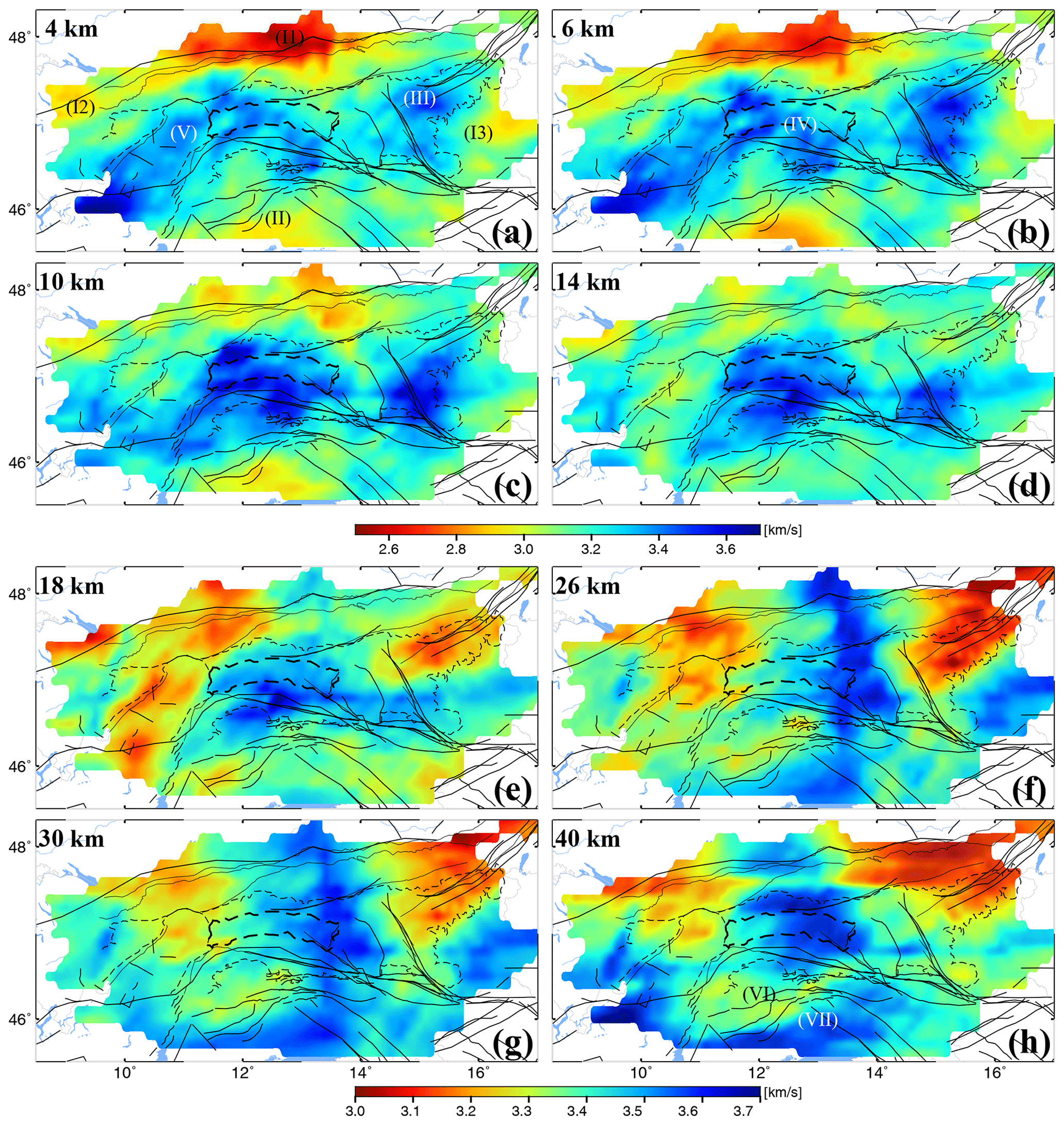
Figure 11 Shear velocity model derived from inversion of the Rayleigh-wave group velocity maps. Black lines represent the main faults in the region (modified from Schmid et al., 2004). Dashed lines show the main geological units of the region (geological map of the Eastern Alps, Egger et al., 1999; Fig. S4) to be compared with the velocity patterns, together with numbers indicating the geographical regions discussed in the “Results and discussion” section. See the text for the velocity anomalies marked by Roman numerals.

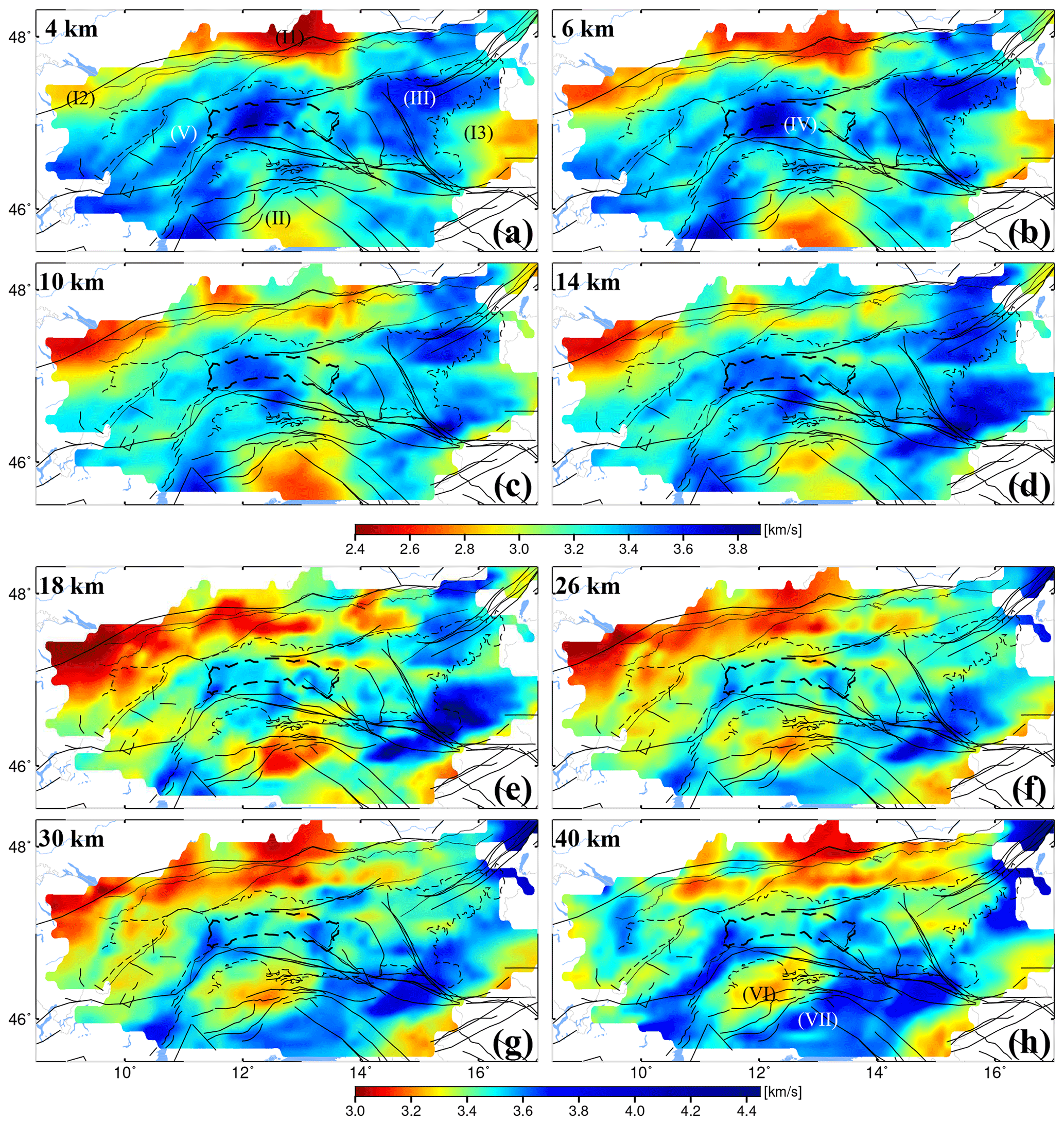
Figure 12 Shear velocity model derived from inversion of the Love-wave group velocity maps. Solid and dashed black lines are as in the previous figure. See the text for the velocity anomalies marked by Roman numerals.

6 Results and discussion

The shear velocity maps (Figs. 11 and  12) show a number of features that match surface geology and tectonic units. In the following sections we discuss several interesting features, first focusing on the upper crust and then on the lower crust. We will approach each feature by first discussing the constraints from the Rayleigh-wave Vs model (Fig. 11) and then the ones from the Love-wave Vs model (Fig. 12). To clarify the discussion, a simplified geologic map (Egger et al., 1999) is shown in Supplement Fig. S4.

6.1 Upper crust; correlation with geology

Similarly to the Rayleigh-wave group velocity maps, the Rayleigh-wave shear velocity (hereafter RVs) model (Fig. 11) shows a large high-velocity zone corresponding at the surface to basement units of the Tauern Window and Austroalpine units just north of the Periadriatic fault. The high-velocity area is bounded by two lower-velocity zones at all depth slices, which are associated with surface exposures of Mesozoic carbonates in the nappes of the Northern Calcareous Alps (NCA) and the Southern Alps (SA). The NCA corresponds to low shear velocities (< 3.1 km s⁻¹) down to 10 km of depth (Fig. 12). To the south, the velocity model clearly separates the SLA from the CZA. At 4 to 10 km of depth, the Dolomites of the Southern Alps show velocities of < 3.1 km s⁻¹. The northern margin of the SA (dashed line in Fig. 11a, b, c) clearly matches the boundary between high and low velocities. The same pattern is observed in the Love-wave shear velocity (hereafter LVs) model (Fig. 12).

A low-velocity anomaly (see the position labeled I1 in Figs. 11a and  12a) is found under the Molasse Basin, with velocities for basinal sediments ranging from 2.4 to 2.9 km s⁻¹. At depths of > 4 km, this low-velocity zone extends beneath the NCA in accordance with the occurrence of a south-dipping northern Alpine thrust fault that emplaced Mesozoic nappes of the NCA onto Neogene Molasse sediments (e.g., Brückl et al., 2010). The anomaly appears to extend down to 10 km of depth, indicating that the Neogene basinal sediments in the footwall of this fault form a wedge some 8–9 km thick (Steininger and Wessely, 2000; Hamilton et al., 2000). Alternatively, the anomaly extends no deeper than 8 km; the deeper part of this anomaly may be produced by downward smearing in connection with the prominent low velocity of the Molasse Basin. In the LVs model, the dominant low-velocity zones associated with the Molasse Basin (Fig. 12) extend down to about 8 km.

Another low-velocity anomaly in the northwestern part of the study area (labeled I2 in Figs. 11a and  12a) is more pronounced in the LVs model (Fig. 12). At shallow depths, it could be related to the Swiss Molasse Basin. Note that this anomaly is located at the edge of the study area where the ray coverage is relatively poor, particularly at longer periods. This leads to a decrease in the lateral resolution and the related Vs values. In addition, the low-velocity zone extends down to 20 to 22 km of depth, which may indicate a smearing effect with low velocity in the lower crust not necessarily reflecting the structures. A clear velocity contrast, labeled I3 in Figs. 11a and 12a, marks the eastern boarder of the CZA and the transition to the Styrian basin. However, this is also located at the edged of the study area, and care should be taken in interpreting this anomaly.

A low-velocity anomaly in the Southern Alps, labeled II in Fig. 11a and 12a, with values of less than 3 km s⁻¹ can be seen down to 10 km of depth beneath the Po Basin in northern Italy. This basin contains several kilometers of Mio-Pliocene clastic sediments derived from the retro-wedge of the Alps and the pro-wedge of the northern Apennines (Merlini et al., 2002). The Po Basin is also easily identified in the LVs model (Fig. 12) in which the velocity values and depth of the low-velocity zone are more or less as they are in the RVs model. Even though the low-velocity anomalies I2 and II match the location of the Swiss Molasse Basin and the Po Basin well, we should consider the fact that the anomalies are located at the edge of our study region with a lower ray-path density. This might affect the velocity values and the depth extent of the anomalies.

At the eastern part of the NCA, a small high-velocity anomaly (anomaly III; Figs. 11a and  12a) is observed at 4 and 6 km of depth in the RVs model. It shows up along the southern margin of the NCA and might be associated with the eastern greywacke zone, consisting primarily of Paleozoic low-grade metamorphic rocks. In the greywacke zone the model exhibits velocities of more than 3.5 km s⁻¹. Such high velocities are no longer visible at 10 km of depth. Similar high velocities have already been observed by Behm et al. (2016) between the SEMP fault and the northern Alpine thrust fault as well as towards the Bohemian Massif. They interpreted that feature as a southeastern tip of the Bohemian Massif dipping under the Alps. In the LVs model, this high-velocity zone is observed in a wider area. It can be traced down to 20 km of depth as the anomaly becomes smaller. Anomaly III extends south at 10 and 14 km of depth in RVs and becomes more prominent in LVs.

One of the most notable features of the shear-wave velocity model (anomaly IV; Figs. 11b and  12b) is the higher velocity in the western part of the Tauern Window compared to the eastern part. The velocity contrast in the TW is more visible in the LVs model (Fig. 11a, b, c). This anomaly is found at depths down to about 10 km in both RVs and LVs models. The TW exposes both Penninic basement and underlying Subpenninic units (Schmid et al., 2013), with the latter containing high-grade basement (Central Gneiss) of the Venediger complex exposed in two domes at the W and E ends of the TW (Fig. S1 Egger et al., 1999; Schmid et al., 2013). The western Tauern dome clearly corresponds to high velocities in our model. In contrast, the eastern Tauern dome exhibits lower velocities. The Central Gneiss is subdivided geologically into subunits such as Granatspitz in the west and the Hochalm nappes in the east (e.g., Frisch et al., 1998; Schmid et al., 2013). However, it is not yet clear how such different lithologies could produce different shear-wave velocity in the TW region.

The shear velocity models clearly illustrate the Silvretta and Ötztal–Bundschuh nappes (OTZ) to the west of the Tauern Window (anomaly V; Figs. 11a and  12a). These nappes are bounded by the Giudicarie fault and the Engadin Window at its eastern and western edges, as well as by the Inntal and Periadriatic faults at its northern and southern margins (see Fig. 1 for fault locations). Rocks of the Ötztal nappe underwent polymetamorphic metamorphism and deformation in Variscan and pre-Variscan time (e.g., Schuster et al., 2004). High shear velocity observed in this area might be associated with the Eoalpine high-grade metamorphic nappes, as seen in both the Rayleigh- and Love-wave shear velocity models. The high velocity related to the OTZ is observed down to 6 km of depth (Fig. 11b).

6.2 Lower crust

From depths 14–18 km downwards, we observe a clear separation between the high velocity under the TW and the low velocity beneath the OTZ. The high-velocity zone is cut by the Giudicarie fault, which sinistrally offsets the Periadriatic fault system (Fig. 11e). The Giudicarie fault can be traced down to 40 km, confirming that it affects almost the entire crust (e.g., Pomella et al., 2011, and references therein). However, the crust–mantle discontinuity (Moho) does not appear to be offset beneath the Giudicarie fault (Waldhauser et al., 2002; Spada et al., 2013), suggesting that this fault is a crustal feature that does not penetrate down to the mantle lithosphere.

Towards the south, the Periadriatic fault system (PAL) separates the Austroalpine nappes to the north from the Southern Alps, including the Dolomites, to the south (Schmid et al., 2004). In the upper crust down to a depth of 14 km, most of the high-velocity anomalies lie to the north of this fault. The PAL does not seem to separate units with different velocity structures. This may indicate that units with similar physical properties are located on either side of the fault.

The low velocity associated with the Neogene sediments of the Po Basin is quite clear at 4 and 6 km of depth. However, at 10 km and deeper, the velocity reduction appears to deepen northward and extend to the lower crust (marked VI in Fig. 12h). Since this feature is not located exactly under the Po Basin, it is unlikely that we have a smearing effect due to the dominant low velocity of the Po Basin. Such a smearing effect can also be ruled out because it cannot be observed at such depths away from the Po Basin. Beneath the Po Basin, a high-velocity zone at >22 km of depth can be seen in both the RVs model and the LVs model (marked VII in Figs. 11h and 12h). The margins of this high-velocity domain are marked with red lines in Fig. 13. They may show the boundary between intermediate and lower crust. More particularly, the southern margin might indicate the intermediate–lower crust boundary within the transition from thinned Dinaric crust to the Pannonian basin.

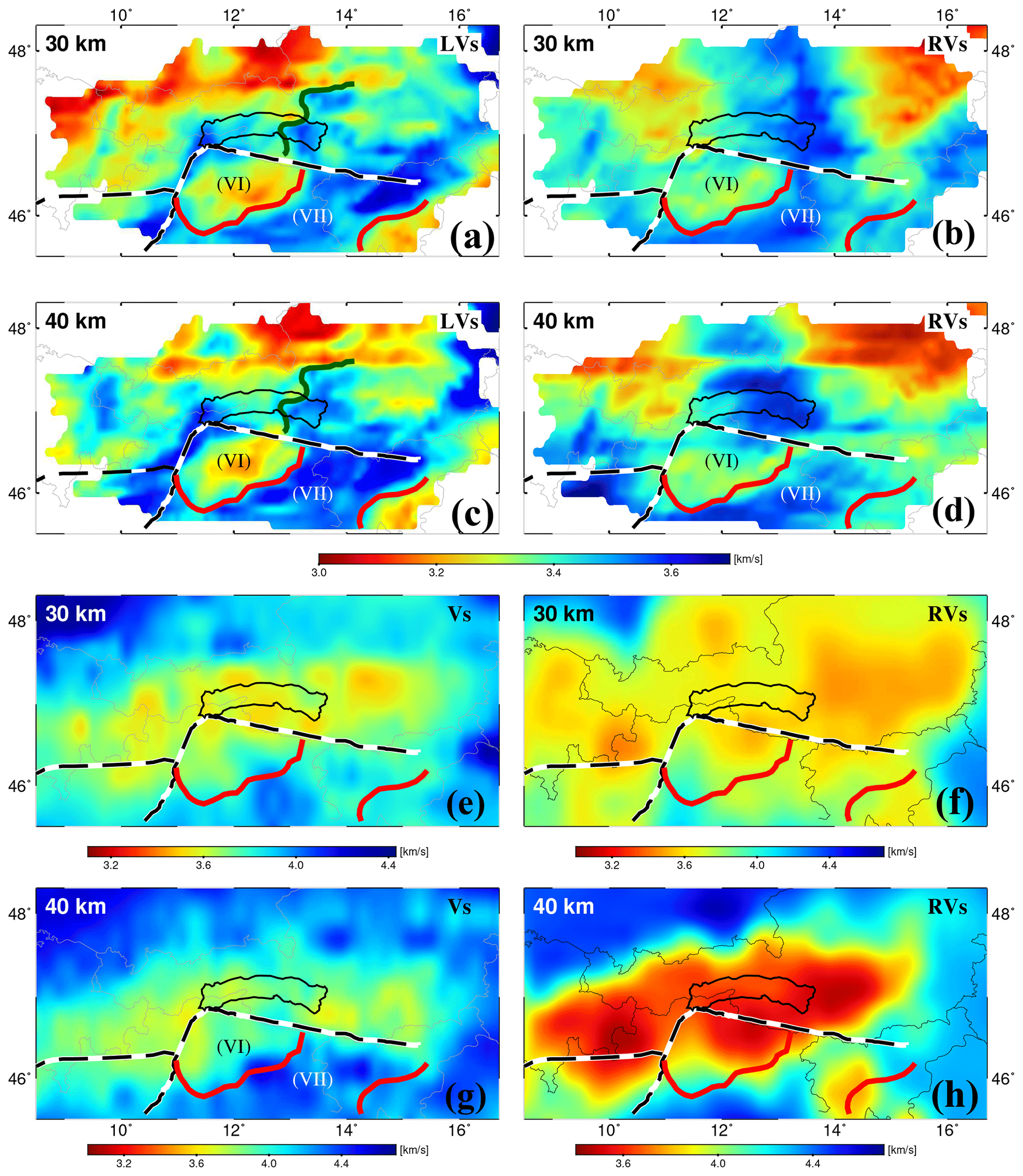
Figure 13 (a, c) Depth slices of the Love-wave shear velocity model (LVs). (b, d) The Rayleigh-wave Vs model (RVs) presented in this study. The red lines outline the high-velocity anomaly to the south of the Periadriatic line (PAL) marked by VII. Periadriatic and Giudicarie faults are shown as black and white lines labeled PL and GU in Fig. 1. The western margin of high velocity to the north of the PAL is marked by the dark green line. (e, g) Depth slices of the Vs model of Kästle et al. (2018) at 30 and 40 km of depth, respectively. (f, h) Depth slices of the RVs model of Lu et al. (2018) at 30 and 40 km of depth. The high-velocity anomaly marked VII in our Vs models can also be seen in the Kästle Vs model (e, g) and partly in the RVs of the Lu model (h).

In Fig. 13, we show depth slices at 30 and 40 km of our RVs and LVs models in comparison to the Vs model derived from surface-wave phase velocity using a combination of ambient noise and earthquake data (Kästle et al., 2018), as well as a Rayleigh-wave Vs model derived from ambient noise data (Lu et al., 2018). The anomaly VII observed at 30 and 40 km is marked by the red lines. It can also be observed at 30 and 40 km in Kästle et al. (2018), Fig. 13e and g. To the south of the PAL, the pattern of velocity changes in our model (Fig. 13a, b, c, d) and the Kästle model (Fig. 13e, g) are more or less similar; however, they do not show a similar pattern to the north of the PAL. Note that the Vs model of Kästle et al. (2018) has been derived jointly from Rayleigh and Love waves, while that presented here has separate Rayleigh-wave Vs and Love-wave Vs models. This could explain some discrepancies in the pattern of the anomalies between our models and Kästle et al. (2018) to the north of the PAL. Differences in station geometry could also be considered regarding some discrepancies between our model and Kästle et al. (2018). The anomaly VII can somehow be seen in Lu et al. (2018) in the 40 km depth slice (Fig. 13h). The relatively low-velocity anomaly VI, between the PAL and the anomaly VII (Fig. 12h), can also be observed in the Lu model (Fig. 13f, h). North of the PAL, our RVs model shows a low-velocity area at 30 and 40 km at the eastern part of the region. This can somewhat be seen in Lu et al. (2018) at 30 km. In addition, we see a clear high-velocity anomaly under the Tauern Window at 40 km of depth, while in Lu et al. (2018) we observe a broad low-velocity area at 40 km of depth. It seems that to the north of PAL where we have complex structures due to the interplay between orogen-normal shortening and orogen-parallel motion (e.g., Ratschbacher et al., 1991a), our models better resolve small-scale velocity contrasts and features.

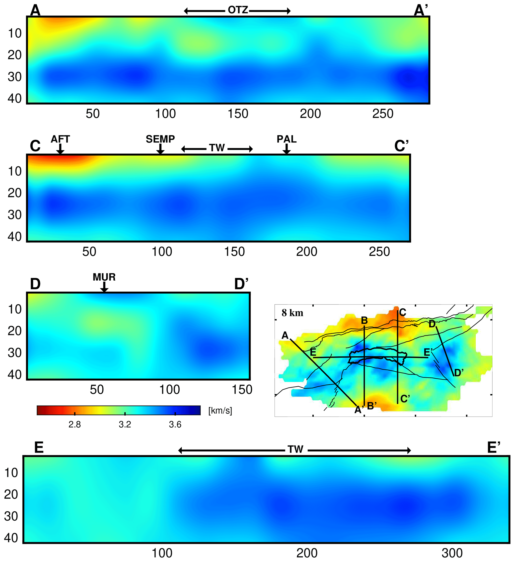
Figure 14 Cross sections of the Rayleigh-wave shear velocity model. Surface locations of the Ötztal block (OTZ), Tauern Window (TW), Periadriatic fault (PAL), Salzach–Ennstal–Mariazell–Puchberg (SEMP), northern Alpine Front Thrust (AFT), and Mur–Mürz fault (MUR) are shown on the profiles. Profile locations are presented in the 8 km depth slice. The Tauern Window (TW) and the main faults are shown by black lines (see Fig. 1 for fault names).

6.3 Cross-sectional view of the Vs model

Figure 14 shows cross sections of the RVs model presented in Fig. 11. Profile AA’ crosses the Austroalpine (Silvretta and Ötztal–Bundschuh) nappe system and the Giudicarie fault. The high velocity associated with the Silvretta and Ötztal–Bundschuh basement units is observed down to about 6 km of depth, and then a layer of lower-velocity anomaly can also be seen underneath this high-velocity anomaly. Profile CC' (Fig. 14) crosses the easternmost part of the TW. This profile at longitude 13.3^∘ E is roughly parallel to the EASI profile (AlpArray-EASI, 2014; Hetényi et al., 2018a). South of the Periadriatic fault in the Southern Alps, a velocity change at about 20–25 km of depth overlies the Moho depth at > 40 km (Behm et al., 2007a; Spada et al., 2013; Bianchi et al., 2015; Hetényi et al., 2018b). To the north of the TW and under the Molasse Basin, the velocity change is also observed, which may correspond to the boundary between the upper granitic and the lower mafic crust. Profile DD' (Fig. 14) crosses from the NCA across the Mur–Mürz fault to the Styrian basin. The high velocity in the vicinity of the Mur–Mürz fault in the uppermost 6 km seems to not be connected to any structure to the north. We also find a positive velocity change at about 10–15 km of depth along the southern part of the profile. The crust–mantle boundary (Moho) beneath this area is shallow (Behm et al., 2007a) and becomes shallower to the east, toward the Pannonian basin (Horváath et al., 2006). Previously, a crustal thinning was proposed for this area (Horváath et al., 2006, and previous studies). Behm et al. (2007b) also suggested a Moho jump of about 10 km under this area, which results in a Moho depth of 30 km. Such a sharp positive velocity change can be seen at 25–35 km of depth on the DD' profile, but it is not clear enough to be discussed with regards to a sharp change in the Moho depth along the profile. Profile EE' (Fig. 14) crosses the length of the Tauern Window from E to W. The high-velocity zone beneath the TW is probably associated with the European basement and can be tracked at depth eastward along the profile. A lower-velocity zone under part of the TW is also visible in the uppermost 15 km of depth on this profile.

Figure 15 shows profile BB'. It is oriented N–S, coincident with the TRANSALP profile (TRANSALP Working Group; Gebrande et al., 2002). Here the basement under the Tauern Window can be imaged as a high-velocity anomaly. A relatively low-velocity anomaly is observed beneath the Periadriatic fault zone at < 15 km of depth. A geological interpretation of the TRANSALP profile (Schmid et al., 2004; Bousquet et al., 2012) is also shown in Fig. 15. The pattern of the high-velocity zone associated with the sub-Tauern basement (marked with red dashed line) is in good agreement with the geological interpretation. A clear velocity contrast is observed at 20 km of depth under the Inntal fault and to the north. This could reflect the contrast between European upper crust and the lower crust. To the south of the Periadriatic fault, there is a south-dipping velocity contrast reaching 20 km of depth that cuts across the nappe contacts in the Southern Alps (Fig. 15). We speculate that this may correspond to a post-nappe metamorphic front that is below the current erosional level.

6.4 Effect of anisotropy

The shear velocity models extracted from Rayleigh and Love waves correlate well with most crustal geological and tectonic units down to 20 km. However, we observe some inconsistencies; for example, in the vicinity of the Mur–Mürz fault the LVs model shows higher shear velocity than the RVs model at most of the depths (Figs. 11, 12). Since we typically have very good ray coverage for both Rayleigh and Love waves at lower periods (meaning shallower depths) and therefore greater resolution, the difference between the Rayleigh and Love waves, especially in the uppermost 20 km of crust, is noteworthy. We have also assessed the possible effect of inversion parameters on the inverted velocity values and found that it has no significant effect on the inverted Rayleigh- and Love-wave velocities, more specifically on the Love–Rayleigh velocity ratio.

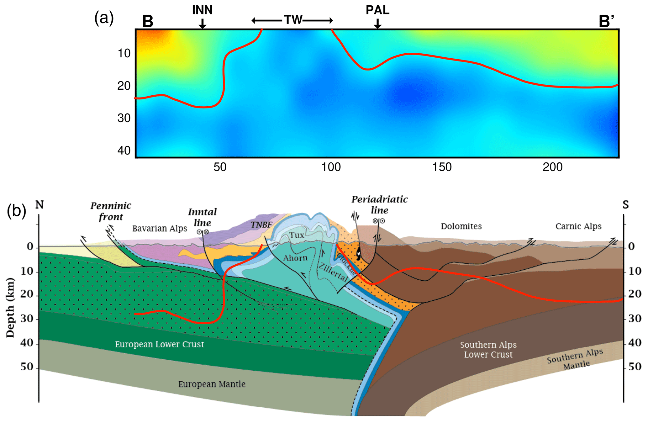
Figure 15 (a) Cross section of the RVs model along the TRANSALP profile. (b) Section showing geological interpretation of the TRANSALP in the surface location of the Tauern (Schmid et al., 2004; Bousquet et al., 2012). The red line in the Tauern Window area separates the high-velocity zone associated with the sub-Tauern basement from lower-velocity crustal rocks. South of this area, the line crosses nappe contacts in the Southern Alps. The Tauern Window (TW), Periadriatic fault (PAL), and Inntal line (INN) are shown on the profiles.

As Love and Rayleigh waves are sensitive to shear displacement in different orientations (horizontal versus vertical), different velocity anomalies between Rayleigh and Love, particularly high velocities of Love waves, may indicate seismic anisotropy. The observed velocity difference may be attributed to the preferred alignment of the main schistosity and shear zones subparallel to the shearing plane of the Mur–Mürz fault. The velocity difference between the western and the eastern parts of the Tauern Window (anomaly IV in Figs. 11 and 12) might be related to the difference in the orientations of the anisotropy. Structural data from deeply exhumed Penninic and Subpenninic units indicate that the main schistosity strikes NE–SW and is subvertical in upright, post-nappe folds of the west, whereas it is variably oriented to subhorizontal in folds in the east TW (Scharf et al., 2013; Rosenberg et al., 2018).

We also found a striking velocity difference in the RVs and LVs models to the east of the Tauern Window at > 20 km of depth (Fig. 12). This occurs in the eastwardly extruded block of orogenic crust (Alcapa) bounded by the aforementioned sinistral SEMP and dextral Periadriatic faults. Eastward, orogen-parallel escape of the Alcapa in Miocene time is attributed to a combination of indentation of the Adriatic Plate and pull in the upper plate of the retreating Carpathian orogen (e.g., Royden and Baldi, 1988; Ratschbacher et al., 1991a; Horváath et al., 2006; Favaro et al., 2017, and references therein). The velocity contrast at the western margin of the high-velocity domain (dark green line in Fig. 13a) is quite discordant to the trend of Moho depth contours (Spada et al., 2013) and might represent the boundary between thinned intermediate and lower crust of Alcapa. We interpret this velocity contrast as a possible zone of intracrustal decoupling at the base of the laterally eastward-extruded Alcapa unit. The observed velocity difference between the Love-wave Vs model and Rayleigh-wave model may reflect shear-induced anisotropy originating from eastward motion of the Alcapa block above the subducting lithosphere during Miocene Adria–Europe convergence. Such high velocity is not seen in the Kästle et al. (2018) Vs model, possibly due to the fact that their model is isotropic and jointly inverted from Rayleigh and Love dispersions. This inversion may have averaged any anisotropic effects due to contrasting Rayleigh–Love Vs differences. We do observe a slightly low-velocity anomaly to the east of the TW in the Rayleigh-wave model of Lu et al. (2018). Since they only presented a Rayleigh-wave Vs model, it is not possible to discuss and compare the anisotropy effect on the RVs and LVs difference from Lu et al. (2018).

However, here we have separately inverted Rayleigh and Love dispersions, which present well-resolved isotropic shear velocity models with observed Rayleigh and Love velocity inconsistency in some parts of the region. It may highlight a notable anisotropy signal, but we would need a joint inversion of Rayleigh and Love dispersions in order to build an anisotropic velocity model to confirm this observation.

7 Conclusions

We used 2 years of ambient noise data recorded at a set of permanent and temporary stations in the Eastern and Southern Alps with an average station spacing of 232 km in order to perform ambient noise tomography and to derive a local high-resolution Vs model of the crust. As an increment to the previously presented Vs model for the Alps (Kästle et al., 2018) and for Europe (Lu et al., 2018), we presented both Rayleigh-wave and Love-wave shear velocity models. Our high-resolution 3D shear velocity models show very good correlation between the velocity contrasts and geology projected to depth from the surface. The models reveal details of the crustal structure down to a depth of 40 km in higher resolutions that the previous Vs models (Kästle et al., 2018; Lu et al., 2018) have neither shown nor discussed.

The observed high-velocity anomalies are associated mainly with the crystalline core zone of the Alps, whereas the sediments of the Northern Calcareous Alps and the Southern Alps generally coincide with low velocities. The Molasse and Po Basin also correlate with low-velocity anomalies. Individual tectonic units (e.g., Silvretta and Ötztal–Bundschuh nappes, Koralpe unit) are also delimited by velocity contrasts. A velocity contrast at 20–25 km of depth found mainly south and north of the TW (profiles BB’ and CC'; Figs. 14, 15) perhaps represents a boundary between the upper and lower crust. The high velocity and velocity contrast observed at a depth > 20 km to the east of the TW can be interpreted as an intracrustal decoupling horizon that accommodated east-directed, orogen-parallel lateral extrusion of orogenic crust above lithospheric subduction during north–south Adria–Europe convergence.

Presenting separate Rayleigh- and Love-wave Vs models made us able to observe a number of discrepancies between the Rayleigh- and Love-wave shear velocities, e.g., around the Mur–Mürz fault that may be attributed to strain-induced orientation of the dominant foliation subparallel to the fault planes. Future studies of anisotropy are required to constrain the depth extent of this anisotropy, for example by jointly inverting the Rayleigh- and Love-wave dispersions to construct an anisotropic shear velocity model of the region.