Seismic waveform tomography of the central and eastern Mediterranean upper mantle

We present a seismic waveform tomography of the upper mantle beneath the central and eastern Mediterranean down to the mantle transition zone. Our methodology incorporates in a consistent manner the information from body and multimode surface waves, source effects, frequency dependence, wavefront healing, anisotropy and attenuation. This allows us to jointly image multiple parameters of the crust and upper mantle.

Based on the data from ∼ 17 000 unique source–receiver pairs, gathered from 80 earthquakes, we image radially anisotropic S velocity, P velocity and density. We use a multi-scale approach in which the longest periods (100–150 s) are inverted first, broadening to a period band of 28–150 s. Thanks to a strategy that combines long-period signals and a separation of body and surface wave signals, we are able to image down to the mantle transition zone in most of the model domain.

Our model shows considerable detail in especially the northern part of the domain, where data coverage is very dense, and displays a number of clear and coherent high-velocity structures across the domain that can be linked to episodes of current and past subduction. These include the Hellenic subduction zone, the Cyprus subduction zone and high-velocity anomalies beneath the Italian peninsula and the Dinarides. This model is able to explain data from new events that were not included in the inversion.

1 Introduction

Since the late 1970s (Dziewoński et al., 1977; Aki et al., 1977), seismic tomography has been emerging as the primary method for imaging the Earth's interior from the kilometre to the global scale. On regional to continental scales, the 3-D images can help to decipher the tectonic situation and history of an area by linking the surface observations to structures deeper in the mantle: high-velocity structures have been associated with subduction since the earliest days of seismic tomography.

The Mediterranean in particular is an area that has attracted much attention from the beginning – not in the least because of its strong seismicity and good data coverage. Classical ray tomography has been applied numerous times to study this area, both using body and surface waves (e.g. Spakman et al., 1988; Piromallo and Morelli, 1997, 2003; Amaru, 2007; Biryol et al., 2011; Koulakov et al., 2015; Portner et al., 2018; Snieder, 1988; Zielhuis and Nolet, 1994; Marone et al., 2004; Schivardi and Morelli, 2009; Salaün et al., 2012; Legendre et al., 2012).

As data availability increased, structures have thus been imaged with increasing amounts of detail. In the past, this has already led to hypotheses on the kinematics of the Mediterranean region that were testable against independent surface geological data (see, e.g. Wortel and Spakman, 2000; Faccenna et al., 2014). Nevertheless, ambiguities remain: in particular, the differences between body and surface wave studies can be striking, where surface wave anomalies are generally of larger amplitude but laterally smoother. Another difficulty is the connection between the crust and mantle, with most methods relying on some input crustal model whose accuracy may vary, depending on location (e.g. Bozdağ and Trampert, 2008; Laske et al., 2013; Fichtner et al., 2013c).

Continuing improvements in computing power have meanwhile facilitated the development of waveform tomography techniques (also referred to as full-waveform inversion or adjoint tomography) that allow us to fully account for the physics of wave propagation in 3-D heterogeneous media. By directly comparing observed seismograms with a simulated 3-D wavefield, a wealth of information can be extracted from the data. While computationally more expensive than ray-based imaging methods, the advantage of waveform methods lies in their ability to incorporate in a consistent manner all the information in seismograms – not just the arrivals of certain, specified phases. As a result, body and multimode surface waves, source effects, frequency dependence, wavefront healing, anisotropy and attenuation are naturally and coherently incorporated. The use of such a forward and inverse modelling technique largely excludes modelling artefacts in the imaging. Issues like the contamination of mantle structure that results from insufficient crustal corrections can thus be avoided (e.g. Montagner and Jobert, 1988; Bozdağ and Trampert, 2008). This makes waveform tomography especially suitable for imaging tectonically active parts of the Earth such as the Mediterranean, where large contrasts in elastic properties are likely to be present. It thus allows us to image S-wave and P-wave velocity jointly for the crust and mantle.

1.1 Objective and outline

In this study, we use waveform tomography to image the upper mantle beneath the central and eastern Mediterranean, inverting for the seismic velocities v_SH, v_SV and v_P as well as density ρ. Compared to the earlier, larger-scale European model of Fichtner et al. (2013c), our study provides a more local and zoomed-in model with clearer features that display stronger amplitudes. In the present study, we pay particular attention to developing a strategy that optimises the sensitivity to the deeper parts of the model domain by combining long-period surface wave data with a window selection strategy optimised for the selection of short-period body wave signals. This paper focuses on the technical construction of the model, discussing in detail the used methodology and the uncertainties and caveats of the methods and results. While we will highlight some key features of the resulting model, a detailed geological discussion will be the subject of a follow-up study.

After a brief introduction to the geological setting of the Mediterranean (Sect. 2), we will focus on the methodological aspects of the waveform tomography executed, discussing the model domain and data selection (Sect. 3) as well as the inversion setup (Sect. 4). The latter includes a description of the effects of window selection on the inversion. In Sect. 5, we discuss the main features of the resulting model, after which Sect. 6 is dedicated to validity tests of the model and a discussion of the limitations of the methodology.

2 Geological setting

Slow convergence between the African and Eurasian plates dominates the geological and tectonic setting of the Mediterranean domain (McKenzie, 1972; Dewey et al., 1989; Wortel and Spakman, 2000; Faccenna et al., 2014). This convergence (approximately 6 mm yr⁻¹; Reilinger et al., 2006) is currently mainly accommodated in the Alpine arc, the Hellenic arc and through complicated interactions between several plates and microplates present in the domain.

The Mediterranean is comprised of two basins of contrasting characteristics. The western Mediterranean consists of young oceanic lithosphere (∼30 Myr ago and younger; Wortel and Spakman, 2000) and the central/eastern Mediterranean is predominantly old (up to 340 Myr ago; Granot, 2016). This dichotomy is ultimately a result of the collision of the Adria plate (a promontory of the African plate) with the Eurasian crust at the location of the Alps – effectively cutting the basin in two (Channell, 1996; Faccenna et al., 2014). The young western Mediterranean formed during subsequent opening of the Liguro-Provençal and Tyrrhenian basins as a result of slab rollback (Faccenna et al., 2004). This rotated what is now the Italian peninsula to its current NW–SE orientation and resulted in the formation of the Apennines. It also brought Corsica and Sardinia from the Iberian Peninsula to their current locations and resulted in the steeply dipping Tyrrhenian subduction zone (e.g. Spakman and Wortel, 2004; Koulakov et al., 2015). The central/eastern Mediterranean, on the other hand, consists mainly of old African oceanic lithosphere – with the exception of the Aegean Sea, where current subduction beneath the Hellenic arc and slab rollback towards the southwest and south have resulted in a young extensional basin (e.g. McKenzie, 1978; Jolivet et al., 1994).

Several relatively large microplates play significant roles in the system (Fig. 1a). On the eastern end of the Mediterranean, the Arabian plate is moving northwards towards Eurasia along the Dead Sea Fault. West of the Arabian plate, the Anatolian microplate moves westwards relative to Eurasia and the Arabian plate. This is accommodated by the North Anatolian Fault and East Anatolian Fault. Continuing west, the Aegean microplate moves in a SW direction relative to Eurasia. The combination of these motions results in a anticlockwise rotation that has been attributed to the rollback of the Hellenic slab and effects of mantle convection and gravitational potential energy as a result of Anatolia's high elevation (Faccenna et al., 2014). Another subduction zone is visible beneath Cyprus, which some consider to be separated from the Hellenic subduction through the formation of a subduction-transform edge propagator (STEP) fault (Govers and Wortel, 2005; Özbakır et al., 2013).

3 Model domain and data

3.1 Choice of model domain

The chosen study area covers most of the central and eastern Mediterranean. This includes the tectonically interesting regions of the Italian peninsula, the Hellenic arc and Anatolia but also stretches towards the south to include the African coast (Fig. 1). In order to avoid artificial reflections from the boundaries when simulating wave propagation within this model domain, a buffer zone with absorbing boundaries is implemented (Cerjan et al., 1985).

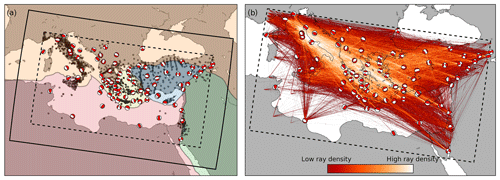
Figure 1 (a) The modelling domain in the central and eastern Mediterranean, with tectonic plates taken from Bird (2003): Africa in red, Eurasia in orange, Aegean plate in yellow, Anatolia in blue and the Arabian plate in green. Superimposed on top of this are the earthquakes used in this study (red–white focal mechanisms) and the locations of all seismic stations (black dots). A 3^∘ buffer zone separates the outer and inner model boundaries (solid and dashed lines, respectively). Within the buffer zone, wave propagation energy is absorbed that would otherwise result in artificial reflections. (b) An impression of “ray density” in the model domain, based on the great circle paths of all traces used in this study. This is just a rough proxy of coverage, serving only to highlight the variability and directionality of the coverage.

3.2 Data selection

The inversion is carried out using data from around 80 earthquakes that occurred within the model domain between 1998 and 2017 (Fig. 1a, Table S1 in the Supplement). Most of the tectonic activity is in the north of the model domain, so in order to obtain a coverage that is as homogeneous as possible, events are initially selected manually from the Incorporated Research Institutions for Seismology (IRIS) Searchable Product Depository (SPUD) moment tensor catalogue (http://ds.iris.edu/spud/momenttensor, last access: July 2019). Additional events are then obtained using automatic event selection from the Large-scale Seismic Inversion Framework package (LASIF; Krischer et al., 2015, http://lasif.net, last access: March 2020).

All moment tensors are taken from the Global CMT Project (Ekström et al., 2012; Dziewoński et al., 1981, https://www.globalcmt.org, last access: April 2020). Seismograms are downloaded automatically from the IRIS, ORFEUS, ETH, GFZ and KOERI data centres using the LASIF package. Since especially the depth and the moment tensor components linking horizontal and vertical motions can be poorly constrained when determined from long-period data (e.g. Kanamori and Given, 1981), we manually monitor the suitability of the earthquake data at all stages during the inversion. We excluded events that provided too few reliable measurements, e.g. because of cycle skipping or noise issues. In a few cases, we relocated or changed the timing of events where the (spatial) distribution of phase shifts indicated a clearly interpretable pattern (see Sect. S2 in the Supplement).

This approach results in around 80 events at the beginning of the inversion, corresponding to about 17 000 event–station pairs or 50 000 single-component channels, with a coverage that is excellent in the north but limited in the south (Fig. 1b). A table containing all earthquakes is available in Table S1.

4 Inversion setup

We perform regional waveform tomography by comparing the observed seismograms to synthetic seismograms, computed for subsequent iterations of model updates. Our inversion uses a deterministic, gradient-based iterative approach, such that the synthetic seismograms for consecutive models progressively provide a better match with the observed data. This optimisation method is local: updates are obtained by continuously moving in a direction of descent. There is therefore no guarantee that it will descend towards the global minimiser, i.e. the (set of) model(s) that would result in the lowest total misfit. The resulting model is therefore a function of several important strategies and choices, which are discussed below.

4.1 Seismic wave propagation

Synthetic seismograms are computed by simulating seismic wave propagation in 3-D within the model domain. Here, we solve the following wave equation:

$$\begin{array}{}\text{(1)}& \mathit{\rho }\left(\mathit{x}\right)\ddot{\mathit{u}}(\mathit{x},t)-\mathrm{\nabla }\cdot \mathit{\sigma }(\mathit{x},t)=\mathit{f}(\mathit{x},t),\end{array}$$

where ρ denotes density, u is the displacement field ($\ddot{\mathit{u}}$ being its second time derivative the acceleration field), σ the stress field and f the forcing term. We use the SES3D wave propagation code (Fichtner and Igel, 2008; Gokhberg and Fichtner, 2016) and invert for a rheology that includes radial anisotropy for S-wave velocity (SH and SV). Anelasticity, kept fixed, is implemented using memory variables (Blanch et al., 1995; Fichtner and van Driel, 2014). The rheology relates stress σ to displacement u. There are therefore four inverted parameters: the seismic wave speeds (v_SH, v_SV, and v_P) and density ρ.

4.2 Misfit definition

In order to quantify the differences between observed and synthetic waveforms, we use the time–frequency phase misfit functional of Fichtner et al. (2008):

$$\begin{array}{}\text{(2)}& \begin{array}{rl}& J_{\mathrm{TF},p}\left(\mathit{m}\right):=\\ & \underset{t}{\int }\underset{\mathit{\omega }}{\int }{W}_p^{\mathrm{2}}(t,\mathit{\omega }){\left[\mathit{\varphi }(\mathit{m},t,\mathit{\omega })-{\mathit{\varphi }}_{\mathrm{obs}}(t,\mathit{\omega })\right]}^{\mathrm{2}}\mathrm{d}t\mathrm{d}\mathit{\omega },\\ & W_p={\displaystyle \frac{\log (\mathrm{1}+|{\stackrel{\mathrm{̃}}{u}}_{\mathrm{obs}}\left|\right)}{\max \left(\log (\mathrm{1}+|{\stackrel{\mathrm{̃}}{u}}_{\mathrm{obs}}\left|\right)\right)}},\end{array}\end{array}$$

based on the phase shift (ϕ−ϕ_obs) for a given time window between observed and synthetic data from their time–frequency representations (calculated using the Gabor transform). A logarithmic time–frequency weighting function W_p determines the regions within that space that have sufficient amplitude such that meaningful measurements can be made, with $\stackrel{\mathrm{̃}}{u}$ being the time–frequency representation of seismic signal u as calculated via the Gabor transform. Misfits for all windows, traces and events are summed to produce the total misfit for a given model.

The advantage of this misfit definition is that it combines the sensitivity to phase shifts from, for instance, a cross-correlation time shift misfit (Luo and Schuster, 1991; Dahlen et al., 2000) and to the shape of waveforms from an L₂-norm misfit (e.g. Tarantola, 1984, 1986). It does not require the isolation of specific phases and is therefore specifically suitable for interfering phases. However, it is beneficial to isolate small- and large-amplitude signals in separate windows such that the information from small-amplitude signals is not suppressed by the weighting W_p (Sect. 4.6).

4.3 Optimisation algorithm

The objective functional in Eq. (2) is minimised such that the synthetic seismograms for each consecutive model provide a better match with the observed data than the previous. We use a conjugate-gradient scheme (Nocedal and Wright, 2006; Fletcher and Reeves, 1964) to compute model updates. This algorithm makes use of the gradient of the current iteration's misfit with respect to the model parameters and a recursive term based on the previous iteration's descent direction.

The misfit gradient is constructed from sensitivity kernels obtained using the adjoint method (e.g. Tarantola, 1988; Tromp et al., 2005; Fichtner et al., 2006; Fichtner, 2010). The raw gradients for each model parameter are preprocessed before a descent direction is computed in order to improve convergence properties of the gradients. Kernels for each event are clipped at the 99th percentile in order to avoid too-strong localisation of updates especially in the source region and then summed to produce the misfit gradient. The side and bottom edges are set to zero to remove potential boundary effects, and some smoothing is applied. This processing routine, fully described in Table S2, is based on experience from previous inversions and some initial experimentation. It is re-evaluated at several points during the inversion. The processed gradients are used to compute a descent direction using the conjugate-gradient scheme, and the step length is then determined using a quadratic interpolation between the current model and three test models made with steps of lengths of 5 %, 7 % and 10 % of the maximum gradient amplitude. The final model for an iteration is obtained from the computed descent direction and the step length thus obtained.

4.4 Choice of initial model

Because of the local nature of the gradient-based optimisation, the choice of initial model is of crucial importance: the closer the initial model is to the global minimiser, the more likely it is that it lies within the same “misfit valley”.

Fichtner et al. (2013c) constructed a model of the European crust and upper mantle (with an embedded higher resolution model of Anatolia; Fichtner et al., 2013b). These models were constructed using waveform tomography and already include considerable detail. The starting model for the current study is retrieved from these by way of the initial stages of the Collaborative Seismic Earth Model (Afanasiev et al., 2015; Fichtner et al., 2018), which combines the local models with a smoother background of S20RTS anomalies (Ritsema et al., 1999). The transition between these is smooth, owing to the efforts of Afanasiev et al. (2015) to combine regional seismic tomography models into a coherent and consistent global model. This gives a starting model with considerable detail in the northern parts of the model domain (resolution lengths of down to 25 km; see also Fig. 4 in Fichtner et al., 2013b) but only very smooth structures in the southern parts (Fig. 2).

The initial crust was implemented in the form of a velocity gradient, meaning that the initial model has no sharp crust–mantle discontinuity. This approach is widely used in regional- to global-scale tomography (e.g. Fichtner and Igel, 2008; French and Romanowicz, 2014), and it mostly serves two purposes. (1) The absence of a discontinuity facilitates the construction of a finite-element mesh, and in particular, it avoids the presence of very small elements that would require a very small numerical time step. (2) An initially smooth transition between crust and mantle allows the data to actually modify its sharpness, thereby avoiding artefacts that may result from an incorrect a priori implementation of the Mohorovičić discontinuity. Thus, in the final model, the velocity gradient from crust to mantle is as sharp as required by the data. These advantages are balanced by the disadvantage of somewhat limited interpretability of the final model in the sense that no sharp separation between crust and mantle exists.

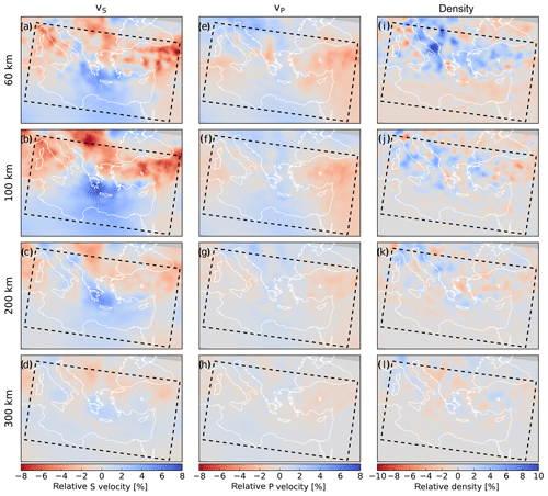
Figure 2 The starting model for (isotropic) S velocity, P velocity and density, as derived from Fichtner et al. (2013b, c). Slices are plotted at depths of 60, 100, 200 and 300 km, as relative deviations from the depth-averaged starting model. (a–d) Isotropic S velocity v_S, computed as the Voigt average of the anisotropic velocities v_SH and v_SV ($v_{\mathrm{S}}=\sqrt{\frac{\mathrm{1}}{\mathrm{3}}(v_{\mathrm{SH}}^{\mathrm{2}}+\mathrm{2}{v}_{\mathrm{SV}}^{\mathrm{2}})}$; e.g. Babuška and Cara, 1991), (e–h) P velocity v_P, (i–l) density ρ. Note the different colour scales.

4.5 Multi-scale approach

To further mitigate the risk of descending towards (insignificant) local minima, we use a multi-scale approach (Bunks et al., 1995). The lowest frequencies are inverted first, and as more of the data are explained by the model, higher frequencies are included in a stepwise manner. As a result of this approach, the large-scale structure within the model domain is obtained before small-scale details are filled in. This approach, a standard in waveform tomography (e.g. Akçelik et al., 2002; Tape et al., 2007; Virieux and Operto, 2009), mitigates the risk of cycle skips, spares computational resources and increases (at long periods) the proportion of the model domain that the data are sensitive to. This means that some of the long-wavelength structure of the southern, less-well-covered part of the model domain, can also be retrieved.

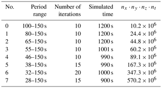
The used frequency bands are specified in Table 1. We start at long periods of 100–150 s to take full advantage of the comparatively minimal computational cost of such simulations and the broad sensitivity of such signals to almost the entire model space. Care is taken to avoid the introduction of cycle skips when new frequency content is introduced in the inversion. This is done by limiting the highest frequency to be less than 1.25 times the previous highest frequency. In each frequency band, ∼ 10–20 iterations are carried out.

At each frequency band, the events to be included are re-evaluated, mainly for the benefit of reducing computational cost (see Table 1). At low frequencies, events with few stations may provide valuable constraints on parts of the model domain that are otherwise poorly covered – several such events are located in northern Africa (Fig. 1). These events are mostly discarded at higher frequencies, where the benefit of including the event becomes unfavourable compared to the computational cost.

Table 1 Overview of inversion choices. Within each frequency band, ∼ 10–20 iterations are carried out, starting with the longest periods (Bunks et al., 1995). The “simulated time” column shows the duration of each synthetic earthquake simulation. As frequency increases, the surface wave train becomes more compact (see Fig. 3), so the simulation duration can be shortened. The final column $n_x\cdot n_y\cdot n_z\cdot n_t$ shows the product of the discretisation in the three spatial directions (number of elements) and time (number of time steps), which serves as an indication of the computational cost of a single forward simulation. This demonstrates that the bulk of the computational cost is in the final iterations; the first 50 iterations represent less than 25 % of the total computational cost.

In addition to the smoothing of the kernels as described in Sect. 4.3, we found it was necessary to apply additional processing to the total model update at the end of the iterations in some of the frequency bands. This mainly involved additional smoothing and removal of edge effects. All additional smoothing and damping is described in Table S2.

4.6 Waveform and window selection

For the initial three frequency bands (down to periods of 65 s), the first 1200 s of data after the event origin time were evaluated. This is reduced in subsequent period bands, where the surface wave train becomes more compact (see Fig. 3) and the computational cost per simulation increases (Table 1). Ideally, complete seismograms are used as data in the inversion. However, due to potential source- and receiver-side issues, geometry and noise, some selection of the data needs to be performed (Krischer et al., 2015). The initial window selection is carried out automatically using LASIF. For the first three frequency bands, windows are reviewed manually for all 50 000 seismograms; windows for later frequency bands are reviewed in part. During some initial experimentation, it was found that the inclusion of late arrivals could contribute to the formation of boundary artefacts, especially if the source or receiver are positioned close to the domain boundary. Such windows are therefore excluded.

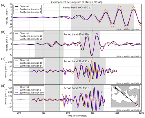
Figure 3 An illustration of the vertical-component seismogram recorded at MedNet station MN.AQU resulting from an earthquake in the Sinai region (27 June 2015, 15:34:03 UTC, M_w=5.6 – see inset) and corresponding synthetics for different period bands and iterations (see Table 1). Selected windows are shown as grey shaded areas. Vertical lines indicate P-wave (red) and S-wave (green) first arrival times predicted using the TauP toolkit (Crotwell et al., 1999) in ObsPy (Beyreuther et al., 2010) for PREM (Dziewoński and Anderson, 1981). In the final period band (d), we compare the initial model 0 with the final model. The fit of the body wave data improves visibly, but especially the fit of the surface wave train improves dramatically – this observation is typical for the entire dataset.

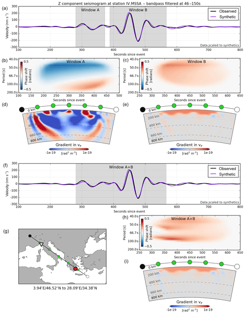
Figure 4 An illustration of the difference between selecting multiple windows or a single window in the presence of both small-amplitude and large-amplitude signals. (a) Observed and synthetic seismograms from an earthquake in the Aegean Sea (4 April 2014, 20:08:08 UTC, M_w=5.6), band-pass filtered between periods of 46 and 150 s, with two separate windows A and B. (b) Weighted time–frequency phase difference W_p(ϕ−ϕ_obs) (Eq. 2) between observed and synthetic seismograms for window A. (d) A cross section through the corresponding sensitivity kernel for v_P. (c, e) Phase difference and kernel for window B. Note that both kernels are on the same colour scale. Because window B is a surface wave window, it is to be expected that sensitivity to P velocity is much reduced. (f) The same traces as in panel (a) but now with a single combined window (A + B). (g) Map showing the location of the cross section, with the locations of the earthquake and station indicated by a red circle and yellow triangle, respectively. (h, i) Phase difference and kernel for the combined window (A + B). Note the similarity to the corresponding plots for window B (c, e) – a result of the weighting W_p that suppresses the effect of the small-amplitude signal.

Our window selection strategy is aimed to maximise sensitivity to deep structure. This is done by explicitly separating small- and large-amplitude signals into different windows, which allows us to make use of the (smaller-amplitude) body wave information. Figure 4 illustrates this. Two separate windows (A and B) reveal significant and complementary information in both wave packets, which is demonstrated by the deep sensitivity for v_P for body wave window A. In the combined window (A + B), both the misfit and the v_P sensitivity kernel are dominated by the large-amplitude surface wave signal, which is not significantly different from window B. Separating such windows accelerates the convergence of the body wave data and thus, given the finite total number iterations, allows us to better resolve deeper structure.

5 Results

A total of 100 conjugate-gradient model updates were calculated, divided over eight consecutive frequency bands going down to periods of 28 s (Table 1). In this section, we will discuss the resulting models and misfit development.

5.1 Misfit development

Figure 5 displays the misfit development for all the frequency bands used in this study. The misfit reduction varies per frequency band but is on the order of 10 %–20 % within each band.

Figure 5 Misfit development across iterations, normalised by the initial misfit within each frequency band. Within every frequency band, 10–20 conjugate-gradient updates are calculated (Table 1). In the period bands of 55–150 s and higher, windows were re-evaluated mid-period band, indicated with the label “Repick”. The increase in misfit at these points is a result of the fact that the objective functional is changed as additional windows are included – a result of the fact that the waveforms grow more similar. In some cases, the smoothing parameters (Sect. 4.3) are also changed mid-period band. This is done when the misfit development starts flattening out.

Comparing the initial and final models in the period band of 28–150 s, the misfit drops by 48 %. This is demonstrated in Figs. 6 and 7, where we compare observed traces for this period band with synthetics from the initial and final models using windows from the final iteration. Figure 6 demonstrates that the most important misfit improvements come from events clustering in the central Aegean part of the model domain and towards the southeast. The events with the largest initial misfit (which are the events with the largest number of windows) display the largest drop in misfit – both in absolute and in relative terms. Phase shifts per window become closer to zero for the final model.

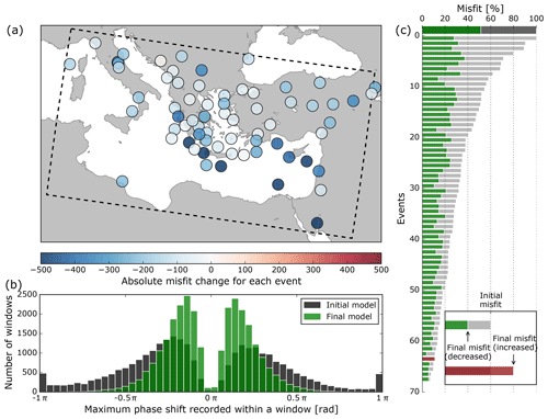
Figure 6 A comparison of the initial and final models in the shortest period band (28–150 s). (a) Geographical distribution of the absolute change in misfit for each of the events from the initial to the final model. (b) A comparison of maximum time–frequency phase shift between observed and synthetic seismograms within windows, for the initial (black) and final (green) models. A positive phase shift means that synthetics are ahead of observed data; a negative phase shift indicates the opposite. (c) Misfit for the initial (grey) and final (green/red) model, plotted both for the whole dataset (thick bar) and per event (narrow bars). Event values are scaled by the largest initial misfit and sorted by initial misfit. Total misfit decrease in this period band is 48 %. The strongest misfit decrease is generally seen for the events with the largest initial misfit. Note: the histograms in panel (b) contain a gap around zero phase shift as a result of the decision algorithm used to select or discard windows. This algorithm happens to include a criterion based on a division by the maximum absolute phase shift within a window. If the traces are very similar, this number is small and the resulting criterion big, resulting in rejection of the window. In other words, the window has a high risk of being (erroneously) rejected if the traces are very similar. The effect of this can be offset by slightly adapting the windows. As a result, however, the windows with a near-zero phase shift disappear from the distribution which consequently is very much non-Gaussian.

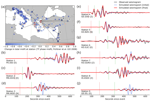
Figure 7 Misfit change for a single event and example seismograms. (a) Change in misfit for all stations of an event in the Aegean Sea (8 January 2013, 14:16:11 UTC, M_w=5.8), evaluated in period band 7 (28–150 s) (Table 1). Each dot represents the total change in misfit for a station. (b–j) Examples comparing observed (black) and synthetic seismograms for the indicated stations (initial model: dashed, pink; final model: red). Vertical lines indicate P-wave (red) and S-wave (green) arrival times predicted for PREM (Dziewoński and Anderson, 1981) using the TauP toolkit (Crotwell et al., 1999) in ObsPy (Beyreuther et al., 2010).

Figure 7 shows examples of seismogram fits for an event in the Aegean Sea. Especially at stations farther away from the source (e.g. stations 1 and 9), the difference between the synthetic seismograms for the initial and final models is striking.

5.2 Model

After 100 iterations, the model has been updated considerably for all parameters down to the transition zone (Fig. 8). Updates are strongest near the surface and decrease in strength with depth. P velocity is updated significantly less strongly than the other parameters and to shallower depths (Fig. 8a). Average shear velocities do not change significantly from the starting model (Fig. 8b), with average v_SH slightly higher than v_SV in the uppermost 100 km, as is reflected in the corresponding depth-averaged anisotropy $\frac{v_{\mathrm{SH}}-v_{\mathrm{SV}}}{v_{\mathrm{S}}}$ (Fig. 8c). Figure 9 shows how the Hellenic subduction zone becomes progressively more pronounced as iterations progress.

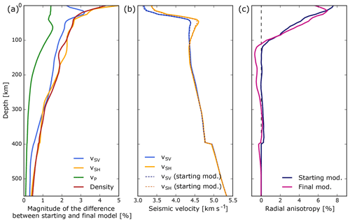
Figure 8 (a) Depth average of the magnitude of the relative difference between the initial and final models for all model parameters individually: $\mathrm{mean}\left(\right|({\mathit{m}}_f-{\mathit{m}}_i)/{\mathit{m}}_i\left|\right)$. (b) The depth-averaged horizontal and vertical shear wave velocities for the initial and final models. (c) Radial S anisotropy, given as $\frac{v_{\mathrm{SH}}-v_{\mathrm{SV}}}{v_{\mathrm{S}}}$.

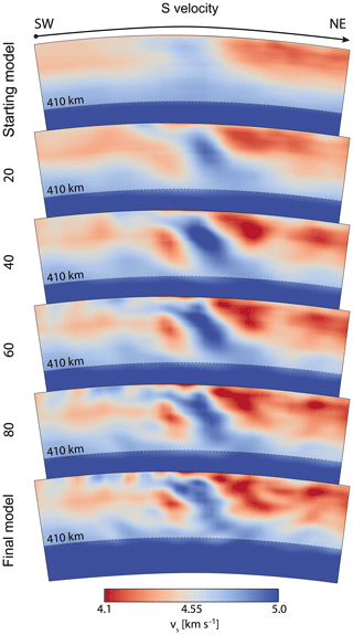
Figure 9 Development of the S-velocity model across iterations, in a southwest-to-northeast section that is perpendicular to the Hellenic subduction zone (see Fig. 1a). Plotted is the absolute isotropic S velocity v_S. The starting model (Fig. 2) is derived from Fichtner et al. (2013c). The section corresponds to the Hellenic section in Fig. 13d (dark green).

The final model is shown in Fig. 10 (compare to the starting model in Fig. 2). In general, the S-velocity model has features that can be linked most coherently with our knowledge of the geological situation. In the upper ∼100 km, the continental areas have slow velocities, while the old oceanic lithosphere of the central/eastern Mediterranean is fast. In contrast to this, both the western Mediterranean and the Aegean Sea display low velocities, as expected from their history of young oceanic crust formation and recent or ongoing extension. Several high-velocity zones can be linked to areas of known current or previous subduction. These will be discussed in more detail below.

The picture is not so clear for P velocity and density. P velocity has generally increased in the upper ∼200 km of the model domain, with smaller amplitudes than in S velocity. Because for a given frequency, wavelengths are longer for P waves, the resulting model is smoother than the S-velocity model. The Hellenic subduction zone is visible down to ∼250 km. At first sight, there appears to be an anticorrelation between P and S velocity; however, upon closer inspection, this turns out to be not actually the case – the P-wave model is fast in general. The density model, in contrast, has much shorter spatial wavelengths. This is a result of the fact that it is mainly contrasts in density to which the waves are sensitive. As a result, the imaged structures are of stronger amplitude and tend to be more oscillatory. Although this reaches greater depths (even beyond the transition zone), the results are much less coherent. We will discuss this separately below.

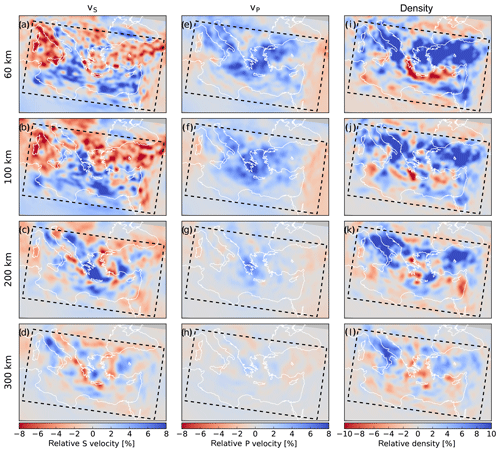
Figure 10 The final model for isotropic S velocity, P velocity and density – compare to Fig. 2. Slices are plotted at depths of 60, 100, 200 and 300 km, as relative deviations from the depth-averaged starting model. (a–d) Isotropic S velocity v_S, (e–h) P velocity v_P, (i–l) density. Note the different colour scales, where especially the amplitudes of variation in P velocity are much lower. Additional depth slices can be found in the Supplement.

The lateral variations of radial anisotropy, shown in Fig. 11, are dominated by structure with length scales of around 100–200 km. The maximum amplitudes of radial anisotropy reach nearly 15 %, already suggesting that intrinsic anisotropy (e.g. lattice-preferred orientation, or LPO, of olivine) is unlikely to be its only origin (Babuška and Cara, 1991). Other contributions include the strong differential sensitivity of Love and Rayleigh waves (Takeuchi and Saito, 1972) and apparent anisotropy induced by sub-wavelength structure that cannot be tomographically resolved (Backus, 1962). On the one hand, radial anisotropy is well known to be required in order to jointly explain Love- and Rayleigh-wave dispersion. On the other hand, it can be shown both analytically and numerically that the inherent (LPO related) and apparent anisotropy cannot be distinguished from seismological observations (Fichtner et al., 2013a; Wang et al., 2013). For the latter reason, we accept the required presence of radial anisotropy in our model but refrain from its geological interpretation.

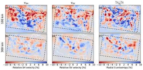
Figure 11 Anisotropy for the final model at 100 and 300 km depth. While anisotropy is required by the data in order to jointly explain Love- and Rayleigh-wave dispersion, interpretation of the anisotropy pattern is complicated by the differing sensitivities of Love and Rayleigh waves and the fact that it is not possible to separate intrinsic and extrinsic anisotropy (see main text).

High-velocity structures

Several distinct high-velocity structures are visible within the model. A 3-D rendering of these structures is shown in Fig. 12, visualised with the 4.75 km s⁻¹ velocity isosurface. This value is chosen because it is somewhat above the upper-mantle average and serves to emphasise the approximate outline of the high-velocity features. Cross sections are shown in Fig. 13.

Beneath Italy, a high-velocity body (labelled “A” in Fig. 12) stretches along most of the Italian peninsula underneath the Appenines towards Puglia and Sicily, visible between depths of ∼ 200–500 km (Fig. 13a, b). This structure, mostly clearly separated from the surface, is imaged in many other studies and is sometimes interpreted as the remains of Tethyan subduction or as delamination from the Italian peninsula (e.g. Piromallo and Morelli, 2003; Koulakov et al., 2015).

On the other side of the Adriatic sea, a high-velocity anomaly (labelled “B” in Fig. 12) stretches from the southern Dinarides south towards northern Greece. It is especially prominent underneath the southern Dinarides (Fig. 13b) but stretches along most of the Adriatic coast (Fig. 13c). In the north, an anomaly is only visible near the surface underneath the Adriatic sea (Fig. 13a). This Dinaric anomaly is imaged in other studies (e.g. Piromallo and Morelli, 2003; Amaru, 2007) and correlates with the location of geodetically inferred convergence and subduction of Adria beneath Eurasia (e.g. Bennett et al., 2008).

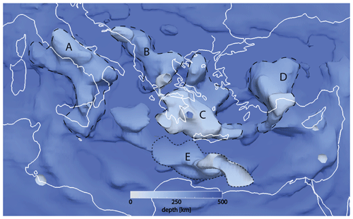
Figure 12 A 3-D rendering of high-velocity structures within the model domain. For this figure, the 4.75 km s⁻¹ isosurface of isotropic S velocity v_S was selected. This value is chosen because it is somewhat above the upper-mantle average and serves to emphasise the approximate outline of the high-velocity features. The model is coloured by depth, with shallower regions whiter and deeper regions bluer. The high velocities are labelled with letters: A: Italy/Appenines; B: Dinarides, C: Hellenic subduction zone, D: Anatolia. E is possibly an artefact. A 3-D visualisation video is available through the Supplement, as well as the vtk file for this figure – this can be viewed using, e.g. ParaView (Ahrens et al., 2005).

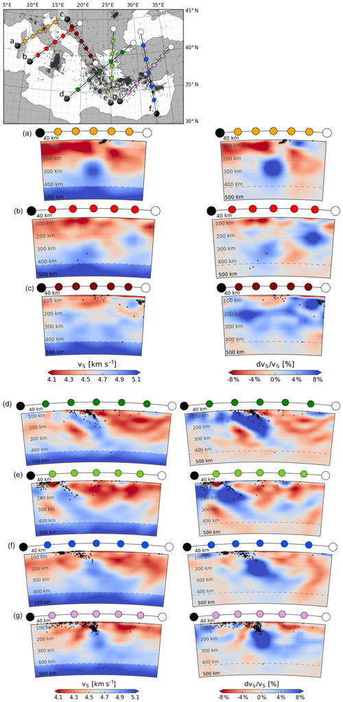
Figure 13 Cross sections through the S-velocity model and a map showing their locations. Left column: isotropic S velocity v_S; right column: relative deviations in v_S from the depth-averaged starting model. Black dots indicate seismicity in the region, as obtained from the European–Mediterranean Seismological Centre (EMSC-CSEM) catalogue (2004–August 2019, depths greater than 40 km and M>2;  Godey et al., 2013). Seismicity on the cross sections is plotted if it is within 50 km from the cross-section slice. Top: map showing the locations of the cross sections. (a) Cross section across northern Italy (anomaly A). (b) Cross section across Italy and the Dinarides (anomalies A and B). (c) Cross section parallel to the Dinaric anomaly (anomaly B). (d) Cross section across the Hellenic subduction zone (anomaly C). (e) Alternate orientation cross section of the Hellenic subduction zone (anomaly C). (f) Cross section across the Anatolian subduction zone (anomaly D). (g) Alternate cross section across the Anatolian subduction zone.

The most prominent and strongest high-velocity structure sits beneath the Hellenic arc and Aegean Sea (labelled “C” in Fig. 12) and has been widely interpreted as the African plate subducting beneath Eurasia. At the surface, it follows the curvature of the Hellenic arc from the Peloponnese towards Crete. The anomaly dips downward and inward in a northeasterly direction down to the top of the mantle transition zone (Fig. 13d, e). This structure has been imaged to various depths from the early days of seismic tomography and is generally believed to continue deep into the lower mantle (e.g. Spakman et al., 1988; Piromallo and Morelli, 1997; Amaru, 2007; Biryol et al., 2011; Portner et al., 2018; Hosseini, 2016). In our model, the fast anomaly flattens out towards the 410 km discontinuity and is not imaged in deeper parts (Fig. 13d, e). This is likely a result of a lack of sensitivity to depths beneath the mantle transition zone and should not be interpreted as an indication that the slab does not extend into the lower mantle.

Beneath western/central Anatolia, another high-velocity anomaly of large amplitude (labelled “D”) is visible, dipping northward from the Gulf of Antalya towards the transition zone (Fig. 13f, g). It is imaged in various other studies (e.g. Amaru, 2007; Biryol et al., 2011; Portner et al., 2018) and is interpreted as the deeper part of the Cyprian slab. In previous studies, the shallow part of this slab was imaged as near horizontal, stretching northward from the Cyprus trench (e.g. Bakırcı et al., 2012). At the surface, this part is thought by some to be separated from the Hellenic slab via the Pliny–Strabo STEP fault (Govers and Wortel, 2005; Özbakır et al., 2013), whereas others surmise the Pliny and Strabo faults to be part of a general African–Eurasian convergence system (Howell et al., 2017). In our images, this shallow part is imaged intermittently and a clear gap is visible between the shallow and deep parts of the slab, which extends into the transition zone (Fig. 13f, g).

A fifth anomaly, labelled “E”, is visible south of the Hellenic arc in Fig. 12. We will not interpret this further due to the poor data coverage in this area, mostly derived from a single earthquake.

In the Supplement, we further compare this model with model UU-P07 (Amaru, 2007).

6 Discussion

6.1 Advantages and limitations of the method and model

Although computationally more expensive than ray-based tomography methods, the advantage of waveform tomography lies in its ability to make use of all and any part of seismograms that has a sufficient signal-to-noise ratio, allowing for a more complete extraction of all information that is carried by seismic waves. This allows us to take into account body and multimode surface waves, source effects and frequency dependence, and jointly invert for multiple parameters for the crust and upper mantle. This is done in a manner where the misfit is computed directly from the observed and simulated seismograms, thus providing a self-consistent inversion framework. This method is particularly powerful in tectonically active parts of the Earth such as the Mediterranean, where strong heterogeneity is unavoidably present – circumstances under which the assumptions underlying ray theory become invalid.

Nevertheless, it is important to understand that the results are unavoidably affected by observational and methodological errors. In the following paragraphs, we will discuss some of these issues.

Moment tensors used in this inversion are taken from the Global Centroid Moment Tensor catalogue (Ekström et al., 2012) using the point source approximation. These are not inverted for separately, as limited azimuthal coverage – in particular, near the model domain boundaries – may lead to a bias in the results, as well as potential overfitting. Valentine and Woodhouse (2010) note that the model used for source inversions can have an imprint on tomographic results. Particularly in areas of limited coverage errors in the description of the source can have a large effect – this may be the case for anomaly E in Fig. 12. In order to minimise such effects, patterns in phase shift for each event are monitored manually and in some cases, source parameters were adjusted accordingly. In line with results from Bozdağ et al. (2016) and Hjörleifsdóttir and Ekström (2010), these adjustments are generally on the order of a few seconds or kilometres, and they correspond more closely to the reported International Seismological Centre (ISC-EHB) locations (Engdahl et al., 1998; Weston et al., 2018) as well as results reported in regional tectonic studies such as Howell et al. (2017). Examples are shown in Sect. S2. In a few cases, events were removed from the inversion altogether, as their waveforms showed a notable jump in complexity in the higher-frequency bands which may point to issues with the point source assumption or the source time function.

The wave propagation simulations are carried out on a regular mesh: a spherical chunk that includes no ellipticity, topography, ocean layer or explicitly meshed internal discontinuities. The neglect of topography can lead to small-scale artefacts near the surface, in particular if the topography is on the same length scale as the minimum wavelength (Nuber et al., 2016). Similarly, internal discontinuities and the effect of the water layer are not modelled explicitly. Especially near the surface, the model thus has to be interpreted as an effective representation of the real Earth, valid for the frequencies used in the inversion (Capdeville et al., 2010). Sharp or small-scale layering and (apparent) anisotropy thus cannot be distinguished reliably.

Another source of error is the actual data used in the inversion. Such errors can pertain to the location, orientation and timing of the receivers, as well as instrument errors and errors in the reported response. Many of these issues are caught using the automated quality control carried out in our workflow, but subtle errors remain difficult to catch. In areas of dense data coverage, this will average out, but in the regions of poor coverage, these may still affect the inverted result.

6.2 Fit to data not used in the inversion

Within the framework of the inversion and issues as outlined above, it is possible to analyse the trustworthiness (and limitations) of the model.

For this, we compute the misfit for the initial and final models for six earthquakes that were not part of the inversion (Table S1). We compare complete traces where no window selection has taken place in order to avoid preferential usage of data that “work well”. For this reason, and following Tape et al. (2010) and Simutė et al. (2016), we use for this a normalised L₂ waveform difference misfit:

$$\begin{array}{}\text{(3)}& J_{L_{\mathrm{2}}}={\displaystyle \frac{{\int }_t{\left[\mathit{u}(\mathit{m},t)-{\mathit{u}}_{\mathrm{obs}}\left(t\right)\right]}^{\mathrm{2}}\mathrm{d}t}{\sqrt{{\int }_t{\left[\mathit{u}(\mathit{m},t)\right]}^{\mathrm{2}}\mathrm{d}t{\int }_t{\left[{\mathit{u}}_{\mathrm{obs}}\left(t\right)\right]}^{\mathrm{2}}\mathrm{d}t}}}.\end{array}$$

Figure  shows the change in misfit for these events for all stations as well as example seismograms from events A–E (Table S1). The data fit improves both visually and quantitatively in the large majority of traces.

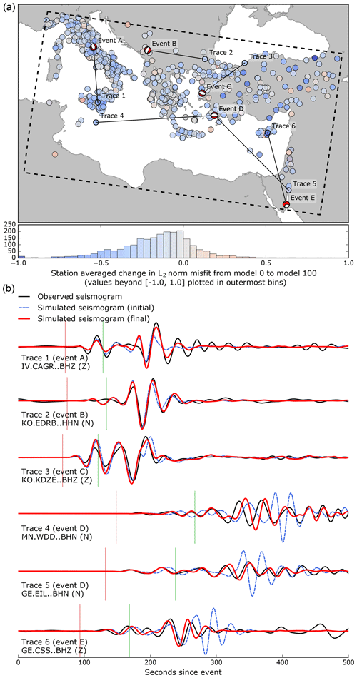
Figure 14 L₂ norm misfit decrease for new events and example traces. (a) Map with a dot representing the station-averaged change for each station in L₂ norm misfit for whole traces for all new events and a histogram with the same data. Misfit decreases for 79 % of the data. Total L₂ norm misfit decreases by 9 %, compared to 13 % for the original dataset. (b) Example seismograms showing observed data (black) compared with synthetics for the initial (dashed, pink) and final (red) models for the indicated source–receiver pairs.

6.3 Spike tests

In addition, we assess our model with what can be viewed as a “waveform tomography equivalent” for spike testing. While more sophisticated methods, such as resolution analysis through random probing (Fichtner and van Leeuwen, 2015) do exist, spike tests do not rely on any assumptions about the shape of point spread functions which – especially in the case of density – may be strongly non-Gaussian. They thus give qualitative insight into smearing in a way that is visually easy to interpret.

As Rawlinson and Spakman (2016) note, it is important in ray-theory travel-time tomography to use the ray paths of the actual model to assess recovery, smearing and trade-offs. To mimic this using the full wavefields computed from 3-D wave propagation, we add a grid of Gaussian anomalies onto one parameter in model 91 and use the real data to run five additional iterations in the final period band of 28–150 s. If the model is robust, the data will detect the (presumably) erroneous spikes, and updates will be generated that remove the anomalies. We do this for each parameter (v_SV, v_SH, v_P and density) individually, thereby also checking trade-offs. Spikes are introduced in an alternating chequered pattern at different depth levels.

In Fig. 14, we compare, at a depth of 100 km, the input anomaly (top row) with the part of the model update that is a result of the addition of the spikes (bottom four rows). This is computed by subtracting the reference model update (without spikes) from the update after five iterations of the spiked model: ${\mathit{u}}_{\mathrm{spike}}=({\mathit{m}}_{s+\mathrm{5}}-{\mathit{m}}_s)-({\mathit{m}}_{\mathrm{96}}-{\mathit{m}}_{\mathrm{91}})$.

Comparing Fig. 14 to Fig. 1, we immediately observe that those parts of the model domain that are well covered are indeed also the parts in which the spikes are most successfully removed. This is most visible for the first two rows, with spikes in v_SH and v_SV, respectively. These are also the parameters that are recovered best, with trade-offs to other parameters that are less significant. Recovery of v_P is, in general, very limited. Trade-offs from v_P to other parameters are partially stronger than the updates in v_P itself. This is in line with our observations of the final model (Sect. 5.2 and Fig. 10).

Recovery of density is also limited. Only in the central Aegean Sea is recovery of a level approaching that of v_SV and v_SH, and the negative spikes are surrounded by a positive “halo”. Furthermore, when comparing the different rows, we see that trade-offs to density from the other parameters are larger than the updates in density itself. While this is a test done over only a few iterations and it is possible that these trade-offs even out more as iterations progress, this does indicate that density is not a stable parameter.

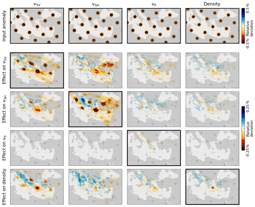
Figure 15 Spike tests conducted for model 91 in the period band 28–150 s, designed following the ideas of Rawlinson and Spakman (2016). Each of the columns represents a separate test with a chequered grid of spikes in one of the parameters. We denote the original model as m₉₁, the model with spikes as m_s and the model produced after five iterations as m_s+5. The updated reference model is m₉₆. The top row represents the input anomaly for that particular parameter, where we show m_o−m_s. In the following four rows, we show the cumulative model update after five iterations – i.e. $({\mathit{m}}_{s+\mathrm{5}}-{\mathit{m}}_s)-({\mathit{m}}_{\mathrm{96}}-{\mathit{m}}_{\mathrm{91}})$ – for each of the parameters. Results are shown for a depth of 100 km – additional slices can be found in the Supplement.

6.4 Perspectives on full-waveform inversion for density

The limited recovery of 3-D density structure is interesting in the context of previous numerical experiments, showing that density has a clear imprint on the seismic wavefield and may in principle be constrained (Płonka et al., 2016; Blom et al., 2017), especially at longer periods (Takeuchi and Saito, 1972). Furthermore, recent work in seismic exploration (e.g. Prieux et al., 2013; Operto and Miniussi, 2018; Pan et al., 2018) and regional seismology (e.g. Beller et al., 2017) has been encouraging.

The fact that density cannot be constrained reliably in the present study can be attributed to two main factors. Firstly, as density affects the seismic wavefield mainly through reflection/backscattering, it is predominantly contrasts in density that are imaged. This results in a sensitivity to density at much shorter length scales than for S velocity. It is therefore likely that short-scale structure from other parameters is mapped into density – this is especially likely near sharp transitions such as the surface and the Mohorovičić discontinuity, and may be exacerbated by the lack of topography/bathymetry and the ocean layer in our mesh. In the context of exploration seismology, indirect sensitivity to density through impedance contrasts can be exploited much more effectively through the use of reflected waves.

Furthermore, variations in density have a smaller effect on the seismic wavefield than variations in seismic velocity (Blom et al., 2017). This means that in the presence of noise, inaccuracies in the modelling method as discussed above, or variations in parameters not included explicitly in the inversion (e.g. attenuation or further anisotropy), density is likely to act as an “inversion garbage bin” (e.g. Operto and Miniussi, 2018; Pan et al., 2018). For this reason, we presently do not further interpret density, although it is still important to include this parameter in the inversion.

The way ahead in waveform inversion for density structure may require significantly more effort than we, admittedly, anticipated at the beginning of this study. Other physical parameters that are at a similar level of importance as density will need to be included in order to avoid that the neglect of one parameter pollutes the image of another. Likely candidates for such parameters are attenuation and more complex forms of anisotropy. An even larger number of model parameters will unavoidably decrease resolution of individual parameters and increase the influence of subjective regularisation, e.g. damping and smoothing. This subjective imprint can only be avoided by adopting a probabilistic approach to waveform inversion that only incorporates prior knowledge that we actually do have. The result would be a posterior distribution that reflects our honest state of knowledge on 3-D density in the Earth. Thanks to increasing computational resources and methodological advances, probabilistic full-waveform based on Monte Carlo sampling is starting to be within reach (e.g. Biswas and Sen, 2017; Gebraad et al., 2019).

7 Conclusions

We have imaged the upper mantle beneath the central and eastern Mediterranean using waveform tomography, simultaneously inverting for radially anisotropic S velocity, P velocity and density. We particularly aimed to resolve deep structure by using an approach that combines the use of long-period data at the beginning of the inversion with a windowing technique that optimally makes use of the separation of small-amplitude body waves from large-amplitude surface waves. This has resulted in a model in which several high-velocity structures are imaged down to the transition zone, which can be correlated to the current and past tectonic settings. This model is able to explain new data not used in the inversion.

Due to the natural dominance of surface wave signals in waveform tomography, our model is best constrained for S velocity, and we therefore base our interpretations on this parameter. P-wave velocity structure is less well recovered and smoother – a result of its longer wavelength for the same frequency – but broadly speaking it displays the same structures. Density, meanwhile, is poorly constrained, due to the sensitivity of the measurements to contrasts in density rather than the parameter itself, and due to the fact that of the imaged quantities, it has the smallest imprint on the wavefield, making it more sensitive to data or modelling errors. These observations are demonstrated using spike tests, and efforts are ongoing to improve the joint imaging of all parameters.

The Hellenic slab is the most prominent feature in the model. It extends from the surface down to the transition zone in a bent, arcuate shape. It is visible in both S and P velocity. Two more or less parallel anomalies are visible beneath the Italian peninsula and the Dinarides. The Italian anomaly is visible at depths below ∼100 km, whereas the Dinaric anomaly extends towards the surface beneath the southern Dinarides. Although extending towards Greece in the south, the Dinaridic anomaly is well separated from the Hellenic slab. The final large feature in the model is the high-velocity anomaly beneath Anatolia, interpreted as the Cyprus slab. This structure dips towards the north and east beneath the western and central parts of Anatolia. No clear connections between the shallow and dipping parts of the anomaly are imaged, and it is also well separated from the Hellenic slab.