the Creative Commons Attribution 4.0 License.
the Creative Commons Attribution 4.0 License.
 | 16 Jun 2021
Seismicity and seismotectonics of the Albstadt Shear Zone in the northern Alpine foreland
Sarah Mader
Joachim R. R. Ritter
Klaus Reicherter
The region around the town Albstadt, SW Germany, was struck by four damaging earthquakes with magnitudes greater than 5 during the last century. These earthquakes occurred along the Albstadt Shear Zone (ASZ), which is characterized by more or less continuous microseismicity. As there are no visible surface ruptures that may be connected to the fault zone, we study its characteristics by its seismicity distribution and faulting pattern. We use the earthquake data of the state earthquake service of Baden-Württemberg from 2011 to 2018 and complement it with additional phase picks beginning in 2016 at the AlpArray and StressTransfer seismic networks in the vicinity of the ASZ. This extended data set is used to determine new minimum 1-D seismic vp and vs velocity models and corresponding station delay times for earthquake relocation. Fault plane solutions are determined for selected events, and the principal stress directions are derived.
The minimum 1-D seismic velocity models have a simple and stable layering with increasing velocity with depth in the upper crust. The corresponding station delay times can be explained well by the lateral depth variation of the crystalline basement. The relocated events align about north–south with most of the seismic activity between the towns of Tübingen and Albstadt, east of the 9∘ E meridian. The events can be separated into several subclusters that indicate a segmentation of the ASZ. The majority of the 25 determined fault plane solutions feature an NNE–SSW strike but NNW–SSE-striking fault planes are also observed. The main fault plane associated with the ASZ dips steeply, and the rake indicates mainly sinistral strike-slip, but we also find minor components of normal and reverse faulting. The determined direction of the maximum horizontal stress of 140–149∘ is in good agreement with prior studies. Down to ca. 7–8 km depth is bigger than SV; below this depth, SV is the main stress component. The direction of indicates that the stress field in the area of the ASZ is mainly generated by the regional plate driving forces and the Alpine topography.
- Article
(7237 KB) - Full-text XML
-
Supplement
(1626 KB) - BibTeX
- EndNote


The Swabian Alb near the town of Albstadt (Fig. 1) is one of the most seismically active regions in Central Europe (Grünthal and the GSHAP Region 3 Working Group, 1999). In the last century, four earthquakes with magnitudes greater than 5 occurred in the region of the Albstadt Shear Zone (ASZ, Fig. 1, e.g., Stange and Brüstle, 2005; Leydecker, 2011). Today, such events could cause major damage, with economic costs amounting to several hundred million Euros (Tyagunov et al., 2006). Although the earthquakes caused major damage to buildings, such as fractures in walls and damaged roofs or chimneys, no surface ruptures have been found or described (e.g., Schneider, 1971). For this reason, the ASZ can only be analyzed by its seismicity to derive the geometry, possible segmentation and faulting pattern. One of the best observed earthquakes happened on 22 March 2003, and it was described as a sinistral strike-slip fault with a strike of 16∘ from north (Stange and Brüstle, 2005). This faulting mechanism is similar to the models of former major events (e.g., Schneider, 1973; Turnovsky, 1981; Kunze, 1982). In 2005, the seismic station network of the state earthquake service of Baden-Württemberg (LED) was changed and extended (Stange, 2018), and in summer 2015 the installation of the temporary Alp Array Seismic Network (AASN) started (Hetényi et al., 2018). In 2018 we started our project StressTransfer, in which we investigate areas of distinct seismicity in the northern Alpine foreland of southwestern Germany and the related stress field (Mader and Ritter, 2021). The StressTransfer network consist of 15 seismic stations, equipped with instruments of the KArlsruhe BroadBand Array (KABBA), in our research area (Fig. 1a).

Figure 1(a) Overview over our research area located in southwestern Germany in the northern Alpine foreland. The ASZ is our research target (framed area). Black triangles represent permanent seismic stations of the LED and other agencies. Yellow triangles represent temporary AlpArray seismic stations. Green triangles display the 15 temporary seismic stations of the StressTransfer network. The gray circles display the seismicity scaled by magnitude from 2011 to 2018. URG stands for Upper Rhine Graben. (b) Close-up of the area of the ASZ (framed area in (a)). Symbols are the same as in (a). The red-framed triangle highlights the central station Meßstetten (MSS) of the minimum 1-D seismic velocity model. White stars mark epicenters of the four strongest events, which had a magnitude greater than 5 in 1911, 2 in 1943 (same epicenter) and 1978, as well as the earthquake on 22 March 2003 with a local magnitude of 4.4 (Leydecker, 2011) these events are not included in the earthquake catalog from 2011 to 2018 (gray circles scaled with magnitude like in Fig. 1a). White lines indicate known and assumed faults (Regierungspräsidium Freiburg, 2019). The Hohenzollern Graben (HZG) is the only clear morphological feature in the close vicinity of the ASZ. Other large tectonic features are the Lauchert Graben (LG) and the Swabian Line (SL). Topography is based on the ETOPO1 Global Relief Model (Amante and Eakins, 2009; NOAA National Geophysical Data Center, 2009). (c) Overview on the geology of the research area region; geology data are taken from Asch (2005). Topography is based on SRTM15+ (Tozer et al., 2019).
Here we present a compilation of different data sets to refine hypocentral parameters of the ASZ. For this we analyze the earthquake catalog of the LED from 2011 to 2018 (Bulletin-Files des Landeserdbebendienstes B-W, 2018) and complement it with additional phase picks from recordings of AASN (AlpArray Seismic Network, 2015) and our own StressTransfer seismic stations. We calculate a new 1-D seismic velocity model and relocate the events. For several relocated events we calculate fault plane solutions. This procedure gives us a new view of the geometry of the fault pattern at depth in the ASZ based on its microseismic activity. Furthermore, we use the fault plane solutions to derive the orientation of the main stress components in the area of the ASZ and discuss these with known results.
Southwestern Germany is an area of low to moderate seismicity. The most active fault zones are the Upper Rhine Graben (URG) and the area of the ASZ and the Hohenzollern Graben system (HZG, Fig. 1b). In the region of the URG, the seismicity is distributed over a large area. In comparison, in our research area the seismicity clusters in the close area around the ASZ and the HZG.
The ASZ is named after the town of Albstadt, situated on the Swabian Alb, a mountain range in southern Germany (Fig. 1a). Southern Germany consists of several tectono-stratigraphic units, a polymetamorphic basement with a Mesozoic cover tilted towards southeast to east due to extension in the URG (Fig. 1c), associated with updoming (Reicherter et al., 2008; Meschede and Warr, 2019). The URG forms the western tectonic boundary, whereas the eastern boundary comprises the crystalline basement of the Bohemian Massif. To the south, the foreland basin of the Alps (Molasse Basin, Fig. 1c) frames the area in a triangular shape. The Molasse Basin covers the whole area south of the Swabian Alb up to the Alpine mountain chain. It is filled with Neogene terrestrial, freshwater and shallow marine sediments (Fig. 1c, Meschede and Warr, 2019). The Swabian Alb is bounded by the rivers Neckar in the north and Danube in the south (Fig. 1a). The sedimentary layers of the Swabian Alb, which consist of Jurassic limestone, marl, silt and clay, dip downwards by 4∘ to the southeast and disappear below the Molasse Basin (Fig. 1c) and the Alpine mountain chain (Meschede and Warr, 2019). The sedimentary cover of the Swabian Alb forms a typical cuesta landscape with major escarpments built up by resistant carbonates of the Late Jurassic that is cut by several large fault systems, which are detectable in the present-day topography (Reicherter et al., 2008). The Black Forest to the west of the Swabian Alb experienced the most extensive uplift due to the extension of the URG. Here, even metamorphic and magmatic rocks of the Paleozoic basement are exposed. To the north and northwest of the Swabian Alb, Triassic rocks crop out (Meschede and Warr, 2019). Due to the different uplift and erosional states of southern Germany, the depth of the crystalline basement varies strongly between −5.4 and 1.2 km a.s.l. (Rupf and Nitsch, 2008).
The current regional stress field of southwestern Germany is dominated by an average horizontal stress orientation of 150∘ (e.g., Müller et al., 1992; Plenefisch and Bonjer, 1997; Reinecker et al., 2010; Heidbach et al., 2016) and was determined from focal mechanism solutions, overcoring, borehole breakouts and hydraulic fracturing (e.g., Bonjer, 1997; Plenefisch and Bonjer, 1997; Kastrup et al., 2004; Reiter et al., 2015; Heidbach et al., 2016). It is characterized by NW–SE horizontal compression and NE–SW extension (e.g., Kastrup et al., 2004) and developed during late Miocene (Becker, 1993). Analysis of several kinematic indicators hint that fault planes where already activated repeatedly during the Cenozoic (Reicherter et al., 2008). Three main groups of fault planes can be observed. First, mainly sinistral NNE–SSW-to-N–S-striking fault planes, which are similar to the ASZ or the Lauchert Graben (Fig. 1b) and parallel the URG. Second, NW–SE-striking normal and/or dextral strike-slip fault planes, which correspond to the HZG in our area. Older kinematic indicators, like fiber tension gashes and stylolites, hint at a sinistral initiation of those NW–SE striking fault planes during the Late Cretaceous–Paleogene with a maximum horizontal compression in the NE–SW direction (Reicherter et al., 2008). Third, ENE–WSW-oriented fault planes, which are mainly inactive but with some exhibiting dextral strike-slip or reverse movement, for example, the Swabian Line (Schwäbisches Lineament, Fig. 1b). The direction of in our research area is quite constant, except of an area directly south of the HZG (Albstadt-Truchtelfingen) and within the HZG (Albstadt-Onstmettingen). There the direction rotates about 20∘ counterclockwise into the strike of the HZG (130∘, Baumann, 1986), which may be caused by a reduced marginal shear resistance.
The only morphologically visible tectonic feature close to Albstadt is the HZG (Fig. 1b), a small graben with an inversion of relief and a NW–SE strike (Schädel, 1976; Reinecker and Schneider, 2002). The 25 km long HZG has dip angles between 60–70∘ at the main faults and a maximum graben width of 1.5 km, which leads to a convergence depth of the main faults in 2–3 km depth (Schädel, 1976). Thus, the HZG is interpreted as a rather shallow tectonic feature. To the north and south of Albstadt there are further similar graben structures like the HZG, namely the Filder Graben, Rottenburg Flexure, western Lake Constance faults and Hegau, which are also about parallel to the main horizontal stress field (Reinecker et al., 2010) like the HZG. Reinecker and Schneider (2002) propose a tectonic model to relate the graben structures with the ASZ below. They apply the result of Tron and Brun (1991), who showed that the movement of a partly decoupled strike-slip fault in the subsurface can generate graben structures at the surface in a steplike arrangement. In the regional tectonic model, the graben structures are the HZG, the Rottenburg Flexure, western Lake Constance faults and the Filder Graben (Reinecker and Schneider, 2002). The ASZ itself is the strike-slip fault, partly decoupled from the surface by a layer of Middle Triassic evaporites in the overlying sedimentary layers (Reinecker and Schneider, 2002). Stange and Brüstle (2005) consider the bottom of the Mesozoic sediments a mechanical decoupling horizon as no earthquakes occur above 2 km depth.
Another tectonic feature in our research area is the ENE–WSW-striking Swabian Line north of the river Neckar (Fig. 1b). It extends from the Black Forest area partly parallel along the cuesta of the Swabian Alb to the east (Reicherter et al., 2008). The sense of movement along the Swabian Line is dextral. To the east of the ASZ near Sigmaringen, the Lauchert Graben strikes N–S, about parallel to the ASZ with a sinistral sense of displacement (Geyer and Gwinner, 2011, Fig. 1b).
The faults in southwestern Germany exhibit mainly moderate displacements during the last ca. 5 Myr (Reicherter et al., 2008). At the HZG, for example, the maximum vertical offset is of the order of 100–150 m. The horizontal offset is considerably lower and more difficult to determine (Reicherter et al., 2008).
Along the 9∘ E meridian Wetzel and Franzke (2003) identified a 5–10 km broad zone of lineations pursuable from Stuttgart to Lake Constance (Fig. 1a). Those lineations strike predominantly N–S, NW–SW and ENE–WSW. The N–S- and ENE–WSW-striking faults limited the NW–SE-striking graben structures like the HZG (Reicherter et al., 2008). The NW–SE-striking faults are expected to be possibly active at intersections with N–S-striking faults due to a reduction in shear resistance accompanied by aseismic creep (Schneider, 1979, 1993; Wetzel and Franzke, 2003).
The first documented earthquakes in the area of the ASZ occurred in 1655 near Tübingen and had an intensity of 7 to 7.5 (Leydecker, 2011). A similarly strong earthquake with a local magnitude of 6.1 occurred in 1911 near Albstadt-Ebingen (Fig. 1b, Leydecker, 2011), causing damage to buildings (Reicherter et al., 2008). The seismic shock triggered landslides with surface scarps in both the superficial Quaternary deposits and the Tertiary Molasse sediments (Sieberg and Lais, 1925) in the epicentral area and close to Lake Constance, demonstrating the potential of hazardous secondary earthquake effects (Reicherter et al., 2008). Since the 1911 earthquake, the Swabian Alb has been one of the most seismically active regions in the northern Alpine foreland, with a further three earthquakes with a local magnitude greater than 5 (Fig. 1b, 2 events in 1943, 1978, e.g., Reinecker and Schneider, 2002; Stange and Brüstle, 2005). The latest strong events occurred on 4 November 2019 (ML 3.8), 27 January 2020 (ML 3.5) and 1 December 2020 (ML 4.4, Regierungspräsidium Freiburg, 2020). The average seismic dislocation rates along the ASZ are on the order of 0.1 mm/a, respectively (Schneider, 1993). The return period of earthquakes along the ASZ with a magnitude of 5 is approximately 1000 years (Schneider, 1980; Reinecker and Schneider, 2002). Both estimates are based on historic earthquake records. From aftershock analyses and focal mechanism calculations we know that the ASZ is a steep NNE–SSW-oriented sinistral strike-slip fault (e.g., Haessler et al., 1980; Turnovsky, 1981; Stange and Brüstle, 2005) in the crystalline basement, as all earthquakes occur at a depth greater than 2 km (Stange and Brüstle, 2005). The lateral extent of the fault zone in an N–S direction is still under debate: Reinecker and Schneider (2002) propose an extension from northern Switzerland towards the north of Stuttgart, whereas Stange and Brüstle (2005) do not find this large extension as most of the seismicity happens on the Swabian Alb.
As a basis for our study, we use the earthquake catalog of the LED from 2011 to 2018 for earthquakes within the area close to the ASZ (8.5–9.5∘ E, 48–48.8∘ N, Fig. 1b). For these 575 earthquakes we received the bulletin files of the LED (Bulletin-Files des Landeserdbebendienstes, B-W, 2018), consisting of hypocenter location, origin time, local magnitude ML, and all phase travel time picks with corresponding quality and P-phase polarity. The LED picks from 2011 to 2018 are from 51 LED seismic stations and 14 seismic stations run by other agencies like the state earthquake service of Switzerland (Fig. 1a). Locations are determined with HYPOPLUS, a Hypoinverse variant modified following Oncescu et al. (1996), which allows the usage of a 1.5-D seismic velocity model approach (Stange and Brüstle, 2005). Most hypocenter depths are well determined, but around 9.7 % of the depth values are manually fixed. The median uncertainties for longitude, latitude and depth within the catalog are 0.5, 0.6 and 2.0 km, respectively. The magnitude ML ranges from 0.0 to 3.4, with average uncertainties of about ±0.2, and the magnitude of completeness is around ML 0.6 (see Fig. S1 in the Supplement). The catalog used only contains natural events, as quarry blasts are sorted out and induced events do not occur in the study region.
Additionally, within the AlpArray Project (Hetényi et al., 2018), nine seismic stations were installed starting in summer 2015 within 80 km distance to the ASZ, four of them directly around the ASZ (AlpArray Seismic Network, 2015, Fig. 1b). To get an even denser network and to detect microseismicity we started to install another 15 seismic broadband stations from the KABBA beginning in July 2018 in areas with striking seismicity in the northern Alpine foreland within our project StressTransfer (Fig. 1a) (Mader and Ritter, 2021). Five of those stations are located in the vicinity of the ASZ (Fig. 1b), and three of them where already running at the end of 2018.
We complemented the LED catalog with additional seismic P- and S-phase picks from the four AASN stations located around the ASZ from 2016 to 2018 and our StressTransfer stations recording in 2018. In total, our combined data set consists of 575 earthquakes (Fig. 1b) with 4521 direct P-phase and 4567 direct S-phase travel time picks from 69 seismic stations.
4.1 Phase picking
To complement the LED catalog, we use a self-written code in ObsPy (e.g., Beyreuther et al., 2010) for semi-automatic manual picking of the direct P and S phases. The raw waveform recordings are bandpass-filtered with a zero-phase four corners Butterworth filter from 3 to 15 Hz. Using the hypocenter coordinates of the LED we calculate an approximate arrival time at a seismic station. Around this arrival time, we define a noise and a signal time window following Diehl et al. (2012) so that we can calculate the signal to noise ratio (SNR) of our phase onsets. Our code automatically calculates the earliest possible pick (ep) and the latest possible pick (lp) (see Diehl et al., 2012) to get consistent error boundaries for each pick. Finally, the error boundaries are checked by eye, and the phase pick is done manually between the two error boundaries. The qualities of 0 up to 4 of the picked arrival time are set depending on the time difference between ep and lp (Table A1 in the Appendix). For consistency, a similar relationship is used between picking quality and uncertainty as defined by the LED (Bulletin-Files des Landeserdbebendienstes B-W, 2018).
4.2 Inversion for minimum 1-D seismic velocity models with VELEST
The LED uses the program HYPOPLUS (Oncescu et al., 1996) for routine location, with which one can apply a 1.5-D approach by using several 1-D seismic velocity models for selected regions (Stange and Brüstle, 2005; Bulletin-Files des Landeserdbebendienstes B-W, 2018). They use two P-wave velocity (vp) models, a Swabian Jura model and a model for the state of Baden-Württemberg, and they define the S-wave velocity (vs) model using a constant ratio (Stange and Brüstle, 2005; Bulletin-Files des Landeserdbebendienstes B-W, 2018, Fig. 4a, b). Furthermore, no station delay times are used (Bulletin-Files des Landeserdbebendienstes B-W, 2018).
To determine a complemented catalog, we invert for new minimum 1-D seismic vp and vs models in the region of the ASZ with station delay times, using the program VELEST (Kissling et al., 1994, 1995, VELEST Version 4.5). As central recording station we chose the station Meßstetten (MSS, Fig. 1b), as this station was running during our complete observational period and it is the oldest seismic recording site on the Swabian Alb, having been recording since 2 June 1933 (Hiller, 1933). To get the best subset of our catalog for the inversion, we select only events with at least eight P-arrival times for the inversion for vp and either eight P-arrival or eight S-arrival times for the simultaneous inversion for vp and vs. The P-pick times exhibit a quality of 1 or better, and the S-picks need a quality of 2 or better (Table A1). Events outside of the region of interest, 48.17–48.50∘ N and 8.75–9.15∘ E, with an azimuthal GAP greater than 150∘ and an epicentral distance of more than 80 km are rejected. This selection leads to a high-quality subset of 68 events with 789 P-phase picks for vp and 99 events with 945 P-picks and 1019 S-phase picks for the vp and vs inversion (Fig. 2).
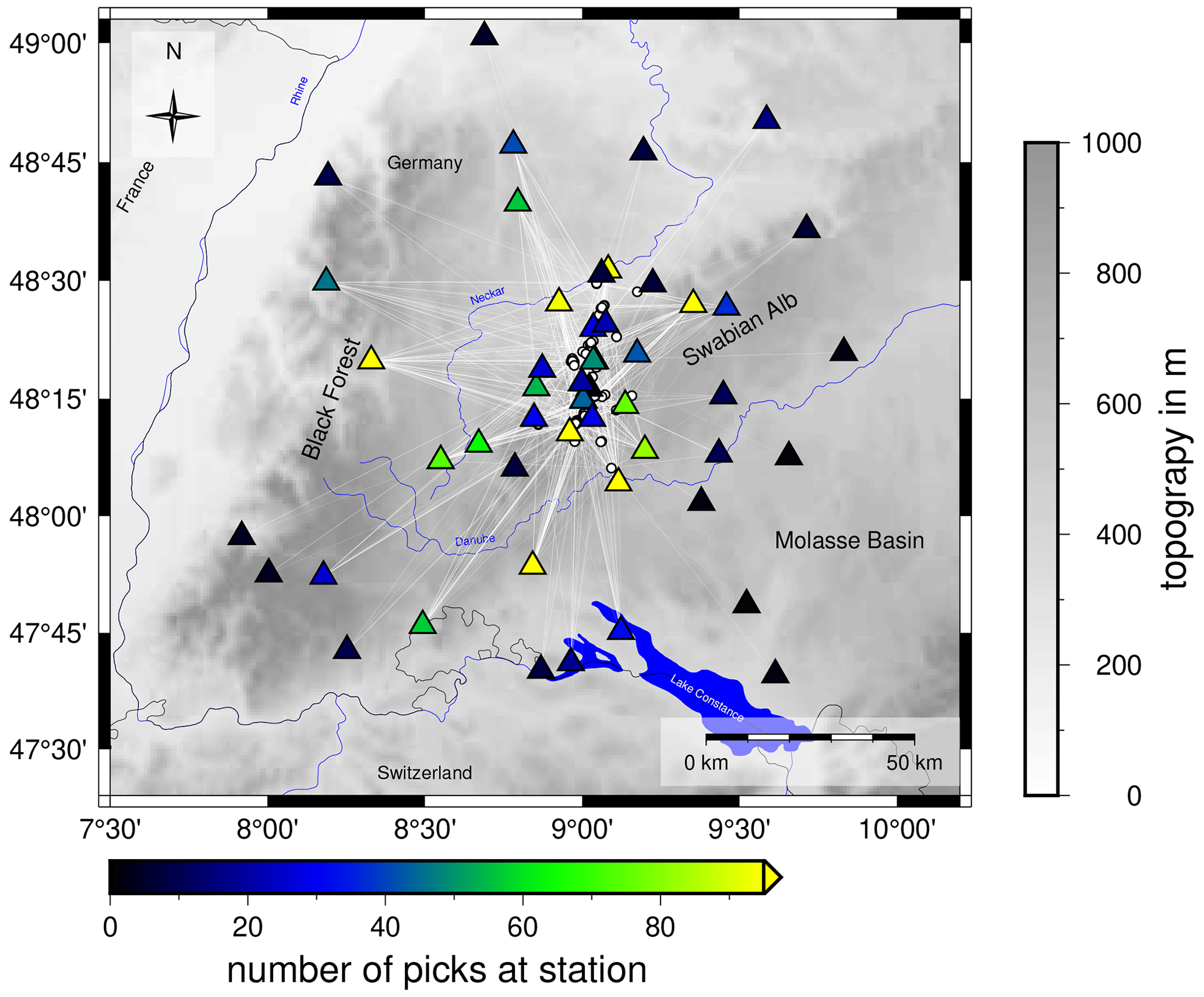
Figure 2Ray coverage and input data set for the inversion with VELEST. White circles represent the 99 selected events that are used for vp and vs inversion. Seismic stations are indicated as triangles and color-coded with the number of high-quality picks at a station used for the vp and vs inversion. Topography is based on the ETOPO1 Global Relief Model (Amante and Eakins, 2009; NOAA National Geophysical Data Center, 2009).
To probe our seismic velocity model space, inversions with 84 different starting models are calculated with four differently layered models from seismic refraction profile interpretations (Gajewski and Prodehl, 1985; Gajewski et al., 1987; Aichroth et al., 1992), the LED Swabian Jura model (Stange and Brüstle, 2005) and realistic random vp variations (Fig. 3). We apply a staggered inversion scheme following Kissling et al. (1995) and Gräber (1993), first inverting for vp and then for vp and vs together while damping the vp model. The inversion for vp was done with the 84 different starting models described previously, always using the resulting velocity model of the prior inversion as input for the next inversion with VELEST. After three to four inversion runs, the velocity models converged, and the results did not change (Fig. 3). Following this, the inversion for station delay times was done. The minimum 1-D vp model with the smallest rms and the simplest layering was selected as the final vp model for the simultaneous vp and vs inversion. Together with a ratio of 1.69 (Stange and Brüstle, 2005), it was also used to calculate the vs starting model, which was randomly changed to get a total of 21 vs starting models (Fig. 3). The inversion was done like the staggered inversion for vp. The resulting minimum 1-D vp and vs models (ASZmod1, Fig. 4) were selected due to their small rms.
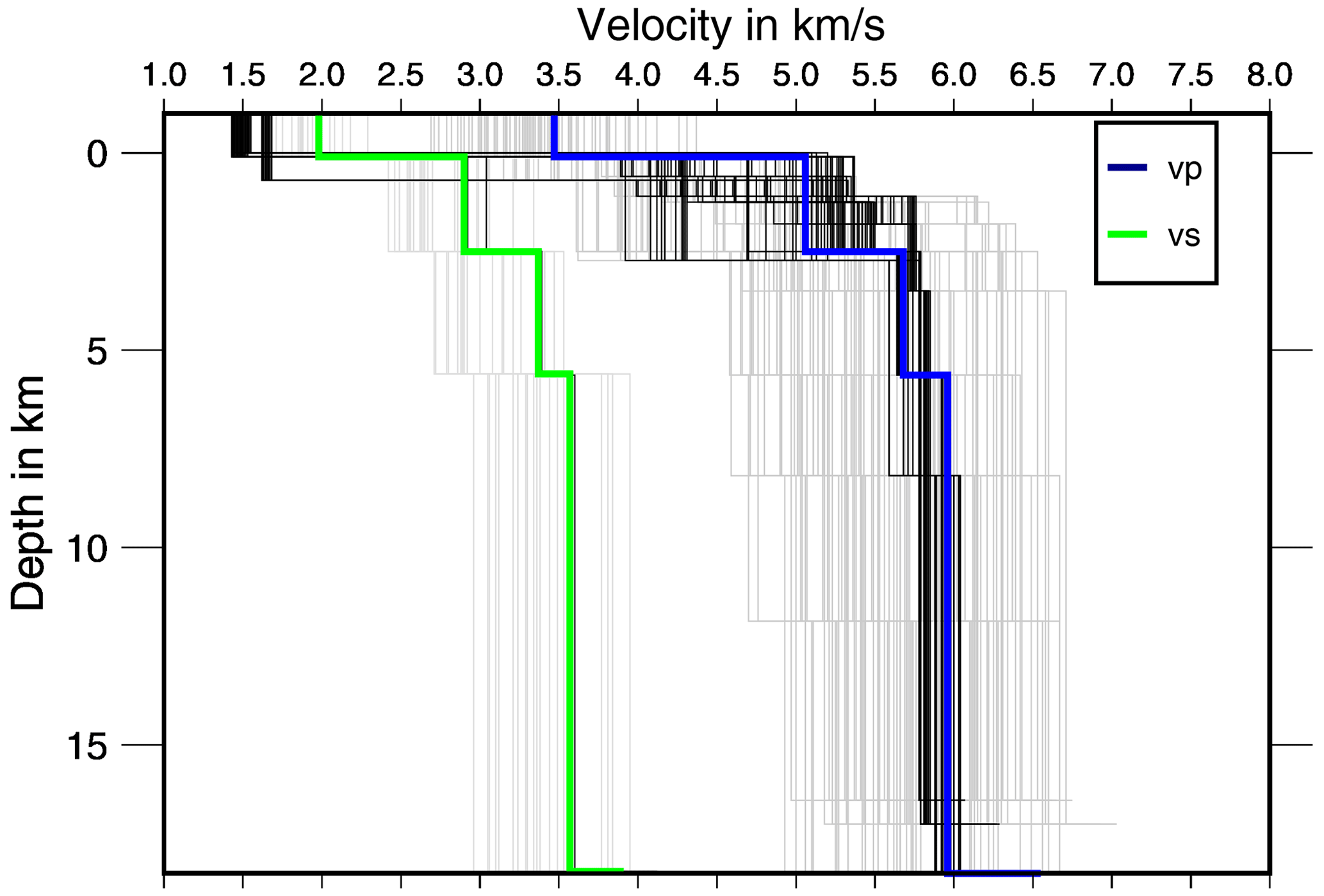
Figure 3VELEST input models for vp (84) and vs (21) (gray) and output vp (84) and vs (21) after inversion (black) together with the chosen model ASZmod1 (colored). A good convergence of the models can be observed, especially for vs. The second layer converges worst. An instability of the first layer with a tendency to unrealistic low seismic velocities can be seen. For this reason, the velocity of ASZmod1 was fixed in the first layer.
To test the stability of ASZmod1, we randomly shifted all 99 events in space by maximum 0.1∘ horizontally and 5 km with depth (Kissling et al., 1995). The result of this shift test demonstrates that we can determine stable hypocenters, with an average deviation of less than 0.005∘ horizontally and of less than 2 km in depth for more than 90 % of the events in the catalog (Fig. S2). The seismic velocities are stable, except for the first and second layer (Fig. S3a, b). The first layer was unstable already during the inversion process (Fig. 3); therefore, we damped its layer velocities and set them to realistic vp and vs values based on the seismic vp of the refraction profile interpretations (Gajewski et al., 1987). The instability in both upper layers may be caused by few refracting rays and thus small horizontal ray lengths through the layers. Furthermore, there are only a few earthquakes located within these layers (Fig. S3c). In total, the stability test (Figs. S2 and S3) indicates that the model represents the data and region very well and that the determined hypocenter locations are stable.
Table 1ASZmod1 with corresponding error estimates based on 2σ.
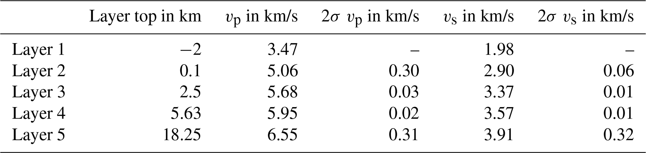
We calculated an error estimate based on the variation of the 21 output vp and vs models with our chosen layer model of Gajewski et al. (1987) for ASZmod1 (Table 1). For a precise estimation we determined 2 times the standard deviation (2σ) of the velocity models for each layer. For the uppermost layer we could not estimate any error, as the first layer was manually set and strongly damped during the inversion process. The 2σ range is small for the third and fourth layers. This was expected as most of the events are located within those layers and as all other models (which also have different layering) converge to similar velocities in those layers (Fig. 3). The error estimate for the second layer has to be considered carefully as this layer revealed strong instabilities during the stability test (Fig. S3). The fifth layer also has larger 2σ uncertainties relative to layers three and four, which is caused by less ray coverage and there being no events located below 18.25 km depth.
4.3 Relocation, station corrections and error estimation with NonLinLoc
To relocalize the complete earthquake catalog we use the program NonLinLoc (NLL, Lomax et al., 2000), a nonlinear oct-tree search algorithm. NLL calculates travel time tables following the eikonal finite-difference scheme of Podvin and Lecomte (1991) on a predefined grid, here using 1 km grid spacing. With the implemented oct-tree search algorithm, (density) plots of the probability density function (PDF) of each event are determined following the inversion approach of Tarantola and Valette (1982) with either the L2-rms likelihood function (L2) or the equal differential time likelihood function (EDT). The determined PDF contains location uncertainties due to phase arrival time errors, theoretical travel time estimation errors and the geometry of the network (Husen et al., 2003). Based on the PDFs an error ellipsoid (68 % confidence) is determined, which we use to calculate latitude, longitude and depth error estimates for each earthquake (Fig. 5). The estimated errors of our events (especially the depth error estimate) have been getting smaller since 2016. This reduction correlates well with the increased number of picks per event and thus with the increased number of seismic stations around the ASZ due to the modification of the LED network and the installation of the AASN and the StressTransfer stations from 2018 (Hetényi et al., 2018; Stange, 2018, Fig. 5). As a final hypocenter solution the maximum likelihood hypocenter is selected, which corresponds to the minimum of the PDF.
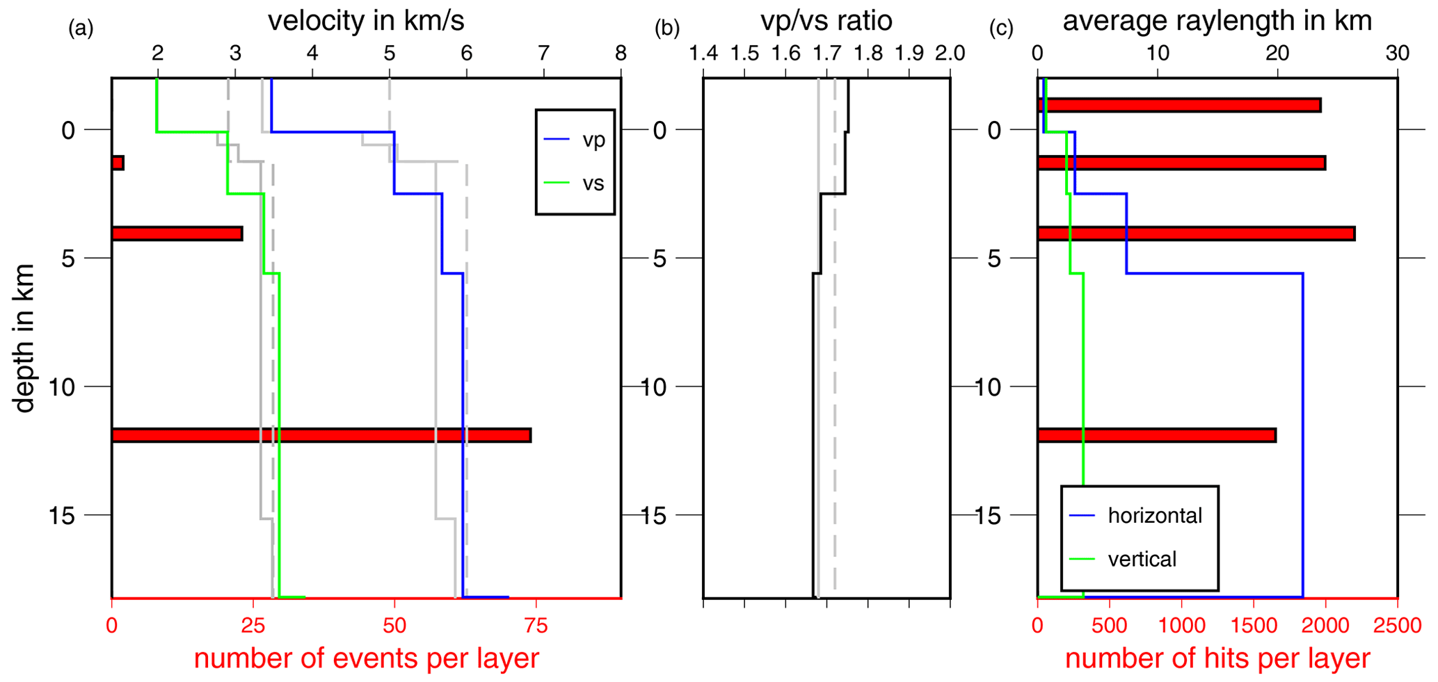
Figure 4(a) Final minimum 1-D seismic velocity models (ASZmod1): vs is in green, and vp is in blue. Gray lines represent velocity models of the LED (Bulletin-Files des Landeserdbebendienstes B-W, 2018): solid lines show Swabian Jura models, and dashed lines show Baden-Württemberg models. Red bars are scaled with the number of events in each layer of the velocity model. (b) ratio of ASZmod1 and the LED models. (c) Ray statistics of used ray paths. Red bars display number of hits per layer. Blue and green lines give the average horizontal and vertical ray length.
We compared the resulting hypocenters and error estimates using the L2 or the EDT likelihood function. The comparison mainly indicates similar earthquake locations, but we find EDT errors (Fig. S4) for many events that are too large and that are unrealistic (some greater than 50 km, leading to hypocenter shifts across the whole region). For this reason, we decided to use L2 for relocating our combined catalog.
In NLL one can examine station delay times calculated from the station residuals. The station delay times are defined as the time correction subtracted from the observed P- and S-wave arrival times. This implies that negative station delay times exhibit faster velocities relative to ASZmod1 and positive station delay times exhibit slower velocities relative to ASZmod1. We used ASZmod1 and the corresponding VELEST station delay times, as well as our high-quality subset of 99 earthquakes, as input for NLL. After four iterative runs of NLL, always using the output station delay times as new input station delay times, the determined station delay times become stable. As we want to relocate the whole catalog with NLL, we use the NLL updated VELEST station delay times for consistency. Since ASZmod1 is a 1-D seismic velocity model below the reference station MSS, we expect the station delay times to become zero for MSS. After four iterative runs the actually determined station delay times of MSS are 0.014 s with σ of 0.083 s for vp and −0.027 s with σ of 0.064 s for vs. As σ is bigger than the actual station delay time and the station delay time of MSS is smaller than the maximum error range of 0.05 s of our best determined picks (Quality 0, Table A1), we consider the station delay times of MSS to be practically zero. To account for similar small station delay times and σ, we state that all station delay times in the range of −0.05 to 0.05 s are practically zero station delay times if σ is greater than the actual station delay time (Fig. 6). The fact that the NLL station delay times of MSS and surrounding stations are close to zero indicates that even though they use a different (and nonlinear) relocation algorithm for delay time estimation than VELEST, our determined minimum 1-D seismic velocity model ASZmod1 represents the seismic velocity structure below MSS and its surroundings very well.
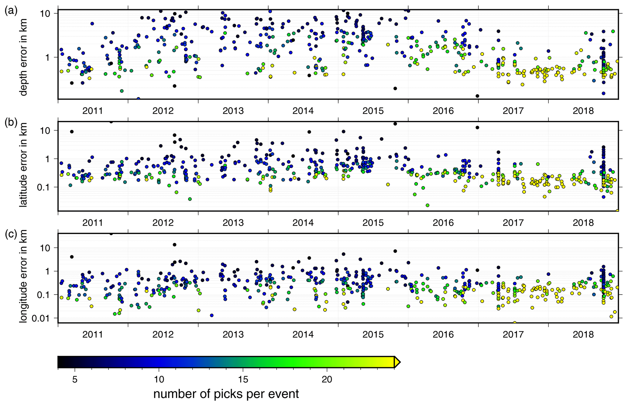
Figure 5Errors calculated from the 68 % confidence ellipsoid from NLL with L2 (L2-rms likelihood function) for each event in the combined catalog for (a) depth, (b) latitude and (c) longitude. The errors are color-coded depending on the number of picks, with dark colors indicating fewer picks and bright colors indicating many picks. Hypocenters with many observations are determined with smaller errors in depth and lateral position.
We compared the relocated catalog with the original LED locations. Some events have large differences in hypocenter coordinates (> 0.1∘ in latitude or longitude), which we identified as events with only a few arrival time picks (fewer than nine picks), a large azimuthal GAP (GAP > 180∘) or wrong phase picks. Furthermore, a large deviation of expectation and maximum likelihood hypocenters indicates an ill-conditioned inverse problem with a probable non-Gaussian distribution of the PDF (Lomax et al., 2000), which was the case for some events with only a few picked arrival times. Similar problems were also identified by Husen et al. (2003), who compared NLL locations with the routine locations of the state earthquake service of Switzerland. They also found that a good depth estimate with NLL depends on the station's distance from the earthquake. Especially for events with many observations, the depth estimate was worse if the closest station was further away than the focal depth of the event (Husen et al., 2003).
Our well-located earthquakes are selected by the following criteria: more than eight travel time picks, a GAP less than 180∘, a horizontal error estimate of less than 1 km and a depth error estimate of less than 2 km (Fig. 7). Some of our well-located events have quite different depth estimates compared to the LED solution (Fig. S5). Thus, we checked the station distribution for those events as proposed by Husen et al. (2003) and looked for incorrect phase picks. Nevertheless, all of these events have good phase picks, a small depth error estimate, evenly distributed stations and small deviations of expectation and maximum likelihood hypocenter coordinates. For this reason, we consider our new depth locations well determined and reliable.
In comparison with the LED catalog, the majority of our relocated earthquakes are characterized by a small eastward shift and a stronger clustering, especially in depth (Fig. S5). The latter may result from the hand-set depth location for some events of the LED.
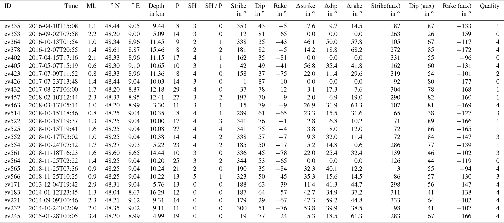
Table 2Parameters of the FOCMEC solutions. Values with (aux) refer to the assumed auxiliary plane.
4.4 Focal mechanism models with FOCMEC
We determine fault plane solutions for 25 selected events with the program FOCMEC (Snoke, 2003), which conducts a grid search over the complete focal sphere and outputs all possible fault plane solutions. For this we used the P-polarity picks of the LED (Bulletin-Files des Landeserdbebendienstes B-W, 2018), and for events since 2016 we added P and SH polarities, as well as SH P amplitude ratios, at the four AASN and three StressTransfer seismic stations. The local magnitude ML of those 25 events is in the range 0.6 to 3.4 (Table 2, Fig. 7, Bulletin-Files des Landeserdbebendienstes B-W, 2018).
To determine the SH P amplitude ratios we only used SH- or P-picks with a quality of 2 or better and the SNR of the picked phase needed to be greater than 5. Furthermore, we compared the frequency content of the P and SH phase to assure that the waves have the same damping properties, and the the source process was simple (Snoke, 2003). If the determined frequency of P and SH phases differed by more than 5 Hz the SH P amplitude ratio was omitted. All waveforms are instrument-corrected and bandpass-filtered between 1 and 25 Hz. As FOCMEC uses the ratio on the focal sphere we need to correct our amplitudes for attenuation effects and phase conversion effects at the free surface (Snoke, 2003). To correct for attenuation effects we use QP and QS values determined by Akinci et al. (2004) for southern Germany. The measured phase amplitude A depends on Q, the frequency of the phase f, the travel time t and the amplitude A0 at the source (e.g., Aki and Richards, 1980):
The correction factor for the free surface effect of SH waves is always 2 and independent of the incidence angle of the seismic wave. For the P wave the free surface correction strongly depends on the incidence angle and the ratio (e.g., Aki and Richards, 1980). We calculated the incidence angle for our P phases of interest with the TAUP package of ObsPy (e.g., Beyreuther et al., 2010) using the AK135 model (Kennett et al., 1995) and find incidence angles in a range between 22.9 and 23.2∘. As the variation between the incidence angles for the different station event combinations is very small, we use for all events the median incidence angle of 23.05∘. To calculate the ratio, we use vp and vs of the second layer of our model ASZmod1 (Table 1) because in the first layer the velocities are considered to be unstable. After this correction the logarithm of the SH P amplitude ratio is used as input in FOCMEC together with the P and SH polarities.
To find the appropriate solution one can allow different types of errors in FOCMEC. We compare the relative weighting mode and the unity weighting mode of the FOCMEC inversion for all events. This is done to explore if the results differ significantly, which could mean that they are questionable (Snoke, 2003). In the unity weighting mode each wrong polarity in the FOCMEC solution counts as an error of 1. In the relative weighting mode, polarity errors near a nodal plane count less than polarity errors in the middle of a quadrant. Thus, the polarity errors are weighted with respect to their distance to the nodal planes. This means an incorrect polarity is weighted by the calculated absolute value of the radiation factor (ranging between 0 and 1). For both weighting modes we searched for a solution. This is done by varying and systematically increasing the different possible errors. Those errors are uncertainties in the P and SH polarities and the total error of wrong SH P amplitude ratios, as well as the error range in which they are expected to be correct. For example, we might consider the unity weighting mode and an event with P and SH polarities. First, we check if we achieve a solution with zero errors for both. If no solution is found, we increase the allowed errors for the SH polarities to 1, as the SH-polarities are more insecure than the P polarities. If still no solution is found, we check for a wrong P-polarity and without wrong SH-polarity. This procedure is done for unity weighting and relative weighting, and it is stopped if a solution is found. To check for a dependency of the result on a single polarity, the next inversion runs for more errors are also determined.
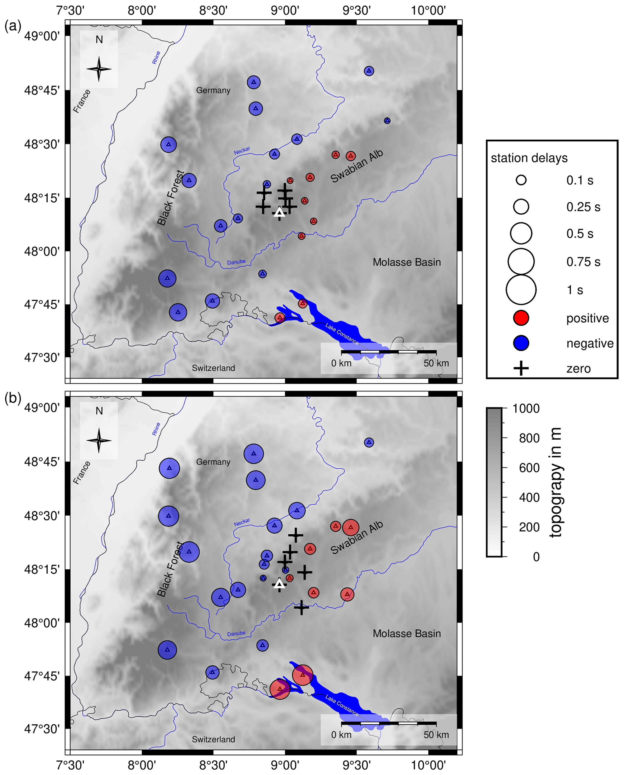
Figure 6(a) Station delay times for the vp velocity model ASZmod1. (b) Station delay times for the vs velocity model ASZmod1. Blue circles represent negative station delay times, indicating areas with faster velocities than ASZmod1. Red circles illustrate positive station delay times, indicating slower velocities than ASZmod1. Crosses are stations with zero station delays. Only stations with more than five travel time picks are included. The small white triangle highlights reference station MSS. Topography is based on the ETOPO1 Global Relief Model (Amante and Eakins, 2009; NOAA National Geophysical Data Center, 2009).
The output of FOCMEC results in a set of possible strike, dip, and rake combinations for each event. The fault plane solution closest to the medians of strike, dip and rake was chosen as the preferred solution (Table 2, Fig. S6). We use the other possible solutions to determine uncertainties for our preferred fault plane solution. For this we recalculate all strikes into a range between 90 and 270∘ to exclude large differences in strike by the transition from 360∘ back to 0∘ and by the 180∘ ambiguity of the strike. We determine the 5 % and 95 % percentiles of strike, dip and rake and calculate the width of the 5 % to 95 % percentile range (Δstrike, Δdip, Δrake, Table 2). These widths are taken as uncertainty ranges to account for a non-uniform solution distribution and to assign a quality factor to the determined fault plane solutions (Tables A2, 2). To get rid of non-unique or problematic cases the following restrictions are used: the median of the strike and dip of the unity and relative weighting modes has to be within a range of 15∘, the median of the rake must be within , and the total allowed number of solutions is limited to 500. Furthermore, if the solutions yield a quality of 4 with Δstrike, Δdip or Δrake greater than 75∘, the fault plane solutions is omitted. Finally, all remaining fault plane solutions are inspected manually.
We observe a low quality (3 and 4), especially for low-magnitude events (ML < 1.4) and events without SH polarities and SH P ratios (Table 2). In Fig. 7 the fault plane solutions are displayed scaled with magnitude and their individual event ID.
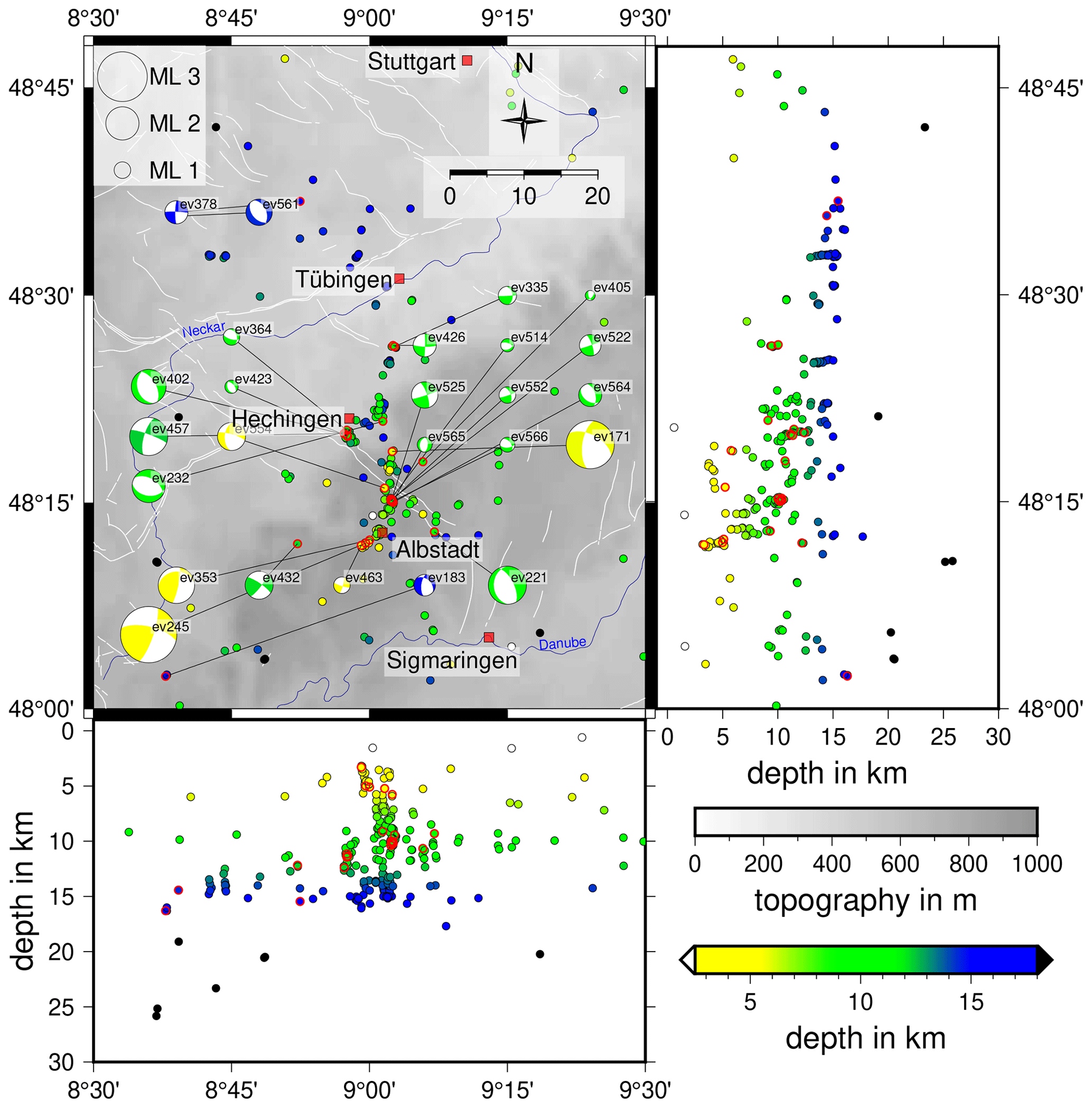
Figure 7Hypocenters of the 337 best-located events with a horizontal error of less than 1 km and a depth error of less than 2 km. Only events with a GAP smaller than 180∘ and more than eight travel time picks are included. Hypocenters are plotted as circles that are color-coded by depth. All 25 focal mechanisms are displayed also color-coded by depth; red circles indicate the corresponding event hypocenter. The size of the focal mechanisms is scaled depending on ML of the event. Cluster codes are placed next to the fault plane solutions. White lines indicate known and assumed faults (Regierungspräsidium Freiburg, 2019). Topography is based on the ETOPO1 Global Relief Model (Amante and Eakins, 2009; NOAA National Geophysical Data Center, 2009).
4.5 Stress inversion
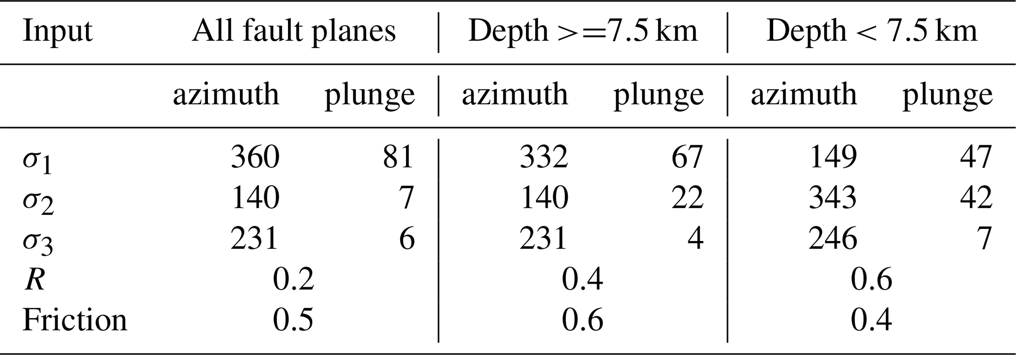
Our focal mechanisms are used to derive the directions of the principal stress axes σ1, σ2, σ3 with the python code StressInverse (Vavryčuk, 2014). The algorithm runs a stress inversion following Michael (1984) and modified to jointly invert for the fault orientations. To find the fault plane orientation, Vavryčuk (2014) includes the fault instability I, which can be evaluated from the friction on the fault plane, the shape ratio R and the inclination of the fault planes relative to the principal stress axes. The input into StressInverse is the strike, dip and rake of our 25 fault plane solutions (Table 2). To achieve an accuracy estimate we allow 100 runs with random noise and define the mean deviation of our fault planes of 30∘, which is reasonable considering a maximum Δrake of 68.2∘ (Table 2). The friction is allowed to vary between 0.4 and 1, and R varies between 0 and 1. The stress inversion is calculated for three different input data sets: all 25 fault planes (Fig. 8a), only focal mechanisms with a depth greater than 7.5 km (20 fault planes, Fig. 8b) and focal mechanisms with a depth shallower than 7.5 km (5 fault planes, Fig. 8c). The selected azimuth and plunge of σ1, σ2 and σ3 are given in Table 3. The separation into two data sets was necessary due to a wide variation of the confidence levels of σ1 and σ2 along the NW–SE direction (Fig. 8a). With a separation into shallow and deep events, this variation is reduced, indicating a depth dependency of the stress field (Fig. 8b). Nevertheless, due to the small amount of fault plane solutions in the depth range of 0.0–7.5 km, we find higher scatter of the confidence of the three principal stress axes (Fig. 8c). The measured and predicted fault planes from the stress inversion are shown in Fig. 8d). The predicted fault planes do not change for the different inversion runs.
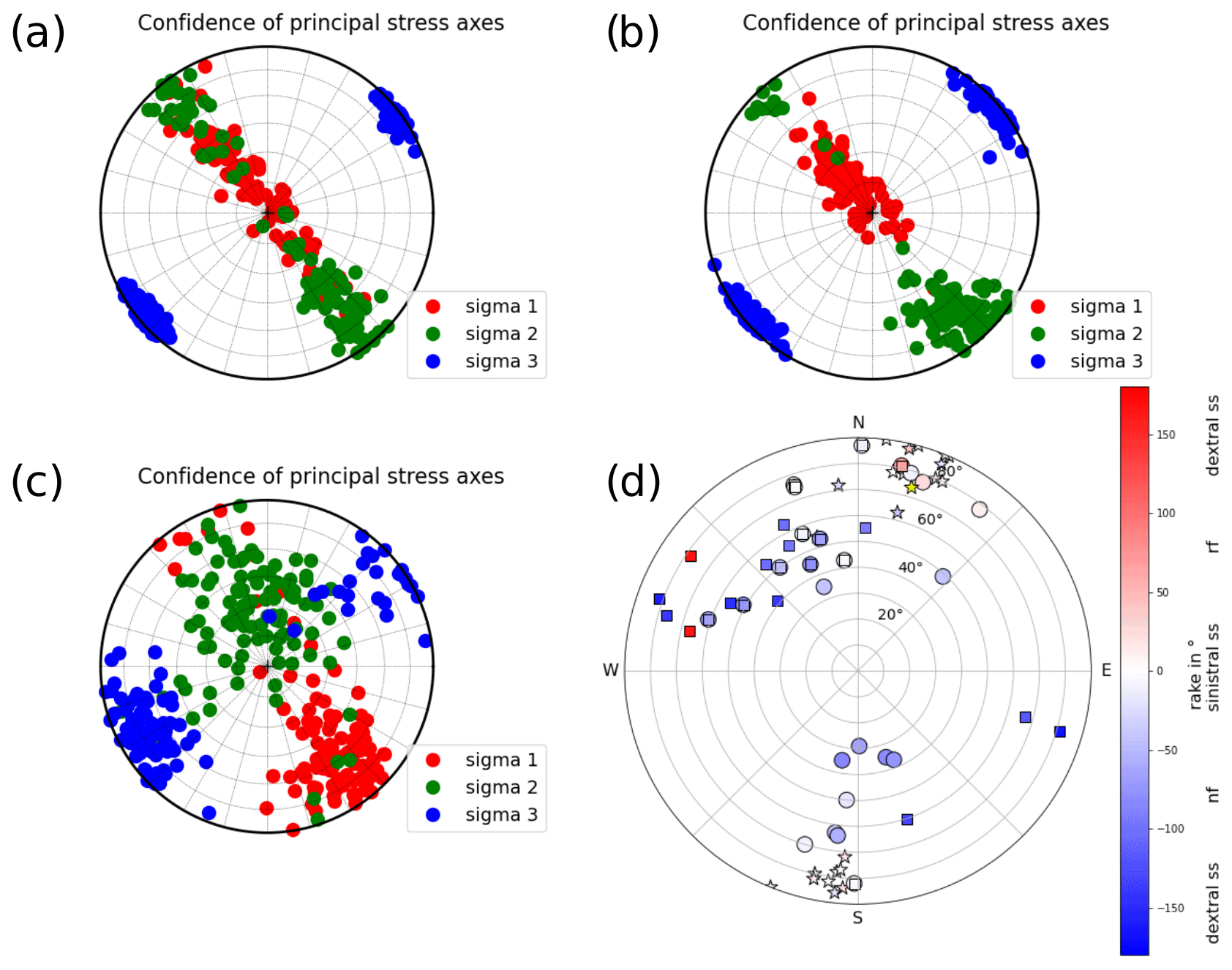
Figure 8(a) Confidence plot of the principal stress axes σ1, σ2 and σ3 after the stress inversion of all fault plane solutions (Table 2) for the 100 different noise realizations. (b) The same as Fig. 8a but only for fault plane solutions with a depth greater than 7.5 km. (c) The same as Fig. 8a but only for fault plane solutions with a depth less than 7.5 km. (d) Strike, dip and rake of all measured fault plane solutions (circles). The yellow star represents strike and dip of the 22 March 2003 earthquake (Stange and Brüstle, 2005). Other stars represent fault plane solutions calculated by Turnovsky (1981) for the earthquake series in 1978. Fault planes of StressInverse (Vavryčuk, 2014) are displayed by squares. Negative rake angles hint at normal faulting (nf) components, and positive angles hint at reverse faulting (rf) components. Events with a rake close to zero exhibit sinistral strike-slip (sinistral ss) components; events with rake angles close to −180 or 180∘ hint to dextral strike-slip (dextral ss).
Table 3Result of the stress inversion for all events, deep events and shallow events. Azimuth and plunge angles in ∘. R is the shape ratio.
5.1 Velocity model and station delay times
The finally selected minimum 1-D seismic velocity model ASZmod1 consists of 5 layers (Fig. 4a and b). The layer boundaries are based on the seismic refraction interpretation of Gajewski et al. (1987). Layers with very similar seismic velocities were combined during the inversion process to keep the model as simple as possible (Occam's principle). The determined seismic velocities increase with depth and they are well constrained between 2.50 and 18.25 km depth (Table 1). The layers between −2.00 to 2.50 km depth are not very stable due to the non-uniform distribution of rays and sources. Below 18.25 km depth we also have low resolution, as all events used for inversion occur above this point. The comparison with the LED models gives a good agreement with both the Swabian Jura and the Baden-Württemberg models (Fig. 4a). Our layer between 2.50 and 5.60 km depth is in good agreement with the Swabian Jura model, whereas the deeper layer has a higher agreement with the Baden-Württemberg model (Fig. 4a). The Swabian Jura model has a finer layering for the uppermost 2 km. We also used the Swabian Jura model as the input model for inversion, but due to the short horizontal ray length in comparison with the vertical ray length and the lack of events in the uppermost layers, the random seismic velocity starting models did not converge in the uppermost layers (Fig. 3); therefore, we chose the very simple layering.
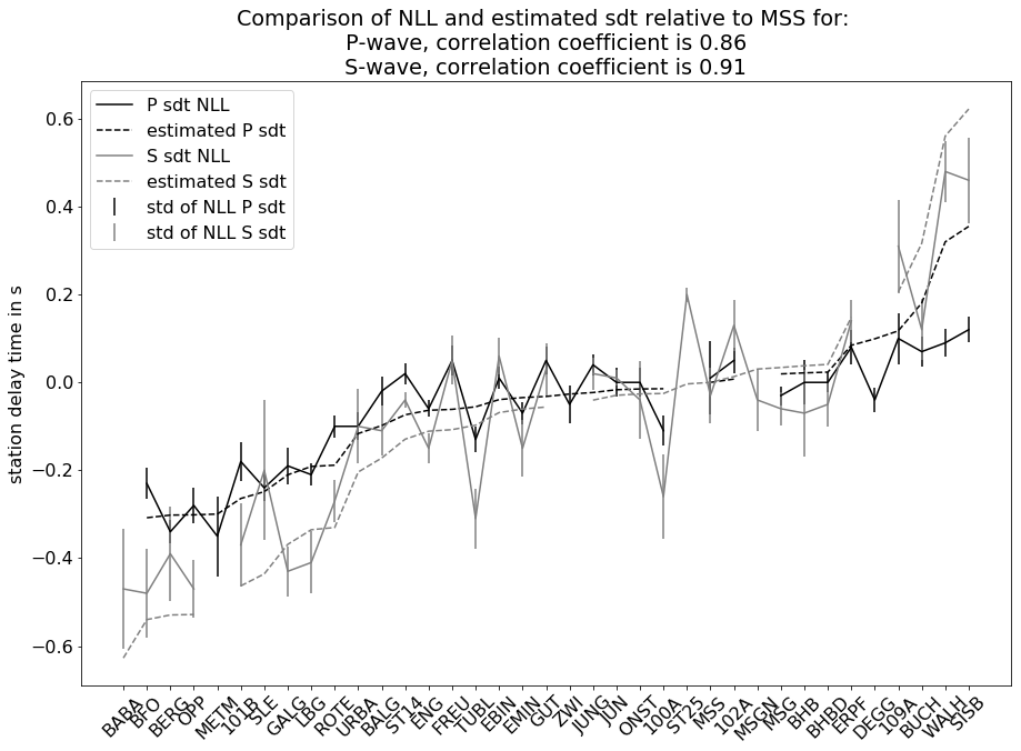
Figure 9Comparison of NLL station delay times (sdt) and estimated station delay times due to depth variations of the crystalline basement: P waves (black) and S waves (gray). Stations along the x axis are sorted from shallow to deep crystalline basement model depth.
The -ratio is between 1.67 and 1.75 for all layers and it decreases with depth. In comparison, the LED uses a constant ratio of 1.72 for Baden-Württemberg and 1.68 for the Swabian Alb, which agrees with our overall observed ratio (Fig. 4b, Bulletin-Files des Landeserdbebendienstes B-W, 2018). The higher ratio of 1.75 in the first layer is a result of the manually fixed seismic velocities during the inversion process. In the second layer the ratio is also 1.75, which may be caused by the numerical instability during the inversion of this layer and should be interpreted with care. In our best determined layers (layer 3 and 4) our model has similar ratios to the Swabian Jura model of the LED (Fig. 4b, Bulletin-Files des Landeserdbebendienstes B-W, 2018).
The station delay times of the P and S waves have a simple pattern of increasing delay times with distance to reference station MSS (Fig. 6). Their very low values in the area of the ASZ demonstrate that the vp and vs distributions of ASZmod1 represent the true seismic velocities in this area very well. Around the ASZ, the central Swabian Alb and the Molasse Basin are characterized by positive station delay times and thus slower seismic velocities along the propagation paths relative to ASZmod1. Other areas like the Black Forest exhibit negative delay times and thus faster seismic velocities than ASZmod1.
The lateral seismic velocity contrasts of the different near-surface layers of Baden-Württemberg are small in comparison to our station delay times. For this reason, we compare our station delay times with the lateral depth variations of the crystalline basement to find a possible relationship. The basement depth is described by the 3-D geological model of the Geological Survey of Baden-Württemberg (Rupf and Nitsch, 2008). Based on this model we estimate the vertical travel time at all our recording stations that have more than 5 of either P- or S-phase travel time picks using the seismic velocities of the first layer in ASZmod1 from the basement top to each recording station. For these values, we calculated the travel time differences of all stations relative to station MSS and compared the results (Fig. 9) with our real station delay times (Fig. 6). As result we find that the calculated travel time differences due to basement depth variations correlate to more than 85 % with our station delay times. Hence, basement depth variations are the main reason for the observed station delay times in our study region. The remaining 15 % of the station delay time terms may be explained by non-vertical ray path effects and lateral variations in seismic velocity due to different near-surface rock types. Furthermore, other lateral heterogeneities like dipping or wave-guiding layers may influence the station delay times as well.
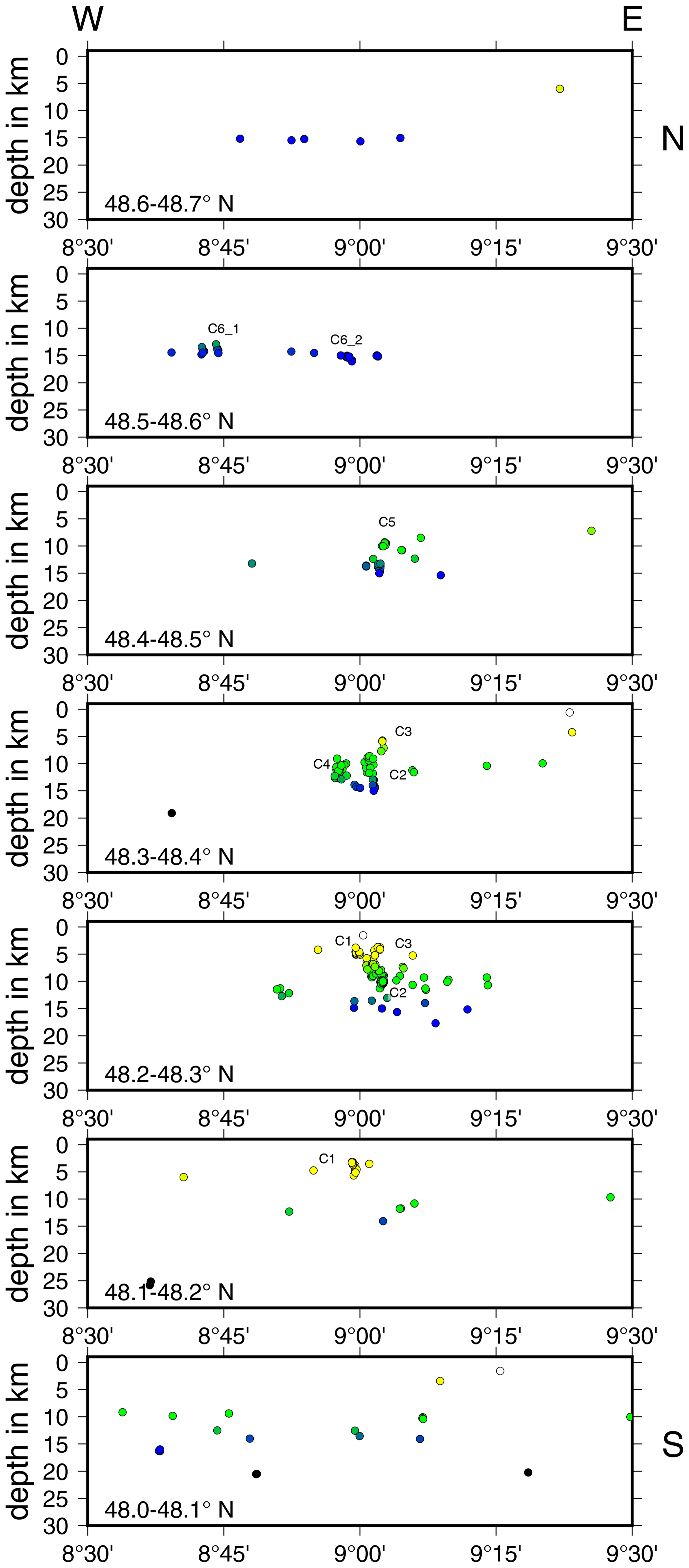
Figure 10Seismicity distribution of the ASZ from north (top) to south (bottom). Circles indicate hypocenters in the corresponding slice, color-coded by depth (as in Fig. 7); cluster codes are given for orientation.
5.2 Seismicity and fault plane solutions of the ASZ
The seismicity of the ASZ (Fig. 7) aligns almost N–S. Our relocated earthquakes occur in a depth range of 1 to 18 km. If we follow the seismicity distribution from south to north, the minimum hypocenter depth increases from around 3 to 5–14 km. Earthquakes below 18 km depth are rare at the ASZ. The top of the lower crust is at about 18–20 km depth (Gajewski and Prodehl, 1985; Aichroth et al., 1992); therefore, seismicity is concentrated in the upper crust. The hypocenters can be separated into several fault segments. This segmentation gets more obvious if we analyze E–W and N–S slices (Figs. 10, 11). To the north of the river Neckar (48.5–48.7∘ N), mainly deep (around 15 km depth) earthquakes occur, which can be separated into two clusters, one at 8.75∘ E (C6_1) and one at 8.95∘ E (C6_2, Fig. 10). Between the river Neckar and the town of Hechingen (48.3–48.5∘ N) we observe seismicity in the depth range of 5–15 km. There are three separate clusters, one west of 9∘ E, directly south of Hechingen (C4), and two clusters east of 9∘ E (C5 and C3). Near the town of Albstadt (48.2–48.3∘ N) the seismicity occurs across the whole seismically active depth range (1.5–18 km). Most of the seismicity happens between 9 and 9.1∘ E (C2, C3). At 2 to 8 km depth we find a small seismicity cluster southwest of Albstadt (8.9–9.0∘ E, C1). This cluster can be traced southward to 48.2∘ N (48.1–48.2∘ N, C1).
Most of the fault plane solutions are characterized by the typical NNE–SSW strike of the ASZ, but we also observe some events with NNW–SSE strike (Figs. 7, 8d, Table 2). Most of the events with a strike of NNE–SSW are characterized by steep fault planes (dip angle greater 60∘) and rake angles around 0∘, hinting at sinistral strike-slip. This is the typical or main faulting mechanism of the ASZ (Fig. 8d, Turnovski, 1981; Stange and Brüstle, 2005). We also observe one event with an NNE–SSW strike, a clear reverse faulting component and a steep fault plane of 86∘ (Fig. 8d). The other events with an NNE–SSW strike and the events with an NNW–SSE strike have lower dip angles (smaller 60∘) and mainly negative rake angles, hinting at normal faulting (Fig. 8d). The here-observed faulting behaviors can all be explained by a compressional stress regime with an average horizontal stress orientation of around 150∘ (Müller et al., 1992; Reinecker et al., 2010; Heidbach et al., 2016) acting on either the NNE–SSW- or NNW–SSE-oriented fault planes. The stress inversion following that of Vavryčuk (2014) also inverts for the probable rupturing fault plane in the current stress field (Fig. 8d). By comparing strike, dip and rake of the fault planes of the events in Table 2 with the probable fault plane of StressInverse, we observe that the NNW–SSE-oriented fault planes – typical for the ASZ – changed to their auxiliary fault planes, i.e., dextral strike-slip with a strike of WNW–ESE (Fig. 8d). As the aftershock distribution of the stronger events is NNE–SSW (e.g., Stange and Brüstle, 2005), as are our relocated events in Fig. 7, of course a sinistral fault plane with NNE–SSW strike is the preferred one. As explanation for this discrepancy we suggest that the ASZ is an inherited weak structure that needs much less stress for failure than the more probable WNW–ESE-oriented fault planes predicted by StressInverse. Ring et al. (2020) find that the ASZ coincides with the NNE–SSW-oriented boundary fault between the Triassic–Jurassic Spaichingen high and the Mid-Swabian basin, also hinting at a preexisting structure.
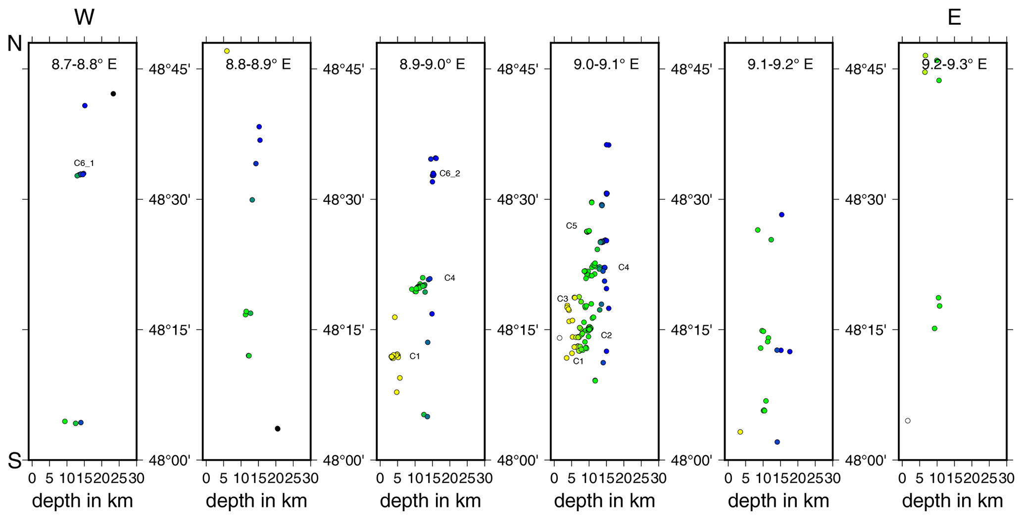
Figure 11Seismicity distribution of the ASZ from west (left) to east (right). Circles indicate hypocenters in the corresponding slice, color-coded by depth (as in Fig. 7); cluster codes are given for orientation.
The earthquake cluster C4 south of Hechingen (Figs. 10, 11) consists of events with normal faulting components (ev402, ev423, ev364) and the strike-slip event ev457 (Fig. 7). This cluster aligns along the boundary faults of the HZG and the events strike almost parallel to the HZG (Figs. 7, 8d). Other earthquakes close to the HZG boundary fault also strike almost parallel to the HZG (e.g., ev552, ev566, ev564). The depth extension of the HZG is not well known but is estimated from its extensional width and the dip angles of the main boundary faults at the surface. Based on these parameters, the boundary faults are thought to converge in about 2–3 km depth (Schädel, 1976). The faulting pattern of events close to HZG may indicate that the HZG boundary faults reach to greater depth, as already suggested by Schädel (1976) or Illies (1982). This may also imply that ev457 is a dextral strike-slip event, as is suggested by the result of the stress inversion. Relative event locations may help to identify the active fault planes in more detail using more data in future work.
5.3 Stress field around the ASZ
We inverted our fault plane solutions for the direction of the principal stress axes σ1, σ2, σ3 (Table 3). As for a combined run, the differentiation between σ1 and σ2 is difficult (Fig. 8a); we also inverted a split data set separated by the depth of 7.5 km (Fig. 8b, c). For depths shallower than 7.5 km, we observe the horizontal maximum stress with an azimuth of 149∘ to be greater than the vertical stress SV (Table 3). For a depth range greater than 7.5 km, we observe SV >. The depth dependence of the relative stress magnitudes is also known from other sites in the region. In the deep boreholes in Soultz (central Upper Rhine Graben), SV>SHmax is found in the upper ca. 2.5 km. Below this, SHmax>SV is valid to at least 5 km depth (Valley and Evans, 2003). Here has a direction of 169∘ E ± 14∘. In the southern Upper Rhine Graben, Plenefisch and Bonjer (1997) determined SHmax>SV in the upper crust to 15 km depth, whereas SV>SHmax was determined in the lower crust (> 15 km depth) from fault plane solutions. Our results indicate a shallower level (∼ 7 km) for the change of the maximum stress components, which may be due to a change in the rock rheology and needs to be studied with more data.
Our direction of is 140–149∘. The orientation of for southwestern Germany is estimated to be around 150∘ with a σ of 24∘ (Reinecker et al., 2010) and for all of western Europe it is 145∘ with a σ of 26∘ (Müller et al., 1992), which are both in agreement with our local orientation. Houlié et al. (2018) also observes a similar stress field in eastern Switzerland, southeast of our research area. Reinecker et al. (2010) suggest the gravitational potential energy of the Alpine topography as the main source of the local stress field because the stress field orientation in the northern Alpine foreland is always perpendicular to the Alpine front. Kastrup et al. (2004) also observe a change of stress field orientation with the Alpine front for the northern Alpine foreland in Switzerland. They explain the change of the orientation of the minimum horizontal stress Sh parallel to the Alpine front with a perturbation of the regional European stress field due to the indentation of the Adriatic Block. Müller et al. (1992) identify the plate-driving forces as sources of the maximum compression in the NW to NNW direction for all of western Europe, which are only perturbated by large geological structures like the Alps. As our study area is quite small, we cannot observe major lateral stress variations; however, the good coincidence with the regional stress field (Müller et al., 1992; Reinecker et al., 2010) is a strong indication that the driving tectonic forces of the seismicity of the ASZ are the regional plate-driving forces combined with the Alpine topography. Small-scale stress perturbations and variations of faulting mechanisms (Figs. 7 and 8) may be due to local heterogeneities of crustal material causing variations in rigidity or preexisting structures. These factors may also play a role in the segmentation of the ASZ, which will be analyzed in more details in the next few years.
We used our newly complemented seismicity catalog to invert for a robust new minimum 1-D seismic velocity model with station delay times for the ASZ region. These station delay times can be explained by the depth variation of the crystalline basement in the upper crust of Baden-Württemberg (Fig. 9). The relocated seismicity of the years 2011 to 2018 pictures the ASZ as a complex fault structure, with its current main active focus between the cities Albstadt and Tübingen on the Swabian Alb. The hypocenter error estimates clearly become smaller for events after 2016 due to the densified seismic station network of the LED and the complementing AASN stations. Thus, we expect another improvement and an increase in detectable events from 2019 onwards due to our additionally installed StressTransfer stations (Fig. 1). Future work will take advantage of the densified seismic station network and focus on small-magnitude event detection based on template matching in the area of the ASZ.
Most of the seismicity takes place in a N–S-oriented band east of 9∘ E (Fig. 7). A spatial clustering of events is found,m which may indicate separate fault planes. If such a separation can be verified in the future, this segmentation would limit the maximum size of earthquake rupture planes and its related hazard potential (Grünthal and the GSHAP Region 3 Working Group, 1999). Nevertheless, we find the shallow cluster C1 slightly separated to the west from the other events, as well as the deeper cluster C4 near Hechingen. Furthermore, we observe clear normal faulting events, which were so far not observed for the ASZ. A relation of the clusters C4 with a continuation of the HZG into the crystalline basement is possible and needs further observational constraints to better describe the seismic potential of the HZG. Ongoing work will determine relative locations for all events from 2016 and following years to obtain an even sharper image of the fault planes of the ASZ. We will also continue complementing our catalog with new earthquakes and fault plane solutions after 2018.
The estimated has a NNW–SSW trend. This is in good agreement with other studies (Müller et al., 1992; Kastrup et al., 2004; Reinecker et al., 2010; Houlié et al., 2018). As plausible driving forces of our local stress field, we identify the regional plate driving forces and the Alpine topography (Müller et al., 1992; Kastrup et al., 2004; Reinecker et al., 2010). In the upper part of the crust exceeds SV (Fig. 8). Below about 7–8 km depth SV seems to be the dominating stress component. Within the StressTransfer project, similar investigations are planned for the URG to the west and the Molasse Basin southeast of the ASZ to get a better understanding of the stress field in the northern Alpine foreland of southwestern Germany.
Table A1Definition of the error quality relationship; lp-ep represents the time window in which the final pick is manually selected.

Table A2Classification of the qualities used for focal mechanisms. Δx represents Δstrike, Δdip and Δrake. The lowest quality of all three parameters is given to the fault plane solution.

The preprocessing and picking analyses of the data were done in Python with the open-source toolbox ObsPy (Beyreuther et al., 2010, https://github.com/obspy/obspy/wiki, last access: 30 September 2020). For further data analyses we used the freely available programs VELEST (Version 4.5, Kissling et al., 1994, 1995; Singer et al., 2017, https://seg.ethz.ch/software/velest. html, last access: 30 September 2020), NonLinLoc (Lomax et al., 2000, 2017, http://alomax.free.fr/nlloc/index.html, last access: 30 September 2020), FocMec (Snoke, 2003, 2017, http://ds.iris.edu/pub/programs/focmec/, last access: 30 September 2020) and StressInverse (Vavryčuk, 2014, 2020, https://www.ig.cas.cz/en/stress-inverse/, last access: 24 February 2021). All figures were created with either the Matplotlib library in Python (Hunter, 2007, https://matplotlib.org/, last access: 30 September 2020) or the Generic Mapping Tools (GMT, Wessel et al., 2019, https://www.generic-mapping-tools.org/, last access: 30 September 2020).
We used the restricted bulletin files of the state earthquake service of Baden-Württemberg (LED), which were provided to us by the LED (Bulletin-Files des Landeserdbebendienstes B-W, 2018, https://lgrb-bw.de/erdbeben/index_html?lang=1, last access: 30 September 2020). We analyzed the data of four AlpArray stations of the Z3 network, which will become available on 1 April 2022 to people outside the AlpArray Working Group (http://www.alparray.ethz.ch/en/seismic_network/backbone/data-access/, last access: 30 September 2020). The data of the StressTransfer Network are currently restricted and will become available on 1 April 2022 (Mader and Ritter, 2021).
The supplement related to this article is available online at: https://doi.org/10.5194/se-12-1389-2021-supplement.
The complete member list of the AlpArray Working Group can be found at http://www.alparray.ethz.ch.
SM carried out the fieldwork, analyzed the data with self-written and open-source programs, and prepared the manuscript and figures. JRRR and KR formulated the project, obtained funding and started the fieldwork. All three were involved in writing the manuscript. The AlpArray Working Group organized and coordinated the AlpArray Seismic Network operation.
The authors declare that they have no conflict of interest.
This article is part of the special issue “New insights into the tectonic evolution of the Alps and the adjacent orogens”. It is not associated with a conference.
We thank the State Earthquake Service of Baden-Württemberg (Landeserdbebendienst B-W) for providing waveform data, pick files and internal information (Az4784//18_3303). We thank Andrea Brüstle, Tobias Diehl and Dietrich Lange for programming- and program-related support and helpful discussions. Waveform recordings were provided by the AlpArray Seismic Network (2015). Recording instruments were provided by the KArlsruhe BroadBand Array, Karlsruhe Institute of Technology. Sarah Mader and Joachim R. R. Ritter were supported by the Deutsche Forschungsgemeinschaft (DFG) through grant RI1133/13-1, and Klaus Reicherter was supported through grant RE1361/31-1 within the framework of DFG Priority Programme “Mountain Building Processes in Four Dimensions (MB-4D)” (SPP 2017). Felix Bögelspacher, Felix Pappert, Leon Merkel, Sergio León-Ríos and Werner Scherer assisted the fieldwork. Michael Frietsch helped with the data management. We thank numerous people and associations for supporting the installation of the mobile recording instruments on their land. We acknowledge support by the KIT-Publication Fund of the Karlsruhe Institute of Technology.
We thank the AlpArray Seismic Network Team: György Hetényi, Rafael Abreu, Ivo Allegretti, Maria-Theresia Apoloner, Coralie Aubert, Simon Besançon, Maxime Bès de Berc, Götz Bokelmann, Didier Brunel, Marco Capello, Martina Čarman, Adriano Cavaliere, Jérôme Chèze, Claudio Chiarabba, John Clinton, Glenn Cougoulat, Wayne C. Crawford, Luigia Cristiano, Tibor Czifra, Ezio D'alema, Stefania Danesi, Romuald Daniel, Anke Dannowski, Iva Dasović, Anne Deschamps, Jean-Xavier Dessa, Cécile Doubre, Sven Egdorf, ETHZ-SED Electronics Lab, Tomislav Fiket, Kasper Fischer, Wolfgang Friederich, Florian Fuchs, Sigward Funke, Domenico Giardini, Aladino Govoni, Zoltán Gráczer, Gidera Gröschl, Stefan Heimers, Ben Heit, Davorka Herak, Marijan Herak, Johann Huber, Dejan Jarić, Petr Jedlička, Yan Jia, Hélène Jund, Edi Kissling, Stefan Klingen, Bernhard Klotz, Petr Kolínský, Heidrun Kopp, Michael Korn, Josef Kotek, Lothar Kühne, Krešo Kuk, Dietrich Lange, Jürgen Loos, Sara Lovati, Deny Malengros, Lucia Margheriti, Christophe Maron, Xavier Martin, Marco Massa, Francesco Mazzarini, Thomas Meier, Laurent Métral, Irene Molinari, Milena Moretti, Anna Nardi, Jurij Pahor, Anne Paul, Catherine Péquegnat, Daniel Petersen, Damiano Pesaresi, Davide Piccinini, Claudia Piromallo, Thomas Plenefisch, Jaroslava Plomerová, Silvia Pondrelli, Snježan Prevolnik, Roman Racine, Marc Régnier, Miriam Reiss, Joachim Ritter, Georg Rümpker, Simone Salimbeni, Marco Santulin, Werner Scherer, Sven Schippkus, Detlef Schulte-Kortnack, Vesna Šipka, Stefano Solarino, Daniele Spallarossa, Kathrin Spieker, Josip Stipčević, Angelo Strollo, Bálint Süle, Gyöngyvér Szanyi, Eszter Szücs, Christine Thomas, Martin Thorwart, Frederik Tilmann, Stefan Ueding, Massimiliano Vallocchia, Luděk Vecsey, René Voigt, Joachim Wassermann, Zoltán Wéber, Christian Weidle, Viktor Wesztergom, Gauthier Weyland, Stefan Wiemer, Felix Wolf, David Wolyniec, Thomas Zieke, Mladen Živčić and Helena Žlebčíková.
The article processing charges for this open-access publication were covered by the Karlsruhe Institute of Technology (KIT).
This paper was edited by Christian Sue and reviewed by Thomas Plenefisch and one anonymous referee.
Aichroth, B., Prodehl, C., and Thybo, H.: Crustal structure along the Central Segment of the EGT from seismic-refraction studies, Tectonophysics, 207, 43–64, 1992.
Aki, K. and Richards, P. G.: Quantitative Seismology: Theory and Methods, edited by: Freeman, W. H., San Francisco, CA, Second Edition, 1, 558 pp., 2002.
Akinci, A., Mejia, J., and Jemberie, A. L.: Attenuative dispersion of P waves and crustal Q in Turkey and Germany, Pure Appl. Geophys., 161, 73–91, 2004.
AlpArray Seismic Network: AlpArray Seismic Network (AASN) temporary component, AlpArray Working Group, Other/Seismic Network, https://doi.org/10.12686/alparray/z3_2015, 2015.
Amante, C. and Eakins, B. W.: ETOPO1 1 Arc-Minute Global Relief Model: Pocedures, Data Sources and Analysis, NOAA Technical Memorandum NESDIS NGDC-24, National Geophysical Data Center, NOAA, 19 pp, 2009.
Asch, K.: IGME Million International Geological Map of Europe and Adjacent Areas – final version for the internet - BGR, Hannover, 1 map [data set], https://www.bgr.bund.de/EN/Themen/Sammlungen-Grundlagen/GG_geol_Info/Karten/Europa/IGME5000/IGME_Project/IGME_Downloads.html?nn=1556388, 2005.
Becker, A.: An attempt to define a “neotectonic period” for Central and northern Europe, Geol. Rundsch., 82, 67–83, 1993.
Beyreuther, M., Barsch, R., Krischer, L., Megies, T., Behr, Y., and Wassermann, J.: ObsPy: A Python Toolbox for Seismology [data set], available at: https://github.com/obspy/obspy/wiki (last access: 30 September 2020), 2010.
Bonjer, K.-P.: Seismicity pattern and style of seismic faulting at the eastern borderfault of the southern Rhine Graben, Tectonophysics, 275, 41–69, 1997.
Bulletin-Files des Landeserdbebendienstes B-W: Ref. 98 im Landesamt für Geologie, Rohstoffe und Bergbau im Regierungspräsidium Freiburg (https://lgrb-bw.de/erdbeben/index_html?lang=1) [data set], Az4784//18_3303, 2018.
Diehl, T., Kissling, E., and Bormann, P.: Tutorial for consistent phase picking at local to regional distances, in: New Manual of Seismological Observatory Practice 2 (NMOSOP-2), edited by: Bormann, P., Potsdam: Deutsches Geoforschungszentrum GFZ, p. 1.21, 2012.
Gajewski, D. and Prodehl, C.: Crustal structure beneath the Swabian Jura, SW Germany, from seismic refraction investigations, J. Geophys., 56, 69–80, 1985.
Gajewski, D., Holbrook, W. S., and Prodehl, C.: A three-dimensional crustal model of southwest Germany derived from seismic refraction data, Tectonophysics, 142, 49–70, 1987.
Geyer, O. F. and Gwinner, M. P.: Geologie von Baden-Württemberg, 5 Edn., edited by: Geyer, M., Nitsch, E., and Simon, T., Schweitzerbart, Stuttgart, Germany, 627 pp, 2011.
Gräber,, F.: Lokalbebentomographie mit P-Wellen in Long Valley, Kalifornien, und die Möglichkeiten einer Anwendung im südlichen Rheingraben, Diplomarbeit (diploma thesis), Geophysical Institute, TU Karlsruhe, Germany and Institute of Geophysics, ETH Zürich, Switzerland, 144 pp, 1993.
Grünthal, G. and the GSHAP Region 3 Working Group: Seismic hazard assessment for Central, North and Northwest Europe: GSHAP Region 3. Anali di Geofisica, 42, 999–1011, 1999.
Haessler, H., Hoang-Trong, P., Schick, R., Schneider, G., and Strobach, K.: The September 3, 1978, Swabian Jura Earthquake, Tectonophysics, 68, 1–14, 1980.
Heidbach, O., Rajabi, M., Reiter, K., and Ziegler, M., WSM Team: World Stress Map Database Release 2016, V. 1.1, GFZ Data Services, https://doi.org/10.5880/WSM.2016.001, 2016.
Hetényi, G., Molinari, I., Clinton, J., Bokelmann, G., Bondár, I., Crawford, W. C., Dessa, J.-X., Doubre, C., Friederich, W., Fuchs, F., Giardini, D., Gráczer, Z., Handy, M. R., Herak, M., Jia, Y., Kissling, E., Kopp, H., Korn, M., Margheriti, L., Meier, T., Mucciarelli, M., Paul, A., Pesaresi, D., Piromallo, C., Plenefisch, T., Plomerová, J., Ritter, J., Rümpker, G., Šipka, V., Spallarossa, D., Thomas, C., Tilmann, F., Wassermann, J., Weber, M., Wéber, Z., Wesztergom, V., Živčić, M., AlpArray Seismic Network Team, AlpArray OBS Cruise Crew, and AlpArray Working Group: The AlpArray Seismic Network: a large-scale European experiment to image the Alpine orogen, Surv. Geophys., 1–25, https://doi.org/10.1007/s10712-018-9472-4, 2018.
Hiller, W.: Eine Erdbebenwarte im Gebiet der Schwäbischen Alb, Z. Geophysik, 9, 230–234, 1933.
Houlié, N., Woessner, J., Giardini, D., and Rothacher, M.: Lithosphere strain rate and stress field orientations near the Alpine arc in Switzerland, Sci. Rep., 8, 1–14, 2018.
Hunter, J. D.: “Matplotlib: A 2D Graphics Environment”, Comput. Sci. Eng., 9, 90–95, 2007.
Husen, S., Kissling, E., Deichmann, N., Wiemer, S., Giardini, D., and Baer, M.: Probabilistic earthquake location in complex three-dimensional velocity models: Application to Switzerland, J. Geophys. Res., 108, 2077, https://doi.org/10.1029/2002JB001778, 2003.
Illies, J. H.: Der Hohenzollerngraben und Intraplattenseismizität infolge Vergitterung lamellärer Scherung mit einer Riftstruktur, Oberrhein. Geol. Abh., 31, 47–78, 1982.
Kastrup, U., Zoback, M. L., Deichmann, N., Evans, K. F., Giardini, D., and Michael, A. J.: Stress field variations in the Swiss Alps and the northern Alpine foreland derived from inversion of fault plane solutions, J. Geophys. Res., 109, B01402, https://doi.org/10.1029/2003JB002550, 2004.
Kennett, B. L. N., Engdahl, E. R., and Buland, R.: Constraints on seismic velocities in the Earth from traveltimes, Geophys. J. Int., 122, 108–124, 1995.
Kissling, E., Ellsworth, W. L., Eberhart-Phillips, D., and Kradolfer, U.: Initial reference models in local earthquake tomography, J. Geophys. Res.-Sol. Ea., 99, 19635–19646, 1994.
Kissling, E., Kradolfer, U., and Maurer, H.: Program VELEST user’s guide – Short Introduction, Int. Report, Institute of Geophysics, ETH, Zürich, available at: https://seg.ethz.ch/software/velest.html, 26 pp, 1995.
Kunze, T.: Seismotektonische Bewegungen im Alpenbereich, PhD thesis, University Stuttgart, Germany, 167 pp, 1982.
Leydecker, G.: Erdbebenkatalog für Deutschland mit Randgebieten für die Jahre 800 bis 2008, Geologisches Jahrbuch, E 59, E. Schweizerbart'sche Verlagsbuchhandlung, Stuttgart, 198 pp., 2011.
Lomax, A., Virieux, J., Volant, P., and Berge-Thierry, C.: Probabilistic earthquake location in 3D and layered models: introduction to a Metropolis-Gibbs method and comparison with linear locations, edited by: Thurber, C. and Rabinowitz, N., Advances in seismic event location, Springer, Dordrecht, 18, 101–134, 2000.
Lomax, A.: NonLinLoc software – Probabilistic, Non-Linear, Global-Search Earthquake Location in 3D Media available at: http://alomax.free.fr/nlloc/index.html, last access: 30 September 2020, 2017.
Mader, S. and Ritter, J. R. R.: The StressTransfer Seismic Network – An Experiment to Monitor Seismically Active Fault Zones in the Northern Alpine Foreland of Southwestern Germany, Seismol. Res. Lett., 92, 1773–1787, https://doi.org/10.1785/0220200357, 2021.
Meschede, M. and Warr, L. N.: The Geology of Germany: A Process-Oriented Approach, Regional Geology Reviews, edited by: Oberhänsli, R., de Wit, M. J., and Roure, F. M., Springer Nature Switzerland AG, 304 pp, 2019.
Michael, A. J.: Determination of stress from slip data: Faults and folds, J. Geophys. Res., 89, 11517–11526, 1984.
Müller, B., Zoback, M. L., Fuchs, K., Mastin, L., Gregersen, S., Pavoni, N., Stephansson, O., and Ljunggren, C.: Regional patterns of tectonic stress in Europe, J. Geophys. Res., 97, 11783–11803, 1992.
NOAA National Geophysical Data Center: ETOPO1 1 Arc-Minute Global Relief Model [data set], NOAA National Centers for Environmental Information, https://doi.org/10.7289/V5C8276M, 2009.
Oncescu, M. C., Rizescu, M., and Bonjer, K. P.: SAPS – a completely automated and networked seismological acquisition and processing system, Comp. Geosci., 22, 89–97, 1996.
Plenefisch, T. and Bonjer, K.-P.: The stress field in the Rhine Graben area inferred from earthquake focal mechanisms and estimation of frictional parameters, Tectonophysics, 275, 71–97, 1997.
Podvin, P. and Lecomte, I.: Finite difference computation of traveltimes in very contrasted velocity models: a massively parallel approach and its associated tools, Geophys. J. Int., 105, 271–284, 1991.
Regierungspräsidium Freiburg: Landesamt für Geologie, Rohstoffe und Bergbau (Hrsg.): LGRB-Kartenviewer – Layer GÜK300: Tektonik, available at: https://maps.lgrb-bw.de/, last access: 28 March 2019.
Regierungspräsidium Freiburg: Landesamt für Geologie, Rohstoffe und Bergbau: Last felt earthquakes in Baden-Württemberg, available at: https://lgrb-bw.de/erdbeben/erdbebenmeldung, last access: 28 August 2020.
Reicherter, K., Froitzheim, N., Jarosinski, M., Badura, J., Franzke, H. J., Hansen, M., and Stackebrandt, W.: Alpine tectonics north of the Alps, The geology of central Europe, 2, 1233–1285, 2008.
Reinecker, J. and Schneider, G.: Zur Neotektonik der Zollernalb: Der Hohenzollerngraben und die Albstadt-Erdbeben, Jahresberichte und Mitteilungen des Oberrheinischen Geologischen Vereins, 391–417, 2002.
Reinecker, J., Tingay, M., Müller, B., and Heidbach, O.: Present-day stress orientation in the Molasse Basin, Tectonophysics, 482, 129–138, 2010.
Ring, U. and Bolhar, R.: Tilting, uplift, volcanism and disintegration of the South German block, Tectonophysics, 795, 228611, https://doi.org/10.1016/j.tecto.2020.228611, 2020.
Rupf, I. and Nitsch, E.: Das Geologische Landesmodell von Baden-Württemberg: Datengrundlagen, technische Umsetzung und erste geologische Ergebnisse, Regierungspräsidium Freiburg – Abteilung 9, Landesamt für Geologie, Rohstoffe und Bergbau, 82 pp., 2008.
Schädel, K.: Geologische Übersichtskarte 1:100.000 C7918 Albstadt und Erläuterungen. Geologisches Landesamt Baden-Württemberg, Freiburg i. Br., 44 pp, 1976.
Schneider, G.: Seismizität und Seismotektonik der Schwäbischen Alb, F. Enke Verlag, Stuttgart, Germany, 79 pp., 1971.
Schneider, G.: Die Erdbeben in Baden-Württemberg: 1963–1972, Inst. für Geophysik der Univ. Stuttgart, Germany, 47 pp., 1973.
Schneider, G.: The earthquake in the Swabian Jura of 16 Nov. 1911 and present concepts of seismotectonics, Tectonophysics, 53, 279–288, 1979.
Schneider, G.: Das Beben vom 3. September 1978 auf der Schwäbischen Alb als Ausdruck der seismotektonischen Beweglichkeit Suedwestdeutschlands, Jahresberichte und Mitteilungen des Oberrheinischen Geologischen Vereins, N. F., 62, 143–166, 1980.
Schneider, G.: Beziehungen zwischen Erdbeben und Strukturen der Süddeutschen Großscholle, Neues Jahrbuch für Geologie und Palaäntologie – Abhandlungen, 189, 275–288, 1993.
Sieberg, A. and Lais, R.: Das mitteleuropäische Erdbeben vom 16.11.1911, Bearbeitung der makroseismischen Beobachtungen, Veröffentlichungen der Reichsanstalt für Erdbebenforschung Jena, H. 4, Jena, Germany, 106 pp., 1925.
Singer, J., Kissling, E., and Diehl, T.: VELEST, Version 4.5 provided by Kissling, E., Version 3.1, available at: https://seg.ethz.ch/software/velest.html, last access: 30 September 2020, 2017.
Snoke, J. A.: FOCMEC: Focal mechanism determinations. International Handbook of Earthquake and Engineering Seismology, 85, 1629–1630, 2003.
Snoke, A.: FOCMEC, available at: http://ds.iris.edu/pub/programs/focmec/, last access 30 September 2020, 2017.
Stange, S.: Erdbebenüberwachung Baden-Württemberg – Das modernisierte Starkbeben- und Detektionsmessnetz. LGRB – Nachricht, Regierungspräsidium Freiburg, Nr. 2018/07, 2 pp., 2018.
Stange, S. and Brüstle, W.: The Albstadt/Swabian Jura seismic source zone reviewed through the study of the earthquake of March 22, 2003, Jahresberichte und Mitteilungen des Oberrheinischen Geologischen Vereins, 391–414, 2005.
Tarantola, A. and Valette, B.: Inverse problems = quest for information, J. Geophys., 50, 159–170, 1982.
Tozer, B., Sandwell, D. T., Smith, W. H., Olson, C., Beale, J. R., and Wessel, P.: Global bathymetry and topography at 15 arc sec: SRTM15+, Earth Space Sci., 6, 1847–1864, 2019.
Turnovsky, J.: Herdmechanismen und Herdparameter der Erdbebenserie 1978 auf der Schwäbischen Alb, PhD thesis, University Stuttgart, Germany, 109 pp., 1981.
Tyagunov, S., Grünthal, G., Wahlström, R., Stempniewski, L., and Zschau, J.: Seismic risk mapping for Germany, Nat. Hazards Earth Syst. Sci., 6, 573–586, https://doi.org/10.5194/nhess-6-573-2006, 2006.
Valley, B. and Evans, K. F.: Stress state at Soultz to 5 km depth from wellbore failure and hydraulic observations, Proceedings, Thirty-Second Workshop on Geothermal Reservoir Engineering, Stanford University, Stanford, California, 10 pp., 2007.
Vavryčuk, V.: Iterative joint inversion for stress and fault orientations from focal mechanisms, Geophys. J. Int., 199, 69–77, https://doi.org/10.1093/gji/ggu224, 2014.
Vavryčuk, V.: STRESSINVERSE, available at: https://www.ig.cas.cz/en/stress-inverse/, last access 24 February 2021, 2020.
Wessel, P., Luis, J. F., Uieda, L., Scharroo, R., Wobbe, F., Smith, W. H. F., and Tian, D: The Generic Mapping Tools version 6., Geochem. Geophys. Geosys., 20, 5556–5564, https://doi.org/10.1029/2019GC008515, 2019.
Wetzel, H.-U. and Franzke, H. J.: Lassen sich über die Fernerkundung erweiterte Kenntnisse zur seismogenen Zone Bodensee-Stuttgart (9∘-Ost) gewinnen?, Publikationen der Deutschen Gesellschaft für Photogrammetrie und Fernerkundung, 12, 339–347, 2003.
- Abstract
- Introduction
- Geological and tectonic setting
- Earthquake data and station network
- Data processing
- Results and discussion
- Conclusion and outlook
- Appendix A
- Code availability
- Data availability
- Team list
- Author contributions
- Competing interests
- Special issue statement
- Acknowledgements
- Financial support
- Review statement
- References
- Supplement