the Creative Commons Attribution 4.0 License.
the Creative Commons Attribution 4.0 License.
 | 06 Jul 2021
Magma ascent mechanisms in the transition regime from solitary porosity waves to diapirism
Janik Dohmen
Harro Schmeling
In partially molten regions inside the Earth, melt buoyancy may trigger upwelling of both solid and fluid phases, i.e., diapirism. If the melt is allowed to move separately with respect to the matrix, melt perturbations may evolve into solitary porosity waves. While diapirs may form on a wide range of scales, porosity waves are restricted to sizes of a few times the compaction length. Thus, the size of a partially molten perturbation in terms of compaction length controls whether material is dominantly transported by porosity waves or by diapirism. We study the transition from diapiric rise to solitary porosity waves by solving the two-phase flow equations of conservation of mass and momentum in 2D with porosity-dependent matrix viscosity. We systematically vary the initial size of a porosity perturbation from 1.8 to 120 times the compaction length.
If the perturbation is of the order of a few compaction lengths, a single solitary wave will emerge, either with a positive or negative vertical matrix flux. If melt is not allowed to move separately to the matrix a diapir will emerge. In between these end members we observe a regime where the partially molten perturbation will split up into numerous solitary waves, whose phase velocity is so low compared to the Stokes velocity that the whole swarm of waves will ascend jointly as a diapir, just slowly elongating due to a higher amplitude main solitary wave.
Only if the melt is not allowed to move separately to the matrix will no solitary waves build up, but as soon as two-phase flow is enabled solitary waves will eventually emerge. The required time to build them up increases nonlinearly with the perturbation radius in terms of compaction length and might be too long to allow for them in nature in many cases.
- Article
(2478 KB) - Full-text XML
- BibTeX
- EndNote


In geodynamic settings such as mid-ocean ridges, hotspots, subduction zones, or orogenic belts partial melts are generated within the asthenosphere or lower continental crust and ascend by fluid migration within deforming rocks (e.g., Sparks and Parmentier, 1991; Katz, 2008; Keller et al., 2017; Schmeling et al., 2019). Inherent tectonic or rock heterogeneities in such systems may result in spatially varying melt fractions on length scales varying over several orders of magnitudes. These length scales play an important role in determining whether melt anomalies may rise as porous waves (Jordan et al., 2018) or by other mechanisms such as diapirs (Rabinowicz et al., 1987), focused channel networks (Spiegelman et al., 2001), or dikes (Rivalta et al., 2015). Here we focus on the effect of the length scale on the formation and evolution of buoyancy-driven porous waves or diapirs.
The physics of fluid moving relatively to a viscously deformable porous matrix were first described by McKenzie (1984), and it was later shown by several authors that these equations allow for the emergence of solitary porosity waves (Scott and Stevenson, 1984; Barcilon and Lovera 1989; Wiggins and Spiegelman, 1995). Porosity waves are regions of localized excess fluid that ascend with permanent shape and constant velocity, controlled by compaction and decompaction of the surrounding matrix. They have been extensively studied as mechanisms transporting geochemical signatures or magma through the asthenosphere, lower crust, and middle crust (e.g., Watson and Spiegelman, 1994; McKenzie, 1984; Connolly, 1997; Connolly and Podladchikov, 2013, Jordan et al., 2018, Richard et al., 2012). It has been shown that the dynamics of porous waves strongly depend on the porosity dependence of the matrix rheology (e.g., Connolly and Podladchikov, 1998, 2015; Yarushina et al., 2015; Omlin et al., 2017; Dohmen et al., 2019). However, one open question is how the length scale of solitary porosity waves relates to an arbitrary length scale of a possible porosity anomaly in given geodynamic settings.
The size of a solitary porosity wave is usually of the order of a few compaction lengths (McKenzie, 1984; Scott and Stevenson, 1984; Simpson and Spiegelman, 2011), but this length scale varies over a few orders of magnitude, depending on the shear and volume viscosity of the matrix, fluid viscosity, and permeability (see Eq. 19) with typical values of 100–10 000 m (McKenzie, 1984; Spiegelman, 1993a, b). However, partially molten regions in the lower crust or upper mantle are prone to gravitational instabilities such as Rayleigh–Taylor instabilities or diapirism (e.g., Griffith, 1986; Bittner and Schmeling, 1995; Schmeling et al., 2019). Originating from the Greek “diapeirein”, i.e., “to pierce through”, diapirism describes the “buoyant upwelling of relatively light rock” (Turcotte and Schubert, 1982) through and into a denser overburden. In the general definition, the rheology of the diapir and ambient material is not specified and both can be ductile, as in our case. Buoyancy may be of compositional or phase-related origin, e.g., due to the presence of non-segregating partial melt (Wilson, 1989). In this model we describe a diapir as a partially molten perturbation, whose rising velocity, characterizable by the Stokes velocity, is lower than the corresponding solitary-wave phase velocity.
As characteristic wavelengths of Rayleigh–Taylor instabilities may be similar but also of significantly different order to those of porosity waves, and the Stokes velocity is strongly affected by the spatial expansion, the question arises as to how these two mechanisms interact and what the transition from a porosity wave to a rising partially molten diapir looks like. Scott (1988) already investigated a similar scenario. He calculated porosity waves changing the compaction length by altering the constant shear to volume viscosity ratio. In contrast, we vary the radius of a partially molten perturbation in terms of compaction lengths while keeping the porosity-dependent viscosity law the same. While Scott (1988) was not able to reach the single-phase flow endmember due to his setup, we can reach this endmember with our description and can explore the transition.
In this work we will address the question of length scale of a partially molten region with respect to the length scale of a solitary porosity wave by varying the sizes of initial porosity perturbations. We further focus on the numerical implications on modeling magma transport.
2.1 Governing equations
The formulation of the governing equations for the melt-in-solid two-phase flow dynamics is based on McKenzie (1984), Spiegelman and McKenzie (1987), and Schmeling (2000), assuming an infinite Prandtl number, a low fluid viscosity with respect to the effective matrix viscosity, zero surface tension, and the Boussinesq approximation. In the present formulation, the Boussinesq approximation assumes the same constant density for the solid and fluid except for the buoyancy terms of the momentum equations for the solid and fluid. In the following all variables associated with the pore fluid (melt) have the subscript f and those associated with the solid matrix have the subscript s. The equation for the conservation of the mass of the melt is
and the mass conservation of the solid is
φ is the volumetric rock porosity (often called melt fraction), vf and vs are the fluid and solid velocities, respectively. The momentum equations are given as a generalized Darcy equation for the fluid separation flow
where ρf is the fluid density and Pf is the fluid pressure (including the lithostatic pressure), whose gradient is driving the fluid segregation by porous flow, μ is the melt dynamic viscosity, and g is the gravitational acceleration. kφ is the permeability that depends on the rock porosity
with n being the power law exponent constant, usually equal to 2 or 3. This relation is known as the Kozeny–Carman relation (e.g., Costa, 2006). The Stokes equation for the mixture is given as
where is the density of the melt–solid mixture and τ is the effective viscous stress tensor of the matrix, including both shear and compaction components
where ζ is the volume viscosity, and vsi and vsj are the ith and jth component of vs. The linearized equation of state for the mixture density is given as
with ρ0 as the solid density and . The shear and volume viscosity are given by the equations
and
where η0 is the constant intrinsic shear viscosity of the matrix.
As in both Eqs. (3) and (5), Pf is the fluid pressure (see McKenzie, 1984, Appendix A), these equations can be merged to eliminate the pressure resulting in
This equation states that the fluid separation flow (i.e., melt segregation velocity) is driven by the buoyancy of the fluid with respect to the solid and the viscous stress in the matrix including compaction and decompaction.
Following Šrámek et al. (2010), the Stokes equation (Eq. 3) can be rewritten by expressing the matrix velocity, vs, as the sum of the incompressible flow velocity, v1, and the irrotational (compaction) flow velocity, v2, as follows:
with ψ as stream function and χ as the irrotational velocity potential, given as the solution of the Poisson equation
The divergence term ∇⋅vs can be derived from Eqs. (1) and (2) to give
In the small fluid viscosity limit the viscous stresses within the fluid phase are neglected, resulting in a viscous stress tensor in the Stokes equation of the mixture (Eq. 5), in which only the stresses in the solid phase are relevant. This is evident from the definition of the viscous stress tensor, which only contains matrix and not fluid viscosities. Melt viscosities of carbonatitic, basaltic, or silicic wet or dry melts span a range from < 1 Pa s to extreme values up to 1014 Pa s (see the discussion in Schmeling et al., 2019), while effective viscosities of mafic or silicic partially molten rocks may range between 1016 and 1020 Pa s, depending on melt fraction, stress, and composition. Thus, in most circumstances the small fluid viscosity limit is justified.
In the limit of this small viscosity assumption, inserting the above solid velocity Eq. (11) into the viscous stress Eq. (6), this in turn into the Stokes equation (Eq. 5), and then taking the curl of the x and z equations, the pressure is eliminated and one gets
with
To describe the transition from solitary waves to diapirs it is useful to non-dimensionalize the equations. As scaling quantities, we use the radius r of the anomaly, the reference viscosity η0, and the scaling Stokes sphere velocity (e.g., Turcotte and Schubert, 1982) based on the maximum porosity of the anomaly φmax
resulting in the following non-dimensionalization where non-dimensional quantities are primed:
For r the half width of the prescribed initial perturbation, consisting of a 2D Gaussian bell, is chosen. This is reasonable as the rising velocity in our code is best described by the Stokes velocity using this radius. The exact shape of the perturbation is given later in the model setup.
CSt is calculated by using the analytic solution of an infinite Stokes cylinder within another cylinder (Popov and Sobolev, 2008, based on the drag force derived by Slezkin, 1955) because the cylinder gets effectively slowed due to boundary effects. CSt is calculated using , where k is the ratio of outer cylinder radius to inner cylinder radius. For our model setup, CSt is equal to 0.17.
With these rules, the Darcy equation (Eq. 10) is given in non-dimensional form
where ez is the unit vector in the z direction and is equal to . The momentum equation of the mixture Eq. (12) is given by
in Eq. (18) is the squared ratio of compaction length δc to the system length scale r, which is the main parameter describing our system. The compaction length is a natural length scale emerging from the problem and of particular importance in our context because 2D porosity waves have half-width radii of the order of 3⋅δc to 5⋅δc (Simpson and Spiegelman, 2011). It is defined as follows:
All quantities in the other equations are simply replaced by their non-dimensional primed equivalents (Eqs. 1, 2, 6, 11, 12, 13, and 15).
We now compare the two limits, where segregation or two-phase flow dominates (solitary-wave regime), and where fluid and solid rise together with the same velocity as partially molten bodies, which we identify with the diapir regime. We compare the characteristic segregation velocity within solitary waves, which scales as
where Csgr is of the order 0.5 for 2D solitary waves (Schmeling, 2000), with the characteristic Stokes sphere rising velocity given by Eq. (15). The ratio of these is given by
Here refers to for the background porosity φ0 and δc0 to the compaction length of the background porosity. In contrast to Scott (1988), who varies the volume viscosity in his model series, we vary the ratio of initial Stokes radius to compaction length.
Thus, in the solitary-wave limit
Darcy's law (18) results in large segregation velocity, which scales as
From Eq. (13), it follows that the irrotational part of the matrix velocity scales with
while the rotational part is given by Eq. (19). In that equation, A′ scales with χ′, which, via Eqs. (12) and (13), scale with vsgr, i.e., with . In other words, the second term on the right-hand side of Eq. (19) dominates for small as the first term is of the order of 1. Thus, the rotational matrix velocity has the same order as the irrotational compaction velocity and serves to accommodate the compaction flow. In this limit, the buoyancy term in Eq. (19), , is of vanishing importance for the matrix velocity, and the matrix velocity, v1+v2, is of the order of φmaxvsgr. In the small porosity limit, matrix velocities are negligible with respect to fluid velocities.
In the diapir limit,
and Eq. (18) predicts vanishing segregation velocities. As A′ and χ′ scale with , both vanish in the diapir limit, no irrotational matrix velocity occurs, and Eq. (19) reduces to the classical biharmonic equation (i.e., Stokes equation) driven by melt buoyancy and describing classical diapiric ascent. Segregation velocities are negligible with respect to matrix velocities.

Figure 1The segregation to Stokes velocity ratio, following Eq. (22), is given as a function of initial perturbation radius r in terms of compaction length δc. Each colored line refers to different values of perturbation amplitude φmax, which are given in the legend.
In Fig. 1, the results of this simple analysis are shown, where we calculated the velocity ratios as a function of initial perturbation radius for several perturbation radii. In our models we use a φmax of 2 %, for which we get a switch from solitary wave to diapir dominant behavior at . Smaller amplitudes lead to a switch at a smaller radius and larger amplitudes to a switch at a larger radius.
2.2 Model setup
The model consists of a box with a background porosity, φ0, of 0.5%. L′ is the non-dimensional side length of the box and equal to 6 times the initial radius of the perturbation. As initial condition, a non-dimensional Gaussian bell-shaped porosity anomaly is placed in the middle of the model at and . The Gaussian wave is given by
where φmax is the amplitude equal to 0.02 in our models and w′ corresponds to the width where φ has reached . In our case w′ is equal to 1.2.
In our model series we vary the ratio of Stokes radius to compaction length from 1.8 to 48 to explore the transition from solitary wave towards diapiric regime. The resolution of the models is chosen to be at least 201×201 grid points and was increased for higher ratios of Stokes radius to compaction length so that the compaction length is resolved by at least 3–4 grid points.
At the top and the bottom domain boundaries, we prescribe an outflow and inflow for both melt and solid, respectively, to prevent melt accumulations at the top. The segregation velocity of the background porosity φ0 is calculated using Eq. (18) without the viscous stress term. The corresponding matrix velocity is calculated using the conservation of mass.
At the sides we enforce no horizontal flux boundary conditions. The permeability–porosity relation exponent in our models is always n=3.
To run models for a longer, practically infinite, amount of time we let the models coordinate system follow the maximum melt fraction.
2.3 Numerical approach
We discretize the set of equations using finite differences on a staggered grid and solve the system using the code FDCON (Schmeling et al., 2019). Starting from the prescribed initial condition for φ and assuming at time 0, the time loop is entered and the biharmonic Eq. (19) is solved for ψ′ by Cholesky decomposition, from which is derived. Together with the resulting solid velocity is used to determine the viscous stress term in the segregation velocity Eq. (18). This equation and the melt mass Eq. (1) are solved iteratively with strong under-relaxation for φ and for the new time step using the upwind scheme and an implicit formulation of Eq. (1). During this internal iteration these quantities are used, via Eq. (13), to give ∇⋅vs, the divergence of the matrix velocity, which is needed in the viscous stress term (Eq. 6). After convergence, ∇⋅vs is used via Eq. (12) to determine χ by LU decomposition and then to get . Now can be determined to be used on the right-hand side of Eq. (19). The procedure is then repeated upon entering the next time step.
Time steps are dynamically adjusted by the Courant criterion times 0.2 based on the fastest velocity (either melt or solid).
The model resolution is a critical parameter in this kind of numerical calculation and should always be kept in mind. With increasing length scale ratio, the compaction length in the model gets smaller, and the resolution needs to be increased to keep it equally resolved.
According to several authors (e.g., Räss et al., 2019; Keller et al., 2013), the compaction length should be resolved by at least 4–8 grid points to solve for waves with sufficient accuracy. For small length scale ratios this is no problem, where up to nearly 30 grid points per compaction length can be achieved with a model resolution of 201×201. The highest resolution our code can run is 601×601, which is enough to resolve the compaction length by three grid points for the model with a length scale ratio of 48. Everything above that cannot be sufficiently resolved with respect to studying solitary waves.
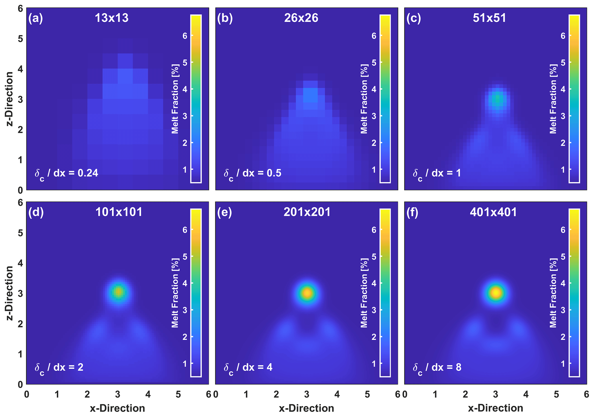
Figure 2The six panels depict a model with an initial perturbation radius of 12 times the compaction length but with different numerical grid resolutions: (a) 13×13 (b) 26×26 (c) 51×51 (d) 101×101, (e) 201×201, and (f) 401×401. The size of the compaction length in terms of grid length is given in the lower-left corner in each panel.
Figure 2 shows the resulting models for a length scale ratio of 12 for six different resolutions. The model states where φmax has risen to approximately 0.25 times the initial Stokes radius ( are shown. With increasing resolution, the maximum melt fraction increases strongly from 101×101 to 401×401 by approximately 20 %, but the velocity of φmax decreases by 7 % (not shown in the figure). Both values converge for resolutions higher than 51×51, corresponding to . Even though the compaction length is not sufficiently resolved in Fig. 2d, one can still observe the main features of the model: a main solitary wave has emerged from the original Gaussian perturbation, and secondary porosity waves are beginning to emerge within its wake. Even with , these features can be observed but are clearly underresolved. With even lower resolutions, accumulations at the top of the perturbation can be seen, which can be broadly interpreted as the attempt of a solitary wave to build up. With , the model is too coarse and the results cannot be trusted anymore.
The solitary waves modeled with our code have been compared to the semi-analytical solution of Simpson and Spiegelman (2011), and more benchmarking was carried out in Dohmen et al. (2019).
In a single-phase flow case, where the melt is not allowed to move relative to the solid, the initial perturbation ascends, shortly after beginning, with a velocity of 0.95 times the calculated Stokes velocity and then slowly decreases as the original Gauss-shaped wave deforms and loses its amplitude.
3.1 The transition from porosity wave to diapirism: Varying the initial wave radius
In this model series we vary the initial wave radius to cover the transition from porosity waves towards diapirism. As a reminder, due to our scaling the initial wave has always the same size with respect to the model box, and “increasing the initial wave radius” is equivalent to decreasing the compaction length or the size of the emerging solitary waves with respect to the model box. In Fig. 3, the models are shown at . For small radii (, a single porosity wave emerges from the original perturbation. The melt that is not situated within the emerging wave is left behind and has (for the most part) already left the model region. For , the emerged solitary wave is about the size of the initial perturbation, and even smaller radii would lead to too big waves that would not fit into the model. With increasing radius, the emerging solitary wave gets smaller. With , the resulting wave only has a size that is ∼ 20 % of the initial perturbation size.
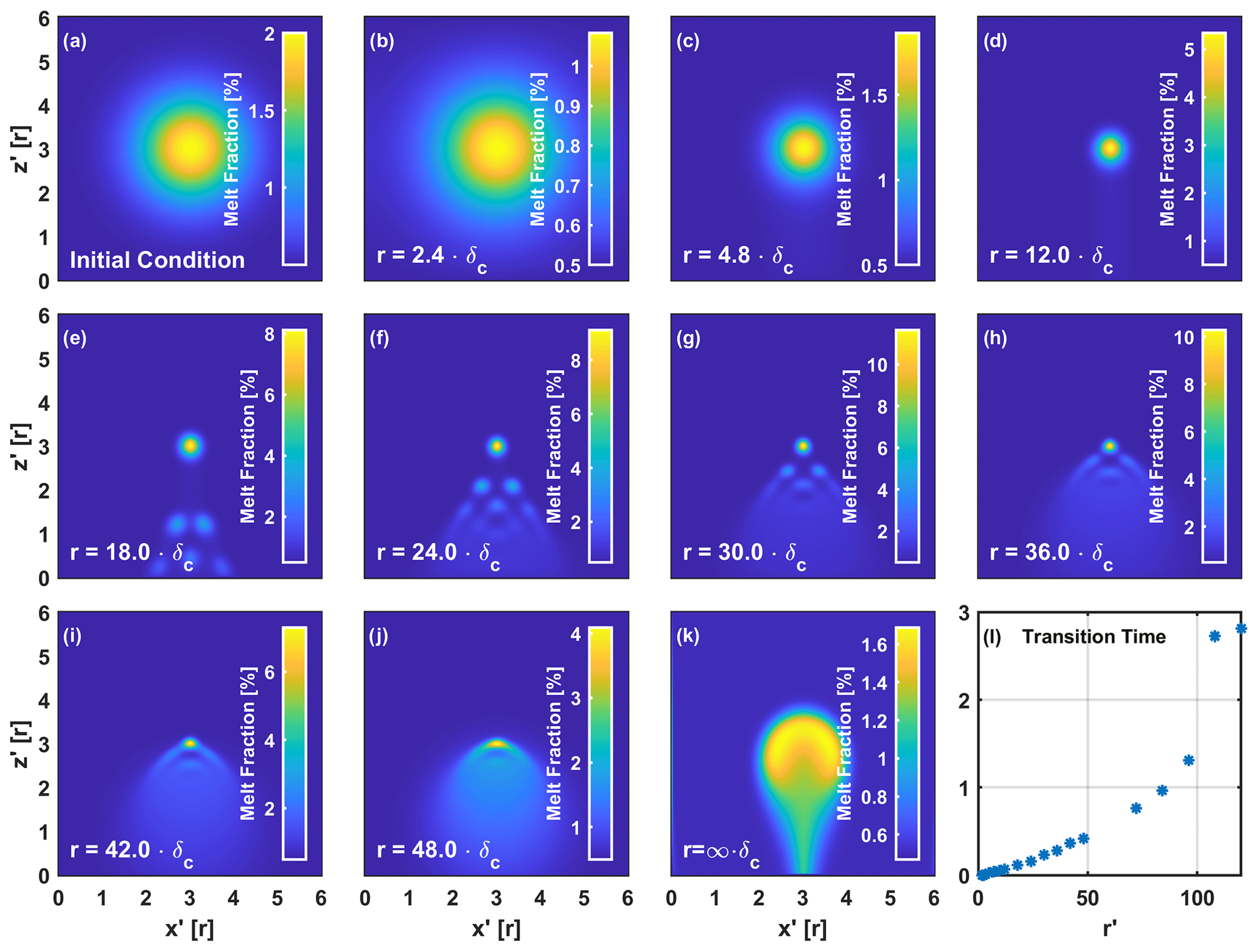
Figure 3Melt ascent morphology as function of initial perturbation radius in terms of compaction length. (a) Initial conditions of the model are valid for all cases apart of the change in compaction length. (b–j) Melt fraction distribution after for length scale ratios varying between 2.4 and 48. (k) Diapiric rise resulting from a compaction length of zero at . (l) Model transition time as a function of length scale ratios varying between 1.8 and 120. The transition time gives the time after which the main wave has reached solitary-wave status.
We compare the observed solitary-wave velocities of Fig. 3b–e to equivalent Stokes velocities for a diapir based on Eq. (16). While the dimensional Stokes velocity of a porosity anomaly is proportional to the amplitude of porosity and the square of the radius, the non-dimensional Stokes velocity is always equal to 1. In Fig. 4, this non-dimensional Stokes velocity is indicated by the dashed line with the value 1. The colored lines give 2D solitary-wave velocities with their appropriate radii, given by Simpson and Spiegelman (2011), normalized by the Stokes velocity corresponding to different initial perturbation radii. These semi-analytical solutions are in good agreement with our solitary-wave models and differ only by 3 %–5 % percent in velocity, as already shown in Dohmen et al. (2019). The velocities in this figure correspond to ratios of solitary-wave velocity to initial perturbation Stokes velocity. Inspection of Fig. 4 reveals that for the first four cases of Fig. 3b–e with radii smaller than or equal to 12⋅δc, the phase velocities are always larger than the Stokes velocity. For example, for , an emerging solitary wave with a typical radius of 4.5⋅δc has a higher phase velocity than a melt anomaly rising by Stokes flow. Thus, the cases are always in the solitary-wave regime.
For greater radii (e.g., , Fig. 3e–g) the phase velocities of solitary waves are of the order of the Stokes velocity (see Fig. 4), and they therefore need more time to separate from the remaining melt of the initial perturbation, still rising with the order of the Stokes velocity. The amount of melt accommodated within the main solitary wave is just a small percentage of the original perturbation, and secondary waves evolve in its remains. With further ascending, more and more solitary waves build up, and the former perturbation will sooner or later consist of solitary waves in an ordered cluster or a formation. This formation elongates during ascent as the main wave has a larger amplitude than all of the following waves, whose amplitudes are also decreasing with depth, as a higher proportion of melt accumulated at the top of the perturbation. Similar formations of strongly elongated fingers can be also observed in 3D, as shown by Räss et al. (2019), who used decompaction weakening. In the models with smaller radii, the main solitary wave consisted of the majority of melt originally situated within the perturbation, and just few or none secondary waves are able to emerge. With increasing radius, more melt is left behind, which allows for second and higher generations of solitary waves.
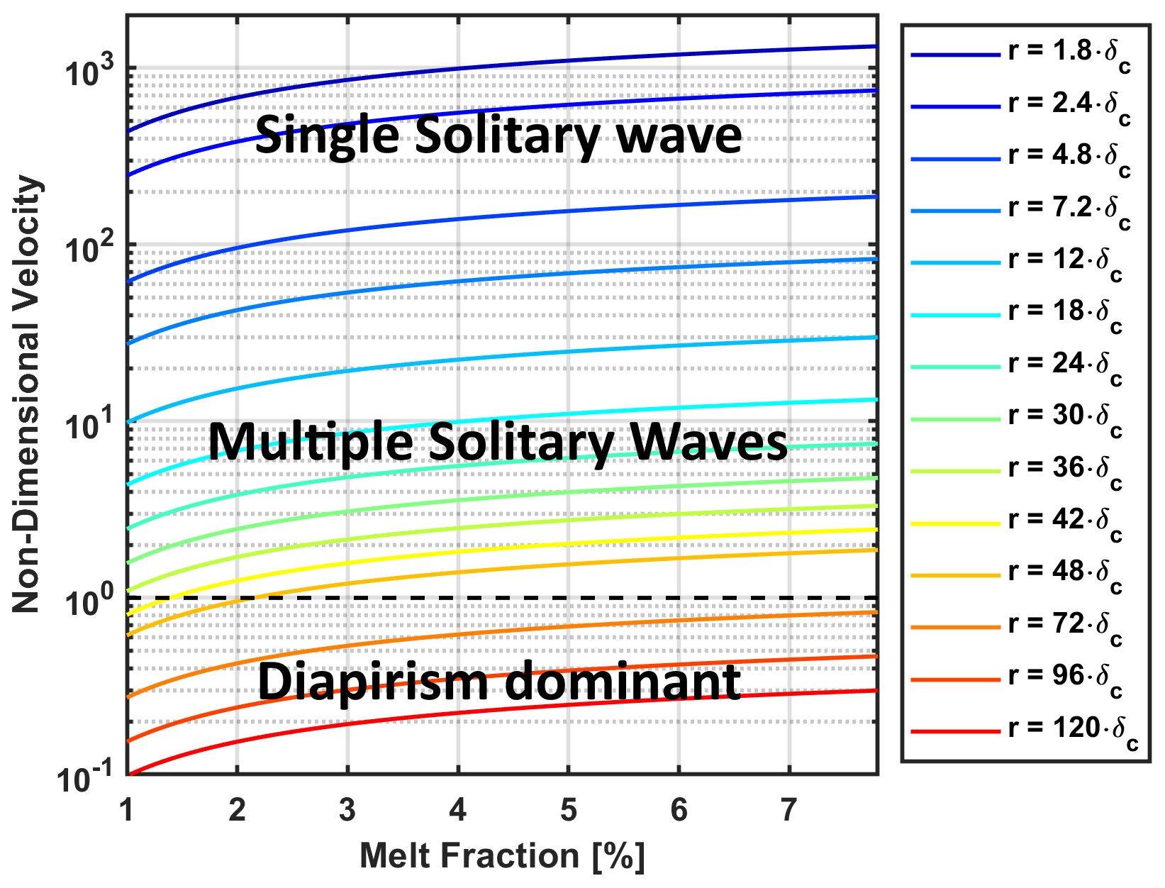
Figure 4The dashed line marks the velocity of the Stokes sphere (. The colored lines refer to the velocity of a 2D solitary wave, calculated semi-analytically by Simpson and Spiegelman (2011), in our non-dimensionalization, based on the radii shown in the legend.
For greater radii (e.g., , Fig. 3f–j), the phase velocities of solitary waves are almost equal to the Stokes velocity (See Fig. 4). This leads to almost no separation after . While for a solitary wave has already built up and is rising just ahead of the perturbation, for and just the accumulation of melt at the top of the perturbation can be observed, which will eventually lead to a solitary wave. Secondary waves also build up with higher run times, as can already be seen for .
For even greater radii, the compaction length cannot be sufficiently resolved with our approach, but tests using models that are not sufficiently resolved have shown that solitary waves can be observed for . At some point they no longer appear, probably due to lack of sufficient resolution, but our tests show that solitary waves should always emerge, even if its phase velocity is way below the Stokes velocity. As long as the ascending time is long enough and melt is able, independent of segregation velocity, to move separately to the matrix, a diapir will evolve into a swarm of a certain number of solitary waves based on the compaction length. Because the phase velocities of each small solitary wave are small compared to the Stokes velocity of the full swarm, we consider such a rising formation of melt a large-scale diapir.
Figure 3l shows the required time for the initial perturbation to build up a solitary wave. This status is achieved after the dispersion relation of the main wave reaches a point from where it follows the solitary wave dispersion relation. This time increases nearly linearly for small radii ( but increases nonlinearly for greater radii. This might be due to lack of proper resolution, but a nonlinear trend can be already observed for small radii. The transition time for radii smaller than 30⋅δc is smaller than 0.2, the time at which the models in Fig. 3b–j are shown. The other models already show solitary-wave-like blobs but did not yet reach their final form.
A classical diapir will evolve only in cases with zero compaction length (, i.e., melt is not able to move with respect to the matrix (Fig. 3k). Here, no focusing into solitary waves can be observed and transition time is infinity.
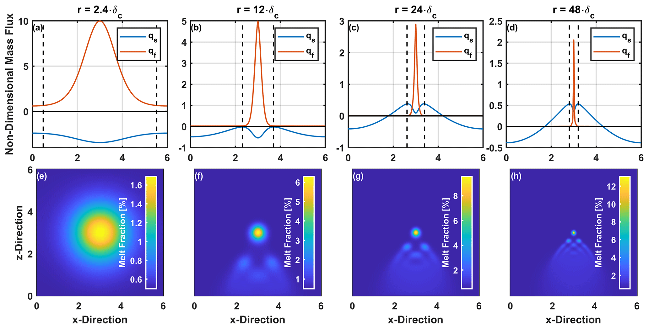
Figure 5The upper row depicts the solid and fluid mass fluxes of a horizontal line cutting through the maximum melt fraction at time steps where the main wave has just reached the status of a solitary wave. These time steps are , 0068, 0155, and 0416 from left to right, respectively. The bottom row depicts the corresponding melt porosity fields. All quantities shown are non-dimensional.
Summarizing Fig. 4, the comparison of Stokes and porosity wave velocities explains our observations shown in Fig. 3 well. For small initial radii the solitary wave velocity is clearly higher and will therefore build up and separate from the melt left behind quickly. For cases with approximately equal perturbation to solitary-wave radius only one solitary wave will build up, which includes most of the melt of the initial perturbation. With increasing perturbation radius, the velocity ratio decreases and multiple solitary waves, requiring more time, will emerge, each including only a fraction of the melt originally situated in the initial perturbation. However, even with velocity ratios smaller than 1, solitary waves emerge and, not being able to separate, rise just ahead of the remains, slowly elongating the initial perturbation.
3.2 Effects on the mass flux
It is important to study the partitioning between rising melt and solid mass fluxes in partially molten magmatic systems because melts and solids are carriers of different chemical components. Within our Boussinesq approximation, we may neglect the density differences between solid and melt. Thus, our models allow the evaluation of vertical mass fluxes of solid or fluid by quantifying the vertical velocity components multiplied with the melt or solid fractions, respectively:
Horizontal profiles of the mass fluxes through rising melt bodies are calculated at the vertical positions of maximum melt fraction at time steps where the main wave has just reached the status of a solitary wave (Fig. 5).
The mass fluxes of solid and fluid are strongly affected by the change of the initial radius from the solitary-wave regime towards the diapiric regime. For , where we observe a solitary wave, the fluid has its peak mass flux in the middle of the wave and the solid is going downwards, i.e., against the phase velocity. In the center, the fluid flux is about 10 times higher than the solid net flux. The upward flow in the center is balanced by the matrix-dominated downward flow inside and outside the wave. For , the wave area is much smaller and the ratio between solid and fluid flux is still around the order of 10. At the boundary of the wave, the solid is nearly not moving at all, but a minimum can be observed within the center of it. For , the solid flux is just above zero in the center and increases to a maximum towards the flanks of the wave that is still about 10 times smaller than the maximum fluid flux.
With , the solid flux is about 3 times smaller than the fluid flux, but most of the material ascent is accomplished by the solid. This suggests that diapiric rise begins to dominate.
The transition from solitary waves towards diapirism on qualitative model observations has so far only been based on observations. We now invoke a more quantitative criterion. In a horizontal line passing through the anomaly's porosity maximum, we define the total vertical mass flux of the rising magma body by , where the integration is carried out only in the region of increased porosity φ>φ0. This mass flux is partitioned between the fluid mass flux, , and the solid mass flux, . With these we define the partition coefficients
and
The sum Csoli+Cdia is always 1, and if Csoli>Cdia, then the solitary wave proportion is dominant, while for Csoli<Cdia diapirism is dominant. In Fig. 6a these partition coefficients for several initial radii are shown. In red the diapir is shown, and in blue the solitary wave partition coefficients are shown.
For , Csoli is equal to 5 and Cdia is equal to −4, i.e., we have a downward solid flux. With increasing radius, Cdia increases until it changes its sign and the matrix flows upward, at . It eventually becomes bigger than Csoli at and then approaches 1 for bigger radii. Csoli changes so that the sum of both is always equal to 1. Even though diapirism is dominant for , we still observe solitary waves, yet their phase velocities are much smaller than the large-scale rising velocities of the full melt formation.
The ratio of maximum fluid velocity (i.e., vf) to absolute matrix velocity (Fig. 6b) shows that for small radii, where Csoli≫Cdia, this ratio is approximately constant with a high value of about 100. The absolute velocity maxima themselves are not constant but decrease with the same rate until the switch of negative to positive matrix mass flux, where the absolute matrix velocity starts to increase, while the fluid velocity keeps decreasing. At this zero crossing we would expect a ratio of infinity, but while the zero crossing takes place within the center of the solitary wave, other regions near the wave still have finite vertical velocities. This switch from negative to positive mass flux was already observed by Scott (1988), but while they changed the viscosity ratio as an independent constant model parameter, we change the radius and keep the viscosity law the same while still evolving with φ. Both describe the transition from a two-phase limit towards the Stokes limit, but in our formulation we are able to reach the Stokes limit, whereas Scott's formulation (1988) is restricted to two-phase flow. With even greater radii the velocity ratio will eventually converge towards 1, where melt is no longer able to move relatively to the matrix (i.e., vf=vs), and material will be transported collectively as in single-phase flow. These last models are not sufficiently resolved to obtain leading and secondary solitary waves but still show the expected behavior in terms of macroscopically rising partially molten diapir.

Figure 6Quantitative parameters as function of initial perturbation radius in terms of compaction length. (a) Solitary wave (blue) and diapir (red) partition coefficients for several initial perturbation radii. (b) Ratio of maximum fluid velocity to maximum absolute solid velocity in the entire model.
Based on these observations, the evolution of these models can be divided into three regimes. (i) In the solitary wave regime ( is larger than Cdia, and the initial perturbation emerges into waves that have the properties of solitary waves and ascend with constant velocity and staying in shape. This regime can be further divided into (ia) (, where the solid mass flux is negative, and (ib) (, where the solid moves upwards with the melt. Waves in these regimes are very similar, but the further we are in regime (ia), the fewer solitary waves will emerge out of the initial perturbation. For radii smaller than about 4.8⋅δc only one wave will merge. In regime (ib) the perturbation will always emerge into multiple solitary waves.
In the diapirism-dominated regime of (ii) (, Cdia is larger than Csoli, but as the fluid melt is still able to move relatively to the solid matrix, solitary waves build up and the whole partially molten region will evolve into a swarm of them. The phase velocities of these waves are very small compared to the Stokes velocity of the perturbation and the whole swarm will rise as a diapir, whose buoyancy is still comparable to the buoyancy of the initial perturbation.
The endmember of the second regime can be reached by prohibiting the relative movement of fluid ( for which the compaction length has not to be sufficiently resolved. In this regime the initial perturbation will not disintegrate into solitary waves but instead will rise as a well-formed partially molten diapir. In every other case in the present model where fluid is able to move with respect to the solid, at some point all diapirs will evolve into a swarm of solitary waves that can be infinitely small compared to the initial perturbation. However, this is expected to happen only after a long distance of diapiric rise. In cases where the size of solitary waves is comparable to the perturbation (e.g., regime i) this will occur sooner, and in cases where solitary waves are much smaller this will occur later. Their observation is mostly limited by resolution. For models that allow for the diapir to grow (e.g., Keller et al., 2013), they may not dissolve into solitary waves as they approach the single-phase limit.
4.1 Application to nature
While in our models the perturbation size in terms of compaction lengths was systematically varied but kept constant within in each model, our results might also be applicable to natural cases in which the compaction length varies vertically. In the case of compaction length decreasing with ascent, a porosity anomaly might start rising as a solitary wave, but it may at some point enter the second regime where diapiric rise is dominant. If this boundary is sharp, the solitary wave might disintegrate into several smaller solitary waves that rise as a diapiric swarm. If the boundary is a continuous transition, the wave should slowly shrink and become slower. The melt left behind might also evolve into secondary solitary waves.
A decreasing compaction length could be accomplished by decreasing the matrix viscosity or the permeability or by increasing the fluid viscosity. Decreasing matrix viscosity might be explainable by, for example, local heterogeneities, temperature anomalies due to secondary convective overturns in the asthenosphere, or a vertical gradient of water content, which may be the result of melt-segregation-aided volatile enrichment at shallow depths in magmatic systems. This could lead to the propagation of magma-filled cracks (Rubin, 1995), as already pointed out in Connolly and Podladchikov (1998). The latter authors have looked at the effects of rheology on compaction-driven fluid flow and had similar results for an upward weakening scenario. A decrease in permeability due to a decrease in background porosity might be an alternative explanation. In the hypothetical case of a porosity wave reaching the top of partially molten region within the Earth's upper mantle or lower crust, the background porosity might decrease, which would most certainly lead to focusing because the compaction length will decrease, and eventually, when reaching melt-free rocks, the solitary waves might be small enough and have a high enough amplitude to trigger the initiation of dikes.
Even though most diapirs should, according to our models, disintegrate into numerous solitary waves, not all will inevitably do so. Within regime (i), solitary waves are possible and most probably expected, but the deeper we are in regime (ii) the less expected the disintegration is because a long time is needed for it to build up. In nature, in contrast with our models, they cannot rise for an infinite amount of time. The time needed to build up a solitary wave increases nonlinearly with r (see Fig. 3l). For example, while for a solitary wave is completely evolved after , for it needs until , i.e., equivalent to the diapiric rise time necessary to ascend the distance of approximately half the initial radii. Additionally, as already pointed out, if a model setup allows for the diapir to grow, it could approach the single-phase flow, prohibiting the emergence of solitary waves (see Keller et al., 2013).
4.2 Model limitations
The introduced partition coefficients help to distinguish whether solitary-wave or diapiric rise is dominant but cannot be solely consulted as to whether a solitary wave or a diapir can be expected. As the fluid velocity and flux are still very high in the wave center for diapiric-dominant cases, small solitary waves will build up. However, the net mass flux is dominated by the large-scale rising solid, and the formation time of small solitary waves might be long. Additionally, the internal circulation of diapirs can be faster than the phase velocity, which would smear out the emergence of solitary waves and would not allow for them to emerge. Due to the limitations of our model, we are not able to reach regions where solitary waves are small enough and their phase velocity slow enough to observe this.
While the minimum size of solitary waves in nature might be in some way limited by the grain size, in numerical models the minimum size is limited by the model's resolution. We restrict our models in this study to cases where the compaction length is at least resolved by three grid lengths dx (i.e., to get fairly resolved solitary waves, but they can be also observed for compaction lengths that are resolved much more poorly. The resolution test (Fig. 2) shows that, even though they are not solved decently, probable solitary waves can be observed for cases with δc=dx. Smaller resolutions can show indications of solitary waves but should not be trusted, as other tests (not shown here) with similar resolutions result in spurious channeling. For very poorly resolved compaction lengths ( for our models), no indications of solitary waves can be observed, and the partially molten perturbation ascends as a diapir. The deeper we are in regime 2, the more dominant the dynamics of diapirism are on a length scale of r compared to Darcy flow or solitary waves on the unresolved length scale of δc. Thus, two-phase flow, either Darcy flow or solitary waves, becomes negligible for r≫δc, and partially molten diapirs can be regarded as well resolved.
This work shows that, depending on the extent of a partially molten region within the Earth, the resulting ascent of melt may not only occur by solitary waves or by diapirs but instead by a composed mechanism where a diapir splits up into numerous solitary waves. Their phase velocities might become so slow that the whole swarm will ascend as a diapir, only slowly elongating due to the main solitary wave having a higher amplitude and therefore higher phase velocity than the following ones. Depending on the ratio of the melt anomaly size to the compaction length (or rather the model length scale to compaction length ratio), we can classify the ascent behavior into two different regimes using mass flux and velocity of matrix and melt: (ia + b) solitary wave a and b regimes, and the (ii) diapirism-dominated regime. In regime (ia), the matrix sinks with respect to the rising melt, and in regime (ib) the matrix also rises but only very slowly. The further we are in this regime, the fewer solitary waves will emerge out of the initial perturbation until eventually only one solitary wave will emerge. On the first order, these regimes can be explained by comparing Stokes velocity of the rising perturbation with the solitary-wave phase velocity. If the solitary-wave velocity is higher than the Stokes velocity, a solitary wave will evolve, and if it is lower it means that diapirism is dominant but that solitary waves will still build up if the ascending time is long enough. The deeper we are in regime (ii), the more time is needed to build up solitary waves and the less likely it is that they will appear in nature. The endmember regime (ii), i.e., pure diapirism, can be reached if fluid is not allowed to move separately from the matrix.
Numerical resolution plays an important role, especially around the transition of the regimes, as the compaction length may be under-resolved to allow for the emergence of solitary waves. Hence, it should be generally important for two-phase flow models to inspect whether solitary waves are expected and, if so, whether they have a major influence on the conclusions made.
The used finite-difference code, FDCON, is available on request.
JD wrote the paper and carried out all models shown within. HS helped with preparing the paper and initialized this project.
The authors declare that they have no conflict of interest.
The authors would like to thank Tobias Keller and an anonymous reviewer for their extensive and detailed reviews, which helped to greatly improve this paper.
This open-access publication was funded by the Goethe University Frankfurt.
This paper was edited by Taras Gerya and reviewed by Tobias Keller and two anonymous referees.
Aharonov, E., Whitehead, J., Kelemen, P. B., and Spiegelman, M.: Channeling instability of upwelling melt in the mantle, J. Geophys. Res., 100, 20433–20450, 1995.
Barcilon, V. and Lovera, O. M.: Solitary waves in magma dynamics, J. Fluid Mech., 204, 121–133, https://doi.org/10.1017/S0022112089001680, 1989.
Bittner, D. and Schmeling, H.: Numerical modelling of melting processes and induced diapirism in the lower crust, Geophys. J. Int., 123, 59–70, 1995.
Collins, W. J.: Polydiapirism of the Archean Mount Edgar Batholith, Pilbara Block, Western Australia, Precambrian Res., 43, 41–62, 1989.
Connolly, J. A. D.: Devolatilization-generated fluid pressure and deformation-propagated fluid flow during prograde regional metamorphism, J. Geophys. Res.-Sol. Ea., 102, 18149–18173, 1997.
Connolly, J. A. D. and Podladchikov, Y. Y.: Compaction-driven fluid flow in viscoelastic rock, Geodin. Acta, 11, 55–84, https://doi.org/10.1080/09853111.1998.11105311, 1998.
Connolly, J. A. D. and Podladchikov, Y. Y.: A hydromechanical model for lower crustal fluid flow, in: Metasomatism and the chemical transformation of rock, Springer, Berlin, Heidelberg, Germany, 599–658, 2013.
Connolly, J. A. D. and Podladchikov, Y. Y.: An analytical solution for solitary porosity waves: Dynamic permeability and fluidization of nonlinear viscous and viscoplastic rock, Geofluids, 15, 269–292, https://doi.org/10.1111/gfl.12110, 2015.
Costa, A.: Permeability-porosity relationship: A reexamination of the Kozeny-Carman equation based on a fractal pore-space geometry assumption, Geophys. Res. Lett., 33, L02318, https://doi.org/10.1029/2005GL025134, 2006.
Dohmen, J., Schmeling, H., and Kruse, J. P.: The effect of effective rock viscosity on 2-D magmatic porosity waves, Solid Earth, 10, 2103–2113, https://doi.org/10.5194/se-10-2103-2019, 2019.
Golabek, G. J., Schmeling, H., and Tackley, P. J.: Earth's core formation aided by flow channelling instabilities induced by iron diapirs, Earth Planet. Sc. Lett., 271, 24–33, 2008.
Griffiths, R. W.: The differing effects of compositional and thermal buoyancies on the evolution of mantle diapirs, Phys. Earth Planet. In., 43, 261–273, 1986.
Jordan, J. S., Hesse, M. A., and Rudge, J. F.: On mass transport in porosity waves, Earth Planet. Sc. Lett., 485, 65–78, https://doi.org/10.1016/j.epsl.2017.12.024, 2018.
Katz, R.: Magma dynamics with enthalpy method: Benchmark solutions and magmatic focusing ad mid-ocean ridges, J. Petrol., 49, 2099–2121, 2008.
Keller, T., May, D. A., and Kaus, B. J.: Numerical modelling of magma dynamics coupled to tectonic deformation of lithosphere and crust, Geophys. J. Int., 195, 1406–1442, 2013.
Keller, T., Katz, R. F., and Hirschmann, M.: Volatiles beneath mid-ocean ridges: Depp melting, channelized transport, focusing, and metasomatism, Earth Planet. Sc. Lett., 464, 55–68, 2017.
McKenzie, D.: The generation and compaction of partially molten rock, J. Petrol., 25, 713–765, https://doi.org/10.1093/petrology/25.3.713, 1984.
Omlin, S., Malvoisin, B., and Podladchikov, Y. Y.: Pore Fluid Extraction by Reactive Solitary Waves in 3-D, Geophys. Res. Lett., 44, 9267–9275, https://doi.org/10.1002/2017GL074293, 2017.
Popov, A. A. and Sobiolev, S. V.: SLIM3D: A tool for three-dimensonal thermomechanical modeling of lithospheric deformation with elasto-visco-plastic rheology, Phys. Earth Planet. In., 171, 55–75, 2008.
Rabinowicz, M., Ceuleneer, G., and Nicolas, A.: Melt segregation and flow in mantle diapirs below spreading centers: Evidence from the Oman Ophiolite, J. Geophys. Res.-Sol. Ea., 92, 3475–3486, https://doi.org/10.1029/jb092ib05p03475, 1987.
Räss, L., Duretz, T., and Podladchikov, Y. Y.: Resolving hydromechanical coupling in two and three dimensions: Spontaneous channelling of porous fluids owing to decompaction weakening, Geophys. J. Int., 218, 1591–1616, https://doi.org/10.1093/gji/ggz239, 2019.
Richard, G. C., Kanjilal, S., and Schmeling, H.: Solitary-waves in geophysical two-phase viscous media: A semi-analytical solution, Phys. Earth Planet. In., 198–199, 61–66, https://doi.org/10.1016/j.pepi.2012.03.001, 2012.
Richardson, C. N.: Melt flow in a variable viscosity matrix, Geophys. Res. Lett., 25, 1099–1102, 1998.
Rivalta, E., Taisne, B., Bunger, A. P., and Katz, R. F.: A review of mechanical models of dike propagation: Schools of thought, results and future directions, Tectonophysics, 638, 1–42, 2015.
Rubin, A. M.: Propagation of magma-filled cracks, Annu. Rev. Earth Pl. Sc., 23, 287–336, https://doi.org/10.1146/annurev.ea.23.050195.001443, 1995.
Schmeling, H.: Partial melting and melt segregation in a convecting mantle, in: Physics and Chemistry of Partially Molten Rocks, Springer, Dordrecht, The Netherlands 141–178, 2000.
Schmeling, H., Marquart, G., Weinberg, R., and Wallner, H.: Modelling melting and melt segregation by two-phase flow: New insights into the dynamics of magmatic systems in the continental crust, Geophys. J. Int., 217, 422–450, https://doi.org/10.1093/gji/ggz029, 2019.
Scott, D. R.: The competition between percolation and circulation in a deformable porous medium, J. Geophys. Res.-Sol. Ea., 93, 6451–6462, https://doi.org/10.1029/JB093iB06p06451, 1988
Scott, D. R. and Stevenson, D. J.: Magma solitons, Geophys. Res. Lett., 11, 1161–1164, 1984.
Simpson, G. and Spiegelman, M.: Solitary wave benchmarks in magma dynamics, J. Sci. Comput., 49, 268–290, https://doi.org/10.1007/s10915-011-9461-y, 2011.
Slezkin, A.: Dynamics of viscous incompressible fluid, Gostekhizdat, Moscow, Russia, 1955 (in Russian).
Sparks, D. and Parmentier, E.: Melt extraction from the mantle beneath spread-ing centers, Earth Planet. Sc. Lett., 105, 368–377, https://doi.org/10.1016/0012-821X(91)90178-K, 1991.
Spiegelman, M.: Physics of Melt Extraction: Theory, Implications and Applications, Philos. T. Roy. Soc. A, 342, 23–41, https://doi.org/10.1098/rsta.1993.0002, 1993a.
Spiegelman, M.: Flow in deformable porous media, Part 2 Numerical analysis – the relationship between shock waves and solitary waves, J. Fluid Mech., 247, 39–63, https://doi.org/10.1017/S0022112093000370, 1993b.
Spiegelman, M. and McKenzie, D.: Simple 2-D models for melt extraction at mid-ocean ridges and island arcs, Earth Planet. Sc. Lett., 83, 137–152, 1987.
Šrámek, O., Ricard, Y., and Dubuffet, F.: A multiphase model of core formation, Geophys. J. Int., 181, 198–220, 2010.
Stevenson, D. J.: Spontaneous small-scale melt segregation in partial melts undergoing deformation, Geophys. Res. Lett., 16, 1067–1070, 1989.
Turcotte, D. L. and Schubert, G.: Geodynamics, Cambridge University Press, New York, 287–292 and 298–303, 1982.
Watson, S. and Spiegelman, M.: Geochemical Effects of Magmatic Solitary Waves – I. Numerical Results, Geophys. J. Int., 117, 284–295, https://doi.org/10.1111/j.1365-246X.1994.tb03932.x, 1994.
Wiggins, C. and Spiegelman, M.: Magma migration and magmatic solitary waves in 3D, Geophys. Res. Lett., 22, 1289–1292, https://doi.org/10.1029/95GL00269, 1995.
Yarushina, V. M., Podladchikov, Y. Y., and Connolly, J. A. D.: (De)compaction waves in porous viscoelastoplastic media: Solitary porosity waves, J. Geophys. Res.-Sol. Ea., 120, 4843–4862, https://doi.org/10.1002/2014JB011260, 2015.