Comparing global seismic tomography models using varimax principal component analysis

Global seismic tomography has greatly progressed in the past decades, with many global Earth models being produced by different research groups. Objective, statistical methods are crucial for the quantitative interpretation of the large amount of information encapsulated by the models and for unbiased model comparisons. Here we propose using a rotated version of principal component analysis (PCA) to compress the information in order to ease the geological interpretation and model comparison. The method generates between 7 and 15 principal components (PCs) for each of the seven tested global tomography models, capturing more than 97 % of the total variance of the model. Each PC consists of a vertical profile, with which a horizontal pattern is associated by projection. The depth profiles and the horizontal patterns enable examining the key characteristics of the main components of the models. Most of the information in the models is associated with a few features: large low-shear-velocity provinces (LLSVPs) in the lowermost mantle, subduction signals and low-velocity anomalies likely associated with mantle plumes in the upper and lower mantle, and ridges and cratons in the uppermost mantle. Importantly, all models highlight several independent components in the lower mantle that make between 36 % and 69 % of the total variance, depending on the model, which suggests that the lower mantle is more complex than traditionally assumed. Overall, we find that varimax PCA is a useful additional tool for the quantitative comparison and interpretation of tomography models.

1 Introduction

Global seismic tomography has brought a new understanding of the current state of the mantle through the inversion of massive seismic datasets to build 3-D images of the Earth's interior of both isotropic and anisotropic structure, the latter being one of the most direct ways to constrain mantle flow (e.g. Rawlinson et al., 2014; Chang et al., 2014; McNamara, 2019). The interpretation and comparison of tomography models often include computing correlations between two models with depth and degree, analysing power spectra (e.g. Becker and Boschi, 2002), and visual inspections and qualitative or simple descriptions of the retrieved patterns, for example of subducted slab or mantle plume candidates (e.g. Auer et al., 2014; French and Romanowicz, 2014; Chang et al., 2016; Ferreira et al., 2019). While the large-scale upper mantle and lowermost mantle isotropic structure is fairly consistent from one model to the other, discrepancies appear when considering small-scale structures. Moreover, there are substantial differences between existing global anisotropy models (e.g. Chang et al., 2014; Romanowicz and Wenk, 2017). Nowadays, codes or web-based tools facilitate the interpretation and visual comparison of different models (e.g. Durand et al., 2018; Hosseini et al., 2018). This allows for the identification of regions with good agreement between seismic models using e.g. vote maps (Lekic et al., 2012) or through statistical tools showing the relative frequency of seismic anomalies at specific depth ranges (Hosseini et al., 2018). However, the large amount of information encapsulated in global tomography models, which typically involve tens of thousands of model parameters, can be difficult to mine and interpret efficiently.

Statistical methods used in other disciplines to analyse and classify big data and models may be useful to further enhance the analysis of seismic tomography models by providing a common ground for comparison. For example, in recent years, clustering methods have been used to partition seismic tomography models into groups of similar velocity profiles, providing an objective way of comparing the models (Lekic et al., 2012; Cottaar and Lekic, 2016). Here, we propose implementing principal component analysis (PCA; von Storch and Zwiers, 1999) to substantiate and clarify what can be learn from such comparisons, as recently proposed by Ritsema and Lekić (2020). The PCA-based method aims at approximating the tomographic models by a sum of a given number $\stackrel{\mathrm{̃}}{N}$ of components, with $\stackrel{\mathrm{̃}}{N}$ smaller than the actual number of slices. Each PC consists of a vertical profile, which is the principal component (PC), and a horizontal pattern, which is the load. Most of the variance of the signal being captured by a reduced number of PCs allows us to grab all the information by analysing only the relevant components resulting from an efficient compression.

Although the first PC, capturing the largest variance, often corresponds to an actual physical process, the others are increasingly difficult to interpret. The physical interpretation of the PCs and loads can be made easier by redistributing PCA components along other eigenvectors. We propose applying the varimax criterion (Kaiser, 1958) that allows focusing on PCs with large values concentrated on the smallest possible subset of depths, as it is physically likely that mantle structures have a limited depth extension rather than spanning over the whole mantle depth. Previous studies in other fields of Earth sciences (see e.g. the thorough review paper by Richman, 1986) showed that, when using the varimax criterion, the redistributed components are often less sensitive to computation artefacts, for example related to data geometry, while keeping the same degree of compression as the original PCs.

Varimax analysis has previously been successfully used in various applications, such as to analyse climate models, whereby the different models are projected on the same set of PCs, allowing a direct comparison in terms of captured variance and retrieved features (Horel, 1981; Sengupta and Boyle, 1998; von Storch and Zwiers, 1999; Tao et al., 2019; Kawamura, 1994). Motivated by these successful results, we apply varimax PCA to the interpretation and comparison of global tomography models. Note that we do not propose using the varimax method as an alternative Earth model representation to the model solutions from which they are derived. Instead, we propose it as a diagnostic tool, allowing for the quantification of the level of independent information in the tomography models and an easier comparison of the models. Projecting the models on a set of independent vertical profiles provides an optimal representation for a given number of slices (number of components) smaller than the original number of splines and boxes or for a given portion of the information present in the model (captured variance).

In Sect. 2, we present the seven global tomography models used, followed by a description of the statistical methods used in this study. Then, in Sect. 4 we compare classical and varimax PCA with a k-means clustering approach. Sections 5–6 present and discuss the results from the application of varimax PCA to the seven tomography models considered. We then present a brief final discussion and conclusions in Sect. 7.

2 Seismic tomography models

We use seven 3-D global seismic tomography models: (i) S20RTS (Ritsema, 1999), (ii) S40RTS (Ritsema et al., 2011), (iii) SEISGLOB2 (Durand et al., 2017), (iv) SEMUCB-WM1 (French and Romanowicz, 2014), (v) SGLOBE-rani (Chang et al., 2015), (vi) S362WMANI+M (Moulik and Ekström, 2014) and (vii) SAVANI (Auer et al., 2014). While the first three models are isotropic shear-wave-speed models, the last four models also include lateral variations in radial anisotropy. These models were built from different datasets using distinct modelling approaches, as summarised in Table 1. We focus on shear-wave models because the agreement of P-wave models is more limited (e.g. Cottaar and Lekic, 2016). Nevertheless, future work may expand the analysis to recent P-wave models (Hosseini et al., 2020) The models used show the key features in current global isotropic and radially anisotropic models, and they are hence representative of the current state of global tomography. For example, all isotropic shear-wave-speed models show a good correlation with tectonic features in the upper mantle, such as mid-ocean ridges and cratons (see ∼  100 km in Fig. A1a). Moreover, they show the signature of subducting slabs around ∼  600 km of depth and the two prominent large low-shear-velocity provinces (LLSVPs) beneath Africa and the Pacific in the bottom of the mantle at ∼  2900 km of depth (Fig. A1a). On the other hand, the agreement between the anisotropy models is much more limited (Fig. A1b); common features between the models include a well-known positive radial anisotropy anomaly beneath the Pacific at ∼  150 km of depth, negative radial anisotropy anomalies beneath the East Pacific Rise at ∼  200 km of depth and negative radial anisotropy anomalies associated with the LLSVPs. The latter anomalies have been shown to be artefacts in the models due to the poor balance between SV- and SH-sensitive travel-time data in various existing body-wave datasets, which have much more data sensitive to SH than to SV motions (e.g. Chang et al., 2014; Kustowski et al., 2008). On the other hand, Moulik and Ekström (2014) showed that such spurious anisotropic features in even-degree structure are reduced by using self-coupling normal-mode splitting data in the inversions. Yet, trade-offs between isotropic and anisotropic structure in the lowermost mantle persist in odd-degree structure, which is not constrained by self-coupling normal-mode splitting data.

We obtained the global tomography models either directly from their authors or from the IRIS Earth model collaboration repository (REFS – http://ds.iris.edu/ds/products/emc/, last access: 12 October 2020). Since some of the models have different reference 1-D models and use distinct parameterisations, for consistency we converted them into perturbations in shear-wave speed and in radial anisotropy with respect to the 1-D model PREM (Dziewonski and Anderson, 1981) on a common grid with a $\mathrm{1}{}^{\circ }\times \mathrm{1}{}^{\circ }$ horizontal sampling and on 29 depth slices starting at 50 km of depth with a 100 km spacing from 100 to 2900 km of depth. This conversion into the same 1-D reference model eases comparison. Moreover, since both the vertical structure and the horizontal patterns are normalised, this also implies that the background model does not impact our analysis. In addition to the gridded representation allowing fair graphical presentation, we interpolate the datasets from the horizontal grids into a regular polyhedron of 9002 equi-areal faces, the vertexes of which were generated through the icosahedron tool of (Zechmann, 2019). This transformation produces a uniform sampling of the sphere, with each vertex having a surface corresponding to that of a 250×250 km² square. Considering that the statistical methods used in this study use the captured variance as a major criterion for ordering the components, the use of gridded data would overweight the contribution at the poles in the PC representation. The $\mathrm{180}\times \mathrm{360}\times \mathrm{29}$ individual model data matrices are thus converted into 9002×29 matrices. As the shallowest layers contain the majority of the variability in the velocity anomalies, most of the principal components will be captured in those layers, which will be over-represented. Hence, the shear-wave-speed and radial anisotropy perturbations are normalised by slice; i.e. the mean value of the slice is subtracted from each value, and each value is divided by the standard deviation of the slice. This is relevant, as in this study we investigate relative values on a given profile; the actual magnitude can be recovered by multiplying the load patterns by the standard deviation of the layer in the original model. The normalisation applied to the models does not lead to a loss of information.

(Chang et al., 2015)(Auer et al., 2014)(Ritsema, 1999)(Ritsema et al., 2011)(French and Romanowicz, 2014)(Moulik and Ekström, 2014)(Kustowski et al., 2008)(Durand et al., 2017)

Table 1 Global tomography models used in this study, including a short description of the data, parameterisation and the modelling approach used in their construction. All models were built using least-squares inversions with different regularisation choices.

3 Methods

Previous studies have compared global tomography models using k-means clustering (e.g. Lekic et al., 2012) or PCA (Ritsema and Lekić, 2020). Though PCA is very different in many respects from the clustering of the k-means method, it is useful to start by comparing PCA and varimax PCA results with those from the k-means for an illustrative tomography model (S40RTS).

3.1 k-means clustering

Considering the three-dimensional dataset $D({\mathit{\lambda }}_i,{\mathit{\varphi }}_i,z_j)$, the k-means algorithm (MacQueen, 1967) defines k clusters, corresponding to the k sets of horizontal positions (λ_i,ϕ_i) closest to their average z_i profiles. The algorithm is based on an iterative procedure. At the first iteration, it randomly chooses k horizontal positions used as cluster centres. Each point of the dataset is then associated with the cluster centre to which it is the closest. The average radial profile of the points attributed to each given cluster is computed and used as the new cluster centre for the next iteration. This is repeated until convergence is achieved.

To make k-means and PCA representations somewhat comparable, we use the clusters as horizontal patterns and the average vertical profiles of each cluster as the PCs. By construction, the variance captured by the k-means is noticeably smaller than that for the other methods, since it is not meant to propose a compressed representation of the dataset but rather to separate the dataset into subsets, which results in an important loss of information.

3.2 Principal component analysis (PCA)

A 2-D matrix (F_j,k, j=1, 2, …, J; k=1, 2, …, K) is transformed by the PCA into a sum of components, with each component being composed of a load α_n,j and an eigenvector A_n,k.

$$\begin{array}{}\text{(1)}& {\mathbf{F}}_{j,k}=\sum _{n=\mathrm{1}}^{N=\min (J,K)}{\mathit{\alpha }}_{n,j}{\mathit{A}}_{n,k}\end{array}$$

In our case, F_j,k corresponds to the velocity anomaly at horizontal position $p_j=({\mathit{\lambda }}_j,{\mathit{\varphi }}_j)$ and depth z_k. The A_n,k are the eigenvectors, or principal components (PCs), of the covariance matrix. These PCs are orthogonal vertical structures representing the covariance between the slices of the model. It has large positive values if the horizontal structures from two layers are positively correlated, zero values if the structures are not correlated, and large negative values if they are anticorrelated. The loading patterns α_n,j are also orthogonal to each other, and each α_i,j results from the projection of the dataset on the PC i, capturing the horizontal structure i associated with the vertical anomaly profile A_i,k. The loads take continuous positive and negative values. Here, those patterns correspond to horizontal maps showing where each vertical structure is more or less important in the model.

The components are ordered by decreasing eigenvalue, as the variance captured by each PC is directly proportional to the eigenvalue of the PC. Due to their orthogonality and to the mathematical properties of the transformation, the variance captured by each PC drops rapidly with the order so that a small number of independent components ($\stackrel{\mathrm{̃}}{N}\ll N=\mathrm{29}$) is often sufficient to capture most of the information, allowing an efficient compression of the dataset.

Unlike clustering methods, which are binary in that any horizontal location only belongs to one cluster, PCA computes the amplitude of the contribution from each principal component for every horizontal location, providing a compressed reconstruction of the dataset.

The first PC corresponds to the dominant covariance, which might be physically associated with a global phenomena – in our case, a structure that would develop on the whole mantle depth – or a more local feature, i.e. associated with a limited depth range. But this covariance structure might also correlate with other features from other depths, which will also be retrieved in the first PC. The second PC being orthogonal to the first, some of the physics might have been subtracted by the computation of the first PC, and it is even more so for the following principal components.

3.3 Varimax PCA

Used on space–time datasets, PCA often produces artefacts from the domain geometry (Richman, 1986): the topographies of the PCs are primarily determined by the shape of the domain and not by the covariation among the data. In other words, different correlation functions on a geometrically shaped domain have similar load patterns in a predictable sequence, which do not reflect the underlying covariation. This is the case of square domains found, for example, on meteorological maps; in our case, the unrotated PCs show a harmonic-like progression, with one maximum for the first PC, two for the second, and so on. In contrast, the varimax rotation captures distinct, well-defined depth domains in the mantle, which are easier to interpret physically. Hence, the physical interpretation of the PCs and load can be made easier by redistributing PCA components along other eigenvectors, thereby maximising a functional of the loads that favours some physical properties that appear physically meaningful (von Storch and Zwiers, 1999; Neuhaus and Wrigley, 1954). There are several possible redistribution options for the PCs (von Storch and Zwiers, 1999; Browne, 2001; Jolliffe, 2005). Among those, varimax rotation (Kaiser, 1958) favours PCs with large values concentrated on the smallest possible subset of depths and preserves the orthogonality of the PCs.

Varimax rotation corresponds to a rotation on the basis of the same information space as that generated by the PCA; consequently, the total variance captured by $\stackrel{\mathrm{̃}}{N}$ components is exactly the same for both types of PCs but distributed differently between the components, with a slower variance decrease for the varimax rotated solution. Considering the variance captured by the PCA components, the number $\stackrel{\mathrm{̃}}{N}$ of PCs to keep is selected to meet a given criterion: the total variance captured, a fixed number of components or the minimum variance captured by a PC kept. Then we define new $\stackrel{\mathrm{̃}}{N}$ components so that

$$\begin{array}{}\text{(2)}& {\mathbf{F}}_{j,k}\simeq \sum _{n=\mathrm{1}}^{\stackrel{\mathrm{̃}}{N}}{\mathit{\alpha }}_{n,j}{\mathit{A}}_{n,k}=\sum _{n=\mathrm{1}}^{\stackrel{\mathrm{̃}}{N}}{\mathit{\beta }}_{n,j}{\mathit{B}}_{n,k}.\end{array}$$

β_n,j represents the new horizontal structures, and the new PCs, B_n,k, are chosen to maximise a given objective function V, defined by the sum of the values of the objective functions V_n computed over each PC:

$$\begin{array}{}\text{(3)}& V=\sum _n^{\stackrel{\mathrm{̃}}{N}}{V}_n\left({\mathit{B}}_{n,k}\right),\end{array}$$

with

$$\begin{array}{}\text{(4)}& V_n={\displaystyle \frac{\mathrm{1}}{K}}\sum _{k=\mathrm{1}}^K{\left({\displaystyle \frac{{\mathit{B}}_{n,k}}{s_k}}\right)}^{\mathrm{4}}-{\displaystyle \frac{\mathrm{1}}{K^{\mathrm{2}}}}\sum _{k=\mathrm{1}}^K{\left({\displaystyle \frac{{\mathit{B}}_{n,k}}{s_k}}\right)}^{\mathrm{2}},\end{array}$$

where s_k represents normalisation factors, with s_k=1, for all k in the case of varimax rotation.

This transformation corresponds to a rotation of the PCs because the subspace generated by the transformation – or the reconstructed model – is the same as with the non-rotated PCA limited to $\stackrel{\mathrm{̃}}{N}$ components. In our case, it limits the vertical extension of the PCs; i.e. each PC shows large values on only a few depths and/or slices.

The associated horizontal structures, β_n,j, are recomputed by projection of the tomography model on the rotated vertical profile. This rotation conserves the orthogonality of the eigenvector, which is not the case for all the possible rotations, but the horizontal loads are often not orthogonal anymore (Mestas-Nuñez, 2000). The total variance captured by the rotated PCs is the same as that from unrotated PCs, but the decrease in the variance is slower than that from the original decomposition.

4 Comparing the PCA, varimax rotated PCA and k-means results for the model S40RTS

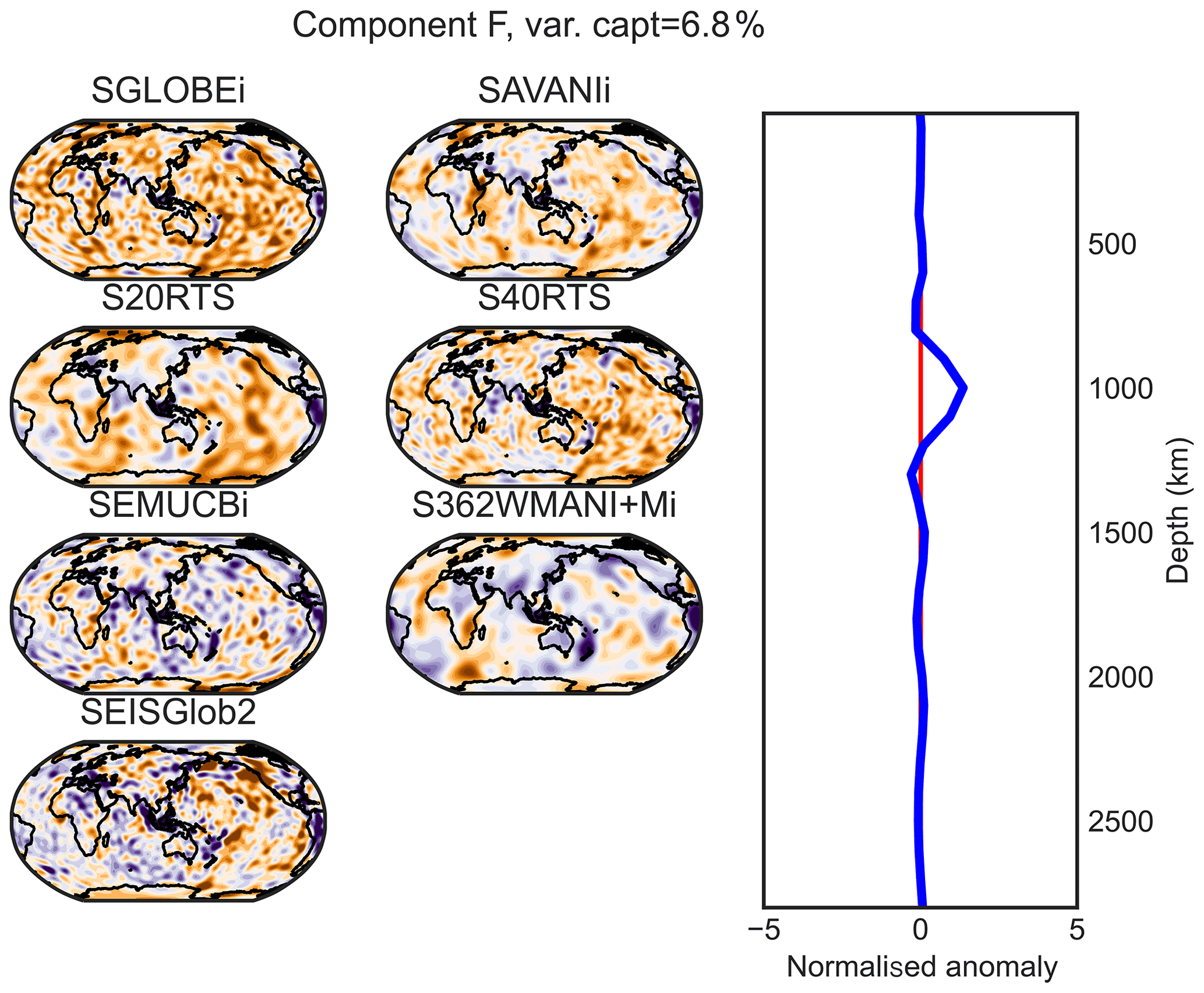
Figure 1 shows the PCs and loads resulting from the application of the PCA, varimax rotated PCA and k-means clustering methods to the tomography model S40RTS for a six-PC decomposition. All the methods are applied to the same normalised data. The x axis, i.e. the amplitude of the vertical eigenvectors, represents the maximum absolute value of the normalised anomaly at a given depth. It must be multiplied by the horizontal loading pattern, which provides normalised loads ranging between −1 and 1.

Figure 1 highlights the complementarity of the k-means and varimax PCA methods. While the k-means method allows us to highlight key large-scale features, such as the distribution of lowermost mantle velocity and to compare how it appears in the different models (e.g. Lekic et al., 2012), the varimax PCA approach provides a compressed representation of the full model. Being binary, the k-means method does not provide amplitudes; i.e. the load for each PC is either 0 or 1: every location is part of one k-means cluster, while it can be part of several PCs in the PCA. The latter inherently captures more complexity with fewer principal components than k-means clustering. Hence, it is not surprising that the six k-means components capture only 34 % of the total model variance, whereas both PC-based methods recover 83.2 % (Fig. 1). Therefore, while the k-means method is a useful classification technique that allows a subset of data to be separated out from others, varimax PCA is a distinct, valuable compression technique that reduces the number of parameters while minimising loss of information. It allows identifying the most important components of tomographic models, easing their interpretation.

As expected, the PCA profiles A_i(z) show increasingly oscillating patterns with i, which may lead to nonphysical interpretations. For example, the signature of tectonic patterns such as ridges, subduction zones and cratons spread over the whole mantle (principal components 4 and 5, purple and cyan in the top row in Fig. 1) observed in the unrotated PC representation makes no physical sense. More generally, the vertical profiles retrieved by PC analysis are certainly not all associated with sound geophysical structures. Only the first PC (red) provides directly interpretable patterns: the African and Pacific large low-shear-velocity provinces (LLSVPs) (Garnero and McNamara, 2008; McNamara, 2019), whose depth extent with a maximum below 1800 km can be nicely visualised in Fig. 1. Without normalisation, every eigenvector shows a strong contribution from the shallowest mantle (<250 km), where most of the variance is located, as in Ritsema and Lekić (2020). Indeed, due to the absence of normalisation, all four main PCs obtained by Ritsema and Lekić (2020) contain a lot of energy in the shallowest zone, while our normalisation allows keeping the tectonically driven zone in essentially two components out of six (component 4 capturing 7.6 % of the variance and component 5 capturing 6.2 %.)

On the other hand, the normalised varimax procedure recovers well-known structures. Within its first mode, we recover the tectonic patterns, and the LLSVPs gradually appear in the three last components (for a more detailed analysis, see the next section). Based on these comparisons, we find that the varimax PC method is useful to concentrate coherent information at different depths that is available in the seismic tomography models, without any preconception. The next sections will thus focus on the application of this method to the interpretation of the global tomography models considered in this study.

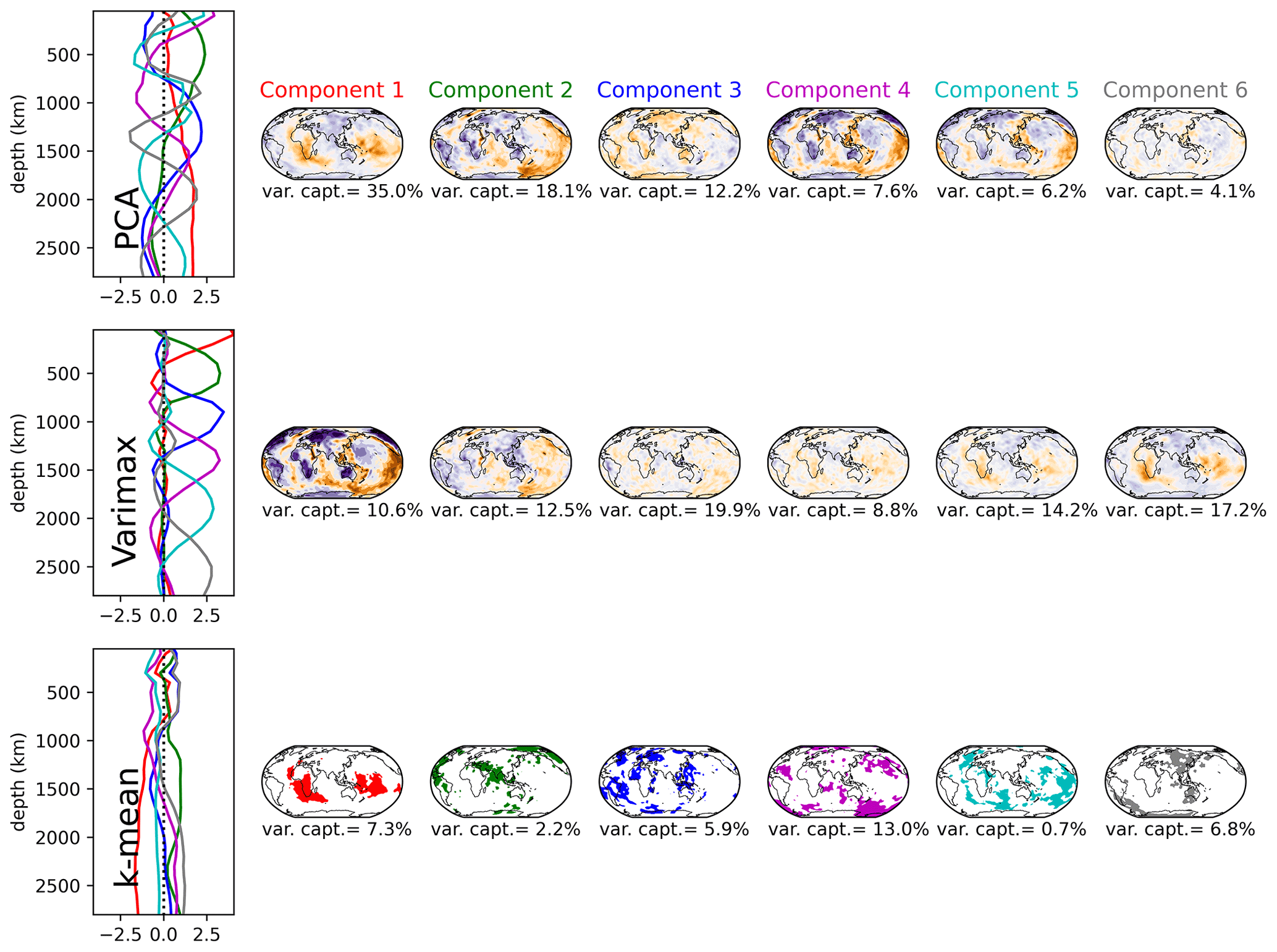
Figure 1 Results from the PC, varimax and k-means methods applied to the model S40RTS using six principal components. The varimax PC and loads are normalised in such a way that the horizontal patterns (load) range between −1 and 1, with orange corresponding to negative, blue to positive and white to zero, with the intensity being proportional to the value. We note that while this normalisation eases the analysis, it does not lead to a loss of information (see main text for details). Unlike the classical variance-based sorting of the principal components, we order the varimax components by the depth of the profile's maximum.

5 Compressed information from varimax PCA

5.1 Comparison of vertical profiles and horizontal patterns

We use varimax PCA to compress the seven tomography models described in Sect. 2 into a set of components, keeping only the most important ones, as explained below. Each component is composed of a vertical profile obtained directly from the varimax process and an associated horizontal pattern, which is computed by projecting the model on the profile. Such data compression is useful to compare the models if three major conditions hold. First, a subset of components must capture most of the variance of the signal, with the number of components being significantly smaller than the original number of depth splines and boxes, and enhance the signal-to-noise ratio. Secondly, the relevant structures in the mantle, which will be used for comparison and for geological interpretation, should not be distorted by the compression; i.e. their shape and position must remain unchanged. Third, the power spectral densities should not be altered by the compression process.

In order to facilitate the comparison of the horizontal structures in the models, we label the varimax components obtained from the varimax PCA using capital letters in alphabetical order from components sensitive to shallow mantle structure to components sensitive to the lowermost mantle structure. Figure 2 shows the variance captured by the varimax PCA applied to the different models. The varimax analysis is performed by considering all the components capturing more than 1 % of the variance of the signal in the classical PCA. Keeping only the components with variance above 1 % limits the number of maps, facilitating the quest for relevant information. Tests with 5 % and 10 % thresholds showed that some important information is lost. When using a 10 % threshold, all the models are represented by three components only, which misrepresent known structures such as ridges or subduction zones. Moreover, the depth distributions of the corresponding PCAs become quite broad and imprecise, each stretching over more than 1000 km depth ranges. In the 5 % threshold case, the models are represented by four (SAVANIi) to six components (SEMUCB−WM1i, SEISGLOB2). Again, information is lost concerning e.g. ridges or subduction zones, and the depth information is spread over a depth range greater than 500 km for all components and for all models.

The simplification brought by the varimax method is particularly efficient for tomography models with weak regularisation, such as SGLOBE-ranii, wherein short-scale structure is likely mixed with noise. Figure 2 shows that the number of varimax components ranges from 7 for model SAVANIi to 15 for SGLOBE-ranii, with the total variance captured by all these principal components always exceeding 97.3 % (see also Table 2, which summarises the components kept in the varimax analysis). The number of varimax components required by each model depends on the details of the model's construction, such as the data used (Table 1), and, importantly, on subjective choices made, such as the level of regularisation used. Increasing the strength of regularisation reduces the model's effective number of free parameters and hence the number of varimax components required by the model. As the SAVANI model only needs seven varimax PCA components, the shallowest component concentrates a lot of information (26 % of the variance) that is spread into more components for the other models. Table 2 shows that the number of PCs needed to explain 97.3 % or more of the total information in the tomography models is always smaller than the number of splines or layers used in the models' original depth parameterisation, with 29 % to 75 % fewer PCs than depth splines and layers.

This fulfils the first condition for the usefulness of the data compression mentioned above. In order to check the second condition previously mentioned, Fig. B1 compares six examples of depth slices in the original SEMUCB−WM1i model with those obtained from the model's reconstruction using varimax analysis. The differences between the original and reconstructed models are small and random, highlighting the fact that the compression process does not distort the model's features. The residual signal is the part of the models that is not covariant vertically. We also verified that there are only very small, random differences between the power spectra of the original and the reconstructed models (see Figs. B2 and B3 in the Appendix). Hence, the third condition of usefulness of the data compression used in this study is also satisfied.

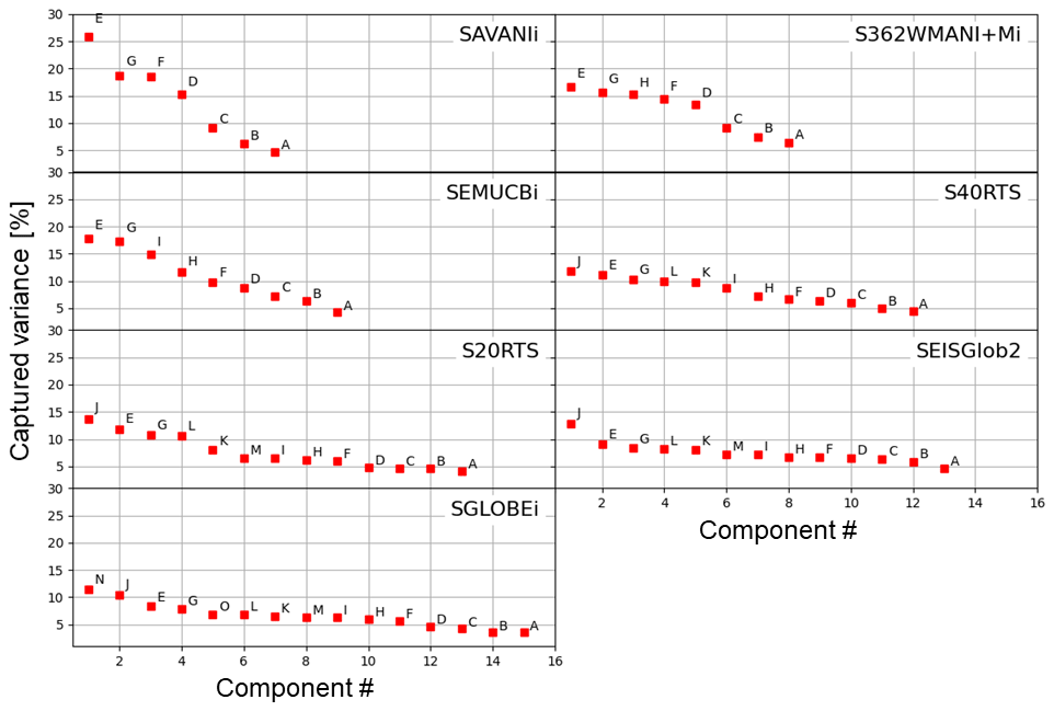
Figure 2 Captured variance by the PC varimax method, applied to the isotropic part of the seven tomography models used in this study. The number of components is chosen such that during the PCA, we only keep the components explaining more than 1 % of the variance, which occurs after 7 (SAVANIi) to 15 (SGLOBE-ranii) components. The varimax PCs are sorted alphabetically from the shallowest one to the deepest ones.

Figure 3 Principal components for the different individual model varimax PCAs and the combined one (see Sect. 6) for the isotropic part of the seven tomography models used in this study. Only the PC components above 1 % are kept in this analysis (Fig. 2). The dashed grey lines represent the spline functions and the grey boxes the variable thickness depth layers used by the different models. The vertical dashed lines indicate the 410 and 660 km seismic discontinuities.

Figure 3 shows the varimax PCs for all the tomography models used in this study, together with the spline functions or the variable thickness depth layers used in the models' parameterisation. The vertical profiles differ from one model to the other in both numbers of components and the depths of their maxima. For example, as shown in Fig. 2, SAVANIi requires 7 components, while SGLOBE-ranii needs 15 components. We re-emphasise that the number of principal components obtained for a given model reflects their amount of independent information, which in turn depends heavily on choices made during the model's construction, such as regularisation and the amount and type of data used.

The horizontal patterns obtained from the varimax PCA also show distinct features, but this is not always in the same way as for the vertical profiles (Figs. 4, C1–C6). S20RTS shows sharp vertical profiles (Fig. C3) and even contains one more PC (13) in the upper mantle than the updated S40RTS model (12, Fig. C4), but the horizontal patterns are smoother. This is likely due to the fact that the latter model is constrained by about 10 times more data and used a different level of regularisation (Ritsema et al., 2011). SGLOBE-ranii, SEMUCB−WM1i and SEISGLOB2 (Figs. C1, 4 and C6) depict sharper horizontal patterns than SAVANIi, S362WMANI+Mi and S20RTS (Figs. C2, C5 and C3). SEMUCB−WM1i and SAVANIi (Figs. 4 and C2) show vertical profiles concentrated closer to the surface, but their horizontal patterns are different. The PC B of SAVANIi (∼200 km of depth; Fig. C2) corresponds to low-velocity anomalies underneath all oceans, which is also the case for S20RTS and S362WMANI+Mi (Figs. C3 and C5), but not for SGLOBE-ranii and SEISGLOB2 (Figs. C1 and C6). Such upper mantle low velocities beneath the oceans also appear in the models S40RTS and SEMUCB−WM1i, but with a higher level of detail (Figs. C4 and 4).

We note in Fig. 3 that the vertical components obtained from the varimax analysis do not fully correspond to the depth parameterisations used to build the models, especially above the 660 km discontinuity, where there are 2.3 to 3.3 fewer PCs than original spline functions or boxes. This implies that the PCs do not simply reflect the model parameterisation and inform us about the independence between the slices reconstructed from the model. The PCA objectifies the number of splines and boxes consistent with the amount of information present in the model. In the upper mantle, for all models, we end up with three to four PCs. In the lower mantle, the correspondence differs from one model to the other, whereas we observe three categories.

1. SGLOBE-rani. The PCA reproduces the original spline functions quite well except the two deepest ones, which are recovered into one PCA. This is probably due to the relatively weak regularisation used (Chang et al., 2015).

2. SEISGLOB2, S20RTS and S40RTS. Most of the PCs reproduce the splines. For S20RTS and S40RTS, one PC encompasses the depth associated with two splines between 1500 and 2000 km, while the first spline just underneath the 660 km discontinuity is not taken over by any PC. For SEISGLOB2 there is one PC for two splines between 800 and 1000 km.

3. S362WMANI+Mi, SAVANI and SEMUCB−WM1i. A total of 10 splines are encompassed by five modes for SEMUCB−WM1i and 8 splines by five modes for S362WMANI+Mi. For SAVANIi, the structure of the PCs seems independent from the box parameterisation.

This shows that overall the tomography models do not have a strong imprint of the depth regularisation used in their construction. This is especially true above the 600 km discontinuity or in the whole mantle for the SAVANIi, S362WMANI+Mi and SEMUCB−WM1i models, for which the information is recovered by fewer PCs than the number of spline functions or boxes.

Figure 4 The nine varimax components of the SEMUCB−WM1i model. On the right are the principal components or vertical profiles, and on the left are the associated horizontal structures. The other models are shown in the Appendix in Figs. C1–C5.

One of the most striking differences between the models is the way the signal is distributed between 500 and 1500 km of depth. In this region the different tomography models require between two (SAVANIi D–E) and seven PCs (three for S362WMANI+Mi C–E and SEMUCB−WM1i D–F; five for SEISGLOB2 D–H; six for S20RTS D–I and S40RTS C–H; seven for SGLOBE-ranii D–J). The observed variability in the number of required PCs likely reflects the level of model regularisation used in the construction of the various tomography models as well as the amount and variety of data used (e.g. if the model does not include constraints from overtones, structures in the transition zone and mid-mantle might not be well-retrieved). Moreover, the treatment of discontinuity topography may also matter because neglecting this topography could map directly into isotropic wave-speed variations in the mid-mantle. The PC E of SAVANIi (∼1200 km of depth) is dominated by low-velocity anomalies and shows a substantially different pattern than e.g. the PC F of SEMUCB−WM1i and the PC G of SEISGLOB2 (∼1300 km of depth), which depict alternating low- and high-velocity zones. The principal components G (∼1000 km of depth) and H (∼1100 km of depth) of SGLOBE-ranii present mostly low-velocity anomalies, which are similar to the components F of S40RTS and G of S20RTS, both at ∼1100 km of depth, but in these two latter models we also observe a high-velocity anomaly under the northwestern Indian ocean. In SAVANIi, this is also observed on its PC E (∼1200 km of depth), which, is however, much more broadly distributed at depth. These differences between the models reflect the high level of uncertainty for this part of the mantle, which is likely due to its limited data coverage.

5.2 Geophysical interpretation

A fully detailed geological and geophysical discussion of the models is beyond the scope of this study and has already been performed in many previous studies (see e.g. McNamara, 2019; Flament et al., 2017; Ballmer et al., 2015; Pavlis et al., 2012; van der Meer et al., 2018; Rudolph et al., 2015; Ritsema et al., 2011). Varimax PCA recovers all the features discussed in these studies. Table 3 compares how key Earth structures are captured by the varimax analysis for the isotropic part of the seven tomography models used in this study (Figs. 4, C1–C5). The table covers ridges, rifts, plateaus (low-velocity anomalies, red) and cratons (high-velocity anomalies, blue) at depths of 50–300 km, which corresponds to the heterosphere (Dziewonski et al., 2010), subducted slabs (high-velocity anomalies) at 300–1300 km of depth, and the LLSVPs and the Perm low-velocity zone in the lowermost mantle (red anomalies).

Depending on the region, the high-velocity craton signature should reach a maximum depth between 100 and 175 km (Begg et al., 2009; Heintz et al., 2005; Polet and Anderson, 1995), but tomography models often show a deeper signature, likely due to smearing effects. The model SGLOBE-ranii is the most consistent with this depth limit, as most of the cratons are concentrated in the second PC (∼100 km of depth; PC B in Fig. C1), separating them from the cold oceanic crust. This is possibly due to the huge set of data sensitive to the upper mantle used in SGLOBE-ranii's construction, including massive sets of both phase- and group-velocity measurements. Beneath Africa and the Baltic region, a high-velocity zone remains visible on the third PC (∼300 km of depth; PC C in Fig. C1). For the other models, the craton signatures extend from 50 to ∼200–300 km of depth.

The low-velocity zones underneath the Tibetan Plateau (Legendre et al., 2015) and Hangai Dome, southwest of Lake Baikal (Chen et al., 2015), are recovered by the first PC of all models with a maximum at 50 km, but with different shapes. These zones are smaller in SEMUCB−WM1i (Fig. 4) than in SGLOBE-ranii and SAVANIi (Figs. C1 and C2), and the Tibetan Plateau extends more to the south in SAVANIi and S362WMANI+Mi (Figs. C2 and C5), being subdivided into three small zones in S40RTS and SEMUCB−WM1i (Figs. C4 and 4).

From ∼ 150 km to ∼ 800 km of depth, global tomography models often show a low-velocity anomaly beneath the Pacific (e.g. Lebedev and van der Hilst, 2008). For SAVANIi, at ∼ 200 km of depth, it is difficult to distinguish between the Pacific and other oceans. Its PC C, with a maximum at ∼ 400 km of depth, is confined to the central and western Pacific, while the PC C of S362WMANI+Mi at ∼ 500 km of depth is more to the southwest, resembling the PC D of S20RTS (∼ 600 km of depth), D of S40RTS (∼ 700 km of depth), E of SGLOBE-ranii (∼ 600 km of depth), D of SEMUCB−WM1i (∼ 600 km of depth) and D of SEISGLOB2 (∼ 700 km of depth).

All models show a high-velocity zone between ∼ 300 and 700 km of depth beneath the central Atlantic and along the Atlantic coasts of South America and Africa, which is similar to that from Fig. 9 of Ritsema et al. (2011) and already discussed in Ritsema et al. (2004). Nevertheless, this zone appears less clearly in SEMUCB−WM1i (Fig. 4 C–D) and especially SGLOBE-ranii (Fig. C1 C–D), where it is mixed with low-velocity patches. This anomaly is a region with long transform faults, high gravity, anomalous ocean depth and low melt production. It is thought to be the region of the Atlantic that formed during the final stages of the opening of the Atlantic because it was presumably the strongest part of the Pangean continent (Bonatti, 1996).

In the East African Rift, the low-velocity anomaly aligned with the Afar Depression and the Main Ethiopian Rift in the uppermost mantle (Benoit et al., 2006; Hansen and Nyblade, 2013) appears in all the models from the surface to the LLSVP, with narrower contours in S40RTS, SEMUCB−WM1i and SGLOBE-ranii than for the other models. This is consistent with the presence of one or multiple mantle plumes in the region, as proposed in previous studies (e.g. Hansen et al., 2012; Chang and Van der Lee, 2011; Chang et al., 2020).

All models show high-velocity subduction zones in the western Pacific, among others, notably underneath the Philippine Plate over two principal components with depths ∼ 400–800 km. This complex system mixes different subduction zones (van der Meer et al., 2018). The Izu–Bonin slab subducts westward down to ∼ 870 km of depth and is connected in the upper ∼ 300–400 km of depth to the Marianas to the south, which plunges vertically down to ∼ 1200 km of depth (components C–E in Fig. 4, C–G in Fig. C1, C–D in Fig. C2, D–F in Fig. C3, C–D in Fig. C4, C–D in Fig. C5 and C–F in Fig. C6).

More to the south (north of Papua New Guinea), the Caroline Ridge from ∼ 475 to 750 km presents high-velocity anomalies. West of those zones, Manila and Sangihe present high-velocity anomalies. Even more west, Banda, Sumatra and Burma also present high-velocity anomalies. This is recovered by SGLOBE-ranii (components D–E in Fig. C1), SEMUCB−WM1i (component D in Fig. 4) and SEISGLOB2 (component D in Fig. C6), but it is broader, especially to the north, in S20RTS (components D–E in Fig. C3), S40RTS (component C in Fig. C4), SAVANIi (components C–D in Fig. C2) and S362WMANI+Mi (component C in Fig. C5).

The Tonga–Kermadec subduction zone, located below the south Fiji Basin down to a depth of ∼ 1300 km in the lower mantle (van der Meer et al., 2018), is recovered by all models but is less clear in S362WMANI+Mi (Fig. C5). Conversely, SGLOBE-ranii, S40RTS, SEISGLOB2 and to a lesser extent SEMUCB−WM1i show a narrow arc-shaped signature of this zone. On the other hand, it is difficult to assess a maximum depth of this subduction zone in SGLOBE-ranii.

All models evidence the LLSVPs, though they are less clear in some models, such as SAVANIi and S362WMANI+Mi (Fig. C5), and they appear quite patchy in S40RTS and SGLOBE-ranii (Figs. C4 and C1). All the models show low-velocity anomalies spreading from the core–mantle boundary (CMB), where the LLSVPs are clearly visible, to about 1500 km of depth, where low-velocity structures are less coherent (for example, components G–I in Fig. C1). All together, the components encompassing the LLSVPs capture 11 % (SAVANIi) to 29 % (S40RTS) of the models' information. The Perm anomaly is recovered in all models for the two deepest components, apart for SAVANIi, wherein it is recovered by the last PC only. This is because this PC is quite broad, extending from ∼ 2000 km of depth to the CMB. These depths are consistent with e.g. the findings of Lekic et al. (2012) and Flament et al. (2017), which estimate that LLSVPs spread up to ∼ 500 km above the CMB. Note that it is difficult to estimate the top of the LLSVPs in S362WMANI+Mi, as there are persistent low-velocity zones beneath e.g. eastern Europe up to the PC E centred at ∼ 1300 km of depth (Fig. C5)

Our analysis allows determining the importance of the various elements of the models. For example, for all models, principal components with maxima in their varimax PCs below 1700 km of depth and dominated by LLSVPs explain 11 % (SAVANIi) to 24 % (SEISGLOB2) of the models' information. On the other hand, principal components with maxima in the top 300 km dominated by ridges, rifts and cratons explain 22 % (SGLOBE-ranii) to 45 % (SAVANIi) of the models' information.

Table 2 Variance [%] obtained from the individual varimax analysis of each model. In parentheses, the number of components capturing more than 1 % of the variance is shown. The last column provides the variance captured by 12 components for the combined analysis of the seven models, as discussed in Sect. 6. The second column provides the number of splines or boxes originally used in the models.

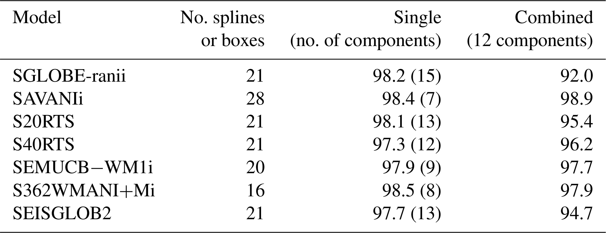
Table 3 Examples of key geophysical patterns recovered in the mantle by the varimax analysis (see Figs. 4 and C1–C6). HV: high-velocity zone, LV: low-velocity zone.

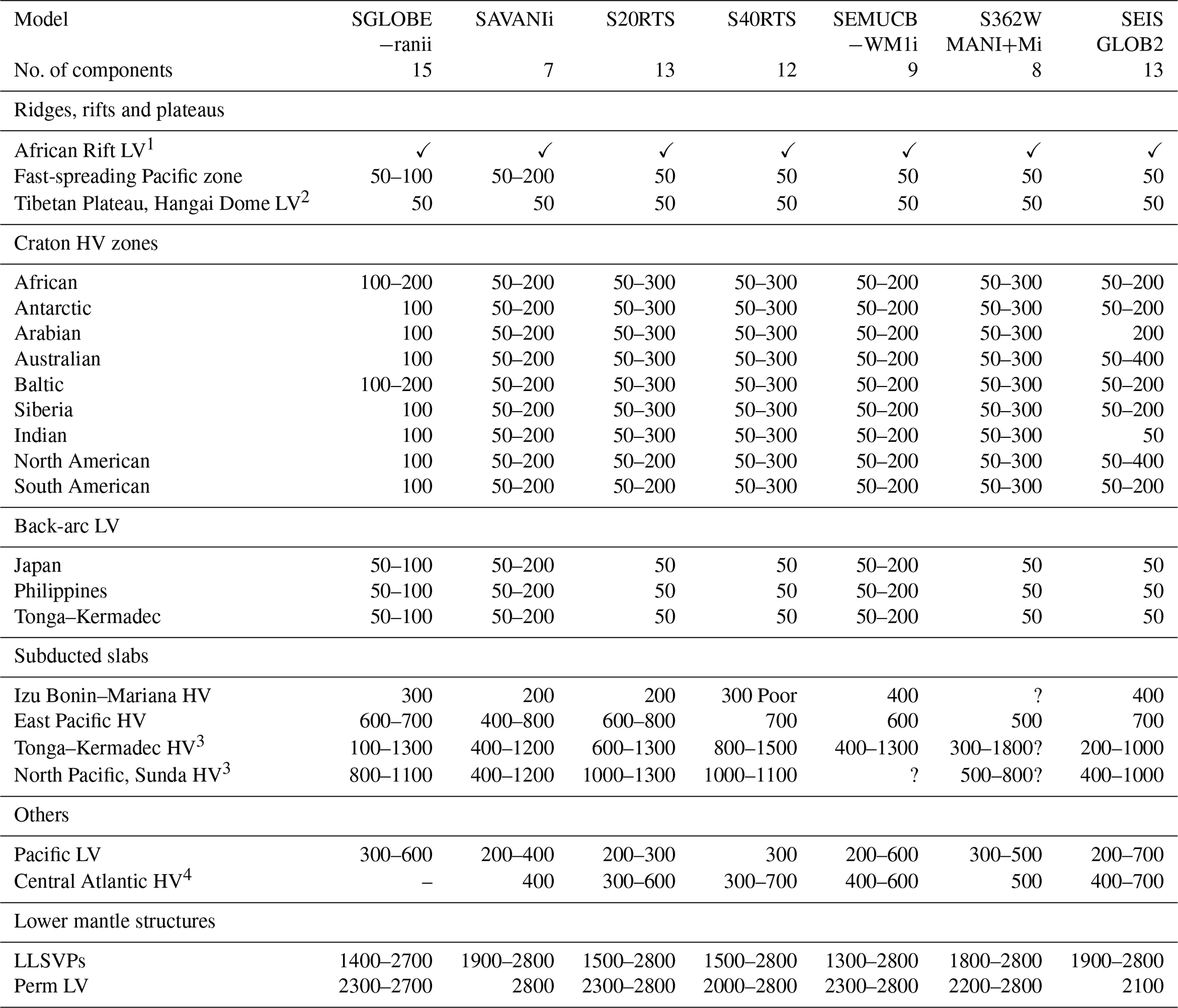
¹ No clear interruption from the surface down to the CMB; ² Legendre et al. (2015), Chen et al. (2015); ³ van der Meer et al. (2018) ⁴ Ritsema et al. (2011).

6 Combined PCA

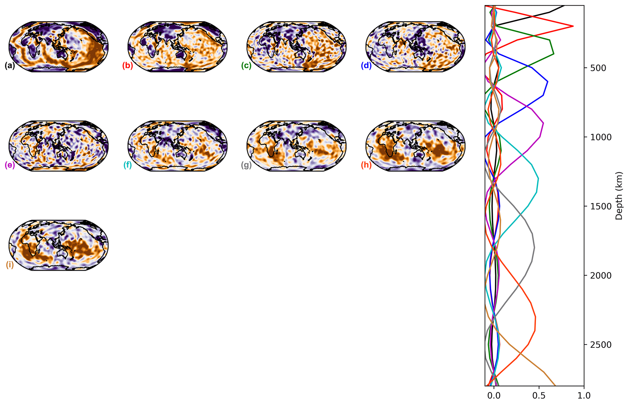
The horizontal patterns associated with each PC result from the projection of the tomography model on the varimax PCs, which differ from one model to the other. As suggested by Sengupta and Boyle (1998) in another context, it is interesting to compare the different models using a common PCA, which removes the inconsistencies between the representations. Thus, we apply a varimax PC analysis to the seven models stacked on the horizontal axis, i.e. to a $\mathrm{7}\times \mathrm{9002}=\mathrm{63014}$ by 29 matrix, and refer to the results as a combined analysis in the remainder of this paper. Using the same 1 % threshold limit as used before, this analysis generates 12 varimax PCs, i.e. 12 vertical profiles (A–L) common to the seven models. Then, we compute the horizontal structures associated with each PC by projecting each of the seven models on those vertical profiles (Figs. 5 and D1–D11).

Figure 5 PC F (maximum at 1000 km of depth) of the combined analysis of the isotropic models. On the right are the principal components or vertical profiles, and on the left are the associated horizontal structures. The other components are shown in the Appendix in Figs. D1–D11.

Components A–D (at ∼ 50, 200, 300 and 600 km depths) are mostly confined in the upper mantle, while lower mantle structure is represented by components E–L (∼ 800, 1000, 1200, 1400, 1700, 2000, 2300 and 2800 km depths), as shown in the vertical profiles from the combined varimax analysis presented in the last column of Fig. 3. As expected, the vertical profiles from the combined analysis are smoother than those from the individual model analysis for the more detailed models (SGLOBE-ranii, SEMUCB−WM1i, S40RTS and SEISGLOB2), and sharper for the smoothest tomography models (SAVANIi, S20RTS, SEMUCB−WM1i and S362WMANI+Mi). Note that the 1 % criterion is applied globally and not to the individual models, as was done in the previous section. The last column of Table 2 shows the total variance captured by the 12 components for each model. It shows that the combined analysis is very efficient for the smooth SAVANIi model, capturing 98.9 % of its variance, whereas the variance captured for the other models lies between 92.0 % and 97.9 %. The SGLOBE-ranii model is only resolved at the 92.0 % level, which is not surprising as it is more detailed than the other models (likely due to the use of less regularisation), with the individual analysis requiring 15 PCs and allowing a finer localisation of the models' patterns (Fig. C1).

Most of the patterns described in Table 3 and discussed in the previous section are also recovered by the combined analysis. This common projection makes it easier to compare the components E (∼ 800 km of depth) to G (∼ 1200 km of depth) in the lower mantle. These components (Figs. 5 and D5–D6) capture ∼ 20.1 % of the information in the models and display a similar pattern in SGLOBE-ranii, S20RTS, S40RTS and SAVANIi. On the other hand, SEMUCB−WM1i, S362WMANI+Mi and SEISGLOB2 show different features, such as e.g. fewer high-velocity zones in this depth range. Regarding principal component H (∼ 1400 km of depth; Fig. D7), it describes 7.2 % of the information. All the models show a similar large-scale pattern except for S362WMANI+Mi, which shows isolated low-velocity zones in the Pacific, especially in the south.

As shown in the previous section, all models display several independent components in the lower mantle, making between 36 % (SAVANIi) and 69 % (SEISGLOB2) of the total components, depending on the model. This highlights complexity in the lower mantle and supports recent studies suggesting that the region of the lower mantle above the lowermost D^′′ layer is more complex than previously thought. For example, slab stagnation and lateral deflection of mantle plumes have been proposed in the uppermost lower mantle (Fukao and Obayashi, 2013; French and Romanowicz, 2015). Moreover, intriguing observations of seismic discontinuities (Kawakatsu and Niu, 1994; Jenkins et al., 2017) and scatterers (Kaneshima, 2016) have also been reported at these depths. Compositional layering (Ballmer et al., 2015), a viscosity increase (Marquardt and Miyagi, 2015; Rudolph et al., 2015) and spin transitions that seem to occur in Fe-bearing mantle minerals (Lin et al., 2013) have been proposed in the lower mantle, which can potentially influence the region's elasticity and transport properties.

6.1 Anisotropic structure

In addition to isotropic shear-wave-speed anomalies, four of the models considered in our study also include radial anisotropy perturbations: that is, speed differences between vertically and horizontally polarised shear waves in SGLOBE-rania, SEMUCB−WM1a, SAVANIa and S362WMANI+Ma. The seismic imaging of anisotropy is more challenging than that of isotropic structure because the sensitivity of seismic data to anisotropy is weaker (e.g. Chang et al., 2014; Beghein and Trampert, 2004; Romanowicz and Wenk, 2017). Moreover, it has been shown that if crustal effects are not properly modelled, this can lead to substantial errors in the estimated mantle anisotropy (Panning et al., 2010; Ferreira et al., 2010; Chang et al., 2016; Bozdağ and Trampert, 2008; Lekić et al., 2010). These difficulties are at least partly responsible for the strong differences between existing radial anisotropy models (e.g. Fig. A1b). Varimax PC analysis is thus a natural candidate to analyse and compare the models since it enhances their robust information. Figures E3 and E1–E10 show the vertical profiles (varimax PCs) and horizontal patterns from the combined varimax analysis on the anisotropic part of the four radially anisotropic models, for which 10 components capture more than 1 % of the variance. As expected, there is poorer agreement between the radial anisotropy structure in the models than between the isotropic structure discussed in the previous sections, though some common features can be identified.

The two LLSVPs appear on the deepest PC J of SGLOBE-rania and SEMUCB−WM1a (Fig. E10), which captures 10 % of the models' information. The Pacific LLSVP barely appears in the last PC for SAVANIa and S362WMANI+Ma. However, as explained in Sect. 3, e.g. Kustowski et al. (2008), Chang et al. (2014), and Chang et al. (2015) showed that the signature of LLSVPs in radial anisotropy models is an artefact due to leakage of isotropic structure into artificial anisotropic structure in the lowermost mantle.

For PC B (with a maximum at ∼ 100 km of depth; Fig. E2), a positive zone appears beneath the Pacific and the Nazca plates in SGLOBE-rania, SAVANIa and to a lesser extent SEMUCB−WM1a, while no clear pattern is evidenced in S362WMANI+Ma. The same holds true for mid-ocean ridges. A positive anomaly is observed on PC C under the Pacific Plate for all models, with a maximum around a depth of 200 km (Fig. E3). A broad positive radial anisotropy anomaly beneath the Pacific at these upper mantle depths has been well-documented in previous studies and may be due to horizontal mantle flow in the region and/or thin layers of partial melt in the asthenosphere (e.g. Ekström and Dziewonski, 1998; Gung et al., 2003).

Components B (maximum depth 100 km; Fig. E2), D (maximum depth 400 km; Fig. E4) and especially C (Fig. E3) evidence subduction patterns in SGLOBE-rania (Alaska, Izu–Bonin, Fiji–Tonga–Kermadec). This is also observed, but less clearly, for SAVANIa and S362WMANI+Ma on PC C. We also distinguish subduction signatures deeper in the mantle on PC F along Cascadia, Central and South America, Tonga, the western Pacific, and the north of the Mediterranean Sea (Fig. E6). An overall red negative anisotropy anomaly for the first (PC A) is common to SEMUCB−WM1a and SAVANIa (Fig. E1). SGLOBE-rani shows such a red anomaly only under the oceans, which is probably due to the different way the crust is treated in this model, with crustal thickness perturbations being jointly inverted along with isotropic and anisotropic structure (Chang et al., 2015).

7 Conclusions

Global seismic tomography models typically involve thousands to tens of thousands of parameters, which can be cumbersome to handle and difficult to interpret. This is also true for model comparison; we lack a common basis for comparing models built with different parameterisations. In this study we used a rotated version of principal component analysis to compress the information and ease the geological interpretation and model comparison. The varimax PC analysis results in a separation of the information into different components associated with depth distributions, which are linked to a horizontal pattern obtained by orthogonal projection. We tested the analysis on seven global tomography models: S20RTS, S40RTS, SEISGLOB2, SEMUCB−WM1, SAVANI, SGLOBE−rani and S362WMANI+M; the latter four include laterally varying radial anisotropy. We analysed the models both individually and jointly.

We found that by using the varimax method we reduced the number of independent depth components needed to describe more than 97 % of the total information in the tomography models by 29 % to 75 %. We note that the scale of heterogeneity is not relevant for the varimax PCA method, which is only based on the vertical covariance. Considering the low amount of variance lost in the reconstruction (e.g. Fig. 4) and the spectrum shown in the Appendix, we capture most of the information, and we do not change the spectrum of the signal. Thus, the method is valid for any scale, as long as the signal is robust. In the varimax comparison, what is called noise is not the small-scale features, but rather the part of the models that is not covariant vertically. Hence, the varimax analysis simplifies the number of patterns that needs to be analysed without any significant loss of information; by ensuring the orthogonality of the depth components, it eased the detection and comparison of the relevant information. Overall, the large majority of depth components and horizontal maps obtained from the varimax analysis are different from the original parameterisations used for building the models. This is especially true above the 600 km discontinuity and in the whole mantle for the SAVANIi, S362WMANI+Mi and SEMUCB−WM1i models, wherein the information is recovered by fewer PCs than the spline functions. This implies that the PCs do not only reflect the model parameterisation and inform us about the independence between the slices reconstructed from the model. This also shows that the tomography models do not have a strong imprint of their model parameterisation. The varimax technique, being a data compression method, allows an easier view of all information present in the tomography models and is complementary to clustering methods, such as the k-means technique, which allow us to evidence zones of comparable properties. Both can help users get a better understanding of the Earth's complex interior structure.

Being data-based, the varimax method is neutral with respect to the assumptions made in the model's construction. The combined multi-model varimax analysis allows the comparison of the various tomography models on a neutral set of modes determined by the level of compression fixed by the user. Based on the vertical consistency between the various tomography models, it provides a set of data-based vertical distribution functions. Those functions represent the information present in the PC-based reconstruction and how the models relate to each other. It is fast and simple to implement, and, as we maximise the captured variance, the level of compression is lower for a given number of components and depths than would be required by other methods such as k-means. As the truncation level is a free parameter, the user controls the amount of signal suppressed from the compression to an arbitrary level.

When applying the varimax analysis to isotropic tomography models, we found that the most important elements of the models contributing to most of the information are (i) large low-shear-velocity provinces (LLSVPs) in the lowermost mantle, (ii) subducted slabs and low-velocity anomalies probably associated with mantle plumes in the upper and lower mantle, and (iii) ridges and cratons in the uppermost upper mantle. The analysis highlights several independent components in the lower mantle that make between 36 % and 69 % of the total components depending on the model, which supports recent studies suggesting that the lower mantle is more complex than previously thought. The reasons for this complexity remain a very active field of research. On the other hand, we find limited agreement between the radial anisotropy structure of the models, with common features mainly in the asthenosphere and to some extent in the lower mantle beneath the Pacific and beneath subduction zones.

Choices such as data types and amounts, as well as the strength of regularisation used in the construction of tomography models are probably key controls on the number of varimax components required by each model. Hence, the PCA-based model compression preserves the impact of the choices made in the construction of the tomography models and facilitates their interpretation in terms of geophysical objects. Future work will expand this analysis for the interpretation and comparison of local and regional models, which tend to use more diverse underlying datasets than in global models and have highly variable spatial resolutions. Moreover, we will also focus on comparisons with other sources of information, such as geodynamical models, gravity anomalies, magnetic anomalies and heat fluxes.

Appendix A: Models

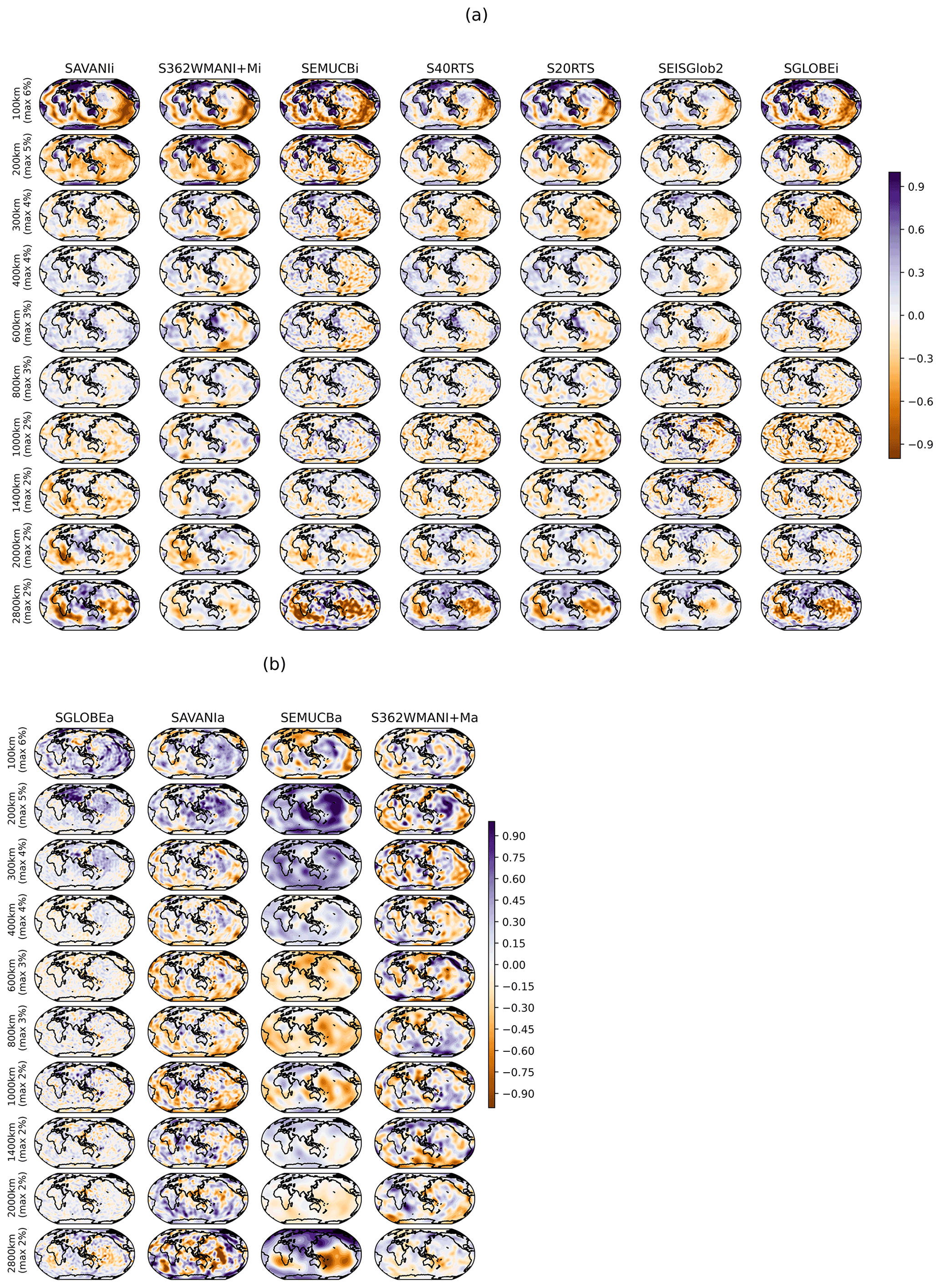
Figure A1 Depth slices of the isotropic and anisotropic models used in this study at the depths of 100, 200, 300, 400, 600, 800, 1000, 1400, 2000 and 2900 km. The isotropic (a) and anisotropic (b) models show perturbations in shear-wave speed and in $\mathit{\xi }=V_{\mathrm{SH}}^{\mathrm{2}}/V_{\mathrm{SV}}^{\mathrm{2}}$ with respect to PREM (Dziewonski and Anderson, 1981), respectively. The colour scale is normalised to vary from −max to +max, with the range of model amplitude variations shown at the left of each row. For simplicity, in the remainder of this paper we add the letter “i” to the tomography models' names when referring to their isotropic part and we add the letter “a” when referring to their radially anisotropic part; in the different figures “SGLOBE” will stand for SGLOBE-rani and “SEMUCB” for SEMUCB-WM1.

Appendix B: Comparison of the original and the reconstructed models

B1 Spatial domain

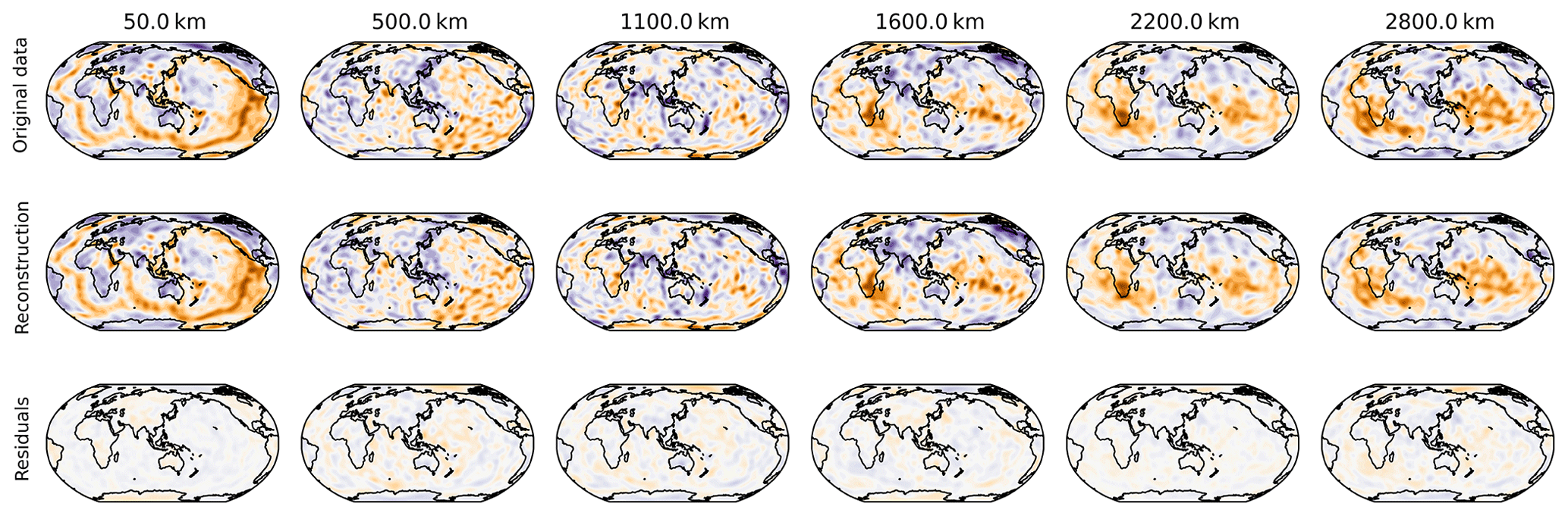
Figure B1 Examples of six depth slices in the original SEMUCB−WM1i model (top), in the model recovered without the principal components with less than 1 % of the variance, i.e. with nine components (middle), and differences between the two (bottom).

B2 Spectral domain

Figure B2 PSDs of the original models.

Figure B3 PSDs of the reconstructed models from the varimax modes. The number of modes is given in Table 2.

Appendix C: Varimax PCA of isotropic models

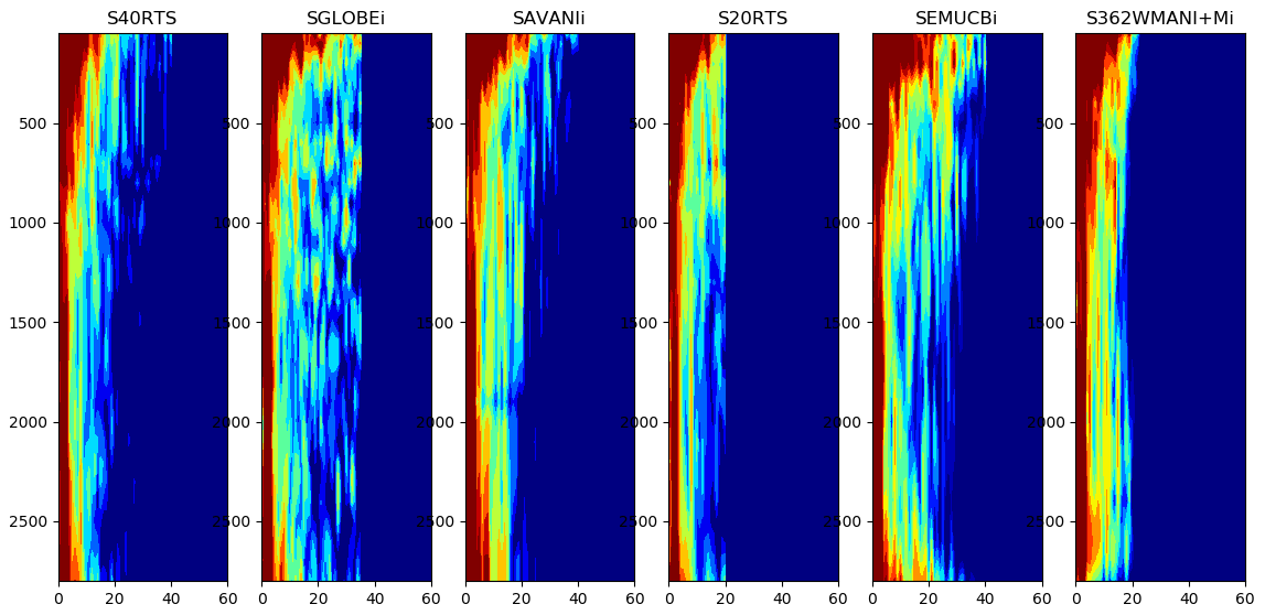
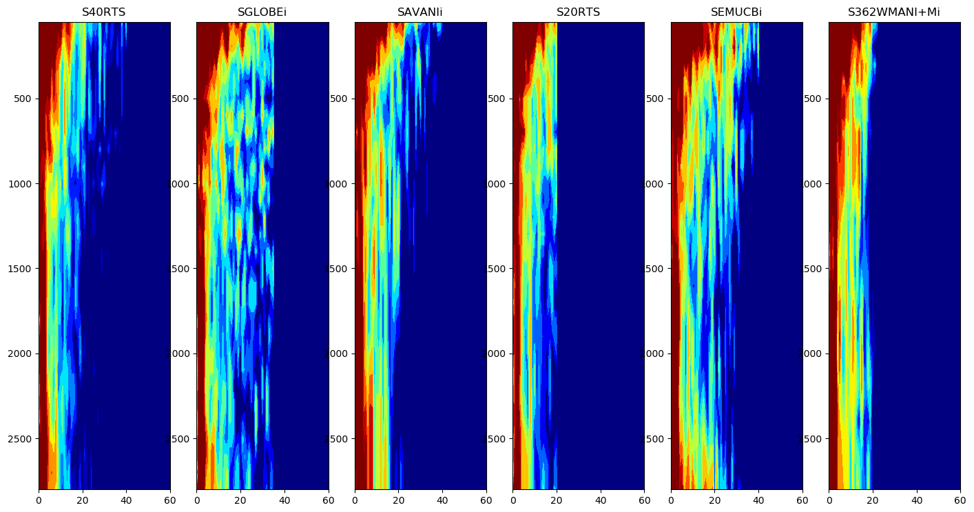
Figure C1 The 15 varimax components of the isotropic part of the SGLOBE-rani model. On the right are the principal components or vertical profiles, and on the left are the associated horizontal structures.

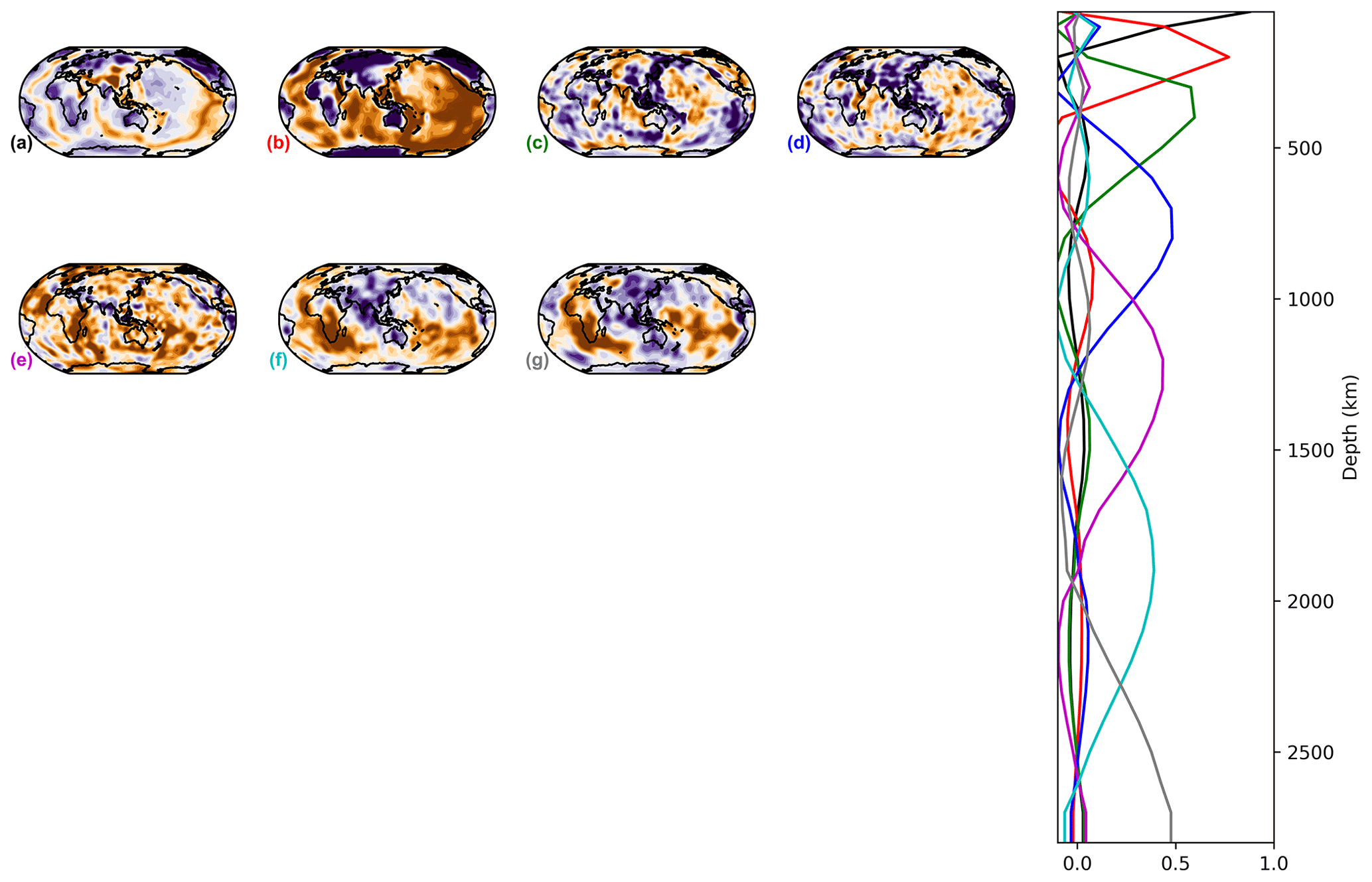
Figure C2 The seven varimax components of the isotropic part of the SAVANI model.

Figure C3 The 13 varimax components of the S20RTS model.

Figure C4 The 12 varimax components of the S40RTS model.

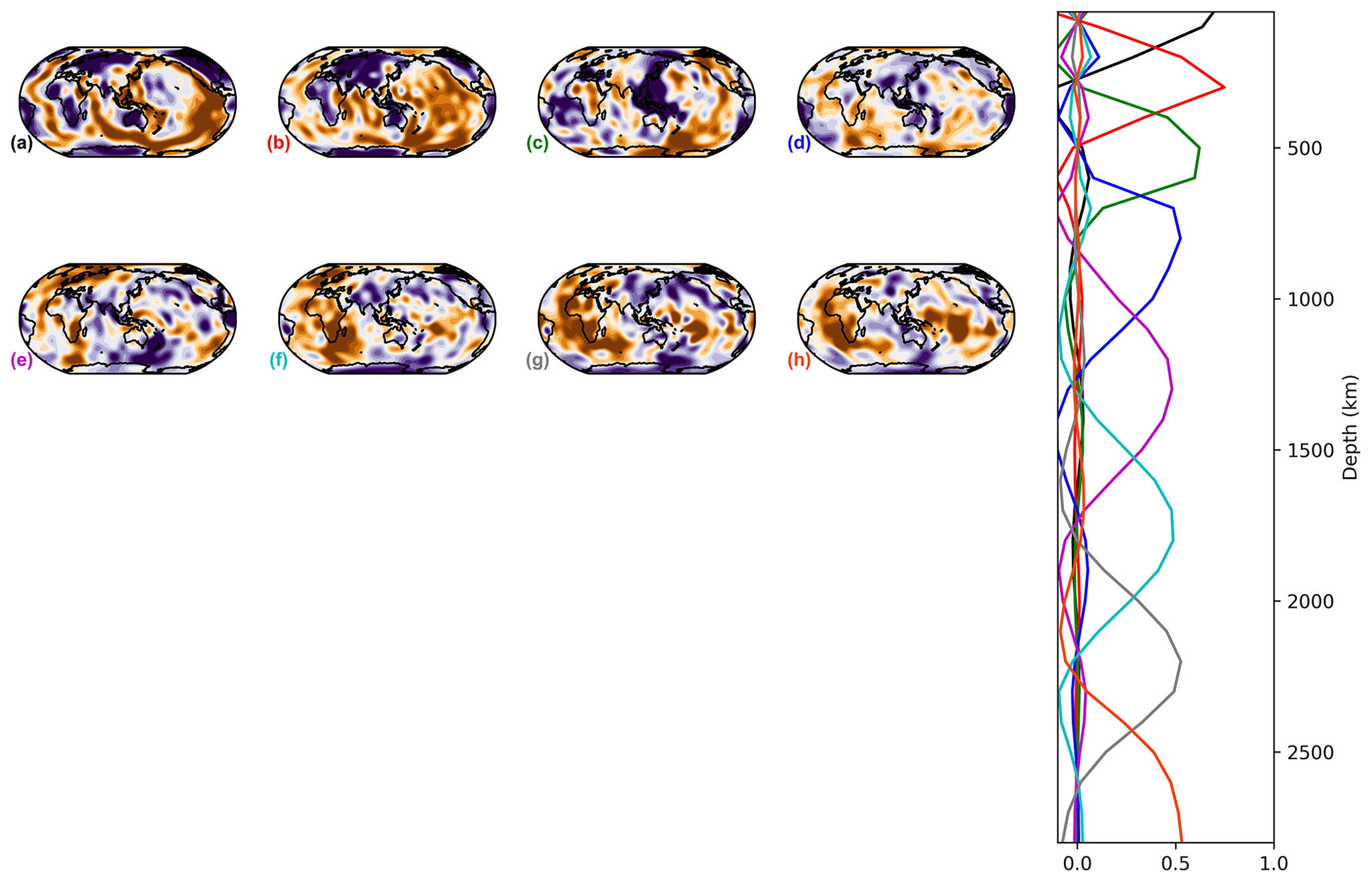
Figure C5 The eight varimax components of the isotropic part of the S362WMANI+M model.

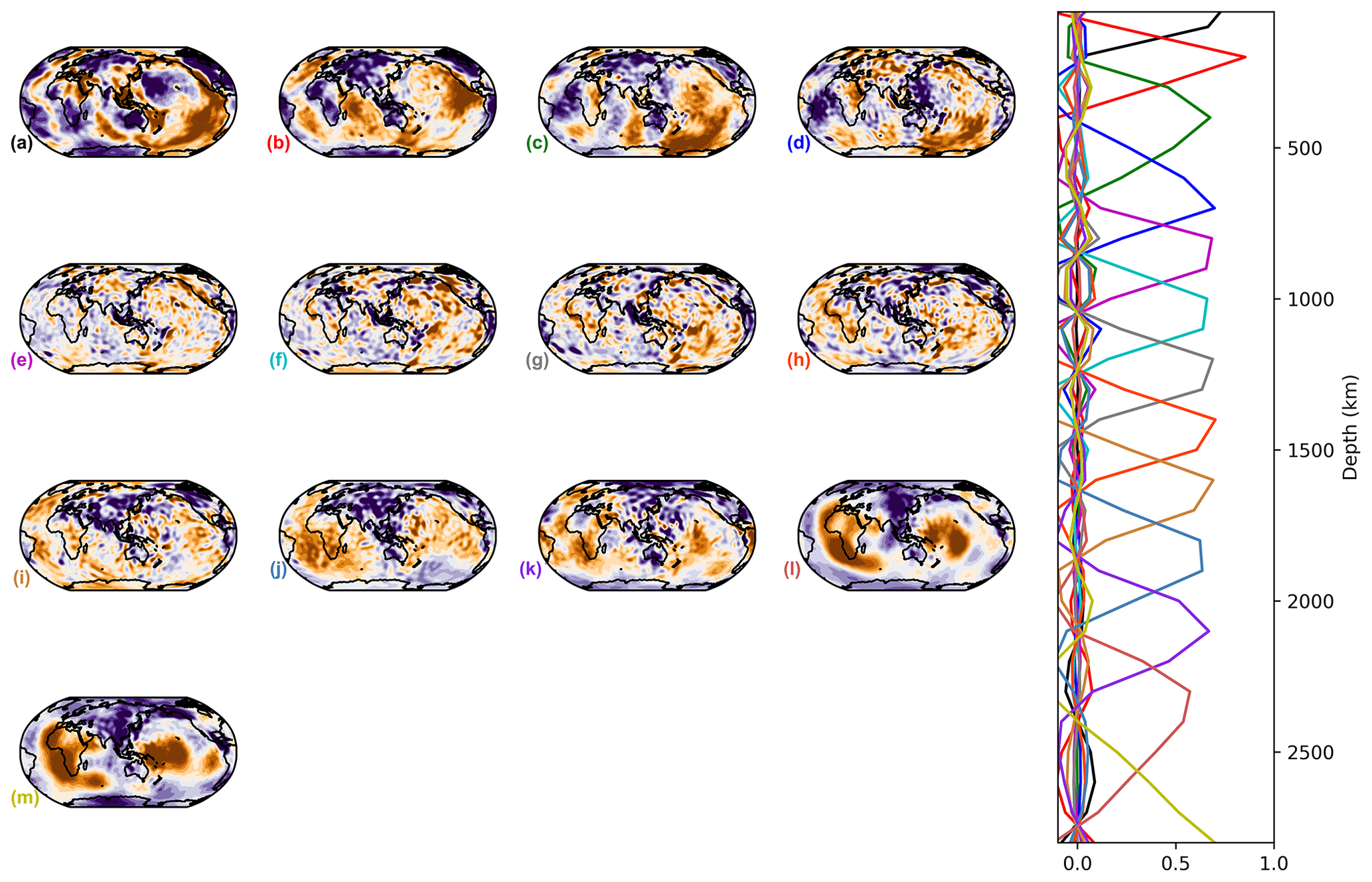
Figure C6 The 13 varimax components of the isotropic part of the SEISGlob2 model.

Appendix D: Combined PCA of isotropic models

Figure D1 PC A (maximum at 50 km of depth) of the combined analysis of the isotropic parts of the models. On the right are the principal components or vertical profiles, and on the left are the associated horizontal structures.

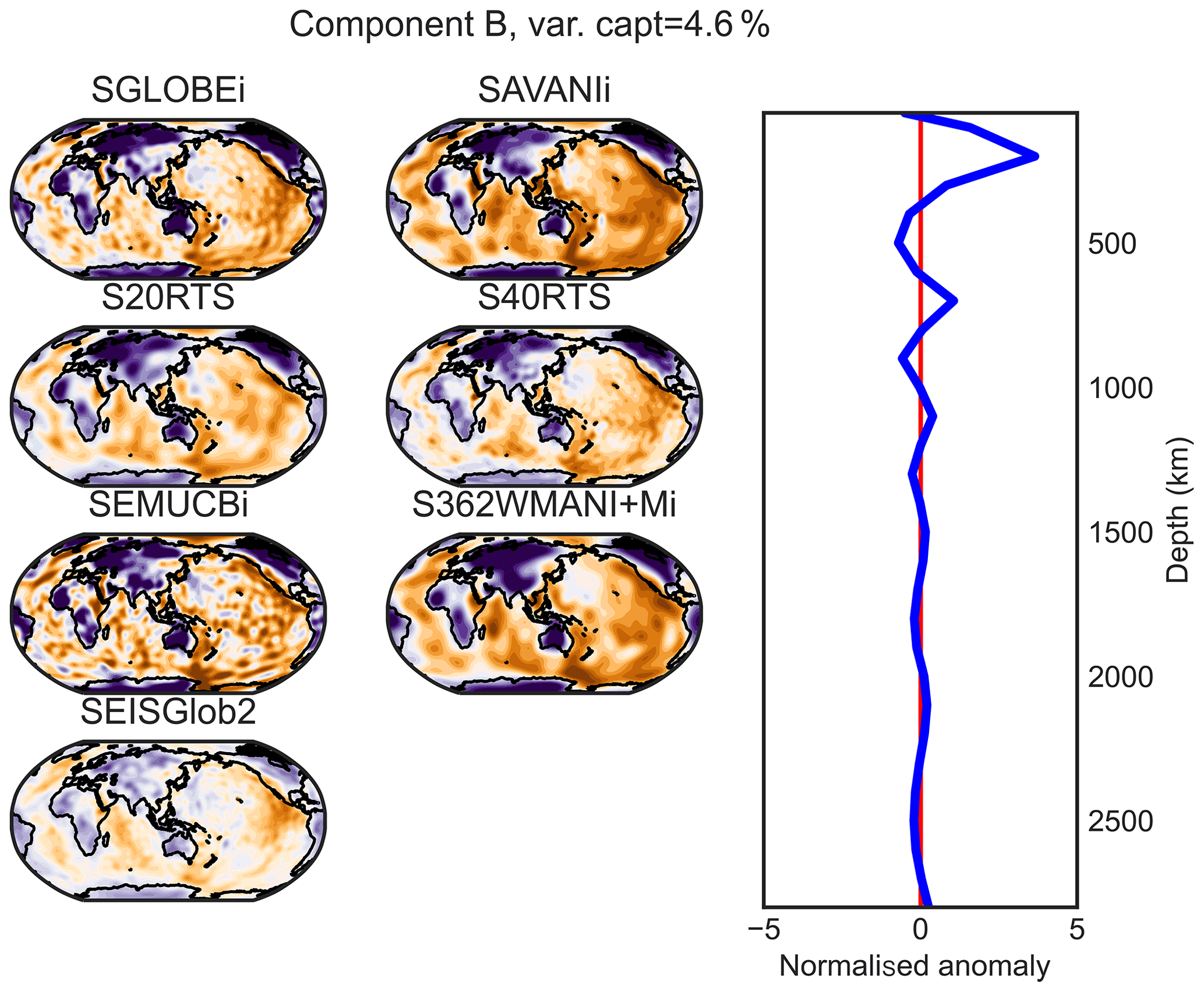
Figure D2 PC B (maximum at 200 km of depth) of the combined analysis of the isotropic parts of the models.

Figure D3 PC C (maximum at 300 km of depth) of the combined analysis of the isotropic parts of the models.

Figure D4 PC D (maximum at 600 km of depth) of the combined analysis of the isotropic parts of the models.

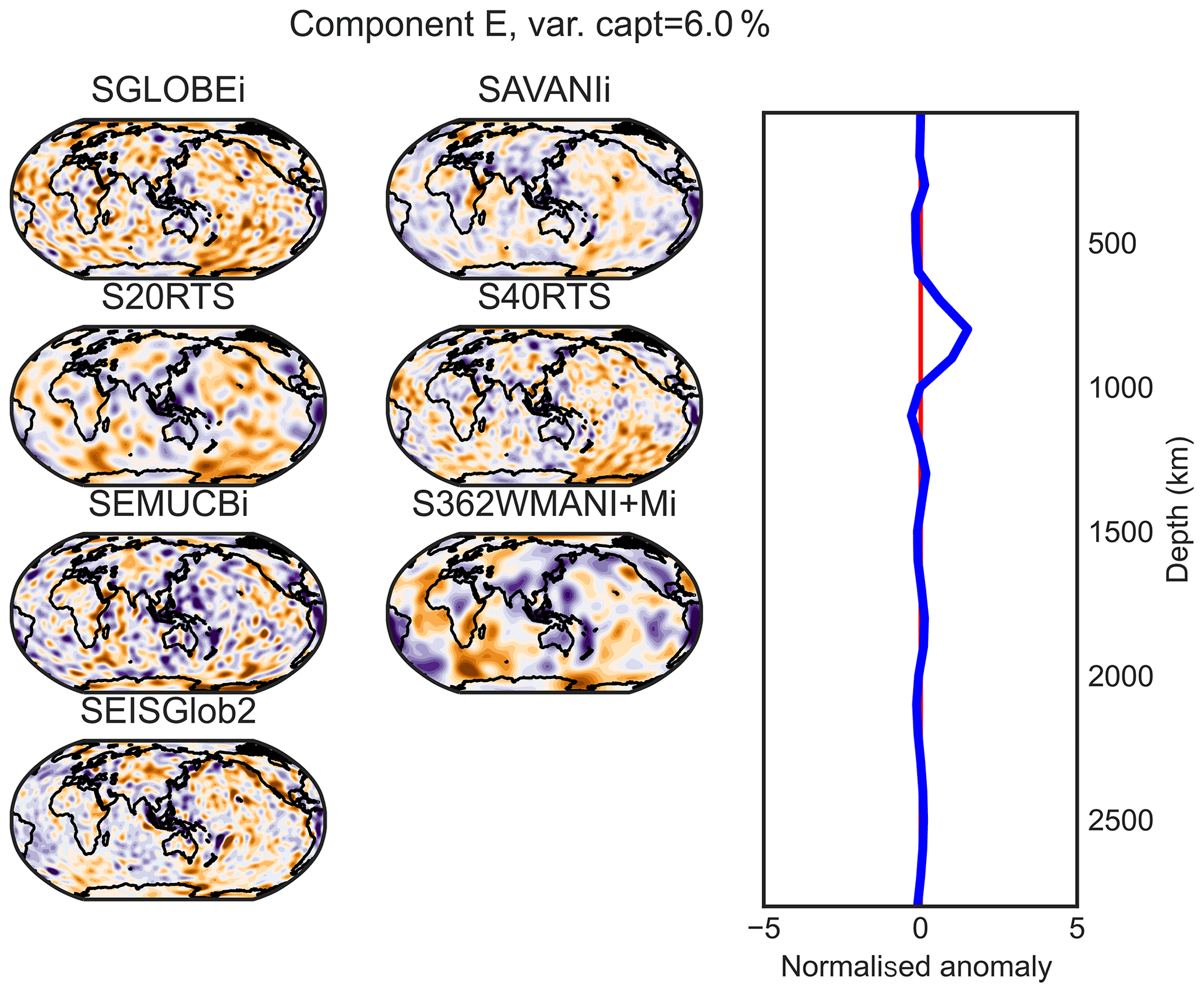
Figure D5 PC E (maximum at 800 km of depth) of the combined analysis of the isotropic parts of the models.

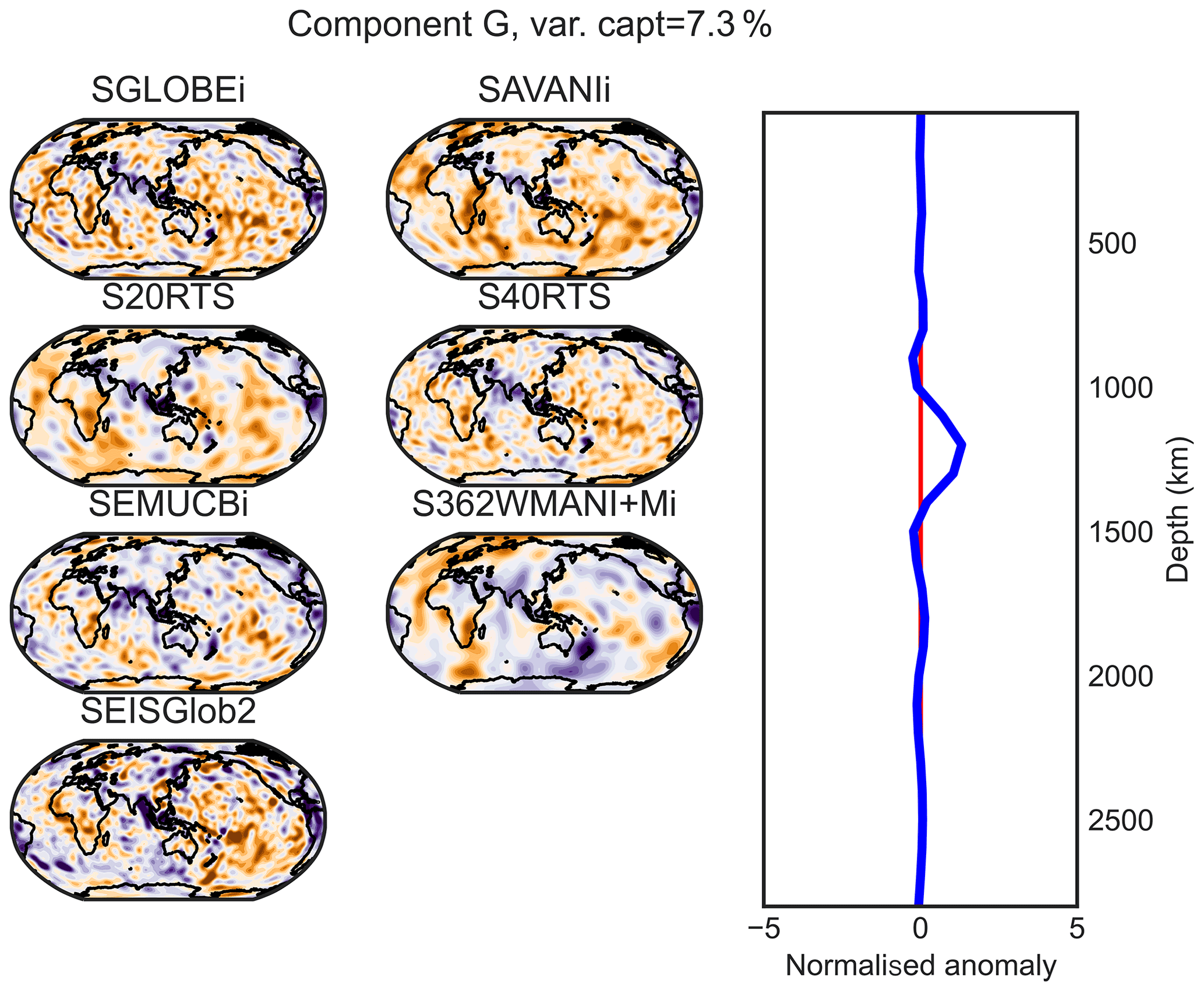
Figure D6 PC G (maximum at 1200 km of depth) of the combined analysis of the isotropic parts of the models.

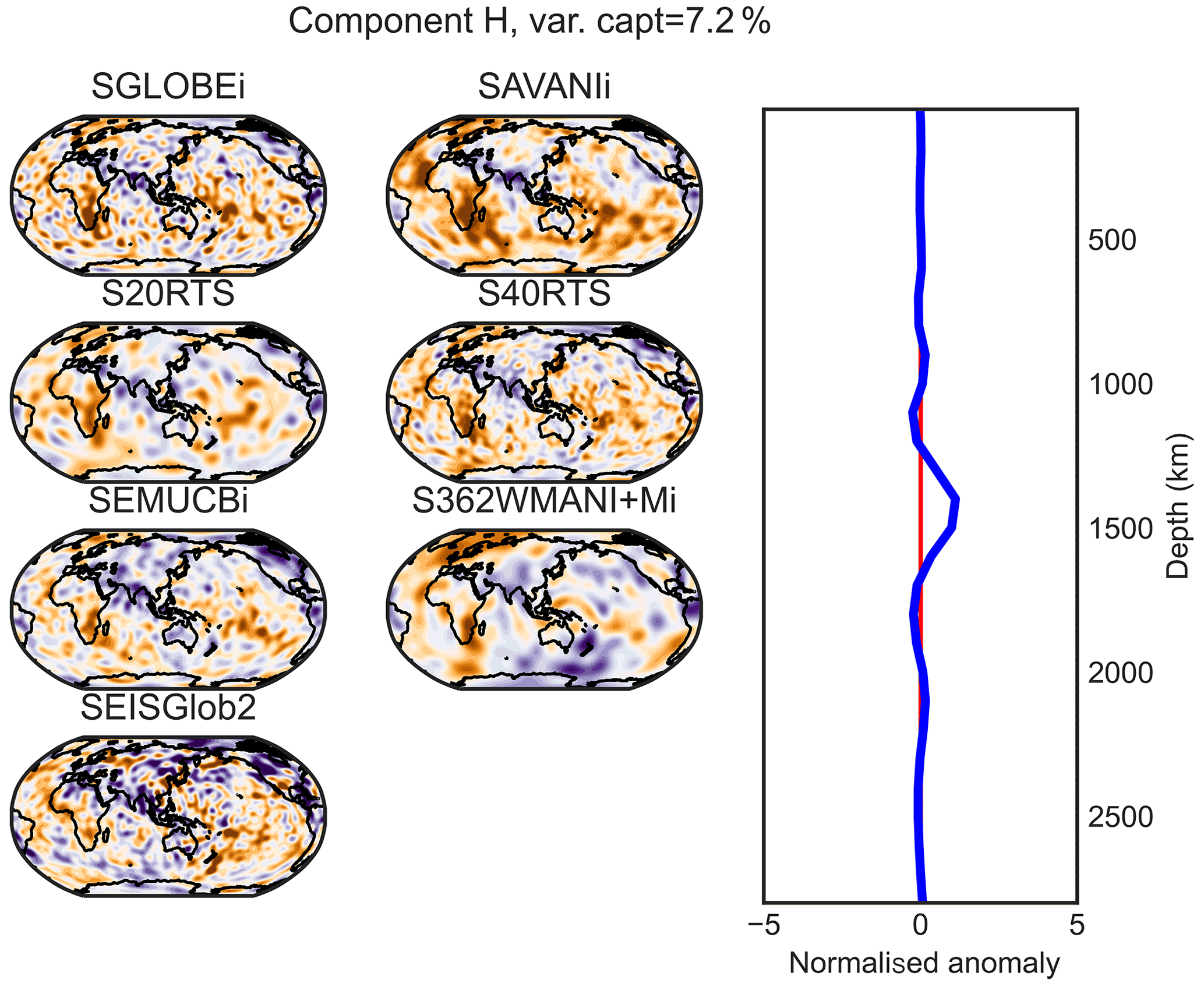
Figure D7 PC H (maximum at 1400 km of depth) of the combined analysis of the isotropic parts of the models.

Figure D8 PC I (maximum at 1700 km of depth) of the combined analysis of the isotropic parts of the models.

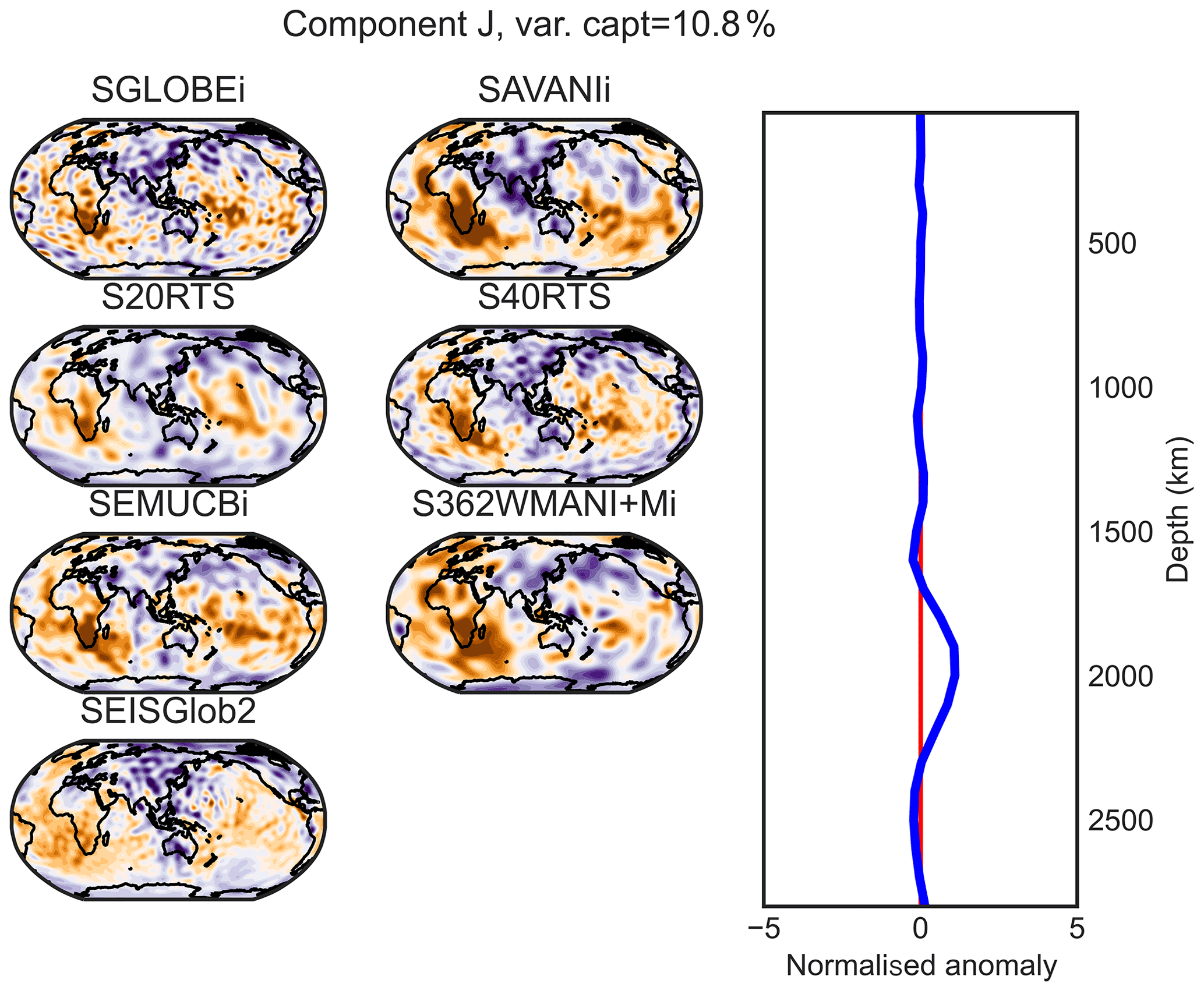
Figure D9 PC J (maximum at 2000 km of depth) of the combined analysis of the isotropic parts of the models.

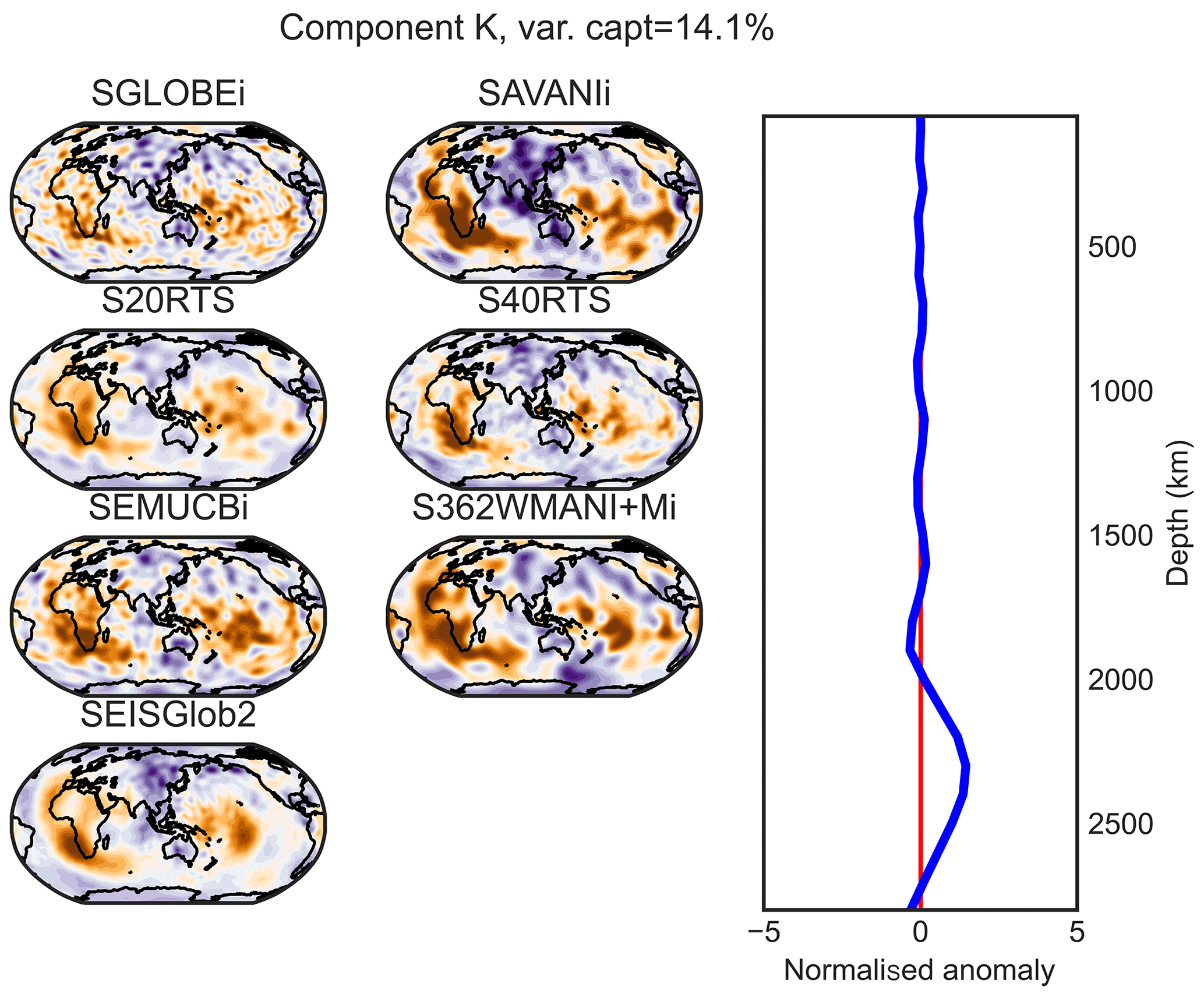
Figure D10 PC K (maximum at 2300 km of depth) of the combined analysis of the isotropic parts of the models.

Figure D11 PC L (maximum at 2800 km of depth) of the combined analysis of the isotropic parts of the models.

Appendix E: Combined PCA of anisotropic models

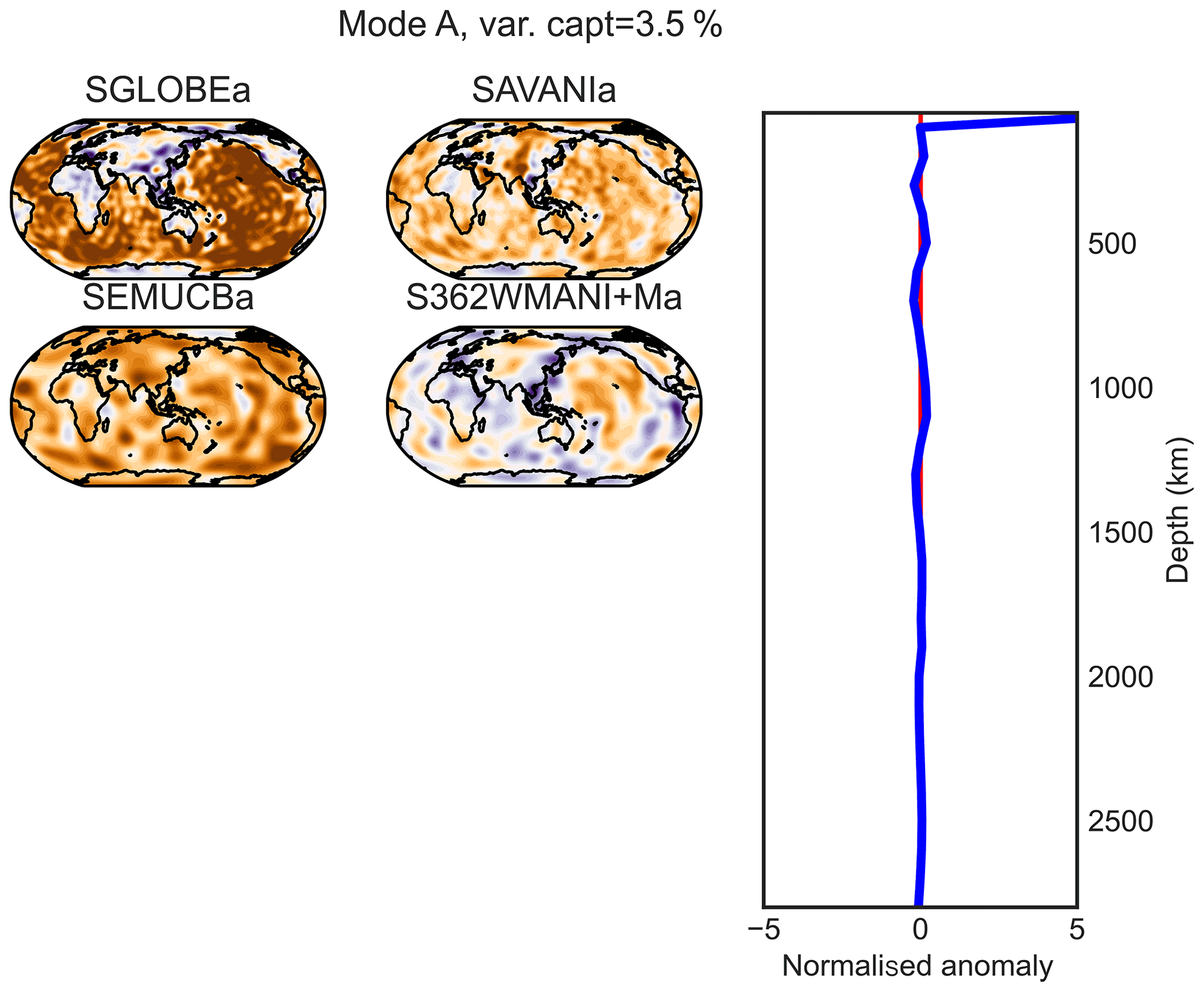
Figure E1 PC A (maximum at 50 km of depth) of the combined analysis of the anisotropic parts of the models. On the right are the principal components or vertical profiles, and on the left are the associated horizontal structures.

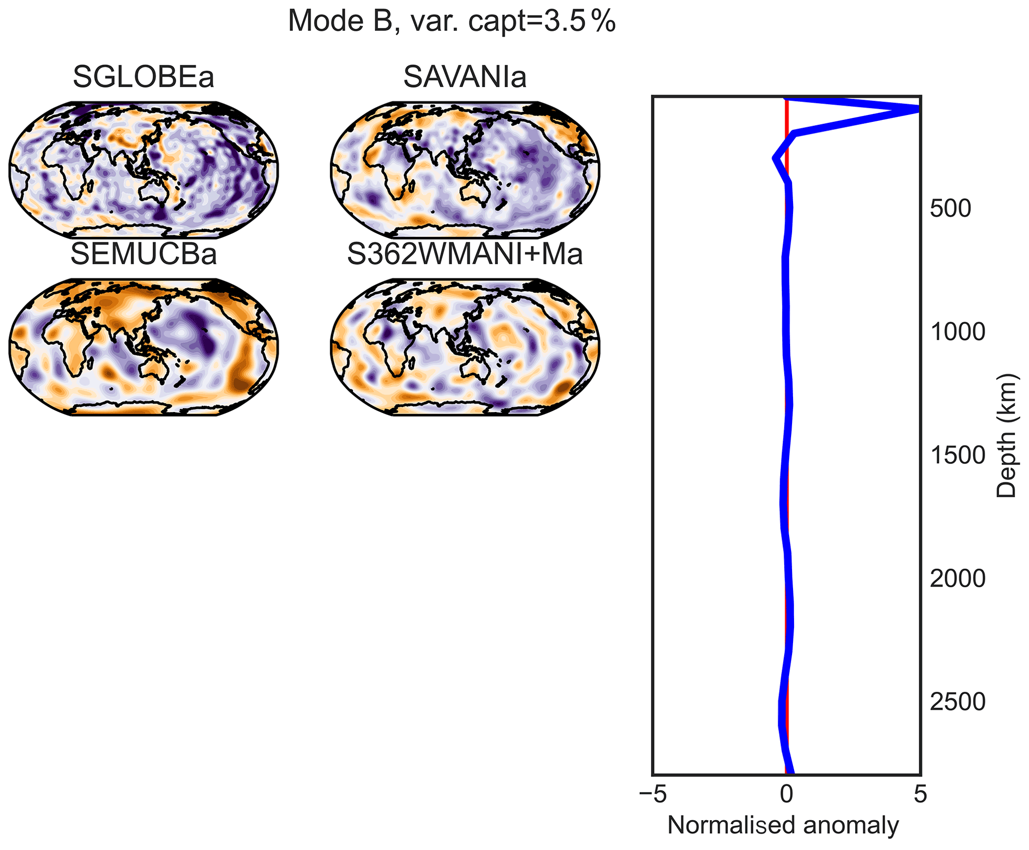
Figure E2 PC B (maximum at 100 km of depth) of the combined analysis of the anisotropic parts of the models.

Figure E3 PC C (maximum at 200 km of depth) of the combined analysis of the anisotropic models.

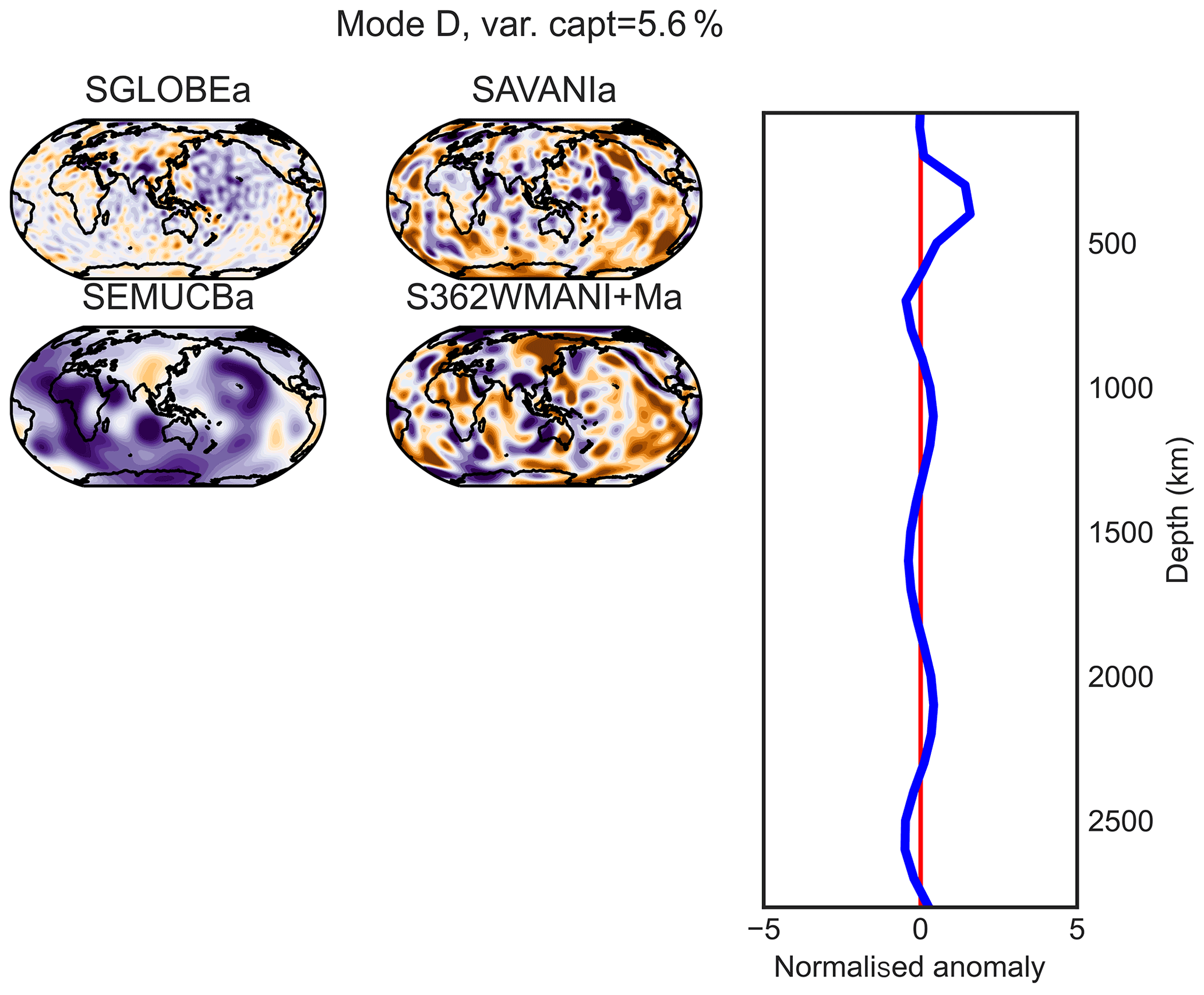
Figure E4 PC D (maximum at 400 km of depth) of the combined analysis of the anisotropic parts of the models.

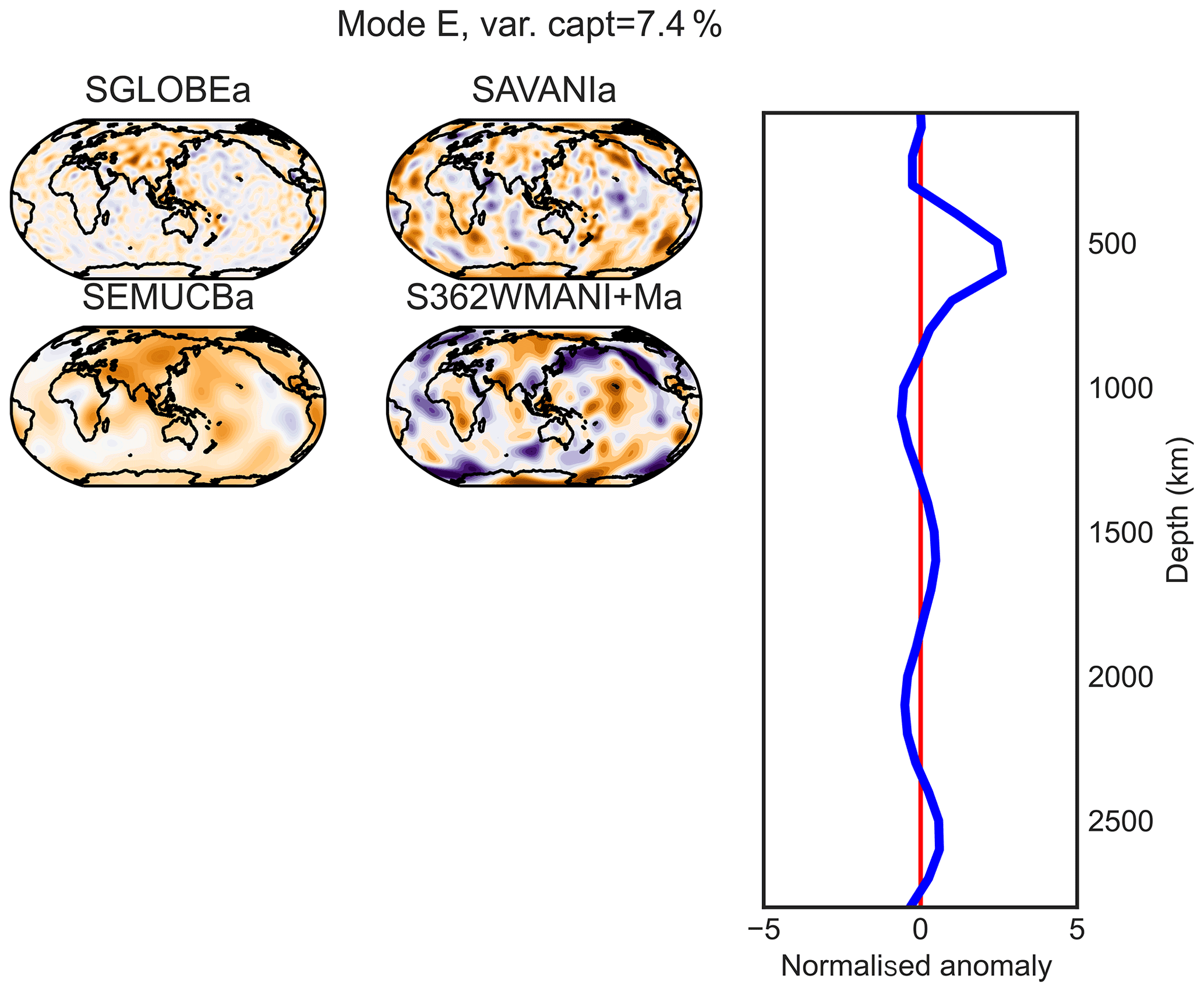
Figure E5 PC E (maximum at 600 km of depth) of the combined analysis of the anisotropic parts of the models.

Figure E6 PC F (maximum at 800 km of depth) of the combined analysis of the anisotropic parts of the models.

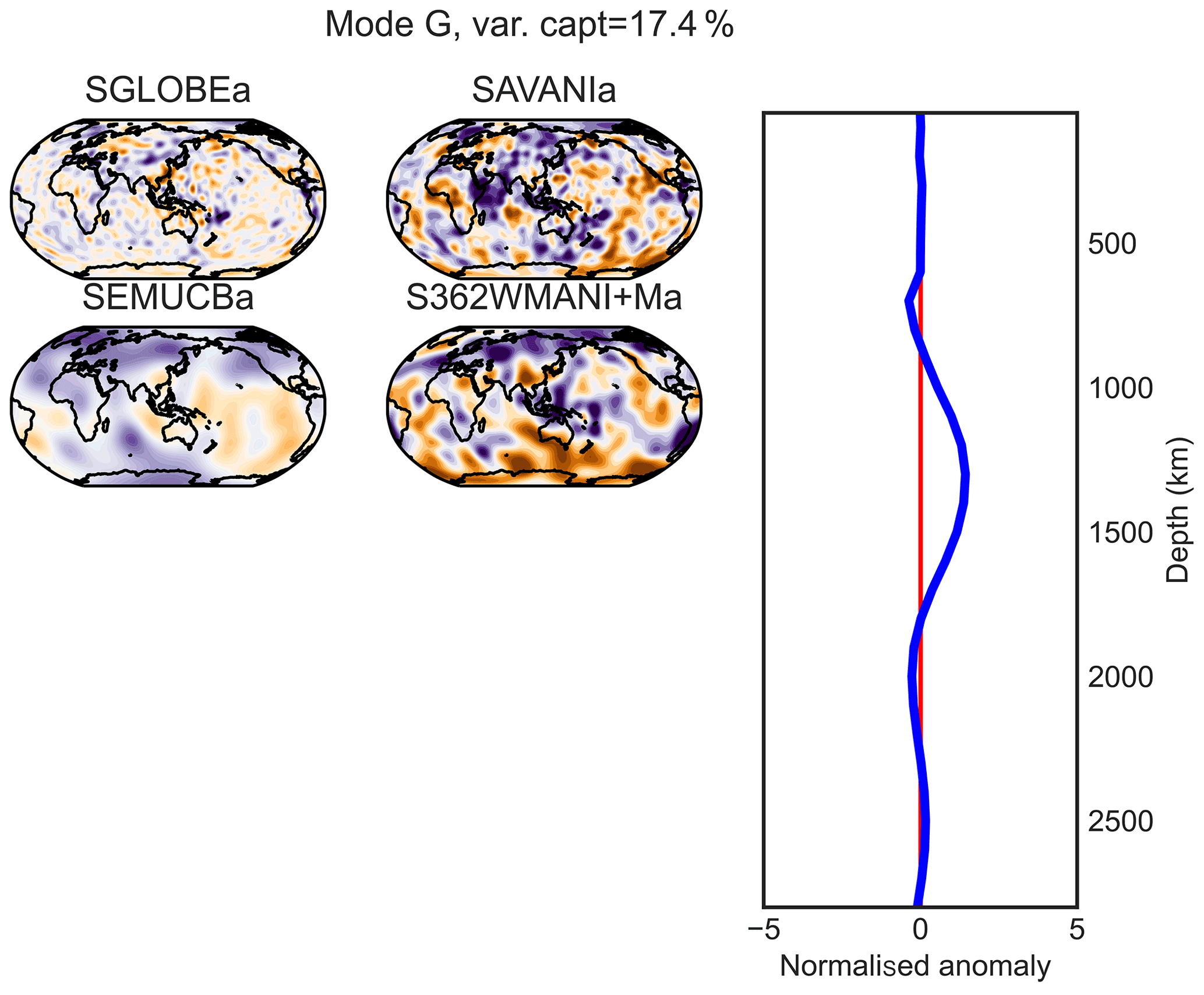
Figure E7 PC G (maximum at 1300 km of depth) of the combined analysis of the anisotropic parts of the models.

Figure E8 PC H (maximum at 1900 km of depth) of the combined analysis of the anisotropic parts of the models.

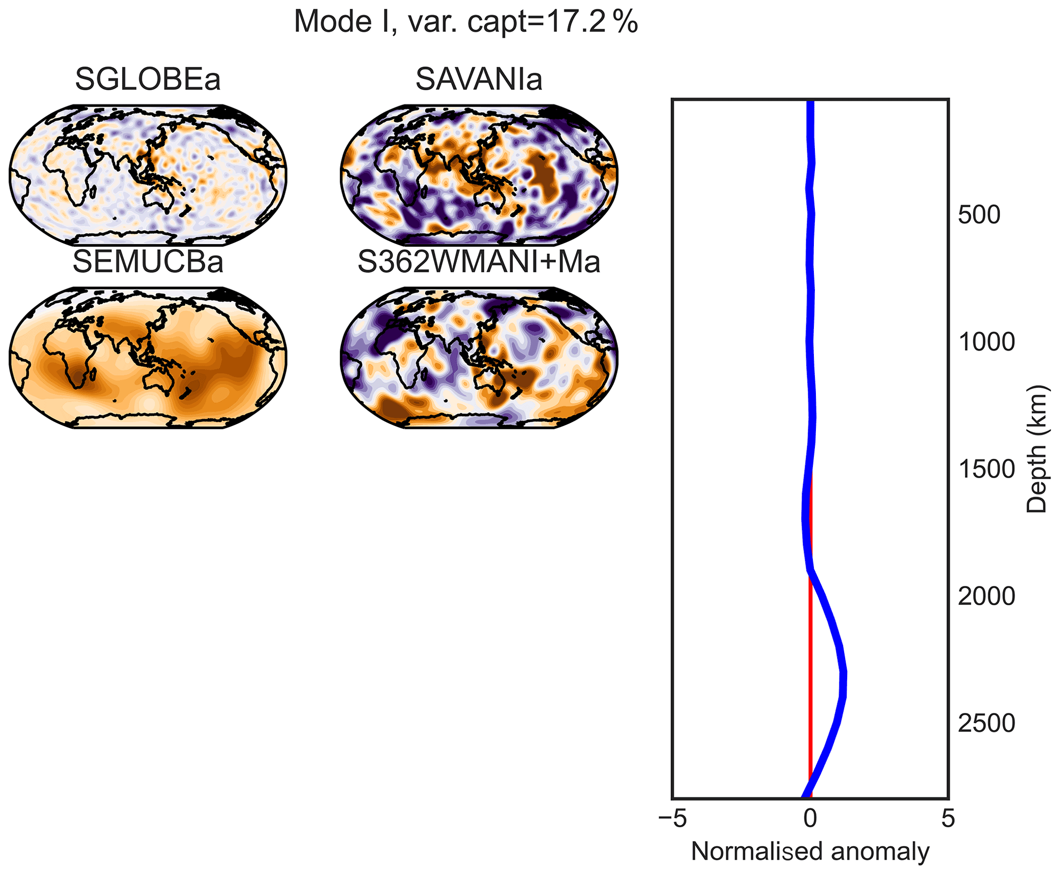
Figure E9 PC I (maximum at 2300 km of depth) of the combined analysis of the anisotropic parts of the models.

Figure E10 PC J (maximum at 2800 km of depth) of the combined analysis of the anisotropic parts of the models.