Investigating spatial heterogeneity within fracture networks using hierarchical clustering and graph distance metrics

Rock fractures organize as networks, exhibiting natural variation in their spatial arrangements. Therefore, identifying, quantifying, and comparing variations in spatial arrangements within network geometries are of interest when explicit fracture representations or discrete fracture network models are chosen to capture the influence of fractures on bulk rock behaviour. Treating fracture networks as spatial graphs, we introduce a novel approach to quantify spatial variation. The method combines graph similarity measures with hierarchical clustering and is applied to investigate the spatial variation within large-scale 2-D fracture networks digitized from the well-known Lilstock limestone pavements, Bristol Channel, UK. We consider three large, fractured regions, comprising nearly 300 000 fractures spread over 14 200 m² from the Lilstock pavements. Using a moving-window sampling approach, we first subsample the large networks into subgraphs. Four graph similarity measures – fingerprint distance, D-measure, Network Laplacian spectral descriptor (NetLSD), and portrait divergence – that encapsulate topological relationships and geometry of fracture networks are then used to compute pair-wise subgraph distances serving as input for the statistical hierarchical clustering technique. In the form of hierarchical dendrograms and derived spatial variation maps, the results indicate spatial autocorrelation with localized spatial clusters that gradually vary over distances of tens of metres with visually discernable and quantifiable boundaries. Fractures within the identified clusters exhibit differences in fracture orientations and topology. The comparison of graph similarity-derived clusters with fracture persistence measures indicates an intra-network spatial variation that is not immediately obvious from the ubiquitous fracture intensity and density maps. The proposed method provides a quantitative way to identify spatial variations in fracture networks, guiding stochastic and geostatistical approaches to fracture network modelling.

1 Introduction

Fracture networks in rocks develop due to loading paths that vary over geological timescale (Laubach et al., 2019). The evolution of the network exhibits characteristics of a complex system. There is feedback between the evolving spatial structure and the rock substrate in which the networks are positioned (Laubach et al., 2018). The resulting spatial arrangement that emerges after cumulative network evolution is of considerable interest as it influences flow, transport, and geomechanical stability in multiple anthropogenic subsurface applications such as geothermal energy (Vidal et al., 2017), nuclear waste disposal (Wang and Hudson, 2015), aquifer management (Witherspoon, 1986), and hydrocarbon exploitation (Nelson, 2001). Systematically documenting near-surface fracture patterns is essential, for example, in mining applications where fracture patterns often provide clues to ore deposit patterns (Jelsma et al., 2004), and in geotechnical engineering, where fractures influence stability in human-made structures such as tunnels (Lei et al., 2017).

An important property of natural fracture networks is that of spatial organization, which means that the arrangements are not random but follow a statistically discernable pattern. One can view the spatial arrangement of fractures as a set of objects within a geographical reference system. Within such a framework, fracture objects are either regularly spaced, irregularly spaced with statistically significant regions of close spacing, and irregularly spaced with statistically insignificant regions of close spacing (Laubach et al., 2018). An alternate framework is a network, where fracture objects are described in relation to one another (Valentini et al., 2007; Andresen et al., 2013; Sanderson and Nixon, 2015). Spatial variations in fracture network organization are quite common. The physical phenomena commonly used to explain spatial variation in fracture arrangements are stress shadowing, layer thickness differences, host rock lithology, layered mechanical anisotropy, high-strain events such as faulting/folding, and diagenesis. However, it is generally not easy to associate a type of spatial arrangement to any unique set of input boundary conditions as similar loading paths can lead to diverging patterns, and dissimilar loading paths can lead to converging patterns (Laubach et al., 2019).

Quantifying variations in spatial arrangements of fractures involves the sampling of fracture data. Such quantifications can be in the form of 1-D (using scanline methods, borehole sampling), in 2-D (fracture trace maps from outcrop imagery), or 3-D (ground-penetrating radar, microseismic). 1-D scanlines provide a method to quantify arrangements and variation, and several statistical measures have been proposed, such as fracture spacing (Priest and Hudson, 1976), fracture intensity (Dershowitz and Herda, 1992), coefficient of variation (Gillespie et al., 1993), normalized correlation count (Marrett et al., 2018), and cumulative spacing derivative (Bistacchi et al., 2020). These measurements, however, only indicate the variation of fracture arrangements on the scanline and fail to depict the variation in directions away from the scanline direction. Scanlines do not provide information on properties such as fracture length, spatial arrangements, and relationships with other fractures.

2-D fracture trace maps are especially useful, as this type of data combines both geometric and topological information in the form of a network. Recent advances in unmanned aerial vehicle (UAV)-photogrammetry (Bemis et al., 2014; Bisdom et al., 2017) and automated image processing algorithms (Prabhakaran et al., 2019) have led to large datasets of 2-D fracture traces that reveal much more about network attributes than is possible from 1-D sampling. Given such large datasets with rich information, it is pertinent to directly quantify spatial variation from the network structure. Spatial fracture persistence (Dershowitz and Herda, 1992) can quantify 2-D spatial variation but only considers some aspects of the network (such as the sum of trace lengths, number of traces, etc., within a sampling region). Thus, there is a need for more advanced techniques specific to 2-D fracture trace data and which can use the combined geometric and topological structure.

From a geostatistical perspective, the concept of spatial variability describes how a measurable attribute varies across a spatial domain (Deutsch, 2002). Quantifying magnitude and directional dependence of the variability can also be done using geostatistical tools, provided there is a means to measure variability across multiple spatial samples. The variability in fracture data has typically been reduced to variability in attributes (such as fracture length by sampling area, number of intersections, number of sets, and orientations), and attribute variability used to make decisions of stationarity. The identification of representative element volumes (REVs) then follows from the choice of stationarity. However, given that natural fracture networks display spatial heterogeneity, the suitability of such REVs based on stationarity assumptions needs to be re-examined. Therefore, it is interesting to compare network variation (rather than attribute variation) across the spatial domain. Any comparative method must retain topological and geometric structures encoded within the spatial samples.

2 Graph theory in fracture network analysis

2.1 Fracture networks as graphs

Many authors have suggested using graph theory for the characterization of fracture networks (such as Valentini et al., 2007; Andresen et al., 2013; Vevatne et al., 2014; Sanderson and Nixon, 2015; Sanderson et al., 2019). In graph theory and network science, graphs are structures that comprise a set of edges and vertices representing relationships between data. In fracture networks, the vertices are intersections between fractures, and the edges represented by fracture segments connecting the vertices (Sanderson and Nixon, 2015). By assigning positional information to the vertices (also called nodes), fractures in the form of graphs encapsulate both topological and spatial information (Sanderson et al., 2019). An alternate graph representation is when fractures from tip to tip are vertices, and intersections with other fractures are edges. Barthelemy (2018) refers to these types of representations as “primal” and “dual” forms, respectively. Others, such as Doolaeghe et al. (2020), call the two representations “intersection graphs” and “fracture graphs”.

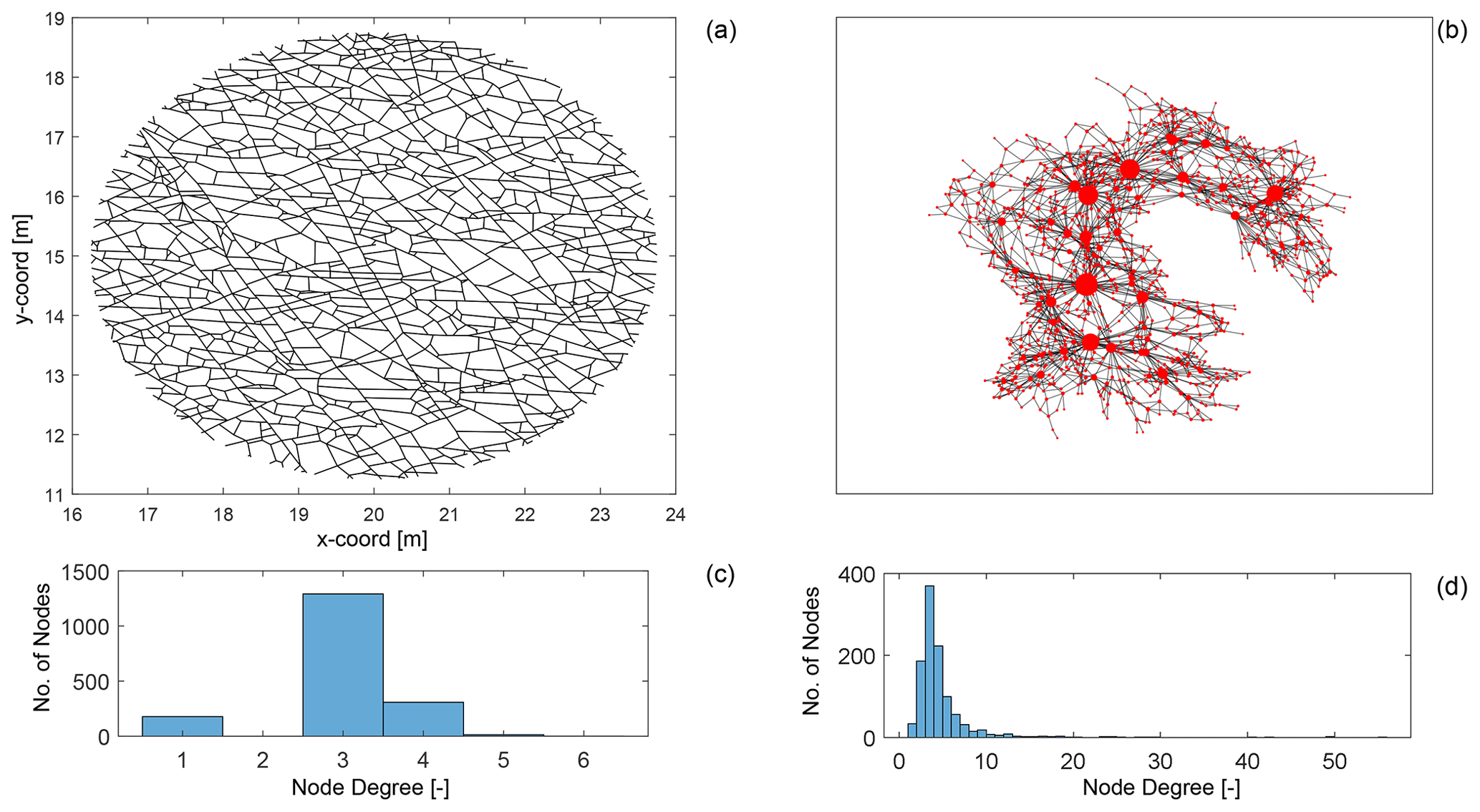
Figure 1 Comparing primal and dual forms of a fracture network from data published by Prabhakaran et al. (2021b): (a) a fracture network depicted in the primal form with dimensions in metres, (b) corresponding dual representation of the fracture network with node sizing proportional to dual graph node degree and plotted using a force layout, (c) node degree distribution of primal graph, and (d) node degree distribution of the dual graph.

We depict an example of a fracture network in its primal form (see Fig. 1a) and in its dual form (see Fig. 1b). The degree of a graph node is simply the number of edges that are incident at a particular node. As seen in the primal graph in Fig. 1c, the maximum node degree is 6, with the most common degree value being 3. This type of degree distribution is typical for a spatial graph in which physical constraints limit the maximum possible node degree. We may note that node degrees in spatial graph representations of fracture networks are most likely to be 1, 3, or 4. For fracture networks interpreted from outcrop images as depicted in Fig. 1a, eroded fractures and enlarged apertures may lead to higher degrees due to issues in resolving closely spaced nodes.

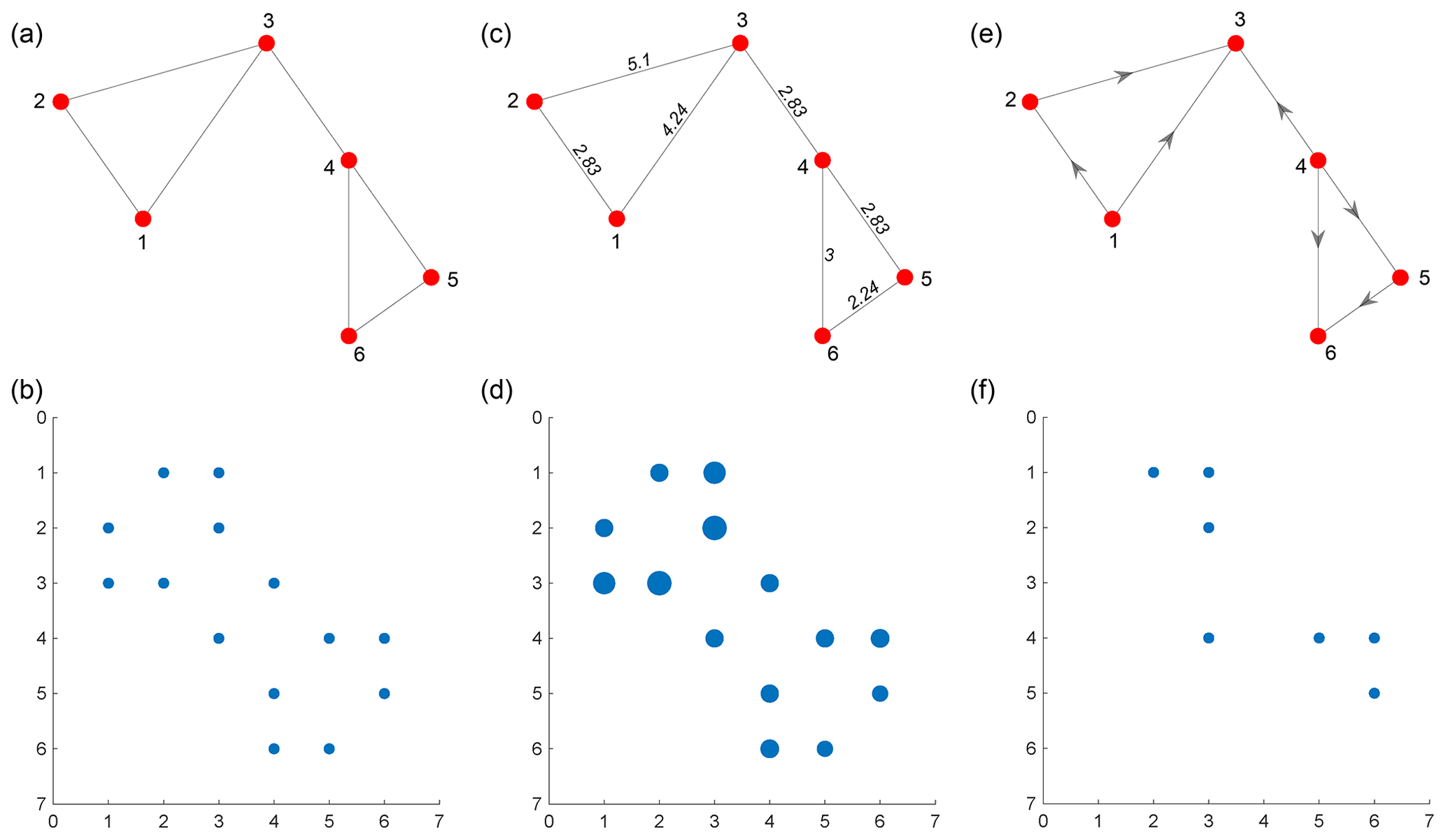
Figure 2 (a) An unweighted planar graph with six nodes and seven edges, (b) adjacency matrix of unweighted graph, (c) a weighted planar graph with edge weights proportional to Euclidean distances between connecting nodes, (d) weighted sparse adjacency matrix for weighted planar graph, (e) a directed, unweighted graph, and (f) adjacency matrix of directed graph.

In the case of the alternate representation, referred to as dual graphs by Barthelemy (2018) and depicted in Fig. 1d, the maximum degree can be much higher, and the longest fractures that have the highest number of intersections also have the highest degree. Andresen et al. (2013) and Vevatne et al. (2014) suggested that fracture networks are disassortative in that shorter fractures preferentially attach on to the longer fractures. The property of disassortativity is quantitatively defined using assortativity coefficients (Newman, 2002) with disassortative networks having negative assortativity coefficients. Andresen et al. (2013) and Vevatne et al. (2014) report negative assortativity coefficients for fracture networks that are represented in the dual form. Prabhakaran et al. (2021b) found such a correlation between dual graph node degree and length.

In graph representations, weights can be assigned to edges that are proportional to the importance of that edge. In the case of fracture networks in the primal form, this can be the Euclidean distance between the nodes (or fracture edge intersections). The weight may also be the direction cosine of the particular edge that indicates orientation. In the dual graph representation, intersections between fractures represent the edges. Therefore, the edge weight may be specified in terms of intersection angle. Graphs may also be directed with a specific direction to edges. In the case of spatial graphs derived from fracture networks, an undirected but weighted representation is sufficient. Figure 2a, c, and e depict examples of unweighted, weighted, and directed planar graphs, respectively. The corresponding adjacency matrices are depicted in Fig. 2b, d, and f.

2.2 Graph distance measures to quantify network similarity

Several graph similarity measures exist within the graph theory literature to compare graphs (see Hartle et al., 2020; Tantardini et al., 2019; Emmert-Streib et al., 2016, for recent reviews). Graph comparisons are a challenging, non-trivial problem in terms of computing complexity (Schieber et al., 2017). Still, various measures exist that can capture and highlight useful aspects of the graph structure that facilitate comparisons. Graph isomorphism between two graphs implies that there exists a series of necessary conditions such as an equal number of nodes, edges, degree sequences, and sufficient conditions such as equal adjacency matrices (Van Steen, 2010). An isomorphism test on two graphs, G₁ and G₂, can only yield two results, either isomorphic or not. Graph similarity can therefore be differentiated from graph isomorphism in that the latter comparison can only return a binary outcome. Graph similarity on G₁ and G₂, on the other hand, returns a real-valued quantity that converges to zero when the two graphs approach isomorphism (or complete similarity).

Tantardini et al. (2019) classify distance measures based on whether the metric is capable of comparing graphs with an unequal number of nodes or not. The metrics may also be classified based on whether they can also handle weighted and directed graphs. Using a graph similarity measure on a fracture network, we can explore spatial variations in network structure by comparing multiple sampling points.

2.3 Combining dissimilarity measures with clustering algorithms

Since we are interested in quantifying spatial variability, we may recast the problem as that of identifying clusters within the network. Clustering is also referred to as unsupervised classification and is a process of finding groups within a set of objects with an assigned measurement (Everitt et al., 2011). If we consider a dataset, $D=[X_{\mathrm{1}},X_{\mathrm{2}},\mathrm{\dots }{X}_n]$, containing “n” data samples, clustering then implies arranging the elements of D into “m” distinct subsets, $C=[C_{\mathrm{1}},C_{\mathrm{2}},\mathrm{\dots }{C}_m]$, where m≤n. From a statistical perspective, the clustering task is different from classification because the former is exploratory, whereas the latter is predictive, although both attempt to assign labels. Therefore, clustering must precede classification.

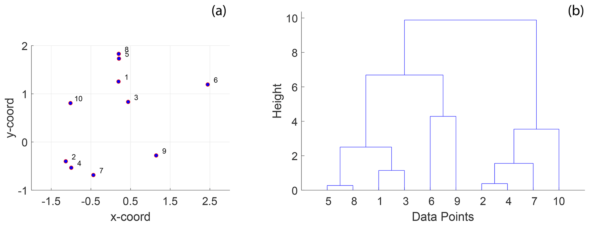
Figure 3 A simple example of hierarchical clustering using Euclidean distance: (a) 10 randomly positioned points in 2-D space and (b) a dendrogram computed from hierarchical clustering using the Euclidean distance depicting clusters of the 10 individual points at different levels organized into a hierarchy. The procedure of hierarchical clustering is shown in Algorithm 1.

In the existing literature on fracture networks, assigning labels to specific perceived archetypal networks (or end-members) is standard. These typologies include terms such as orthogonal, nested, ladder-like, conjugated, polygonal, corridors, etc. (Bruna et al., 2019a, b; Peacock et al., 2018). However, when faced with the reality of outcrop-derived 2-D fracture trace data, it is not easy to assign such labels. Therefore, clustering is a significant and necessary step in exploratory fracture data analysis.

Hierarchical clustering (HC) is an unsupervised statistical clustering method (Kaufman, 1990) that can identify clusters within a set of observations given a distance matrix computed by applying a well-defined distance function, pair-wise on each observation. In contrast to other clustering methods such as k means or k medoids, which require an a priori known number of clusters as input arguments, HC re-organizes observations into hierarchical representations from which the user can pick a level of granularity. At the lowest level, there is just one cluster containing all the observations. At the highest level, the number of clusters is equal to the observations. HC algorithms are referred to as “agglomerative” or “divisive” depending upon whether they begin from a lower level or from the highest level. The clustering then organizes the discrete data into a hierarchical dendrogram structure that positions the clusters based on the magnitude of similarity. By combining graph distance computations across spatially distinct samplings with unsupervised HC, cluster detection automatically leads to quantified spatial variation. A simple example of HC is illustrated on a set of randomly distributed points in space (see Fig. 3a). The result is the hierarchical dendrogram structure depicted in Fig. 3b.

3 Fracture datasets

To validate the proposed approach based on graph distance metrics and hierarchical clustering, we utilize a 2-D joint fracture dataset from the Lilstock pavement in the Bristol Channel, UK (Prabhakaran et al., 2021b). The dataset consists of fracture joints automatically traced using a technique described in Prabhakaran et al. (2019) from UAV photogrammetric data published by Weismüller et al. (2020). The joint networks correspond to Jurassic limestones with very dense joint networks spread across multiple layers. The joints are stratabound and perpendicular to bedding. We consider three large-scale fracture networks from this dataset, as depicted in Fig. 4. There is considerable spatial variation in the jointing. From previous literature documenting joints within the Lilstock pavements, the spatial variation is attributed to multiple reasons.

Figure 4 Overview of fracture networks corresponding to the three considered regions. This map is derived from an open image dataset published by Weismüller et al. (2020) and available for download with a CC-BY license.

The proposed explanations include proximity and influence of faults explained by fluid-driven radial-jointing emanating from asperities within fault (e.g. Rawnsley et al., 1998; Gillespie et al., 1993), spatial variation of thicknesses of intercalated limestone and shale layers (e.g. Belayneh, 2004), proximity to high-deformation features such as folding (e.g. Belayneh and Cosgrove, 2004), the interplay between regional and local stresses resulting in complex stress fields (e.g. Whitaker and Engelder, 2005), inheritance from the spatial distribution of pre-existing vein/stylolite networks that influenced later joint network development (e.g. Wyller, 2019; Dart et al., 1995), and synkinematic cementation in veins affecting later development of joints (Hooker and Katz, 2015). Recent work on fractures at the Kilve outcrop (Procter and Sanderson, 2018), exposing the same geological units as those considered in this work, concludes that anomalous fracture intensity exists in fracturing at various locations and suggest that variability in fracture intensity cannot be fully explained by variations in thickness, compositional, or textural variations.

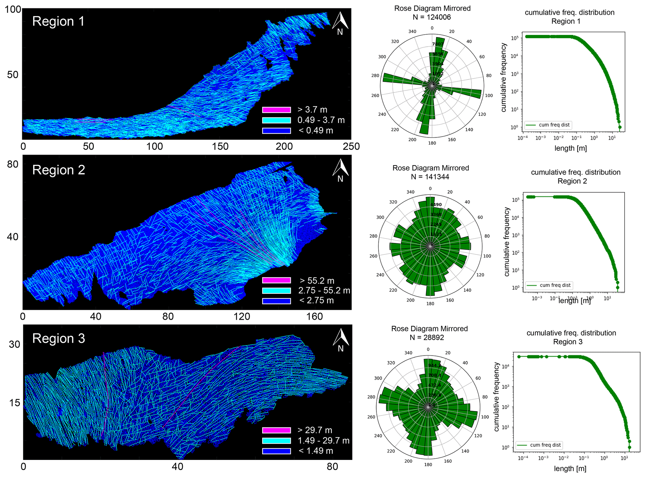
Figure 5 Comparison of the three regions in terms of networks, orientations, and length distributions. Map dimensions are in metres. This image has been modified from Prabhakaran et al. (2021b) with permission.

Table 1 Summary statistics for the three regions.

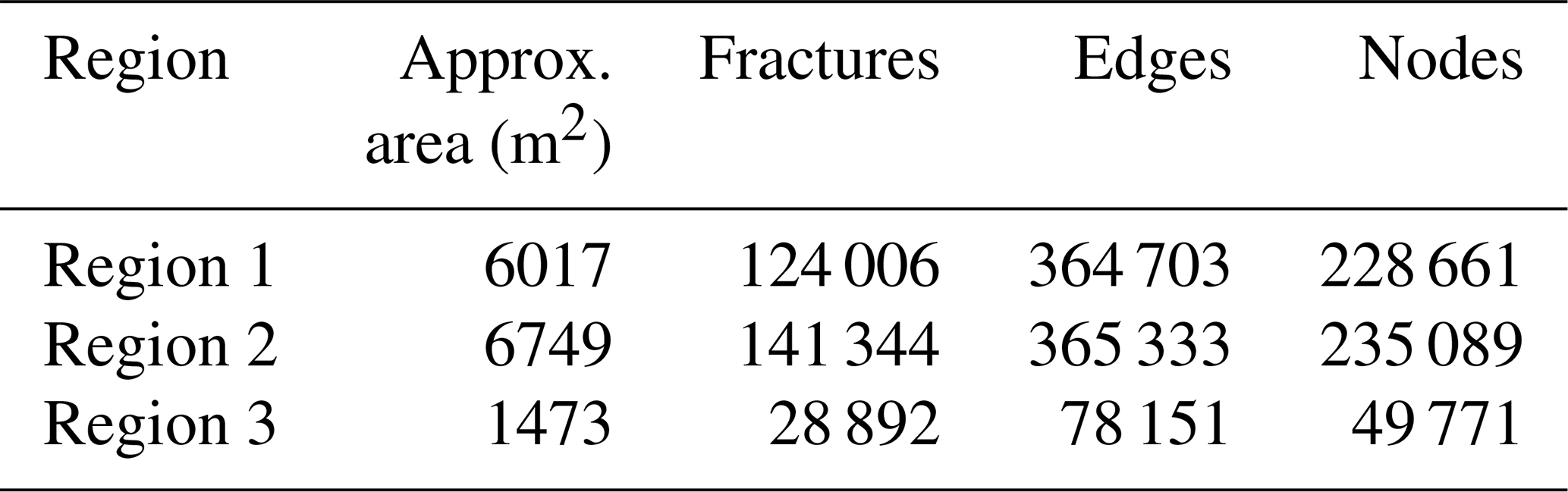
From this dataset, we utilize fracture networks corresponding to three contiguous regions. Figure 4 depicts the three areas' spatial extent, labelled as Regions 1 to 3. The intensity of fracturing is such that the spatial graphs corresponding to each region have a single connected component. Table 1 tabulates summary statistics for the three networks. The number of edges and nodes correspond to the primal graph representation. The “fractures” in Table 1 are sequences of graph edges that are clubbed together based on continuity and a strike direction threshold (or number of dual graph nodes). Regions 1 and 2 correspond to a single stratigraphic layer but, due to erosion, they are not contiguous within the outcrop. We treat them separately in our analysis of spatial variation.

The detailed resolution, topological accuracy, and spatial extent of the traced networks make the dataset appropriate for a detailed analysis of spatial variation in fracturing. The networks have significant intra- and inter-network variability in fracturing. Figures 5, 6, and 7 illustrate these differences. From Fig. 5, the fracture orientations of Region 1 depict discernable angular bins of fracture orientations. On the other hand, rose plots of Regions 2 and 3 show considerable scatter due to the presence of long and curved fractures. Fracture length distributions are different, with Region 2 having the longest fractures and Region 1 the shortest. The distribution of joints within a particular length bin is also highly variable. In Fig. 6, the cumulative variation in the strike along individual fracture edges that comprise a tip-to-tip fracture is plotted as a function of the total length. The slope of the scatter plots gives an indication of the fracture curvature. The slope of the scatter plot is higher in Regions 2 and 3 than in Region 1. We interpret the curvature to therefore be the lowest in Region 1.

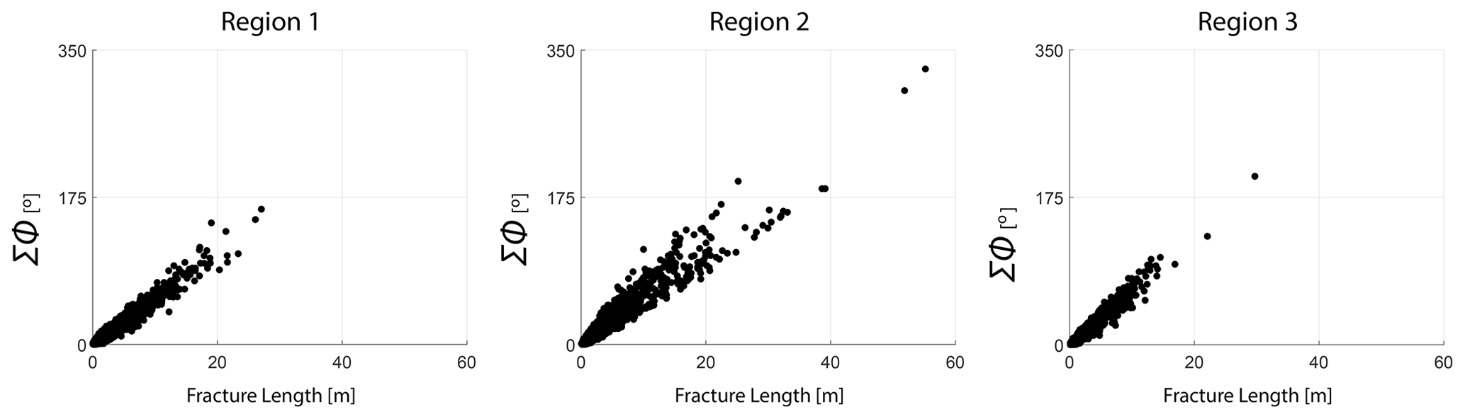
Figure 6 Correlation between sum of strike differences of fracture segments constituting tip-to-tip fractures versus total fracture length for the three regions.

Figure 7 Cutout from Region 2 depicting the detailed resolution of the fracture dataset.

4 Methods

4.1 Subsampling the network data

We circularly sample the fracture networks on a cartesian grid with a subgraph extracted within a circular region centred at each grid point. The grid spacing to circle diameter is maintained such that neighbouring subgraphs share some portion of the area (see Fig. 8). Near the networks' boundaries, the subgraphs are either too small or result in disconnected graph components. We neglect these samples so that they do not affect the clustering results. The process of circular sampling creates edge nodes with degree 1, which has the effect of altering node topology by introducing isolated, degree-1 nodes. To prevent this from impacting clustering results, we remove all edges from the subgraphs emanating from degree-1 nodes that contact the periphery of the circular sample. This effect is illustrated in Fig. 9. Each subgraph can now be compared to every other subgraph using a graph distance metric to compute a pair-wise distance matrix. The distance matrix serves as the input to the hierarchical clustering algorithm.

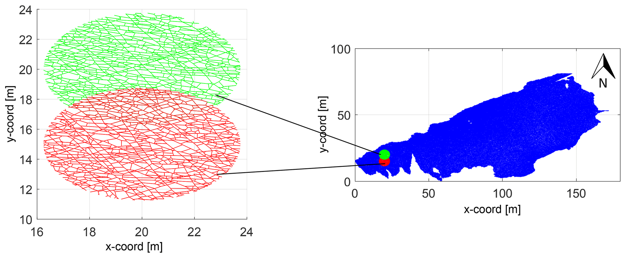
Figure 8 Subsampling of a fracture graph corresponding to full region into subgraphs of 7.5 m diameter and spacing of 5 m.

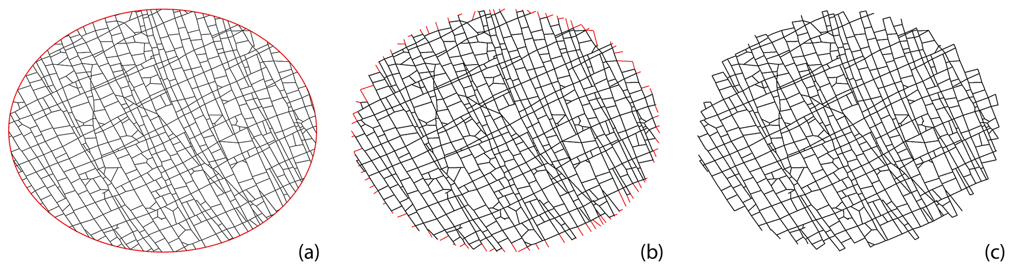
Figure 9 Treating isolated nodes and dangling edges that arise due to circular sampling: (a) a circularly sampled subgraph with a diameter of 7.5 m, (b) edges connected to isolated nodes intersected by circle, and (c) subgraph after removing isolated nodes and corresponding dangling edges.

Table 2 Number of subgraphs obtained per region.

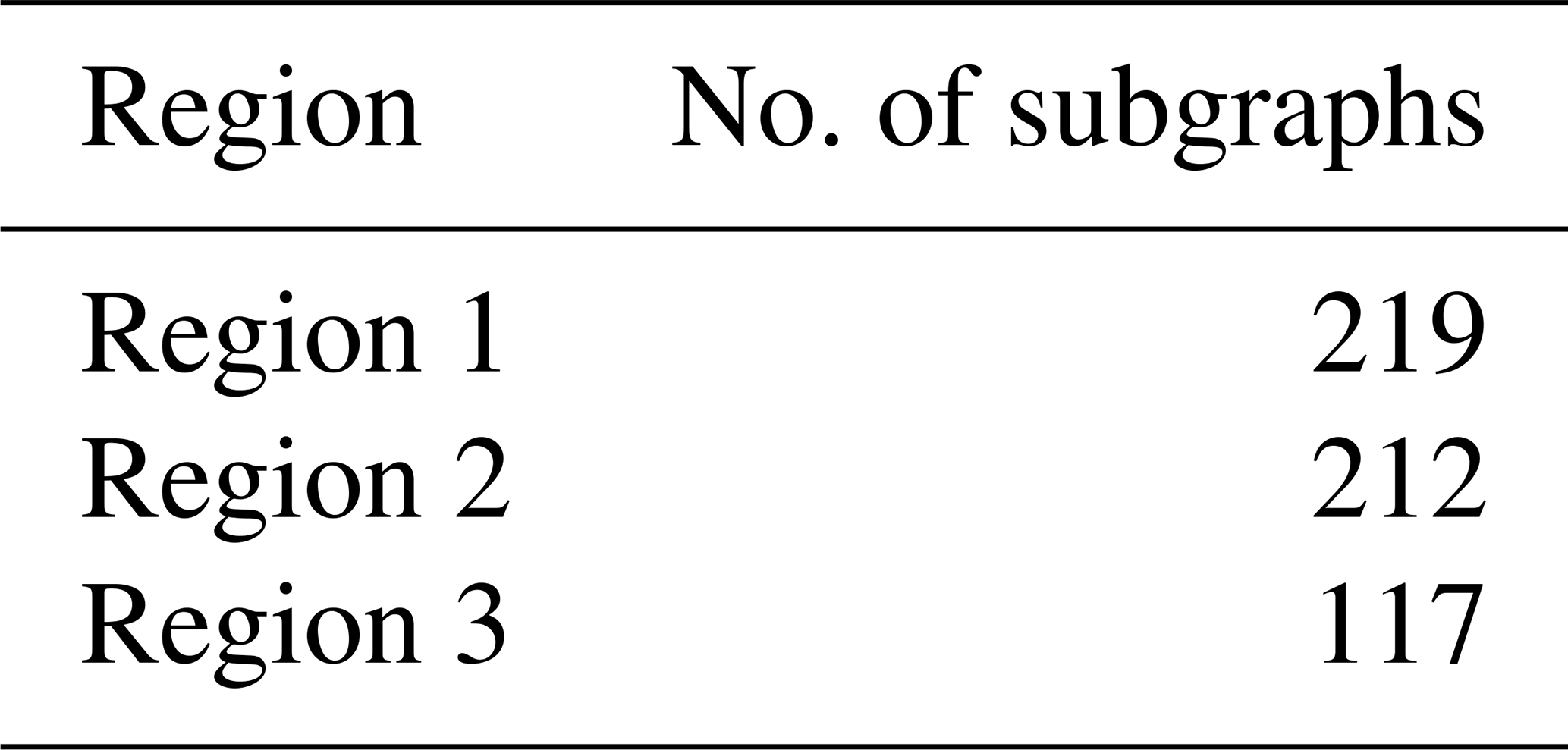
For N subgraphs, the number of comparisons necessary are $\frac{N(N-\mathrm{1})}{\mathrm{2}}$. The computational complexity of graph comparison increases polynomially with the size of subgraphs in terms of node sizes. Since the number of comparisons increases quadratically with the number of subgraphs, we seek to balance grid spacing and sampling diameter. For Regions 1 and 2, we choose a spacing of 5 km for circularly sampled subgraphs with a diameter of 7.5 m. For Region 3, which is also the smallest region, a spacing of 5 km would lead to quite a smaller number of subgraphs. Therefore, we use a more dense spacing of 3 km with a diameter of 7.5 m. Table 2 tabulates the number of subgraphs pertaining to each region.

4.2 Graph similarity measures

We use the following four graph similarity measures to compare the subgraphs:

• fingerprint distance (Louf and Barthelemy, 2014);

• D-measure (Schieber et al., 2017);

• Network Laplacian spectral descriptor (NetLSD) (Tsitsulin et al., 2018);

• portrait divergence (Bagrow and Bollt, 2019).

The performance of these similarity measures have been validated previously by Hartle et al. (2020) and Tantardini et al. (2019) for a variety of benchmark graph datasets. Each similarity measure is described briefly in the following subsections. The reader is referred to the references above for further details on the similarity measures.

4.2.1 Fingerprint distance

The fingerprint distance introduced by Louf and Barthelemy (2014) is purely geometric and combines statistics of block faces and shape factors in computing a probability distribution of a spatial graph. Louf and Barthelemy (2014) formulated the measure in the context of quantifying differences in street patterns. A “block” denotes the 2-D region enclosed by graph edges. For any given spatial graph, this corresponds to the number of bounded subgraphs or primary cycles. We neglect isolated fractures and those having dead ends when computing these blocks. Given the network intensity in our dataset, such isolated fractures are minimal. Every block has an associated shape factor, “ϕ” which is expressed in terms of block area “A” and circumscribing circle area, “A_c”:

$$\begin{array}{}\text{(1)}& {\displaystyle }{\displaystyle }\mathit{\varphi }={\displaystyle \frac{A}{A_{\mathrm{c}}}}.\end{array}$$

The value of ϕ is always smaller than 1, with larger values meaning that the block-face shape is closer to that of a regular polygon. Figure 10a depicts shape factors of regular polygons versus that of polygons derived from spatial networks in Fig. 10b. No unique correspondence exists between a particular shape and a magnitude of ϕ; however, the overall distribution of ϕ indicates reveals block shape distribution patterns and highlights differences between spatial graphs. The shape factor alone does not fully serve as a similarity measure as blocks can have similar shapes but different face areas. The distribution of the block-face areas is binned logarithmically to integrate information from the shape factor and block area distributions. A conditional probability distribution, P(ϕ|A)P(A), is then defined representing the contribution of P(ϕ) for each area bin and the summation of which yields the fingerprint curve, P(ϕ):

$$\begin{array}{}\text{(2)}& {\displaystyle }{\displaystyle }P\left(\mathit{\varphi }\right)=\sum _{A}P\left(\mathit{\varphi }\right|A\left)P\right(A).\end{array}$$

An example of a “fingerprint”, so named by Louf and Barthelemy (2014), is depicted in Fig. 11e and j, with the distribution curves for three area bins, for two fracture networks derived from image tiles (see Fig. 11b, c, f, and g) corresponding to Region 1 (Fig. 11a). The curves in Fig. 11e and j encapsulate information based on shape factors and block areas (see Fig. 11d and h), including the proportional contribution from all logarithmic area bins considered.

Figure 10 (a) Shape factors for regular block shapes with equal edge lengths and (b) shape factors for polygonal blocks resulting from real fracture networks in Region 1 (dimensions are relative).

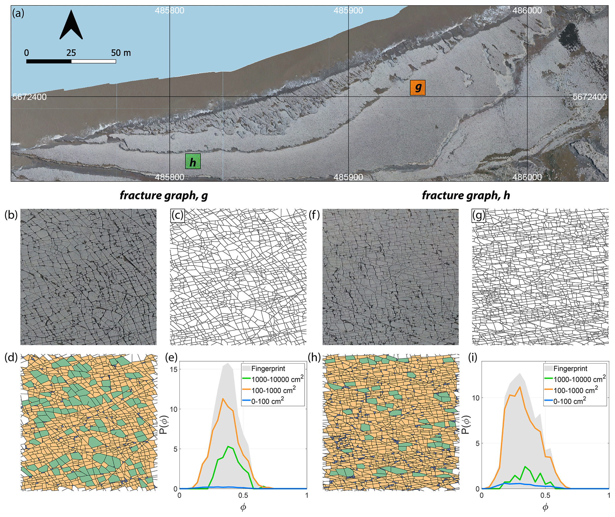
Figure 11 (a) Overview of Region 1 with two selected 1000×1000 pixel image tiles, (b) enlarged view of first image tile, (c) fracture network corresponding to first tile as a spatial graph with dimensions of 8.6 m×6.75 m and having 3583 edges and 2382 nodes, (d) block-face areas coloured as per three area bins (0–100, 100–1000, and 1000–10 000 cm²), (e) P(ϕ) or fingerprint of the subgraph depicting the combined effects of area and shape factor, ϕ pertaining to the three area bins. (f) Enlarged view of second image tile, (g) fracture network corresponding to second image tile as a spatial graph with 5418 edges and 3539 nodes, (h) block-face areas binned logarithmically, and (i) fingerprint of second spatial graph. Panels (a, b), and (f) are derived from images contained in the open dataset (CC-BY license) published by Weismüller et al. (2020).

Denoting f_α(ϕ) as the ratio of the number of faces with a shape factor “ϕ” that lie in a bin “α” over the total number of faces for that graph, a distance d_α between two graphs G_a and G_b is computed by integrating over f_α(ϕ) for the two different graphs. The distance based on f_α(ϕ) of the two graphs for a single area bin is defined as

$$\begin{array}{}\text{(3)}& {\displaystyle }{\displaystyle }{d}_{\mathit{\alpha }}(G_a,G_b)=\underset{\mathrm{0}}{\overset{\mathrm{1}}{\int }}{\left|f_{\mathit{\alpha }}^a\left(\mathit{\varphi }\right)-f_{\mathit{\alpha }}^b\left(\mathit{\varphi }\right)\right|}^n\mathrm{d}\mathit{\varphi }.\end{array}$$

As per Louf and Barthelemy (2014), the value of n can either be 1 or 2. We choose n=1 in our computation. The global fingerprint distance D_FP between G_a and G_b can then be computed summing over all area bins α:

$$\begin{array}{}\text{(4)}& {\displaystyle }{\displaystyle }{D}_{\text{FP}}(G_a,G_b)=\sum _{\mathit{\alpha }}{d}_{\mathit{\alpha }}(G_a,G_b{)}^{\mathrm{2}}.\end{array}$$

We have attached our MATLAB implementation of the fingerprint distance in the code Supplement. We computed the distance matrix for all subgraphs corresponding to the three regions using this implementation.

4.2.2 D-measure

The D-measure introduced by Schieber et al. (2017) is a three-component distance metric with weighting constants for each component. The three properties of graphs compared are the network node dispersion (NND), node distance distribution (μ), and the alpha (α) centrality. The dissimilarity measure, D_DM, is the weighted sum:

$$\begin{array}{ll}{\displaystyle }{D}_{\text{DM}}(g,h)=& {\displaystyle }{w}_{\mathrm{1}}\sqrt{{\displaystyle \frac{\mathcal{J}({\mathit{\mu }}_g,{\mathit{\mu }}_h)}{\log \mathrm{2}}}}\\ {\displaystyle }& {\displaystyle }+w_{\mathrm{2}}\left|\sqrt{\text{NND}\left(g\right)}-\sqrt{\text{NND}\left(h\right)}\right|\\ {\displaystyle }& {\displaystyle }+{\displaystyle \frac{w_{\mathrm{3}}}{\mathrm{2}}}\left(\sqrt{{\displaystyle \frac{\mathcal{J}\left(P_{\mathit{\alpha }}\right(g),P_{\mathit{\alpha }}(h\left)\right)}{\log \mathrm{2}}}}\right.\\ \text{(5)}& {\displaystyle }& {\displaystyle }\left.+\sqrt{{\displaystyle \frac{\mathcal{J}\left(P_{\mathit{\alpha }}\right(g^c),P_{\mathit{\alpha }}(h^{c^{\prime }}\left)\right)}{\log \mathrm{2}}}}\right),\end{array}$$

where 𝒥 indicates the Jensen–Shannon divergence. The constants w₁, w₂, and w₃ in Eq. (5) are real and non-negative weights such that $w_{\mathrm{1}}+w_{\mathrm{3}}+w_{\mathrm{3}}=\mathrm{1}$.

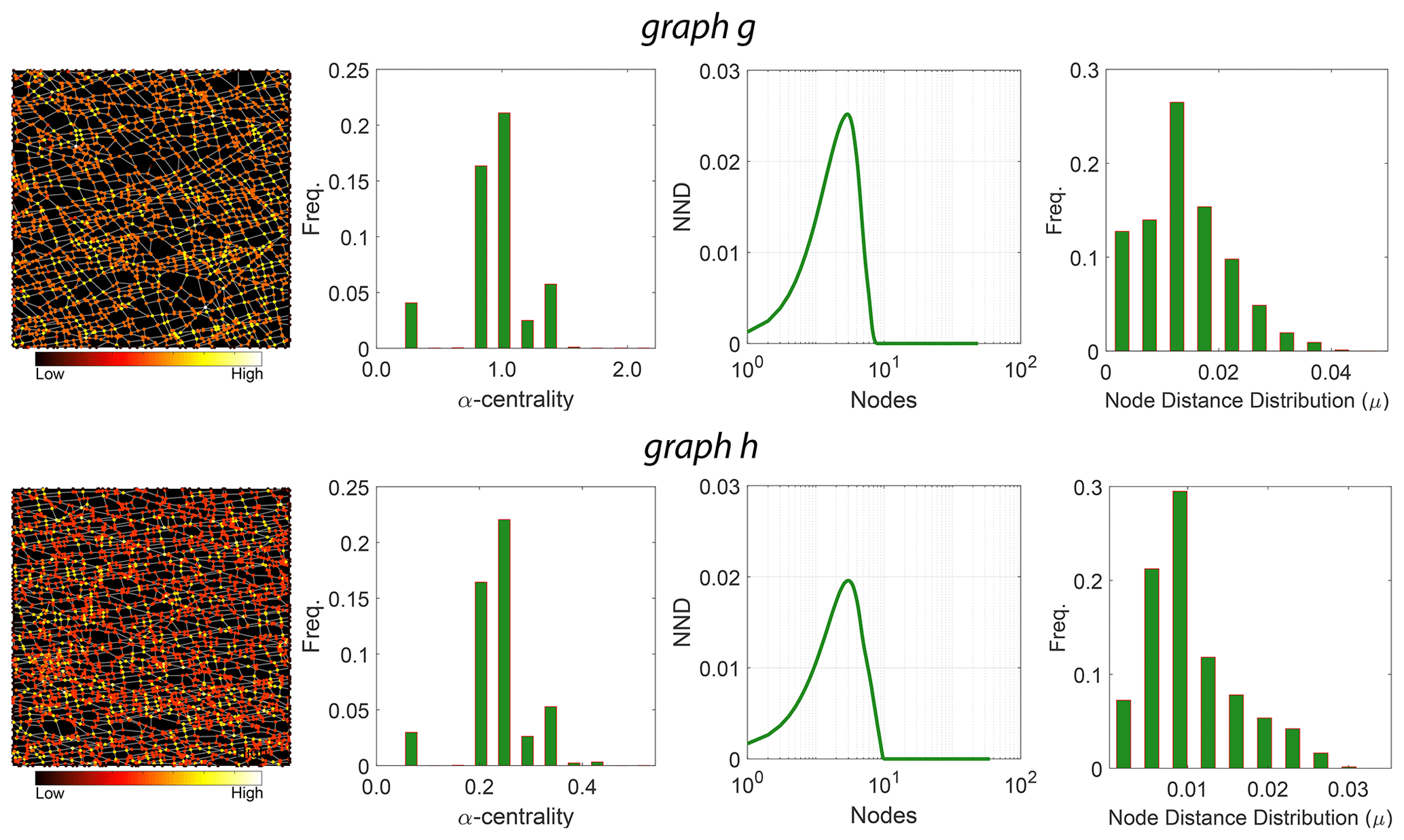
Figure 12 D-measure components for the two example fracture graphs comparing α centrality of nodes, distributions of α centrality, NND distributions, and node distance distributions.

As per Schieber et al. (2017), the first term in Eq. (5) compares averaged connectivity node's patterns as per node distance distribution. Schieber et al. (2017) define NND, within the second term, as a measure of the heterogeneity of a graph with respect to connectivity distances that capture global topological differences. The NND is computed as

$$\begin{array}{}\text{(6)}& {\displaystyle }{\displaystyle }\text{NND}\left(G\right)={\displaystyle \frac{\mathcal{J}(P_{\mathrm{1}},\mathrm{\dots },P_N)}{\log (d+\mathrm{1})}},\end{array}$$

where the numerator in Eq. (6) is the Jensen–Shannon divergence of N connectivity distance distributions [P₁,P₂…P_N]. P_i is constructed as P_i=p_i(j), where p_i(j) is the fraction of nodes connected to node i at distance j. The Jensen–Shannon divergence of [P₁,P₂…P_N] is expressed as

$$\begin{array}{}\text{(7)}& {\displaystyle }{\displaystyle }\mathcal{J}(P_{\mathrm{1}},\mathrm{\dots },P_N)={\displaystyle \frac{\mathrm{1}}{N}}\sum _{i,j}{p}_i\log \left({\displaystyle \frac{p_i\left(j\right)}{{\mathit{\mu }}_j}}\right).\end{array}$$

μ_j in Eq. (7) is the average of N distributions and can be written as

$$\begin{array}{}\text{(8)}& {\displaystyle }{\displaystyle }{\mathit{\mu }}_j={\displaystyle \frac{\mathrm{1}}{N}}\sum _{i=\mathrm{1}}^N{p}_i\left(j\right).\end{array}$$

The third term in Eq. (5) is based on probability density functions associated with α centrality of graph P_α(g) and α centrality of the graph complement P_α(g^c). The value of weights was suggested by Schieber et al. (2017) as $w_{\mathrm{1}}=w_{\mathrm{2}}=\mathrm{0.45}$ and w₃=0.1. We use the implementation provided by Schieber et al. (2017) with these sets of weights to build the distance matrices for all subgraphs within the three regions of interest. We depict in Fig. 12, for the two example fracture networks, the three properties that are used in computing the D-measure.

4.2.3 Portrait divergence

The portrait divergence similarity score derives from network portraits introduced by Bagrow et al. (2008) for unweighted graphs and extended to weighted graphs by Bagrow and Bollt (2019). For a graph g with N nodes, the network portrait is defined as a matrix B_lk, where each entry is the number of nodes with k nodes at l distance. The limits of l and k are $\mathrm{0}\le l\le d$ and $\mathrm{0}\le k\le N-\mathrm{1}$, with d being the diameter of the graph. The row entries of the network matrix B_lk are probability distributions of a random node having k nodes at a distance l:

$$\begin{array}{}\text{(9)}& {\displaystyle }{\displaystyle }P\left(k\right|l)={\displaystyle \frac{B_{lk}}{N}}.\end{array}$$

For a second graph h, if the network matrix is $B_{lk}^{\prime }$ with a corresponding probability distribution of Q(k|l) and diameter d^′, the Kullback–Leibler (KL) divergence between P(k|l) and Q(k|l) is expressed as

$$\begin{array}{}\text{(10)}& {\displaystyle }{\displaystyle }\text{KL}\left(P\right(k\left|l\right)\left|\right|P\left(k\right|l\left)\right)=\sum _{l=\mathrm{0}}^{max(d,d^{\prime })}\sum _{k=\mathrm{0}}^{N}P(k,l)\log {\displaystyle \frac{P(k,l)}{Q(k,l)}}.\end{array}$$

The portrait divergence D_PD(g,h) is computed by the Jensen–Shannon divergence between P(k|l) and Q(k|l):

$$\begin{array}{}\text{(11)}& {\displaystyle }{\displaystyle }{D}_{\text{PD}}(g,h)=\text{JSD}\left(P\right(k\left|l\right),Q\left(k\right|l).\end{array}$$

This can be expressed in terms of Kullback–Leibler divergences and mixture distributions as

$$\begin{array}{}\text{(12)}& {\displaystyle }{\displaystyle }{D}_{\text{PD}}(g,h)={\displaystyle \frac{\mathrm{1}}{\mathrm{2}}}\left(\text{KL}\right(P\left|\right|M)+\text{KL}(Q\left|\right|M\left)\right),\end{array}$$

where the mixture distribution M of P(k|l) and Q(k|l) is given by

$$\begin{array}{}\text{(13)}& {\displaystyle }{\displaystyle }M={\displaystyle \frac{\mathrm{1}}{\mathrm{2}}}\left(P\right(k\left|l\right)+Q\left(k\right|l\left)\right).\end{array}$$

The portrait divergence measure provides a single value $\mathrm{0}\le D_{\text{PD}}(g,h)\le \mathrm{1}$ for any pair of graphs. Bagrow and Bollt (2019) applied the portrait divergence measure to both synthetic and real-world networks. The code implementation of portrait divergence attached with Bagrow and Bollt (2019) is used to construct the distance matrices for all subgraphs within the three regions of interest. The network portrait or the B_lk matrix for the example fracture graphs are depicted as heatmaps in Fig. 13.

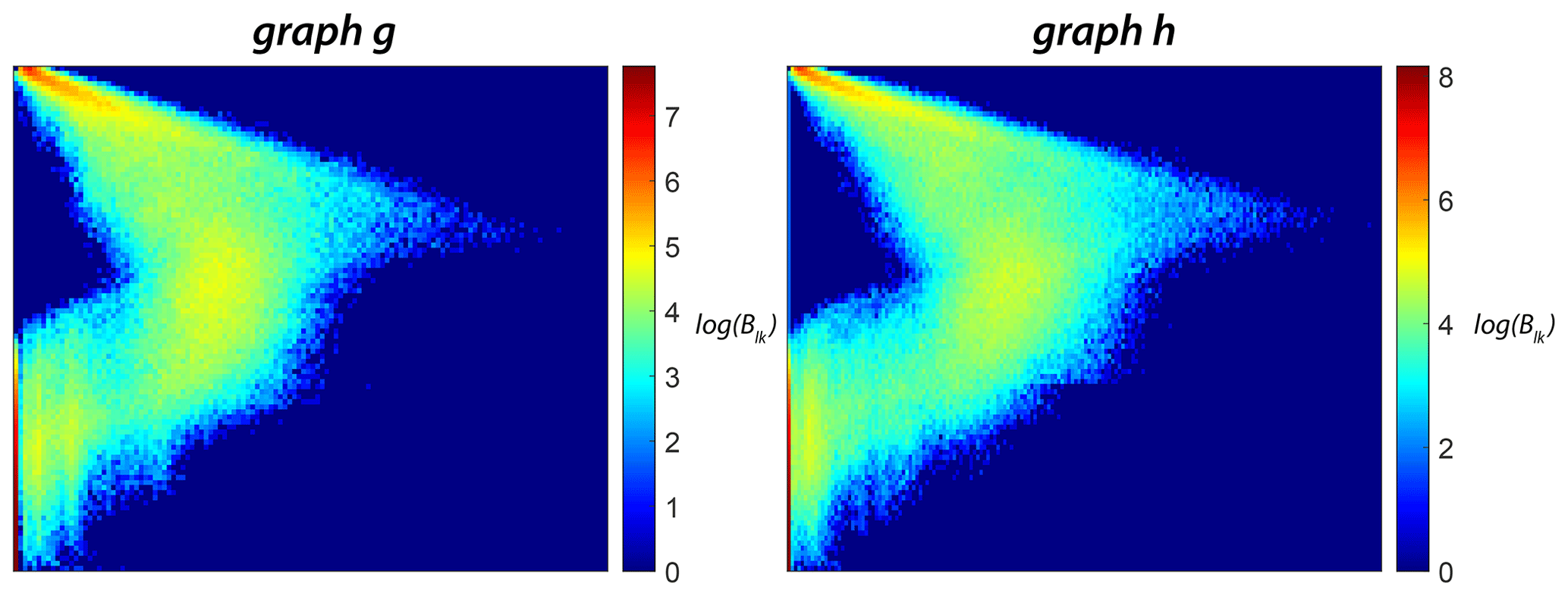
Figure 13 Heatmap representations of network portrait sparse matrices (B_lk) for the two example fracture graphs.

4.2.4 Laplacian spectral descriptor

The NetLSD distance was introduced by Tsitsulin et al. (2018). It is based on a Frobenius norm computed between heat trace signatures of normalized Laplacian matrices of two graphs. For a graph g with a normalized Laplacians L and n nodes, a heat kernel matrix is defined as

$$\begin{array}{}\text{(14)}& {\displaystyle }{\displaystyle }{\mathbf{H}}_{\mathrm{t}}=e^{-tL}=\sum _{j=\mathrm{1}}^n{e}^{-t{\mathit{\lambda }}_j}{\mathit{\varphi }}_j{\mathit{\varphi }}_j^{\mathrm{T}}.\end{array}$$

Using the heat kernel matrix H_t, a heat trace h_t is defined as

$$\begin{array}{}\text{(15)}& {\displaystyle }{\displaystyle }{h}_{\mathrm{t}}=\sum _{j=\mathrm{1}}^n{e}^{-t{\mathit{\lambda }}_j}.\end{array}$$

For a second graph g^′ with a heat trace signature of $h_{\mathrm{t}}^{\prime }$, the NetLSD distance D_LSD is then the Frobenius norm of the two heat signatures as

$$\begin{array}{}\text{(16)}& {\displaystyle }{\displaystyle }{D}_{\text{LSD}}=\left|\right|h_{\mathrm{t}},h_{\mathrm{t}}^{\prime }|{|}_{\text{Frobenius}}.\end{array}$$

Figure 14 depicts heat trace signatures computed using the NetLSD Python package implemented by Tsitsulin et al. (2018) for the two example fracture graphs. We use this package to populate the distance matrices associated with subgraphs from each region.

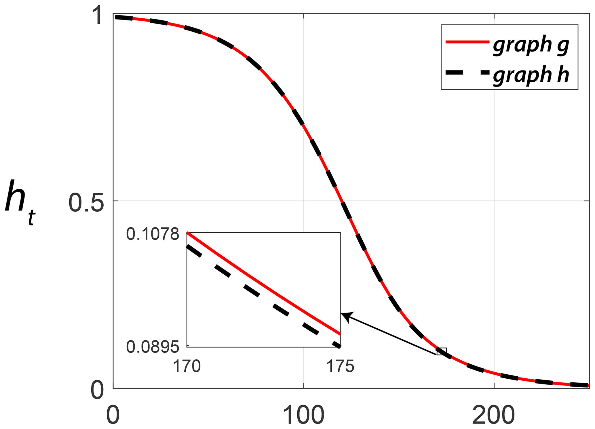
Figure 14 Comparing heat trace signature vectors for the two example fracture graphs computed using NetLSD.

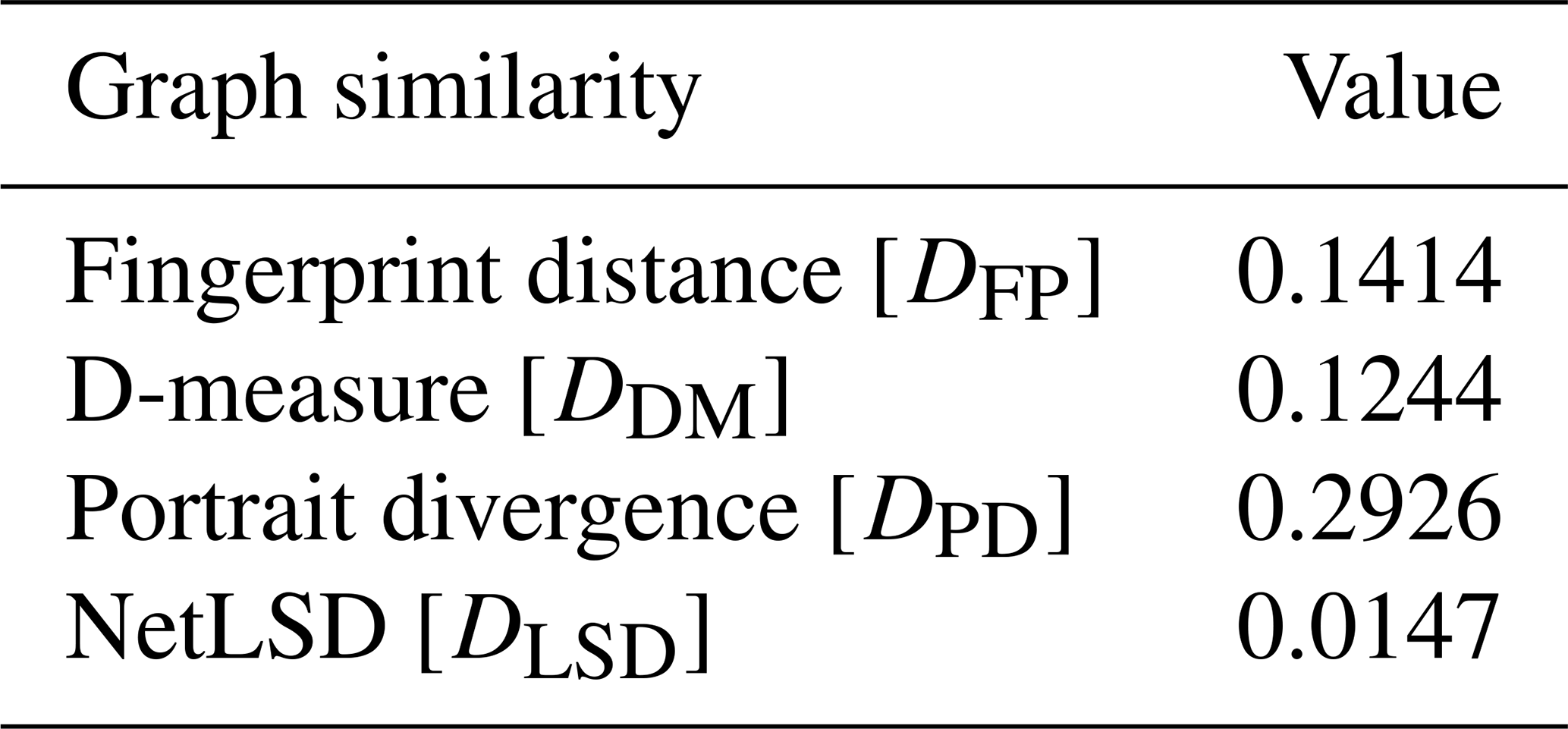
The values of graph similarity computed using the four metrics described by Eqs. (4), (5), (12), and (16) for the two example fracture graphs depicted in Fig. 11c and g are summarized in Table 3.

Table 3 Summary of graph similarities computed for example fracture networks.

4.3 Hierarchical clustering

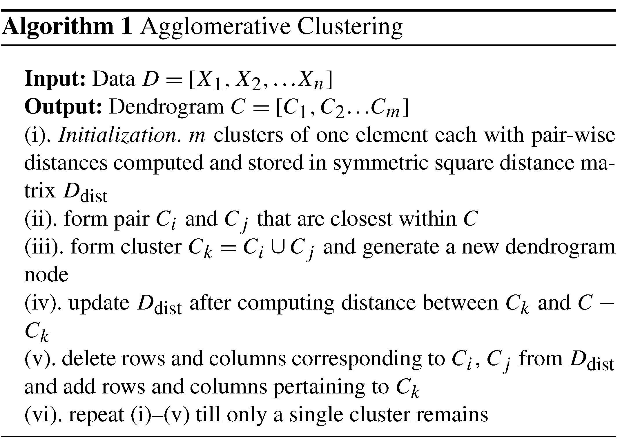
After subsampling the fracture networks (see Sect. 4.1) and using the graph distance metrics described in Sect. 4.2 to construct distance matrices, we apply hierarchical clustering. HC can be done in an agglomerative versus divisive manner (Hennig et al., 2016). We utilize the agglomerative approach, which generally follows the steps described in Algorithm 1. Based on how linking of clusters is done as per Algorithm 1(iii), HC can be classified into methods such as single linkage, complete linkage, unweighted pair-group average, weighted pair-group average, unweighted pair-group centroid, weighted pair-group centroid, and Ward's method (Wierzchoń and Kłopotek, 2018). Ward's method performs the linkage by minimizing the sum of squares of distances between objects and cluster centres. We use Ward's method implemented within the R statistical programming environment to apply the HC to all the subgraph distance data.

5 Results

We first show region-wise results of graph property computations. Intra-region spatial clustering resulting from the combined application of graph similarity measures with HC is then discussed. We use the following abbreviations for brevity throughout the section: FP – fingerprint distance, DM – D-measure, LSD – NetLSD, PD – portrait divergence.

5.1 Region-wise graph characteristics

Fingerprints pertaining to the regions are depicted in Fig. 15a. The peak of the fingerprint plot is highest at a shape factor of 0.4 for Region 1 and increases to above 0.5 for Regions 2 and 3. Histograms in Fig. 15a depict the number of polygons within each area bin pertaining to fracture networks in each region. The network portraits or B_lk matrices of each subgraph within the three regions are combined to create ensemble region-wise network portraits depicted as heatmaps in Fig. 15b. The non-zero entries in the B_lk matrices, indicated by warmer colours in the heatmaps, have visibly different patterns. Heat traces for the subgraphs in each region are shown in Fig. 15c. Figure 16 depicts the variation of the network properties that are components of the D-measure distance, i.e. α centrality, NND, and μ for subgraphs for the three regions.

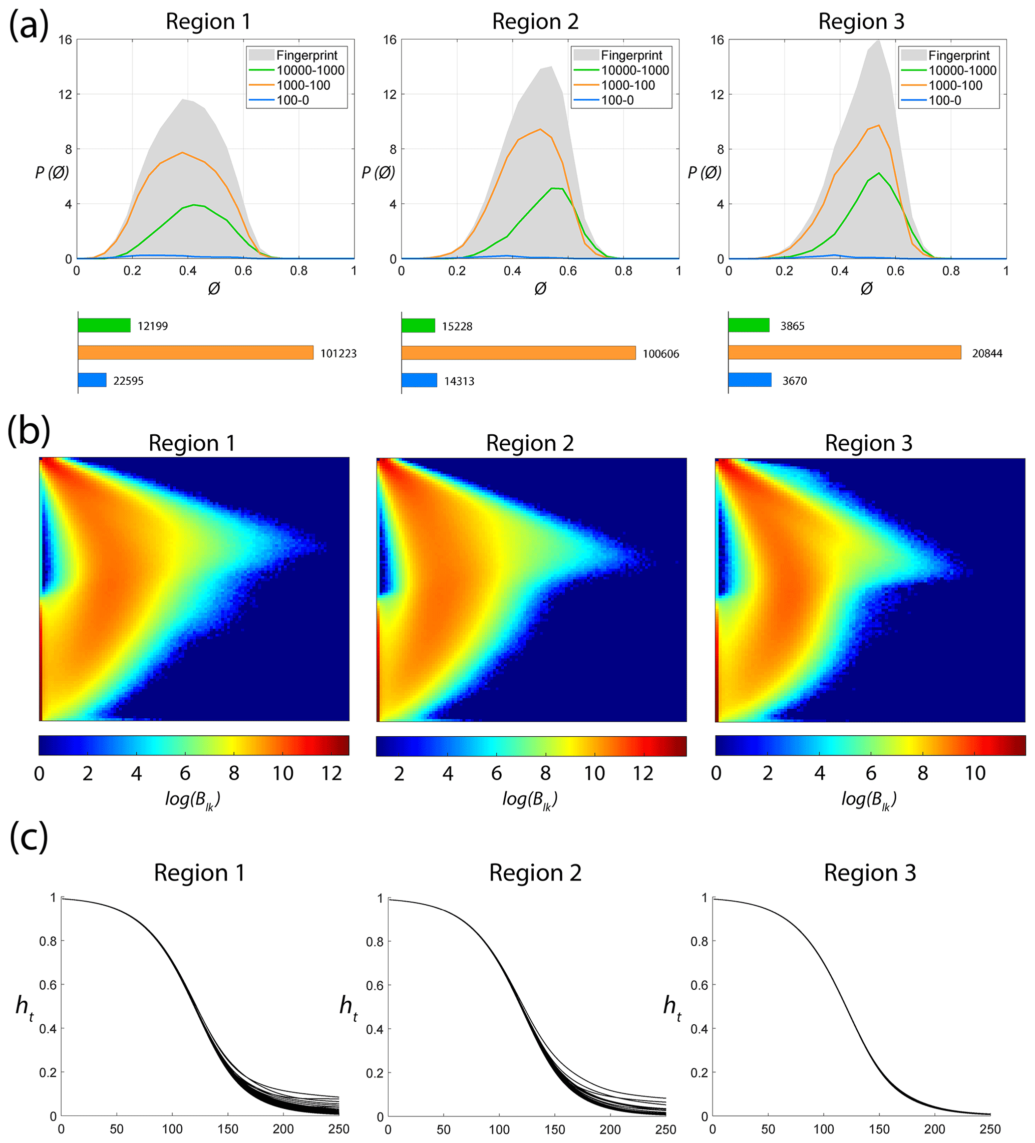
Figure 15 Region-wise graph properties: (a) fingerprints, (b) network portrait ensembles, and (c) heat trace vectors.

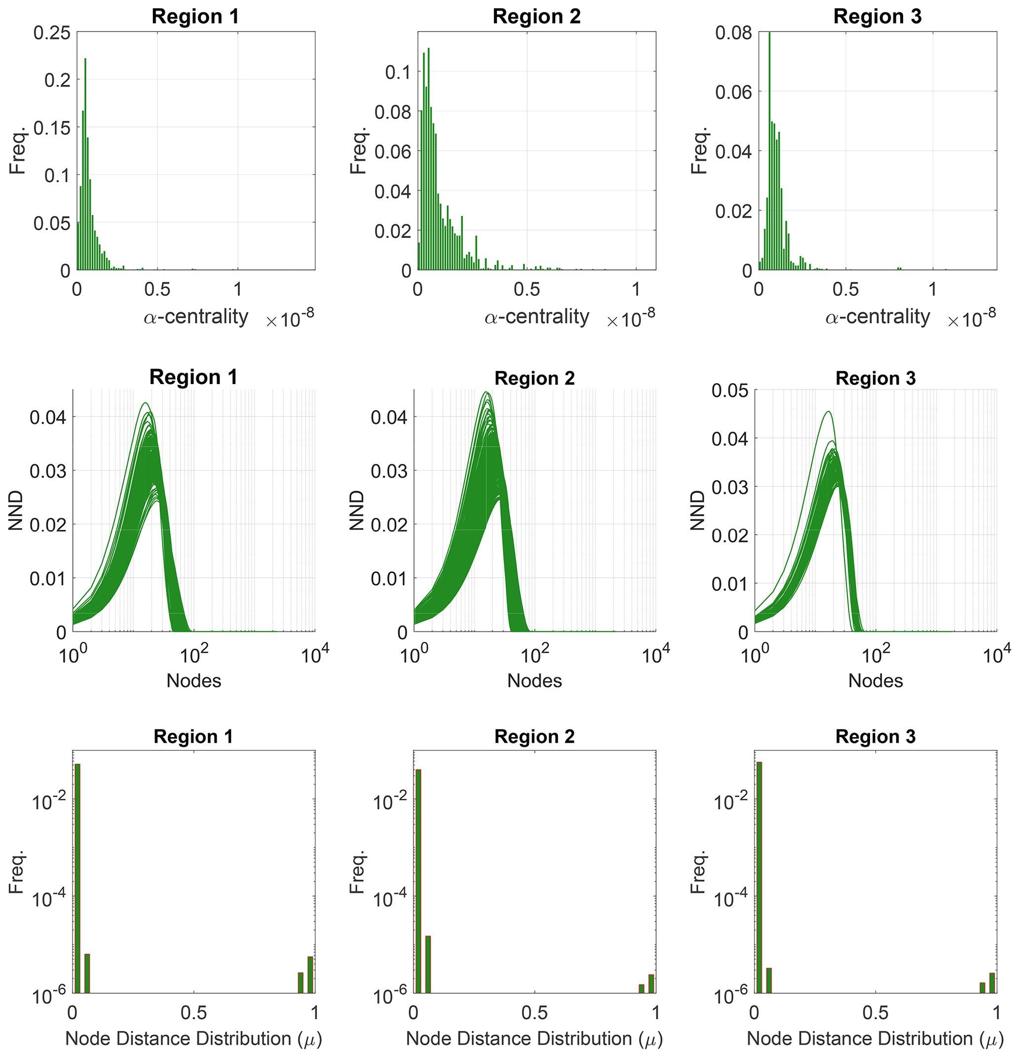
Figure 16 Region-wise properties used to compute the D-measure represented as ensemble plots of α centrality, network node dispersion (NND), and node distance (μ) distributions for subgraphs.

5.2 Intra-region spatial variation

Intra-region spatial variation results can be presented as distance matrix heatmaps corresponding to each graph similarity metric. Dendrograms depict the hierarchical organization of the subgraphs corresponding to similarity entries within the distance matrix entries. The intra-regional variation is more intuitively illustrated spatially by showing subgraphs using an appropriate colour scheme that groups similar clusters under colours picked within a linear spectrum. This section presents the clustering results for all three regions using a combination of dendrograms, spatial cluster maps, and heatmaps.

5.2.1 Analysis of spatial variation in Region 1

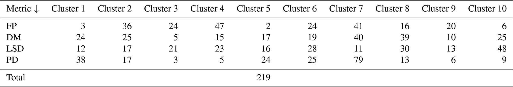
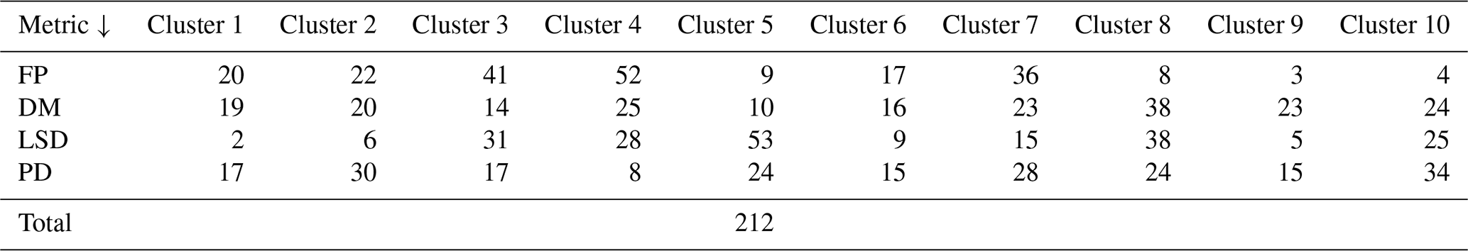
The spatial distribution of clusters pertaining to the four distance metrics overlain over the network is shown in Fig. 17a–d along with the associated dendrograms for the top 10 clusters. The subgraphs are represented by coloured discs that follow a diverging colour scheme. The number of subgraphs within each of the top 10 clusters is also listed under the dendrogram branches. It may be noted that the top 10 clusters are shown to depict, analyse, and compare the spatial variation across distance measures. A complete, uncut dendrogram and associated heatmaps of the similarity measures are depicted in Fig. A1 in the Appendix. We can cut the dendrogram at different heights guided by slope changes in the weighted sum of squares plots shown in Fig. A1. The boundaries of spatial clusters vary with the dendrogram cut height, with subregions emerging by traversing deeper into the dendrogram. This variation is depicted in Figs. B1–B4 in the Appendix for a range of clusters varying from 5–10. The number of subsamples for the four similarity measures pertaining to a dendrogram cut of k=10 is tabulated in Table 4.

Table 4 Summary of subgraphs within each cluster of Region 1 for k=10.

We can observe that spatial autocorrelation exists for the FP (Fig. 17a), DM (Fig. 17b), and PD (Fig. 17d) similarity measures. The LSD yields a speckled pattern with no obvious spatial autocorrelation (Fig. 17c). In order to compare clustering results derived from the graph similarity measures, the spatial fracture persistence P₂₀ and P₂₁ computed using box counting (box size of 0.5×0.5 m) is depicted in Fig. 17e and f, respectively. Comparing clusters derived from graph similarity measures to the fracture persistence plots reveals boundaries within the network that are not easily discernable from the latter. Since LSD does not show spatial autocorrelation, we do not analyse it further.

Figure 18a–c depict topology histograms and rose plots of the clusters pertaining to the remaining three similarity measures. The orientation rose plots and topological summaries are generated by combining all circular samples identified under a cluster into 10 cluster subgraphs from the larger region fracture graph. It can be observed from the rose plots that the clusters have varying fracture orientations that transitions across the hierarchy identified by the dendrograms. The topological summaries of the clusters do not vary significantly. Figures C1–C3 in the Appendix depict zoomed-in subgraphs corresponding to each of the top 10 clusters that visually confirm the intra-regional variation.

We briefly describe the characteristics of the clustering results prefixing “n” to the number of subsamples within a cluster to refer to a particular cluster at a k=10 dendrogram cut. From Fig. 17a and the zoomed-in archetypal examples in Fig. C1, the clustering derived from FP seems to have a N–S variation trend. The trend is corroborated by observing the dendrogram, which splits into a northern branch comprising of clusters n36, n24^b, and n47 and a southern branch with clusters n6, n20, n41, n16, n2, and n24^a. An outlier branch n3 exists at the boundary between northern and southern branches.

A similar variation is observable from the result of DM (see Fig. 17b). However, the cluster demarcations are less stark than with FP with a notable stippled pattern. A major dendrogram division is a branch consisting of a thin sliver in the NE (clusters n24, n25^b, n5, and n15) which also include some boundary periphery samplings in the west and south of Region 1. The southwestern sliver is mainly contained in a branch containing cluster n17. The central parts of Region 1 fall under the dendrogram branch containing clusters n39, n10, and n25^a. The remainder of the Region 1 is covered by branch containing clusters n19 and n40. Figure C2 depicts archetypal examples of subgraphs relevant to each cluster for DM.

The results of PD also depict N–S variation (see Fig. 17d) in the clustering. Similar to DM, PD is also sensitive to the subgraph completeness with peripheral clusters represented under n13. The branches comprising n13, n6, n9, n38, and n17 closely correspond to the trend of high fracture persistence (compare with Fig. 17e and f). Similar to results from FP and DM, the thin sliver in the NE of Region 1 is captured under the branch with clusters n3, n5, and n24. The remainder of Region 1 falls under clusters n25 and n79. Figure C3 depicts archetypal examples of subgraphs corresponding to each cluster for PD.

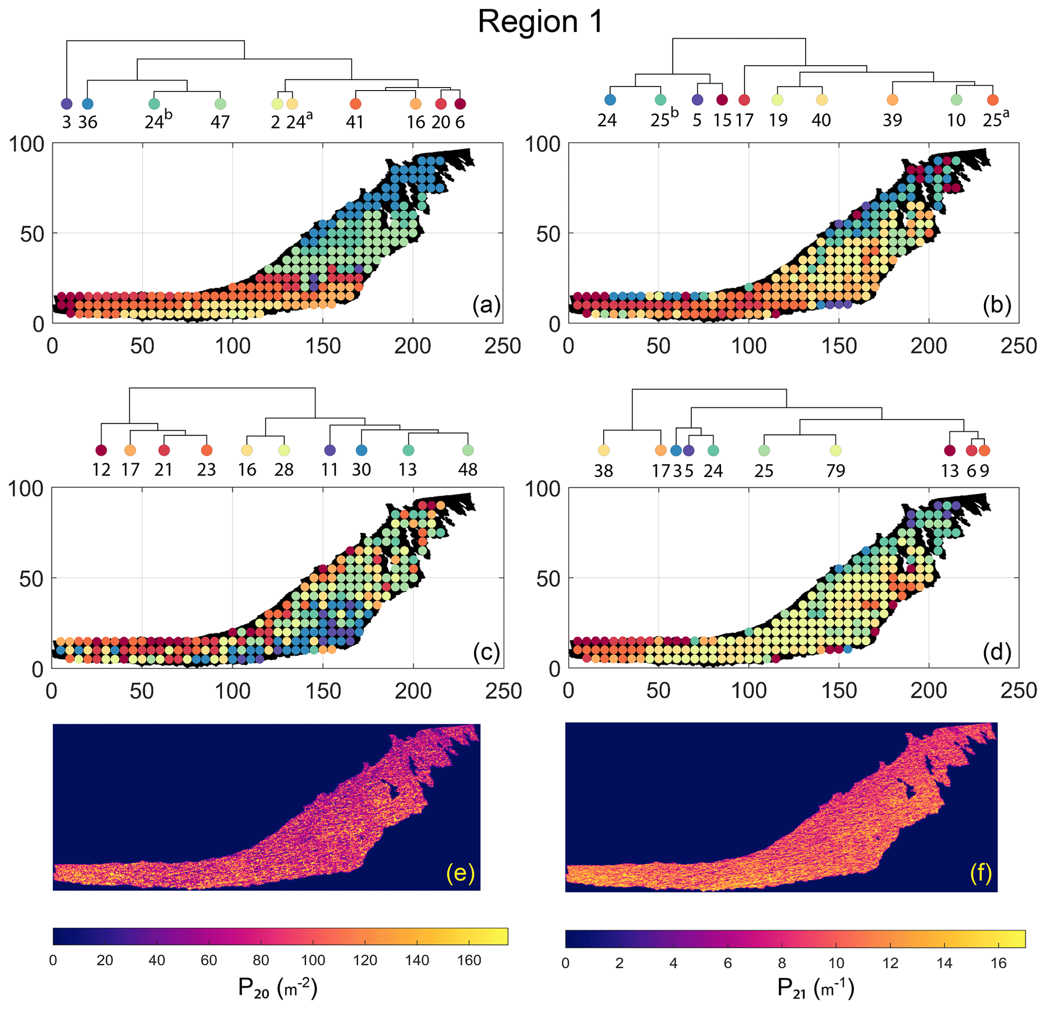
Figure 17 Hierarchical clustering results for Region 1 depicting the top 10 clusters using (a) fingerprint distance, (b) D-measure distance, (c) NetLSD distance, (d) portrait divergence distance, (e) spatial P₂₀, and (f) spatial P₂₁.

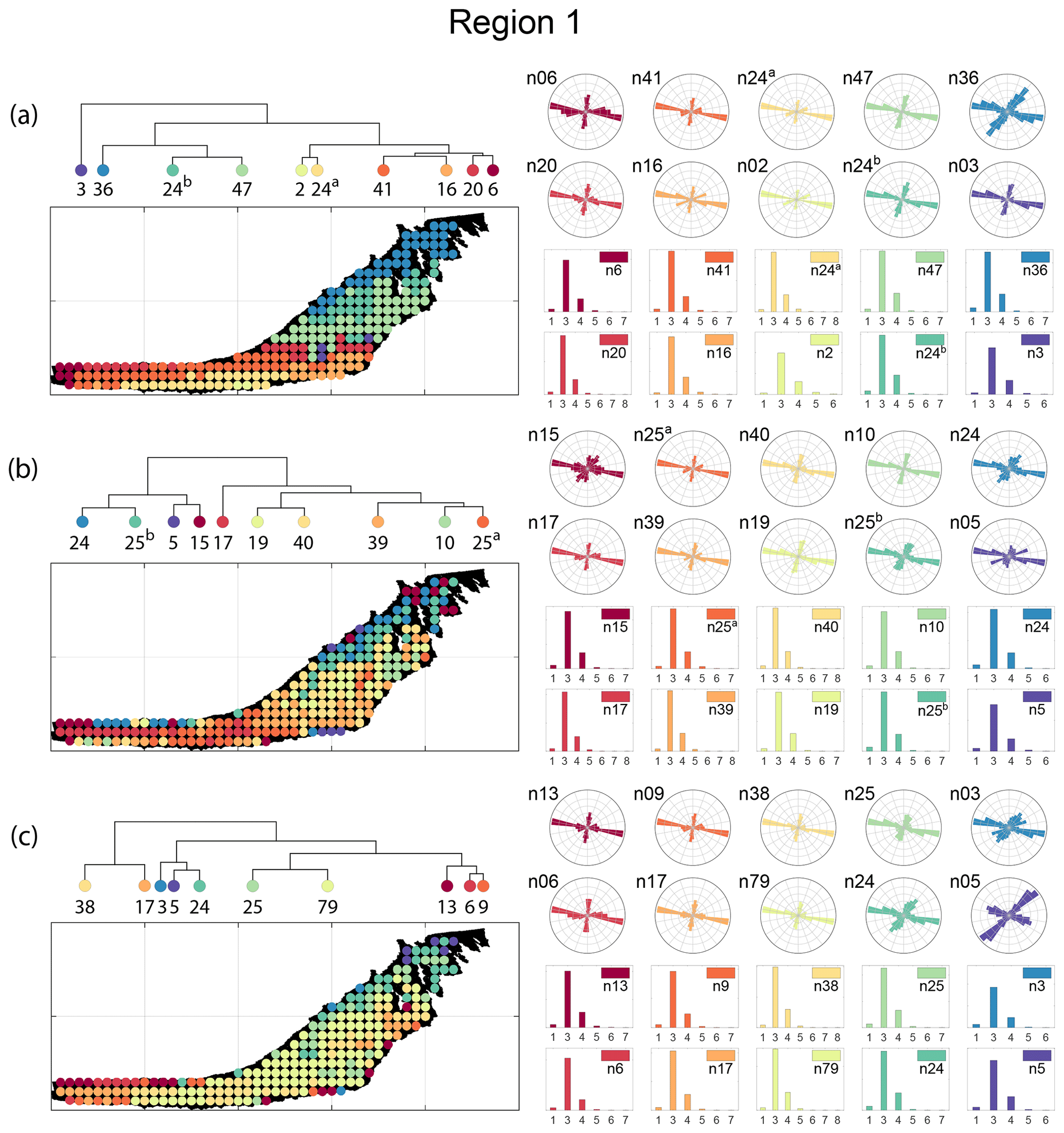
Figure 18 Variation in fracture orientations and topological summary for Region 1 corresponding to (a) fingerprint distance, (b) D-measure, and (c) portrait divergence.

5.2.2 Analysis of spatial variation in Region 2

Spatial distribution along with dendrograms of top 10 clusters pertaining to the four graph similarity measures for Region 2 is depicted in Fig. 19. The full dendrograms and heatmaps are placed in Fig. A2 in the Appendix. The variation of spatial clusters with different choices of dendrogram cut heights is shown in Figs. B5–B8 in the Appendix. The number of subsamples for the four similarity measures pertaining to a dendrogram cut of k=10 is tabulated in Table 5. Similar to Region 1, there is marked spatial autocorrelation with FP (Fig. 19a), DM (Fig. 19b), and PD (Fig. 19d), whereas the LSD (Fig. 19c) shows a speckled pattern. The spatial clustering results can be compared with the fracture persistence plots in Fig. 19e and f.

Table 5 Summary of subgraphs within each cluster of Region 2 for k=10.

Node degree histograms and rose plots depict the differences in network topology and fracture orientations between the identified clusters pertaining to FP (Fig. 20a), DM (Fig. 20b), and PD (Fig. 20c). For all three measures, the shape of rose plots indicates a transition of principal orientations smoothly across clusters. For example, in Fig. 20a for FP, the more complex fracturing in the west of Region 2 is depicted by cluster n20 with a very diffuse rose plot, changing orientations to a predominantly orthogonal pattern in cluster n03. The DM (clusters n16 and n10 in Fig. 20b) and PD (clusters n08 and n17^b in Fig. 20c) also identify this region of orthogonal fracturing. The corresponding topological summaries also depict an increased proportion of degree-4 nodes as compared to the histograms of other clusters.

From FP clustering results (see Fig. 19a), the dendrogram identifies a western branch with clusters n20 and n22. The branch comprising of clusters n8, n3, and n4 correspond to the radial fracturing region identified by Gillespie et al. (1993) that originates from the fault in the SE of Region 2. Clusters n9, n17, and n36 all under a branch covering parts of Region 2 further away from the radial fracturing region. Clusters n41 and n52 originate under a branch forming the northern and eastern boundaries of Region 2. Figure C4 depicts archetypal subgraphs under each cluster in detail for FP. The clustering results of DM (Fig. 19b) and PD (Fig. 19d) appear to be similar and with dendrograms roughly splitting into three main branches that correspond to specific portions of Region 1. First is the radial fracturing area represented by branch-forming clusters n10, n16, and n23^b for D-measure (Fig. 19b) and branch-forming clusters n17^b and n8 for the portrait divergence (Fig. 19d). The area to the NW periphery of Region 2, farthest away from the fault, is represented by branch-forming clusters n19, n20, n14, and n25 for DM and by branch-forming clusters n24^a, n15^a, and n34 for PD. The transition region branch is represented within the DM dendrogram by clusters n38, n23^a, and n24 and within the PD dendrogram by clusters n24^b, n15^b, and n28. Figures C5 and C6 depict detailed subgraph examples for DM and PD, respectively.

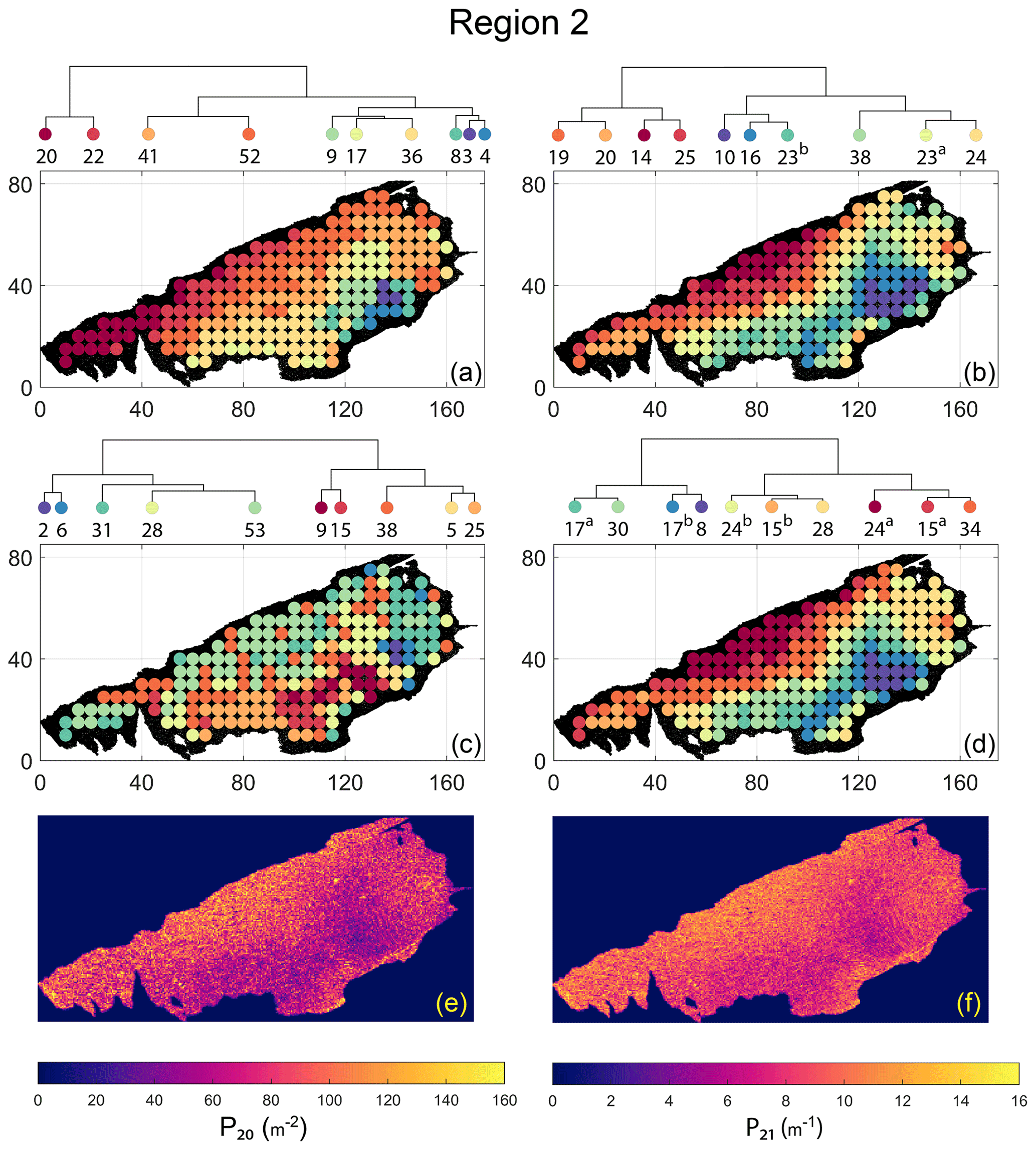
Figure 19 Hierarchical clustering results for Region 2 depicting the top 10 clusters using (a) fingerprint distance, (b) D-measure distance, (c) NetLSD distance, (d) portrait divergence distance, (e) spatial P₂₀, and (f) spatial P₂₁.

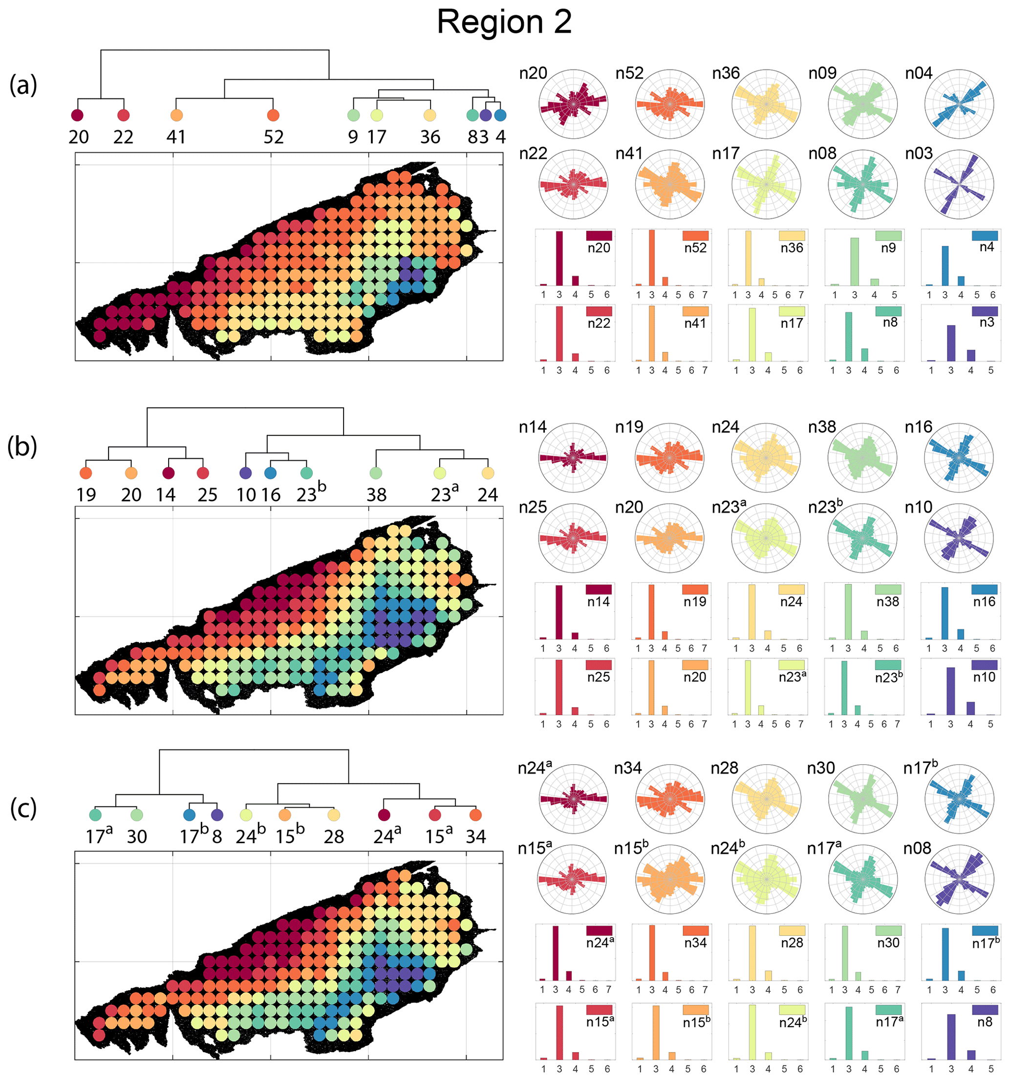
Figure 20 Variation in fracture orientations and topological summary for Region 2 corresponding to (a) fingerprint distance, (b) D-measure, and (c) portrait divergence.

5.2.3 Analysis of spatial variation in Region 3

The spatial distribution along with dendrograms of the top 10 clusters pertaining to the four graph similarity measures for Region 3 is depicted in Fig. 21. The full dendrograms and heatmaps are placed in Fig. A3 in the Appendix. The variation of spatial clusters with different choices of dendrogram cut heights (and number of clusters) is shown in Figs. B9–B12 in the Appendix. Similar to the Region 1 and 2 results, there is marked spatial autocorrelation with FP (Fig. 21a), DM (Fig. 21b), and PD (Fig. 21d), whereas the LSD (Fig. 21c) shows a stippled pattern. The spatial clustering results can be compared with the fracture persistence plots in Fig. 21e and f. The number of subsamples for the four similarity measures associated with a dendrogram cut of k=10 is tabulated in Table 6.

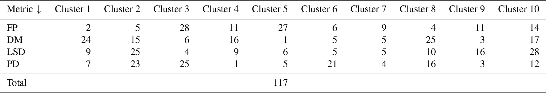
Table 6 Summary of subgraphs within each cluster of Region 3 for k=10.

Node degree histograms and rose plots depict the differences in network topology and fracture orientations between the identified clusters relating to FP (Fig. 22a), DM (Fig. 22b), and PD (Fig. 22c). For all three measures, the shape of rose plots indicates a transition of principal orientations smoothly across clusters. For example, in Fig. 22a for the fingerprint measure, the cluster n06 in the west of Region 3 has three main sets that become orthogonal in cluster n09, the nearest cluster eastwards. Cluster n05 at the eastern extremity of Region 3 has an orthogonal pattern that has rotated almost 80^∘ clockwise compared to the western boundary. Orientations of fractures clusters between the eastern-most and western-most clusters show transitions between the extremal archetypes.

From the FP clustering results (Fig. 21a), the spatial variation appears to have an E–W trend. From the dendrogram, an eastern branch comprising clusters n6, n9, n4, n11^a, and n14 and a western branch consisting of clusters n5, n28, n11^b, and n27 can be identified. An outlier branch with cluster n2 appears at the interface between the eastern and western branches. Detailed visualization of archetypal subgraphs relating to each of the FP clusters is presented in Fig. C7. The dendrogram structure and spatial clustering for the DM (Fig. 21b) depicts a central region represented by a branch containing clusters n24, n15, n6, and n16. The eastern and western peripheries organize as clusters n1, n5^a, n5^b, n25, n3, and n17 under a second branch. Underneath this branch, clusters n1, n5^a, and n5^b correspond to extremities of the Region 3, which are not fully sampled. The dendrogram structure for the PD (Fig. 21d) is similar with clusters n7, n23, n25 organizing under the branch representing the central region and clusters n1, n5, n21, n4, n16, n3, and n12 forming the eastern and western peripheral regions. Clusters n1 and n5 pertain to extremities of Region 3, which are not fully sampled. Figures C8 and C9 depict zoomed-in sections of the subgraphs relating to each of the top clusters that confirm the detected intra-regional variation for DM and PD, respectively.

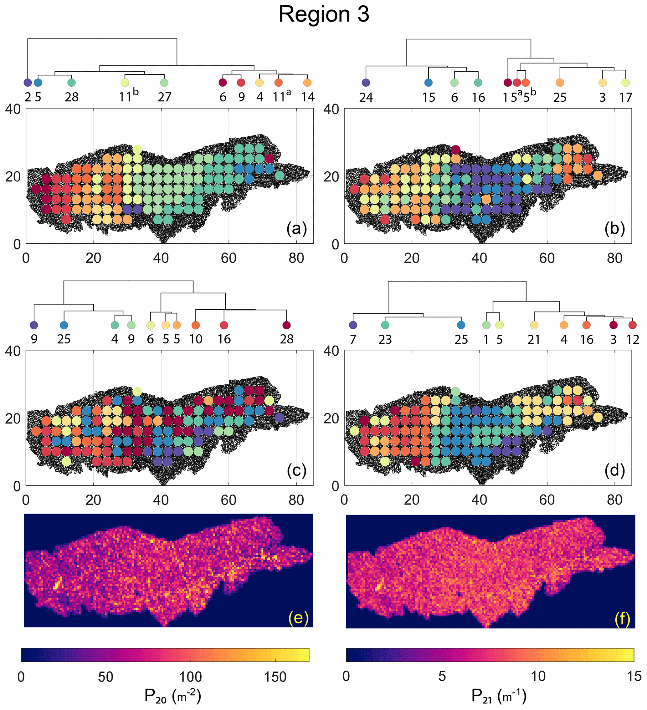
Figure 21 Hierarchical clustering results for Region 3 depicting the top 10 clusters using (a) fingerprint distance, (b) D-measure distance, (c) NetLSD distance, (d) portrait divergence distance, (e) spatial P₂₀, and (f) spatial P₂₁.

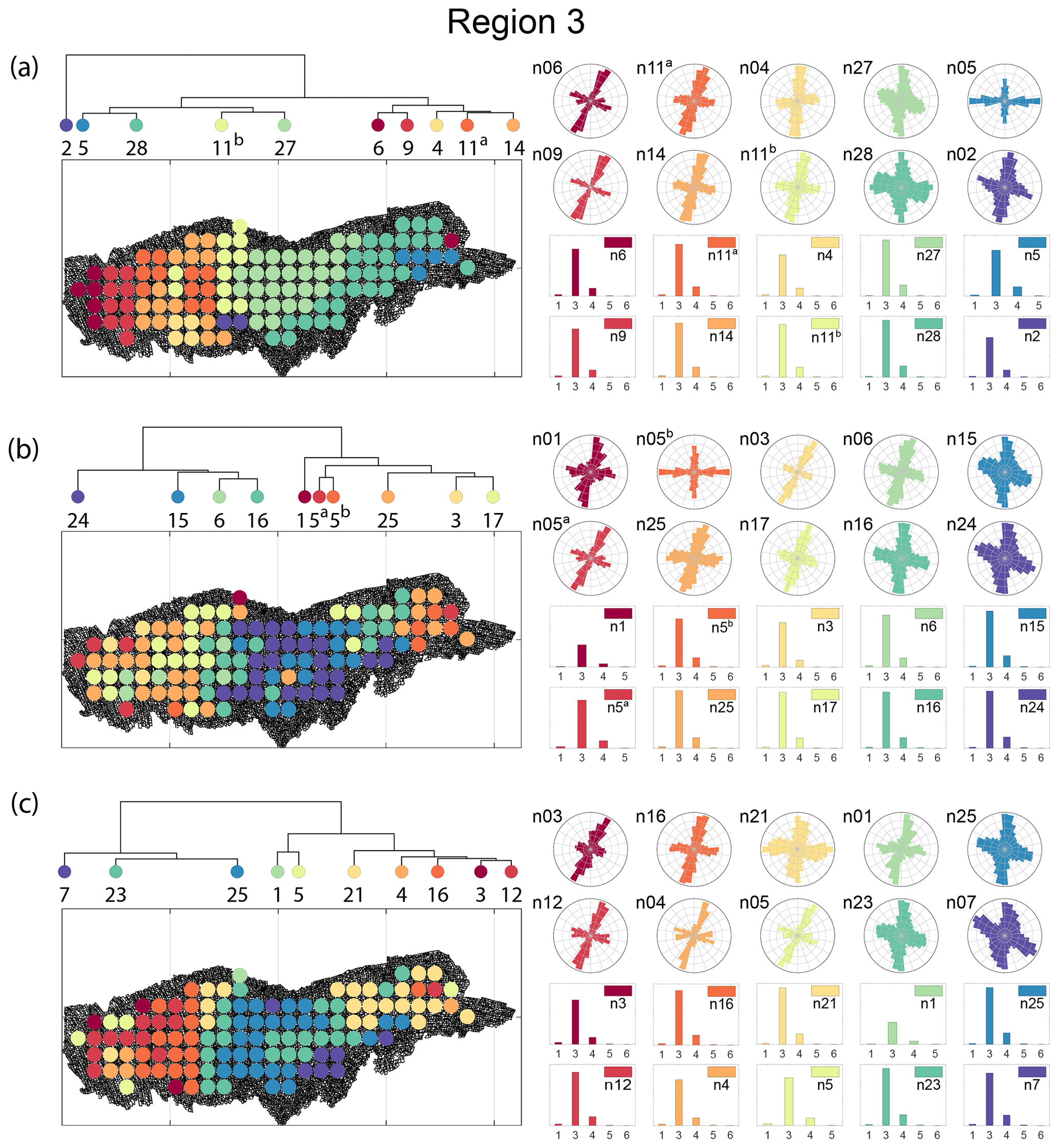
Figure 22 Variation in fracture orientations and topological summary for Region 3 corresponding to (a) fingerprint distance, (b) D-measure, and (c) portrait divergence.

6 Discussion

Within the structural geology literature, the quantitative fracture persistence measures of Dershowitz and Herda (1992), the topological approach of Sanderson and Nixon (2015), and qualitative descriptions are most commonly resorted to for comparing 2-D fracture networks. The lack of quantitative measures for spatial network data is partially due to the lack of extensive 2-D fracture trace data. Using the fully mapped, UAV-derived dataset of an extensive fracture network, it is possible to systematically investigate 2-D fracture network organization variations.

In this contribution, we treat 2-D fracture networks as planar graph structures and apply graph similarity measures to quantitatively compare subsampling within large fracture networks and discover clusters of similarity. The statistical technique of HC was used along with graph distance metrics to extract spatial clusters. Subgraphs within a spatial cluster are more similar to each other than other clusters. A hierarchy of patterns is derived based on similarity scores, which can be examined at deeper levels.

One can argue that variation exists at multiple length scales, and more granular inquiry would lead to different clusters. While our choices of grid spacing and subsampling of graphs were to keep computational requirements in mind, it is possible to do more dense subsampling than what we have already achieved to further highlight spatial variations within a given network. The clusters that we have depicted are particular to the spacing and sampling diameters that we have chosen. In this section, we discuss some additional perspectives and issues related to our methodology and results.

• Linking spatial variation patterns to fracturing drivers. The results indicate that spatial variation in fracture networks is not always evident from the ubiquitously used fracture persistence measures, such as P₂₀ and P₂₁. The proposed method highlights variations in network structure which can then help draw inferences into possible drivers for the spatial differences. In the case of Regions 2 and 3, the proximity to the fault influences network development. Such a model has been proposed by Peacock and Sanderson (1995); Gillespie et al. (2011) and Wyller (2019), where the oldest fractures are long and radial, emanating from local asperities within the fault. These older fractures then influence the development of younger fractures. This is observed in Region 2, where clusters form roughly parallel to the E–NE-striking fault with the direction of variation to the NW. Region 3 is positioned between two such asperity epicentres. There are long, radial fractures on the eastern and western extremities with a transition region in between. The direction of cluster variation trends E–W. Fracture pattern variation in Region 1 is not affected by faulting. Since Regions 1 and 2 pertain to a single layer, the NE regions of Region 1 show visual similarities between the westernmost extremities of Region 2. The intra-regional variations in Region 1 could be due to layer thickness variation, although we do not have sufficient thickness data to confirm this.

  The analysis of spatial variation can assist in deciphering fracture timing. Given the temporal nature of network formation, it is desirable to delineate network evolution into relative episodes of fracturing. In previous analyses specific to the Lilstock dataset used in this contribution, Passchier et al. (2021) identified jointing sets with timing history based on fracture length, strike, and topological relationships. Although the temporal history is identified from joints that were picked manually but not wholly by Passchier et al. (2021), there is still a discernable spatial variation where some jointing sets are localized while others occur throughout the outcrop. Identifying spatial clustering in complete networks provides a basis by which joint sets can then be arranged in a hierarchy of temporal development.

• On the choice of a graph distance metric. We have restricted our investigation scope to four state-of-the-art graph similarity distances from the recent graph theory literature. Many more graph distances applicable to spatial graphs exist (Hartle et al., 2020; Tantardini et al., 2019); furthermore, the best means remain an open problem in network science research. Some novel distance measures are not graph based but derive from persistent homology (such as Feng, 2020). In this approach that considers the shape of data, persistence diagrams are generated from spatial graphs, and bottleneck distances are combined with hierarchical clustering to discover clusters. The results from Feng (2020) compared favourably to that of Louf and Barthelemy (2014) when applied to patterns of cities.

  As may be observed from our results, the metrics highlight certain aspects of the fracture network while not considering others. For instance, the fingerprint distance only considers block area and shape factor distributions of the blocks and neglects orientations. The other three distances use graph properties directly, and hence orientation information (or the lack of it) is a consequence of how the spatial graph is defined. We used weighted graphs that incorporate Euclidean distance between nodes as edge weights for the similarity computations. However, each edge also has a striking attribute to completely describe its position in 2-D space (in the case of 3-D, it needs a dip). Ideally, the edge weight should then be a vector, $w=[l,\mathit{\theta }]$ incorporating both lengths, “l” and orientation, “θ”, but the distance metrics we use do not allow the use of non-scalar weights.

• Do REVs exist for fracture networks? In the context of fractured reservoir modelling, identification of a REV aids continuum-based simulation approaches. However, the complexities of fluid flow and transport through fractured porous media require an explicit representation of fractures. Given the difficulties associated with obtaining realistic network geometries, stochastic-process-based methods derived from sparse fracture data are commonplace. However, these methods are often unable to represent inherent non-stationarity in spatial variation (Thovert et al., 2017), and work by Andresen et al. (2013) finds that discrete fracture networks (DFNs) from nature exhibit disassortativity, which is not a property of generated networks. Other techniques based on multipoint statistics (Bruna et al., 2019b) attempt image-based approaches to modelling non-stationary networks. Estrada and Sheerin (2017) present a different approach in which DFNs are directly generated as spatial graphs (referred to as “random rectangular graphs”). Such a method can incorporate insights from outcrop-derived naturally fractured reservoirs (NFRs).

  Regardless of the extrapolation method used, stationarity decisions have to be made based on hard data, and this is where our approach is helpful. We can use outcrop-derived networks to define and delineate stationarity's spatial boundaries and assign a particular type of network with due cognition of the inherent graph structure. Much literature exists on linking fracture patterns to high-deformation drivers such as folding, faulting, and diapirism, with the goal being to identify and correlate appropriate outcrop analogues to particular subsurface conditions. As our clustering results indicate, at the dimensional scales of sampling we have used, Tobler's first law of geography applies to fracture networks. Therefore, a representative network based on network similarity can be derived. The method can be applied to analogues for which data already exist. Further work is required to differentiate fluid-flow and transport responses of the identified cluster type.

• Other clustering methods. We have used a combination of HC and graph distance metrics to delineate regions within a spatial graph and arrange them in a hierarchy of similarities. Within the graph theory literature, there are other non-HC methods based on graph properties such as modularity (Newman and Girvan, 2004; Blondel et al., 2008; Traag et al., 2019) or by graph spectral partitioning (Fiedler, 1973; Spielman and Teng, 2007). Recent developments using graph neural networks and graph machine learning include modifications on the concept of modularity (Tsitsulin et al., 2020) and spectral methods (Bianchi et al., 2020) towards the goal of partitioning graphs into clusters.

7 Conclusions

This contribution presents a method to automatically identify spatial clusters and quantify intra-network spatial variation within 2-D fracture networks. We test the technique on 2-D trace data from a prominent limestone outcrop within the Lilstock pavements, located off the southern coast of the Bristol Channel, UK. The fracture network data that span three separate regions and cover over 14 200 m² are converted to the form of planar graph structures, spatially sampled into subgraphs, and then compared using four different graph-distance measures. The pair-wise similarities in the form of distance matrices are used to arrange region-wise subgraphs into a hierarchical relationship structure, also referred to as a dendrogram, using the statistical technique of hierarchical clustering. Positional order information from the dendrogram is used to render maps depicting the spatial variation within the fracture networks. The delineations of these intra-network subpatterns provide a way to identify representative elemental volumes that preserve fracture networks' topological and geometric properties. The presence of these subregions can also serve as a guide for making decisions on stationarity with respect to geostatistical modelling. The main findings of the study are summarized as follows:

• Representing fracture networks as graphs enables combining hierarchical clustering and graph-distance metrics to reveal interesting intra-network spatial similarity patterns not otherwise discernable from existing global or local fracture network descriptors.

• Organization of fracture network subgraphs based on pair-wise similarities into a hierarchical tree enables identification of spatial clustering at different dendrogram heights with newer and more granular cluster boundaries emerging at successively deeper levels of enquiry.

• Spatial autocorrelation is more apparent with the fingerprint, D-measure, and the portrait divergence distances than the NetLSD, which yields speckled patterns with little or no spatial autocorrelation.

• Spatial variation maps deriving from hierarchical clustering using the D-measure and portrait divergence identify similar spatial clusters and cluster boundaries. However, with the fingerprint distance, the cluster boundaries are different.

• Fracture segment orientations show gradual variation in segment strikes across the identified clusters despite orientation not being explicitly considered and only Euclidean distance being used to weight spatial graph edges.

Appendix A: Heatmaps and dendrograms

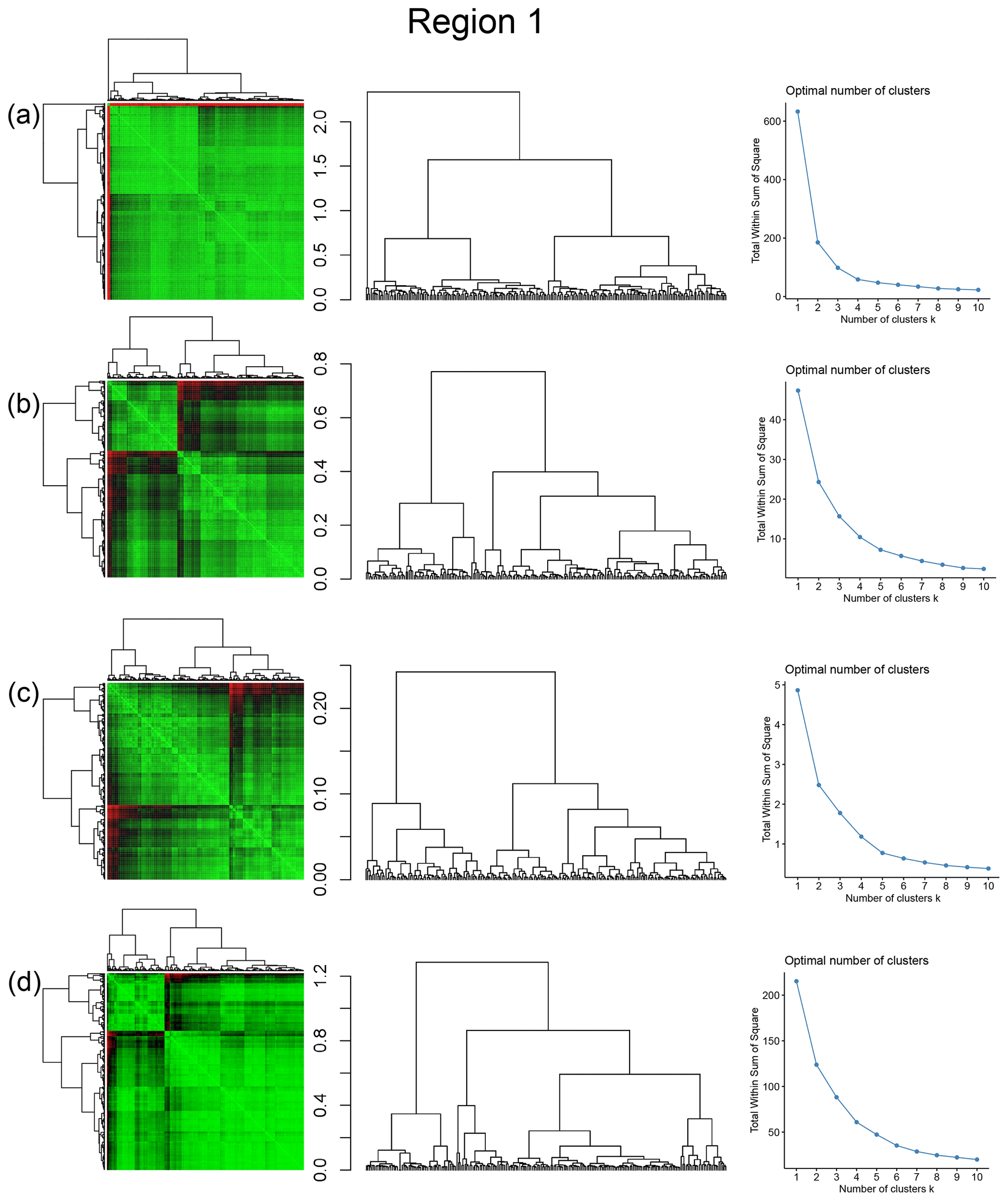
Figure A1 Combined symmetric heatmap of distance matrix and dendrograms, dendrograms, and sum-of-squares elbow plots for Region 1 (a) fingerprint distance, (b) D-measure, (c) NetLSD, and (d) portrait divergence.

Figure A2 Combined symmetric heatmap of distance matrix and dendrograms, dendrograms, and sum-of-squares elbow plots for Region 2 (a) fingerprint distance, (b) D-measure, (c) NetLSD, and (d) portrait divergence.

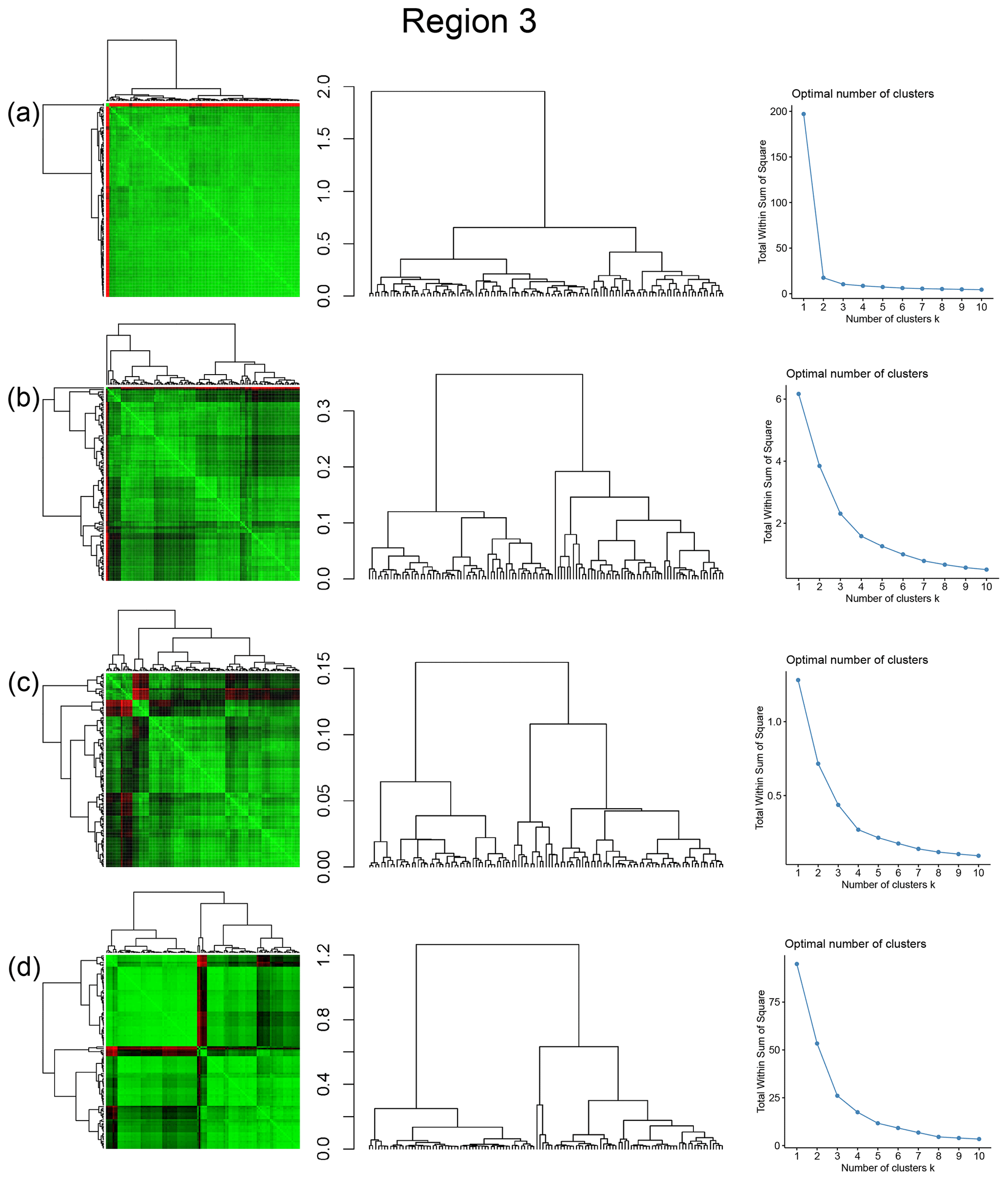
Figure A3 Combined symmetric heatmap of distance matrix and dendrograms, dendrograms, and sum-of-squares elbow plots for Region 3 (a) fingerprint distance, (b) D-measure, (c) NetLSD, and (d) portrait divergence.

Appendix B: Spatial variation for different levels of dendrogram cuts

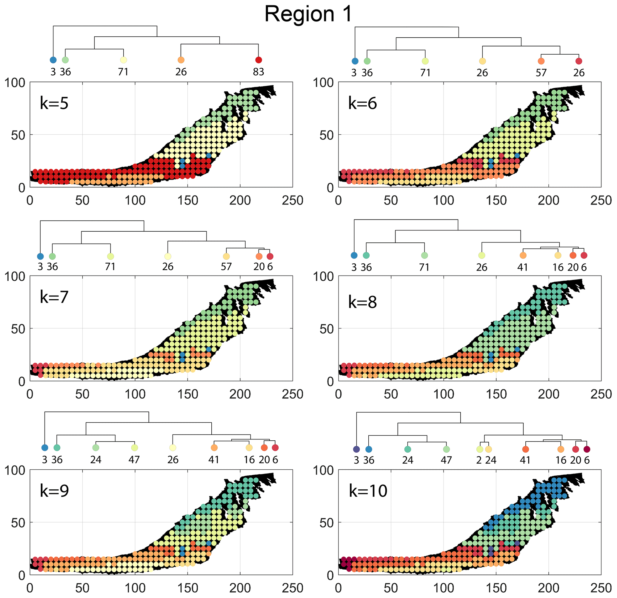
Figure B1 Variation in cluster boundaries for “k” clusters in Region 1 using fingerprint distance.

Figure B2 Variation in cluster boundaries for “k” clusters in Region 1 using D-measure.

Figure B3 Variation in cluster boundaries for “k” clusters in Region 1 using NetLSD.

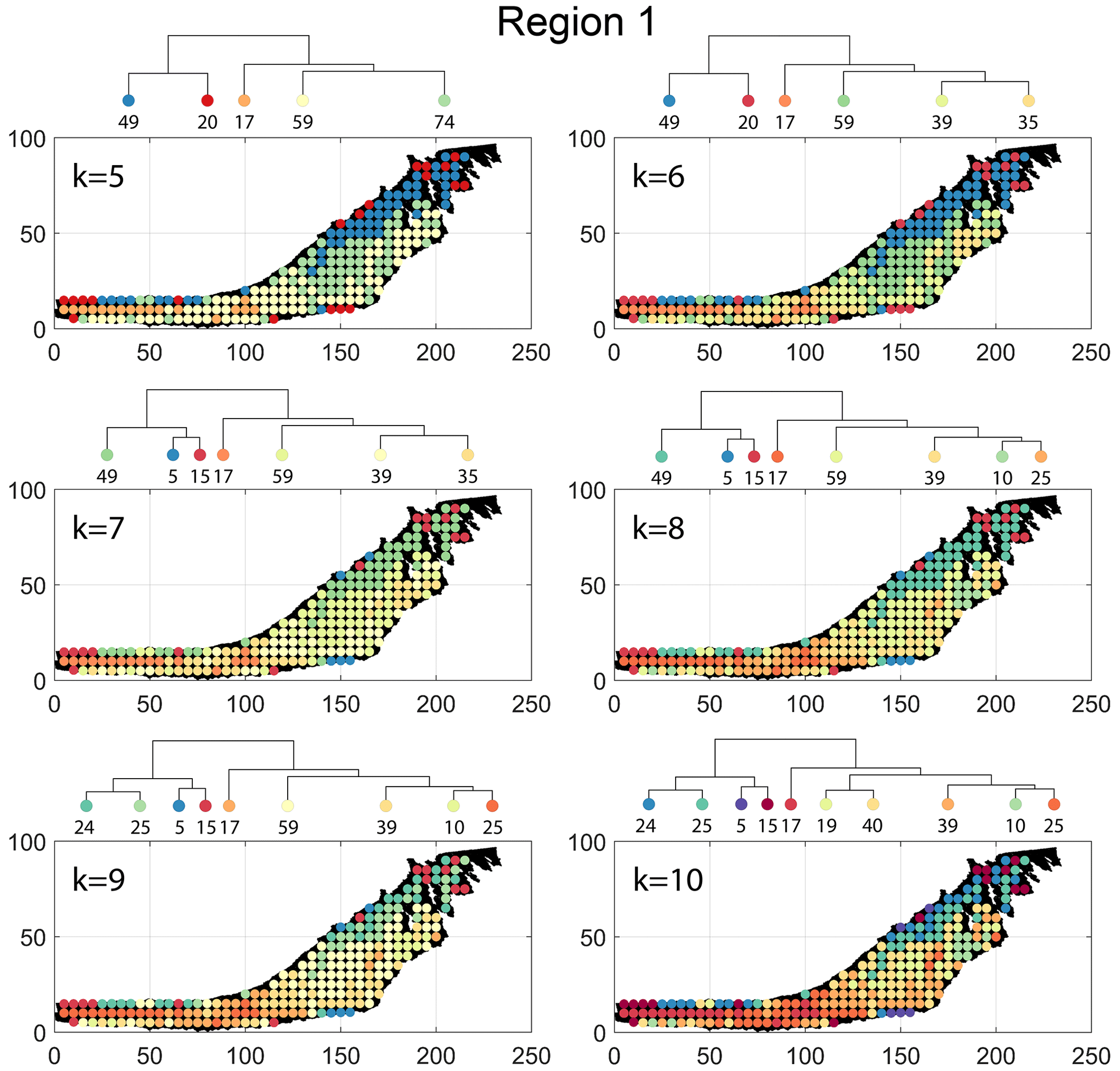
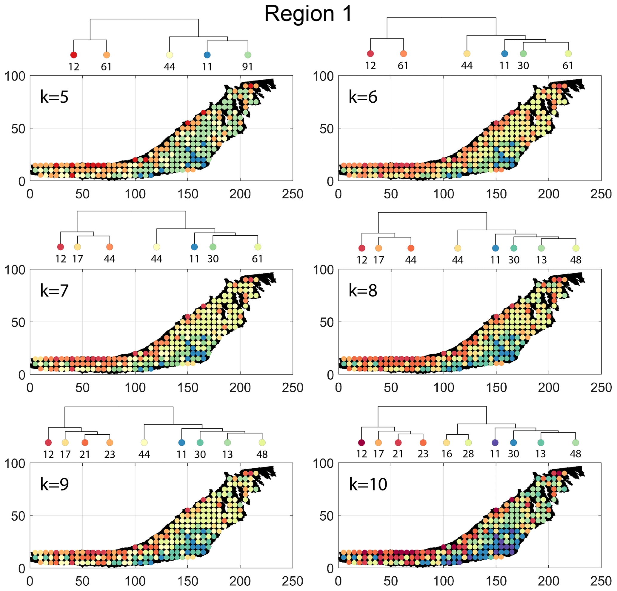
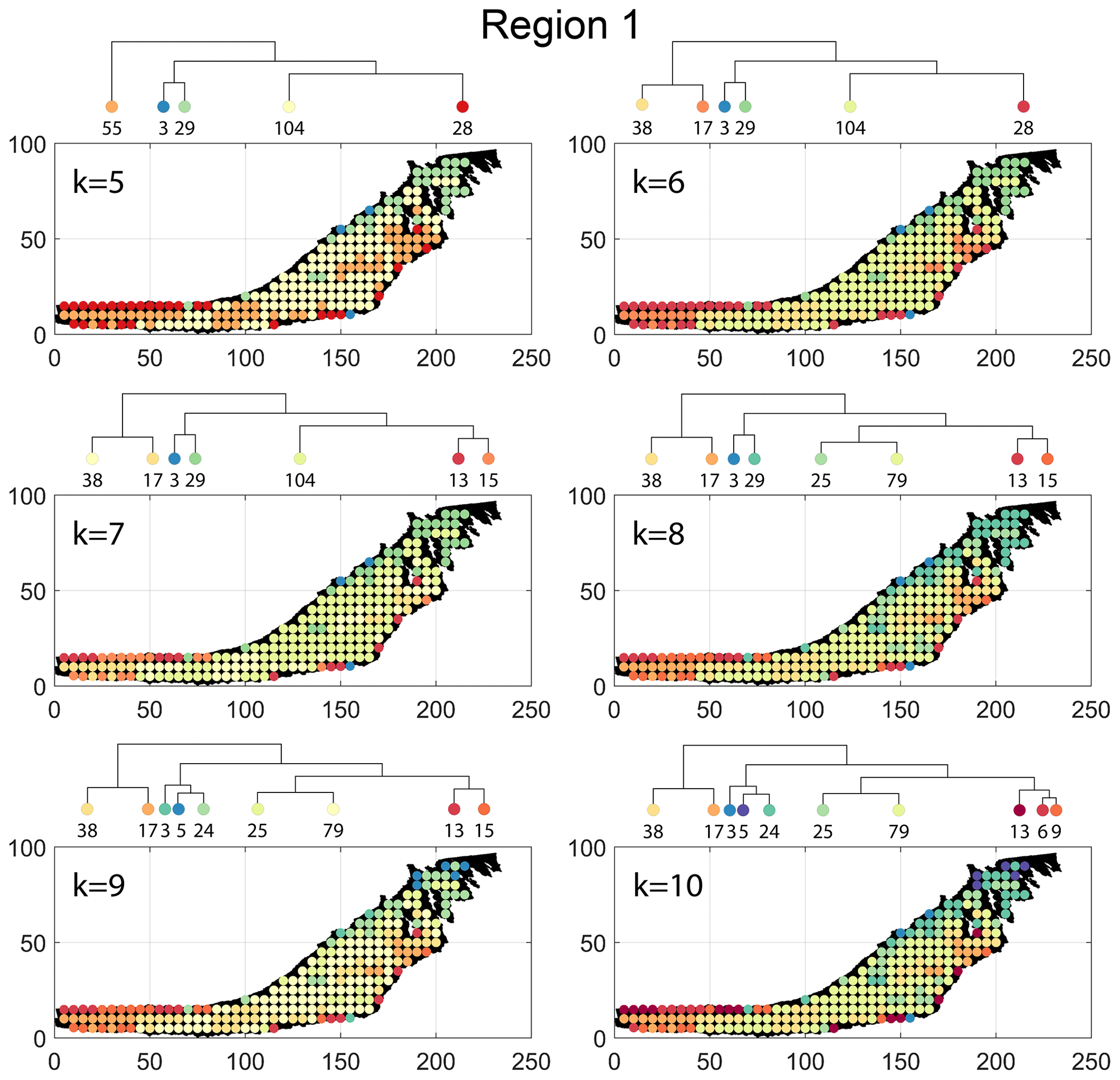
Figure B4 Variation in cluster boundaries for “k” clusters in Region 1 using portrait divergence.

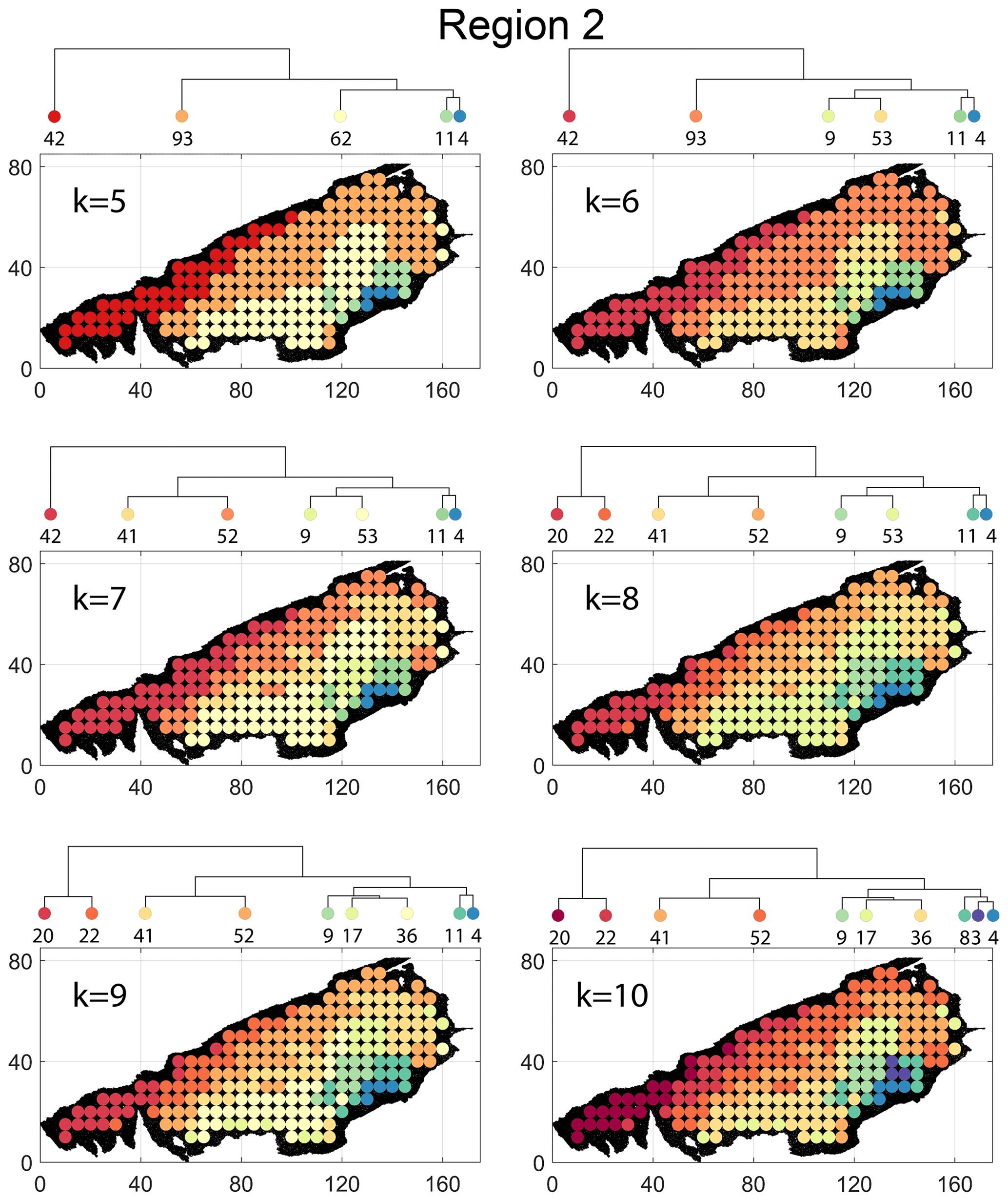
Figure B5 Variation in cluster boundaries for “k” clusters in Region 2 using fingerprint distance.

Figure B6 Variation in cluster boundaries for “k” clusters in Region 2 using D-measure.

Figure B7 Variation in cluster boundaries for “k” clusters in Region 2 using NetLSD.

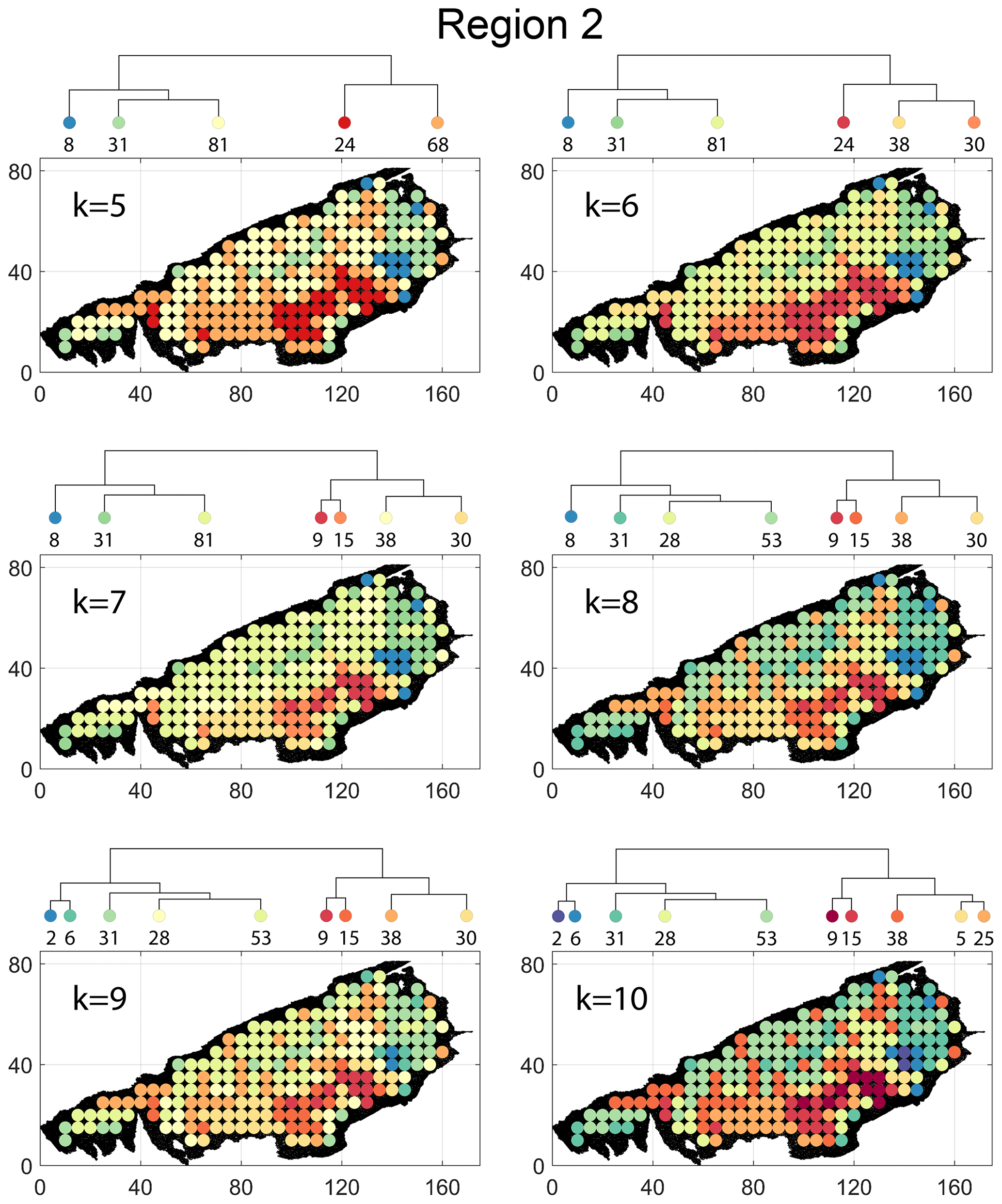
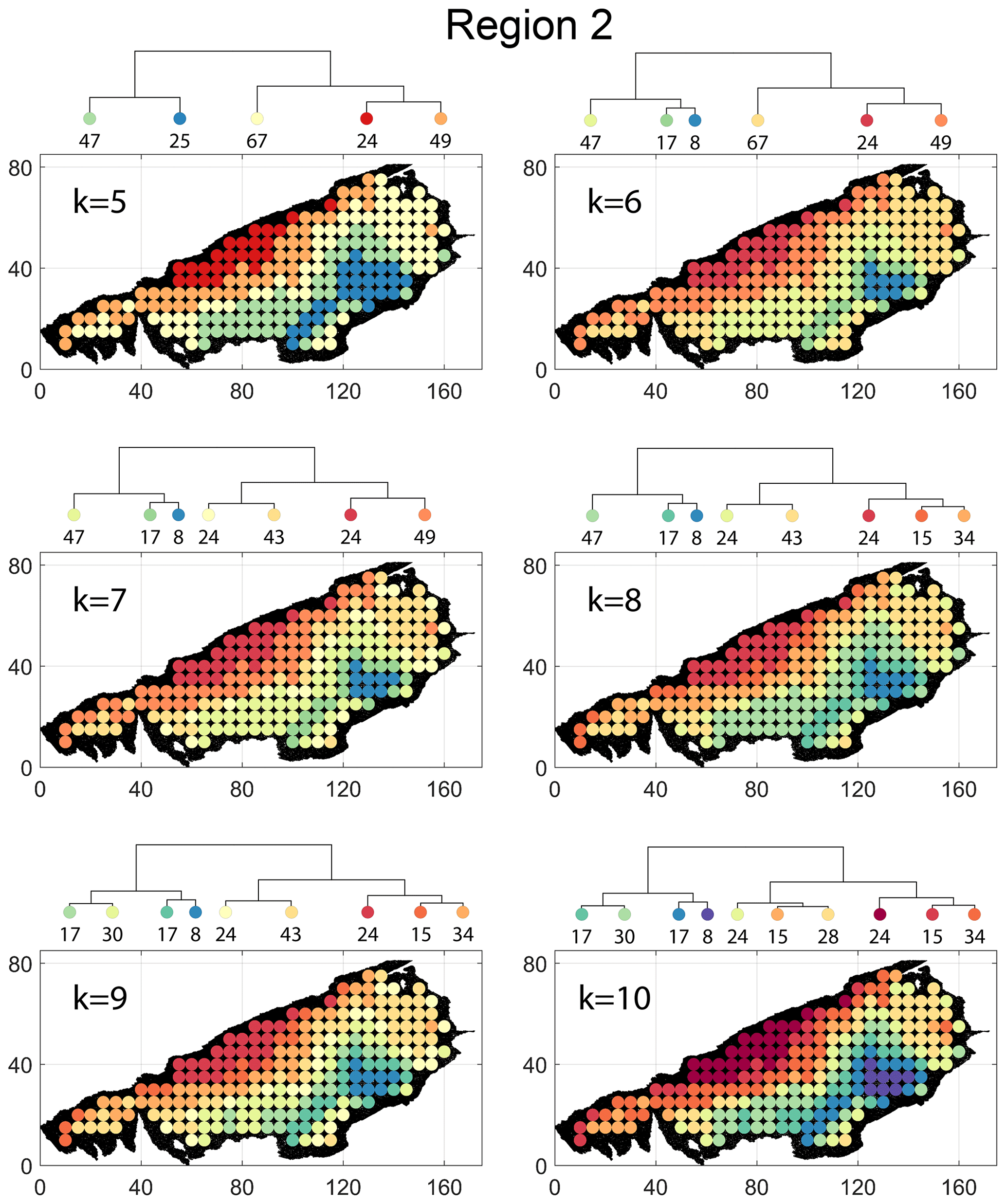
Figure B8 Variation in cluster boundaries for “k” clusters in Region 2 using portrait divergence.

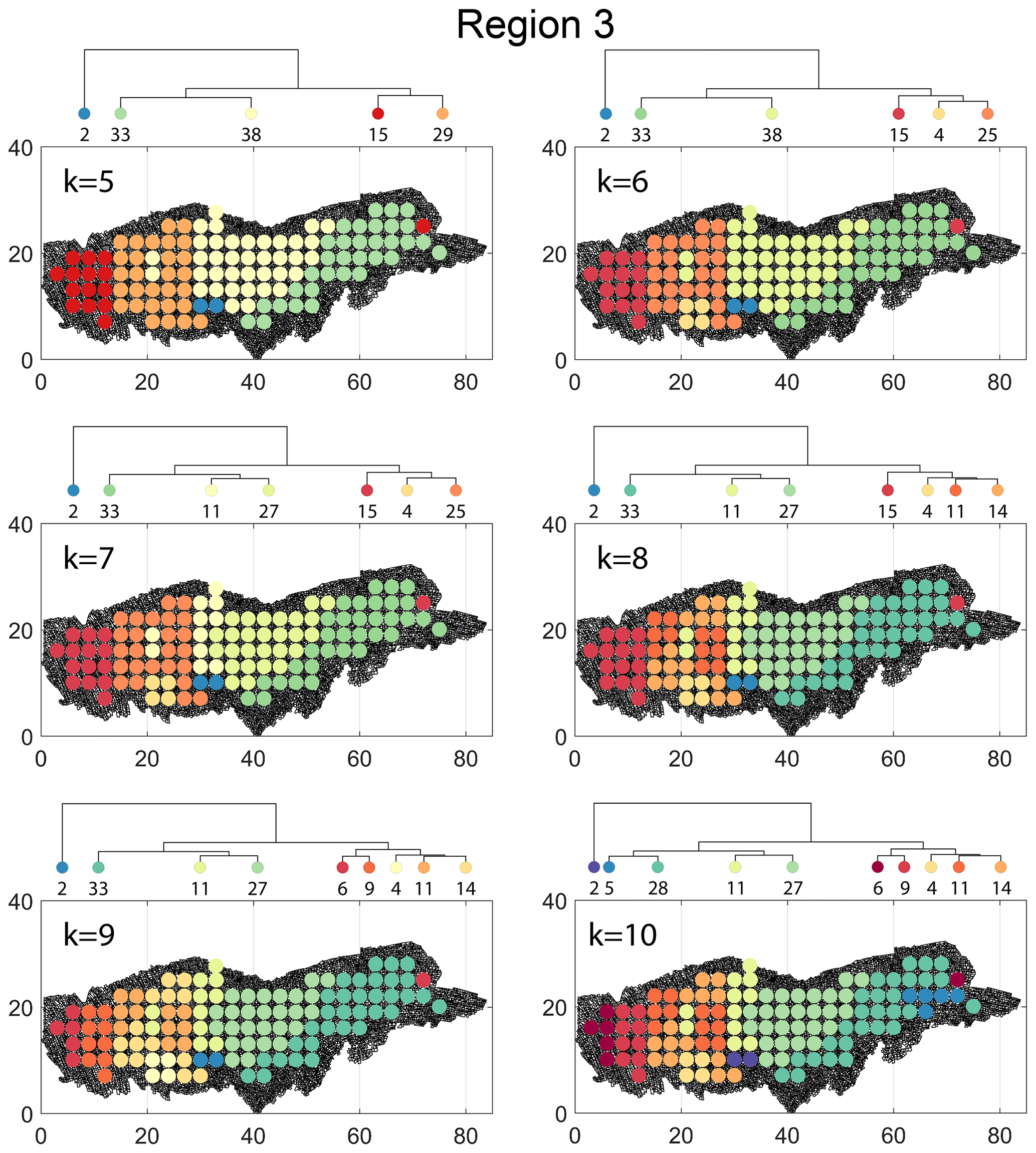
Figure B9 Variation in cluster boundaries for “k” clusters in Region 3 using fingerprint distance.

Figure B10 Variation in cluster boundaries for “k” clusters in Region 3 using D-measure.

Figure B11 Variation in cluster boundaries for “k” clusters in Region 3 using NetLSD.

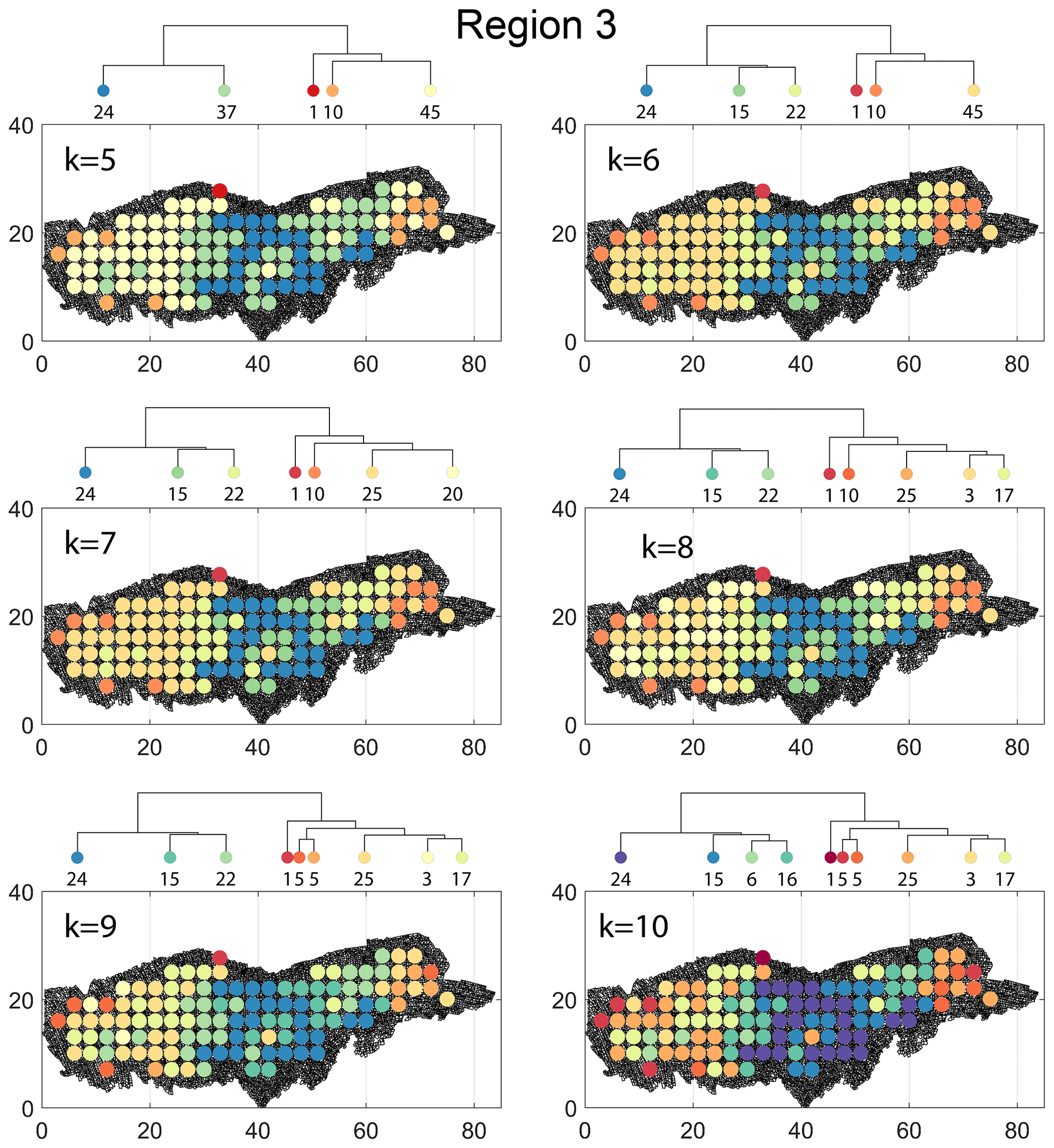
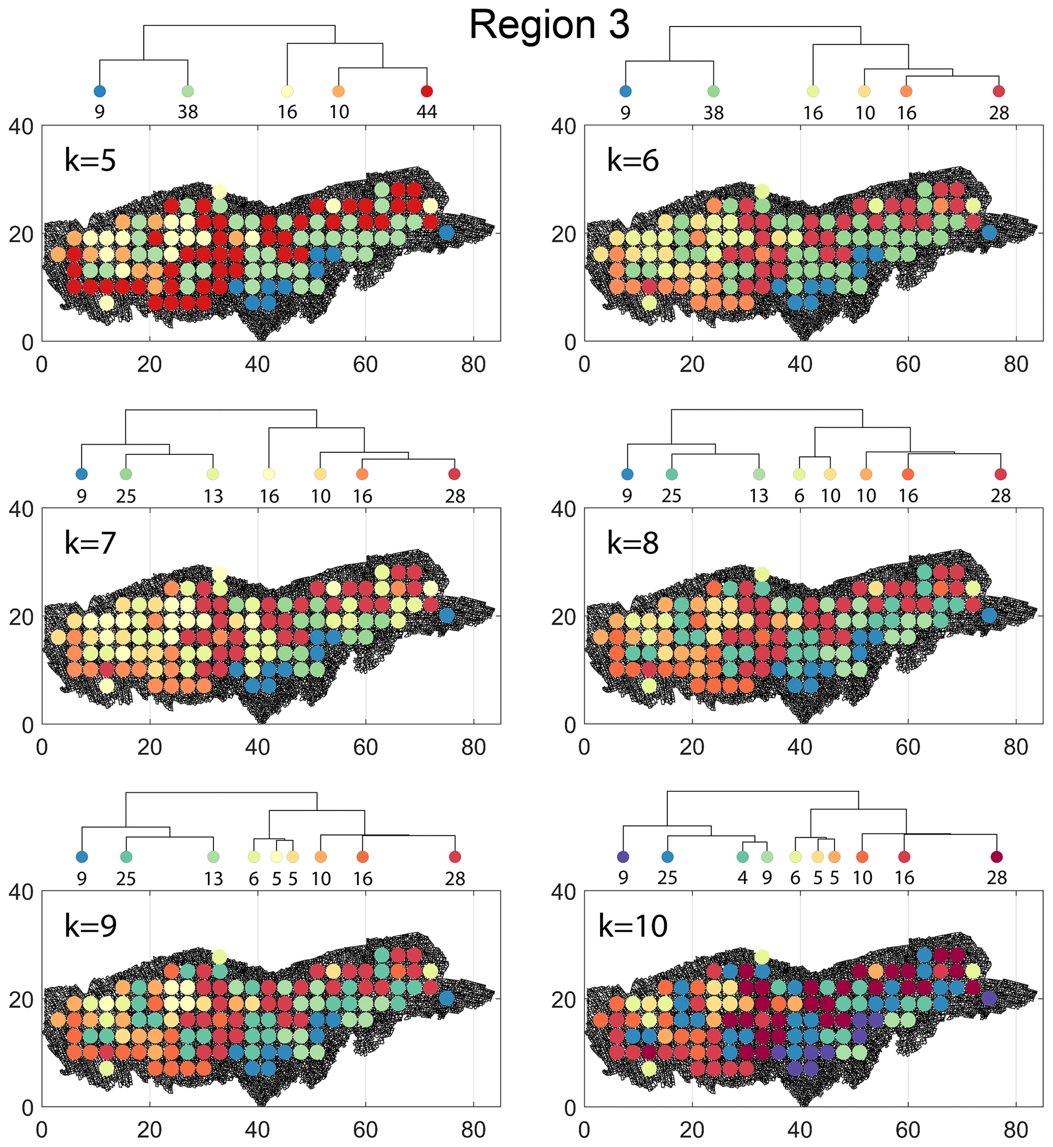
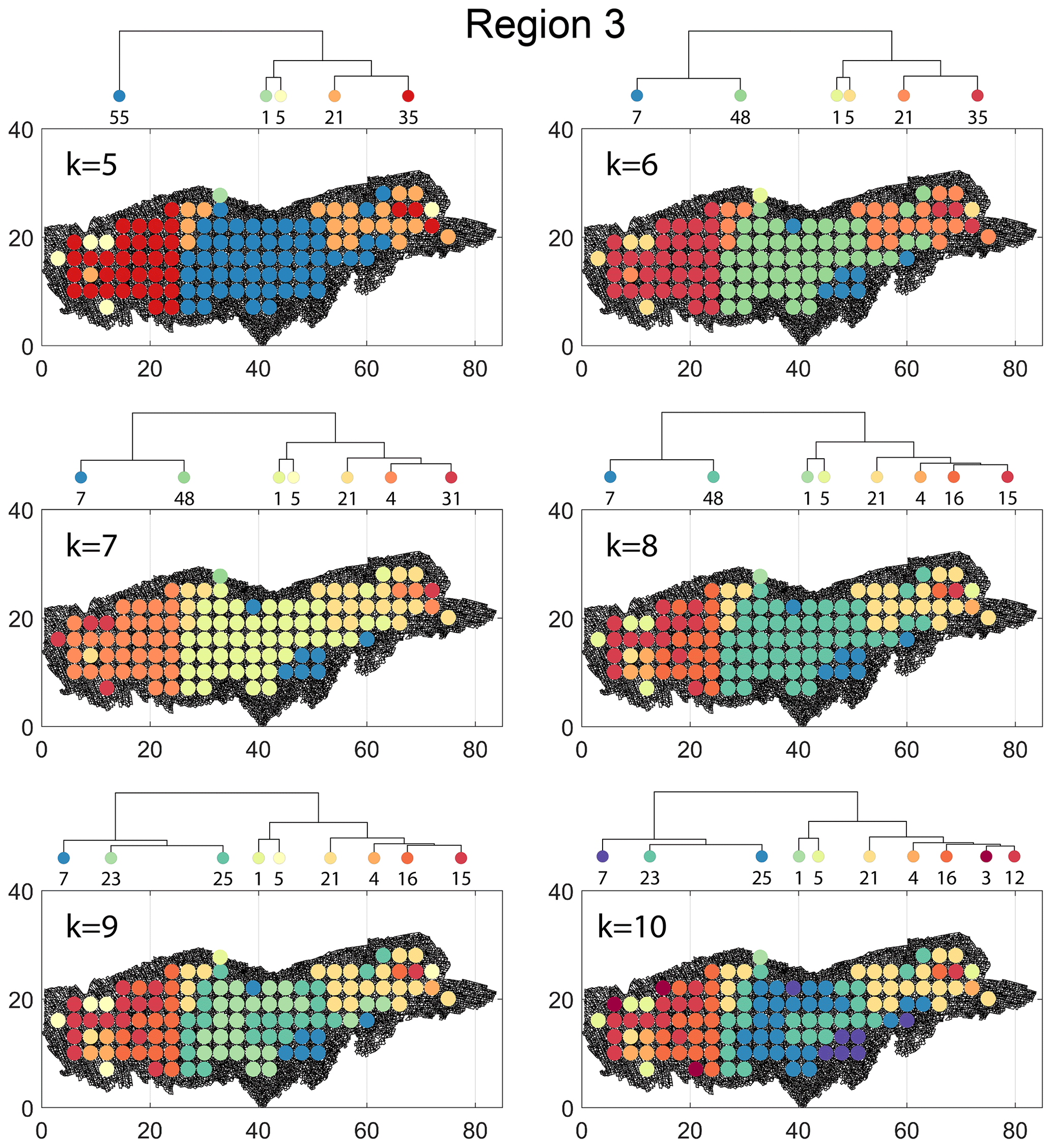
Figure B12 Variation in cluster boundaries for “k” clusters in Region 3 using portrait divergence.

Appendix C: Detailed spatial heterogeneity maps

Figure C1 Circular subgraph samples depicting variation in fracturing style as identified in the 10 largest clusters by fingerprint distance in Region 1. Coordinates of circular sample centres are below each subgraph example.

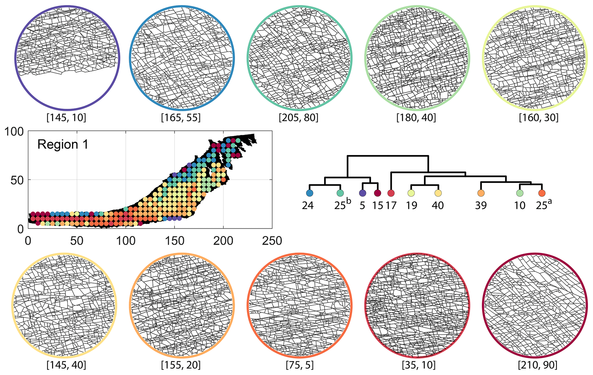
Figure C2 Circular subgraph samples depicting variation in fracturing style as identified in the 10 largest clusters by D-measure in Region 1. Coordinates of circular sample centres are below each subgraph example.

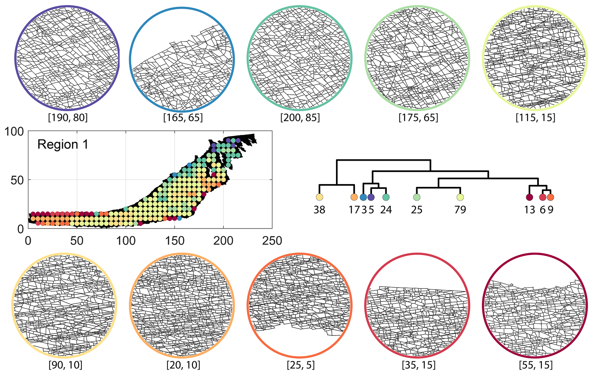
Figure C3 Circular subgraph samples depicting variation in fracturing style as identified in the 10 largest clusters by portrait divergence in Region 1. Coordinates of circular sample centres are below each subgraph example.

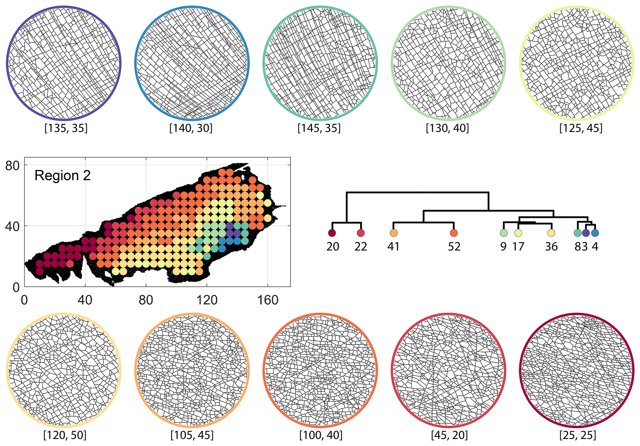
Figure C4 Circular subgraph samples depicting variation in fracturing style as identified in the 10 largest clusters by fingerprint distance in Region 2. Coordinates of circular sample centres are below each subgraph example.

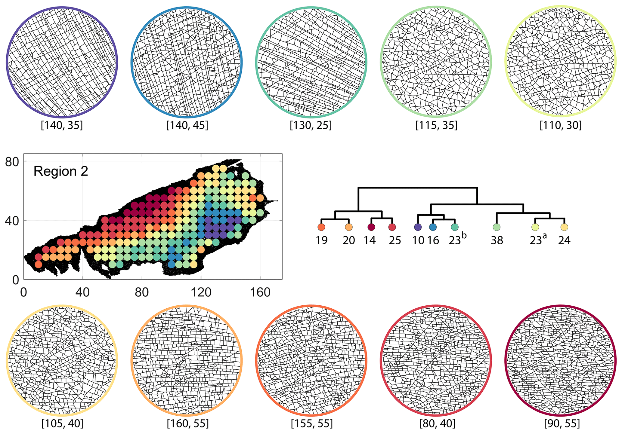
Figure C5 Circular subgraph samples depicting variation in fracturing style as identified in the 10 largest clusters by D-measure in Region 2. Coordinates of circular sample centres are below each subgraph example.

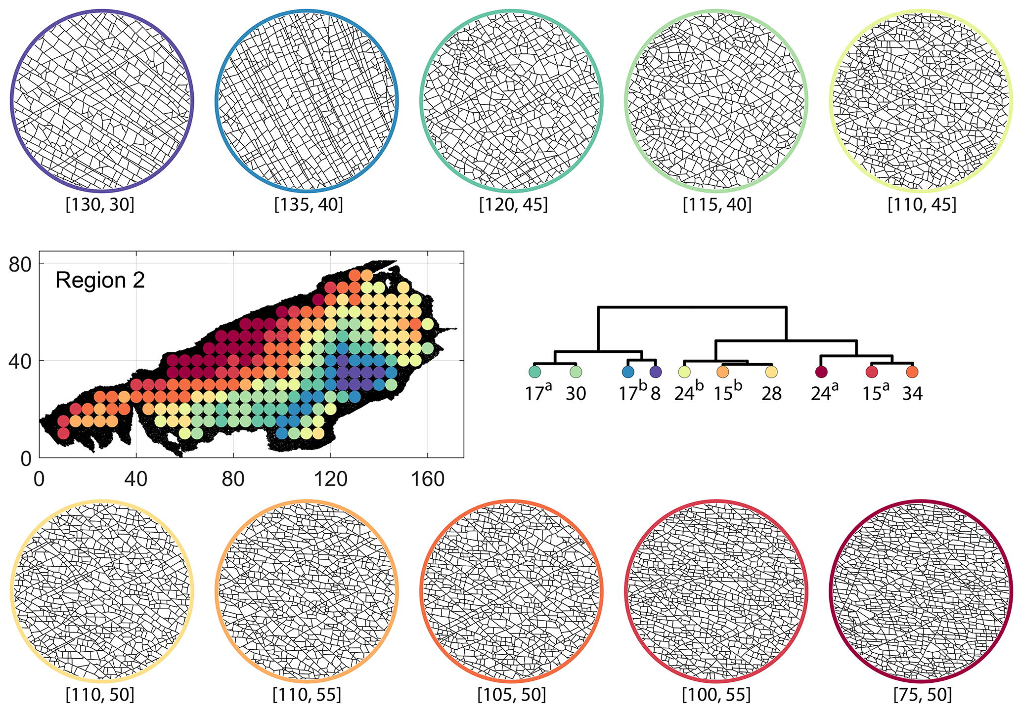
Figure C6 Circular subgraph samples depicting variation in fracturing style as identified in the 10 largest clusters by portrait divergence in Region 2. Coordinates of circular sample centres are below each subgraph example.

Figure C7 Circular subgraph samples depicting variation in fracturing style as identified in the 10 largest clusters by fingerprint distance in Region 3. Coordinates of circular sample centres are below each subgraph example.

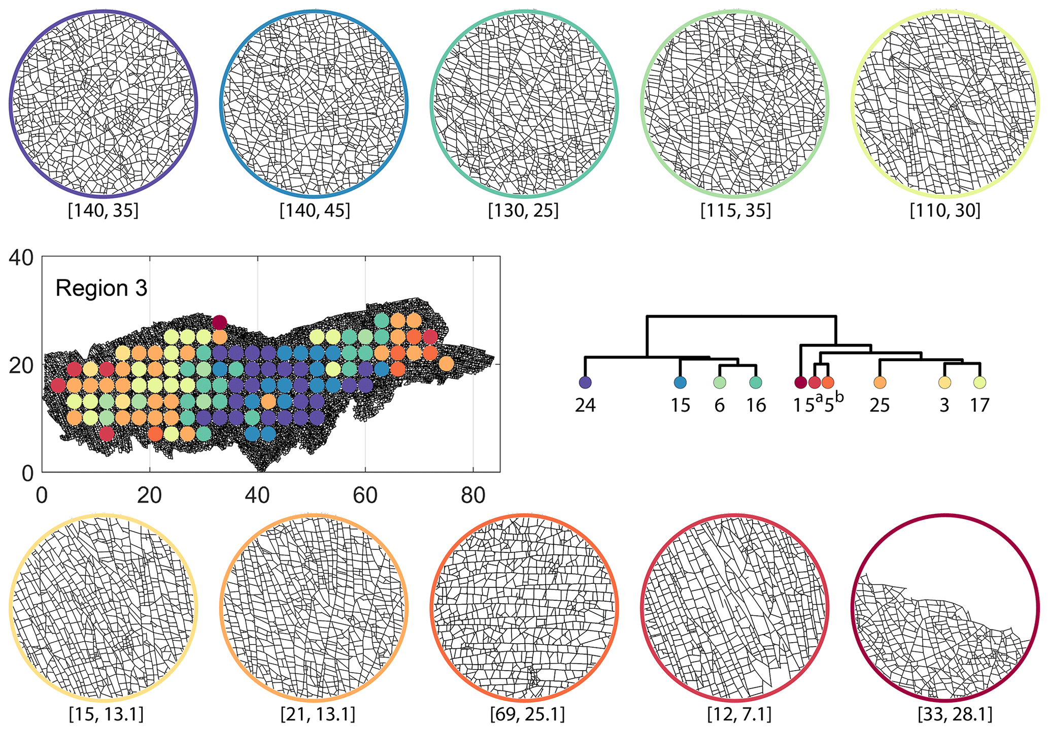
Figure C8 Circular subgraph samples depicting variation in fracturing style as identified in the 10 largest clusters by D-measure in Region 3. Coordinates of circular sample centres are below each subgraph example.

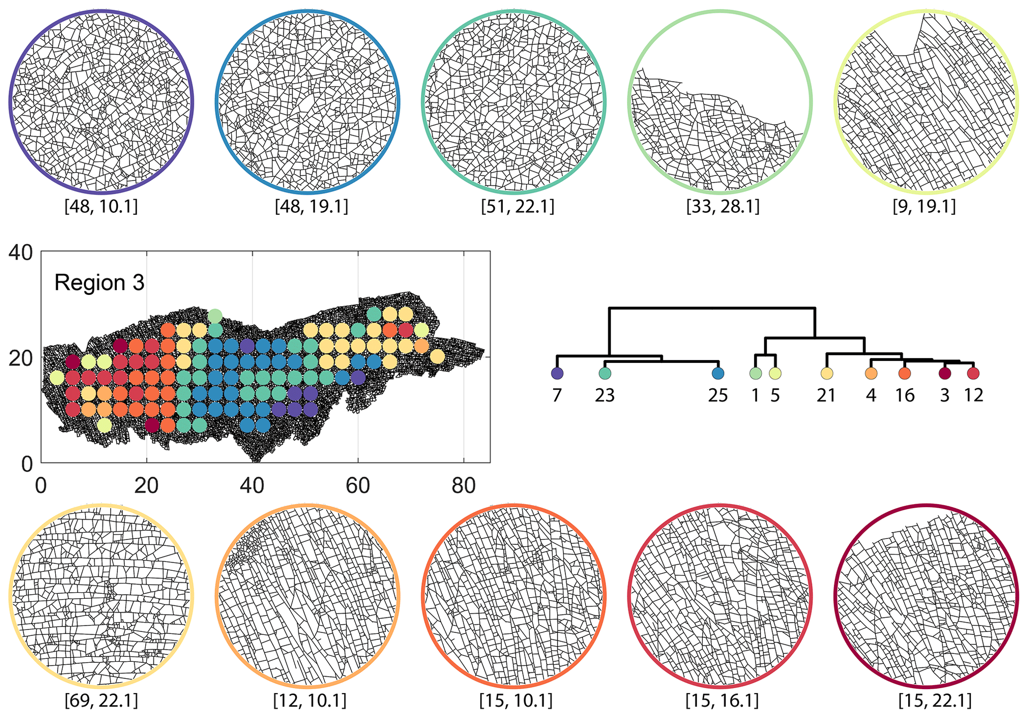
Figure C9 Circular subgraph samples depicting variation in fracturing style as identified in the 10 largest clusters by portrait divergence in Region 3. Coordinates of circular sample centres are below each subgraph example.