Moho and uppermost mantle structure in the Alpine area from S-to-P converted waves

In the frame of the AlpArray project we analyse teleseismic data from permanent and temporary stations of the Alpine region to study seismic discontinuities down to about 140 km depth. We average broadband teleseismic S-waveform data to retrieve S-to-P converted signals from below the seismic stations. In order to avoid processing artefacts, no deconvolution or filtering is applied, and S arrival times are used as reference for stacking. We show a number of north–south and east-west profiles through the Alpine area. The Moho signals are always seen very clearly, and negative velocity gradients below the Moho depth are also visible in a number of profiles. A Moho depression is visible along larger parts of the Alpine chain. It reaches its largest depth of 60 km beneath the Tauern Window. However, the Moho depression ends abruptly near about 13^∘ E below the eastern Tauern Window. This Moho depression may represent the crustal trench, where the Eurasian lithosphere is subducted below the Adriatic lithosphere. East of 13^∘ E an important along-strike change occurs; the image of the Moho changes completely. No Moho deepening is found in this easterly region; instead the Moho bends up along the contact between the European and the Adriatic lithosphere all the way to the Pannonian Basin. An important along-strike change was also detected in the upper mantle structure at about 14^∘ E. There, the lateral disappearance of a zone of negative velocity gradient in the uppermost mantle indicates that the S-dipping European slab laterally terminates east of the Tauern Window in the axial zone of the Alps. The area east of about 13^∘ E is known to have been affected by severe late-stage modifications of the structure of crust and uppermost mantle during the Miocene when the ALCAPA (Alpine, Carpathian, Pannonian) block was subject to E-directed lateral extrusion.

1 Introduction

The complicated tectonic structure of the Alpine mountain belt is a result of the collision of the African and European plates. A summary of tectonics, seismic investigations and still fundamentally open questions is given by a description of the recent AlpArray project by Hetényi et al. (2018a). One of the main goals of the AlpArray project is revealing the deep structure of the Eastern Alps. A comprehensive Moho map of the Alpine area has been published by Spada et al. (2013) combining controlled source seismics, receiver functions and local earthquake tomography. Earlier crustal models from controlled source studies have been published for example by Yan and Mechie (1989), Behm et al. (2007), and Grad et al. (2009a, b). Receiver functions have been used, e.g. by Lombardi et al. (2008), Bianchi et al. (2015), Geissler et al. (2010) and Brückl et al. (2010), who published integrated models of the crust in the Eastern Alps. Most controlled source and receiver function data from the Eastern Alps indicate, like in the Central Alps, southward subduction of the European plate. In contrast, mantle tomography results in the Eastern Alps either indicate a change of subduction polarity by revealing a north-dipping slab or alternatively cannot resolve the polarity clearly (Lippitsch et al., 2003; Molinari et al., 2015; Guidarelli et al., 2017; Kästle et al., 2018, 2020). In addition, the presence of both an Eurasian southward-dipping slab and an Adriatic northward-dipping slab beneath the Eastern Alps have been proposed by Babuška et al. (1990) and only down to a depth of about 150 km by Kästle et al. (2020) and El-Sharkawy et al. (2020). A change of the subduction direction in the Eastern Alps is supported by geological arguments (Schmid et al., 2004; Kissling et al., 2006; Handy et al., 2015). In the last few years large-scale international seismic experiments have been carried out (CELEBRATION: Hrubcová et al., 2005; AlpArray and EASI: Hetényi et al., 2018a, b; and SWATH-D: Heit et al., 2017, 2021) and have provided large amounts of new data. We used these new data from broadband stations together with data from earlier temporary experiments and from all available permanent broadband stations. We also processed the seismic records using a relatively novel method. This new method uses S-to-P conversions, similar to the S-receiver function method, except that raw untouched broadband data are stacked without any filtering or deconvolution. This method helps to avoid processing artefacts related to filtering (Kumar et al., 2010; Bodin and Romanowicz, 2014; Kind et al., 2020; Liu and Shearer, 2021). The S arrival times are automatically picked and used as reference. The differences from the S-receiver function method are that the waveforms are not modified by any filtering (including deconvolution) and that the first arrival times of the SV signal (approximately radial component) are used for stacking rather than the maxima of the modified SV waveforms.

2 Data and method

All data used have been copied from the EIDA portals (e.g. http://www.orfeus-eu.org/data/eida, last access: October 2021). We selected events with magnitudes greater than 5.5 within the epicentral distances between 60 and 85^∘. Broadband data in time windows of 400 s before and after the theoretical S onset have been copied from the data archives. The distribution of stations used in the greater Alpine area is shown in Fig. 1. All networks that contributed data are listed in the acknowledgements. The basic idea was to stack nearly untouched common conversion point signals in the time domain with the arrival time of the SV signal as reference. All other processing steps (like rotation of components, distance moveout correction, stacking or migration) are identical to the ones used in the receiver function technique. The three-component traces for each record are rotated from the Z, N, E coordinate system using the theoretical backazimuth and incidence angles according to the IASP91 model (Kennett and Engdahl, 1991) into the local ray coordinate system P, SV, SH (also called the L, Q, T system). We automatically picked the first arrivals of the SV signal (Baer and Kradolfer, 1987) using data with a signal-to-noise ratio greater than 6 and corrected for the sign of the onset. The magnitude of the events was only considered for copying data from the archives. We normalised the traces with the absolute maximum within a window of 10 s after the S onset on the SV component. To ensure high-quality data, we chose only events for which the amplitudes on the P component are less than 50 % of the input SV signal on the SV component within the time window of −50 to −10 s before the SV onset. The reason for applying this criterion is that very large signals on the P component within that window can only be regarded as noise. At the same time, by lowering this limit too much we have significantly less data and may not be able to obtain a sufficient number of traces for summation. This is because the converted signals of interest are in most cases below the noise level in the individual traces. The expected S-to-P converted Moho signals are close to 10 % of the incident signal and just a few percent in conversions from below the Moho. Signal-generated noise is not expected before the SV signal. After applying these data quality criteria, more than 400 000 three-component records remained for analysis. To reduce the amount of data we resampled all traces to 10 samples per second by linear interpolation. Before summation in time domain, a distance moveout correction is applied in which we expanded or stretched the timescale to simulate a slowness of 6.4 s per degree of the incoming wave. This is the slowness value frequently used in P- and S-receiver function studies. S-to-P piercing point coordinates at depths of 50 and 100 km have been computed for the common piercing point (CCP) summation. The IASP91 model was used for these two processing steps. To process the data, we used the Seismic Handler software package (Stammler, 1993; https://www.seismic-handler.org, last access: October 2021).

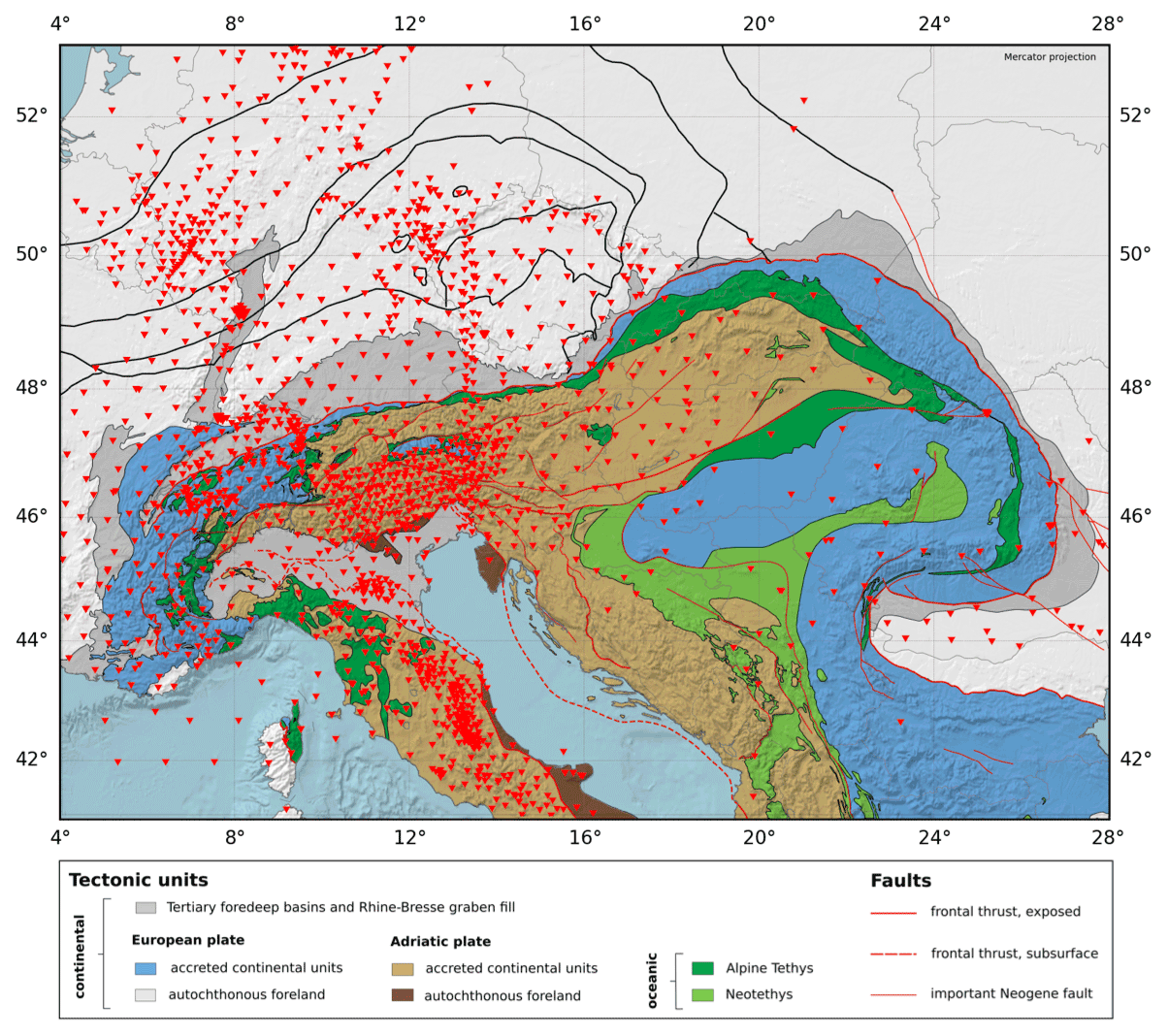
Figure 1 Distribution of permanent and temporary broadband stations used in this study (inverted red triangles) on a geological map of the area (following Hetényi et al., 2018a; their Fig. 1).

3 The profiles

In order to obtain high resolution along the profiles, we chose a size for the CCP area of 0.2^∘ in a direction parallel to the profiles. However, to keep the CCP area large enough for a sufficient number of traces to be used for the summation, we increased the extension of the CCP area perpendicular to the profile up to 1.0^∘ or more. Profiles with a smaller extension of CCP area perpendicular to the profile are shown in the Supplement for comparison. The locations of the chosen profiles are displayed in Fig. 2, and the corresponding seismic sections are shown in Figs. 3–14. The panels on the left side of the figures (labelled A) are for piercing points at 50 km, and the panels on the right side (labelled B) are for piercing points at 100 km depth. This means that the summation traces are best focused at these particular depths. The traces in the same geographical bins between A and B are not identical. Consequently, the left-hand panels focus on the Moho depth, while the right-hand panels point at discontinuities below the Moho. Each trace results from summing of at least 200 traces. The precursor time is given on the left scale relative to the SV arrival time. A depth scale is given on the right side of each figure. These depths were computed using the one-dimensional IASP91 global reference model. We provided the timescale in order to enable the use of alternative models for depth calculation. The amplitude scale is given relative to the amplitude of the incident SV signal. The latitude or longitude of the centre of each bin is given at the top of each figure. There is no overlapping between neighbouring traces along the profiles. The width of the profiles is given at the bottom of each figure.

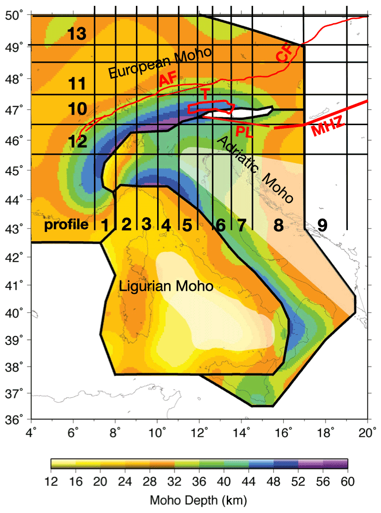
Figure 2 Moho map by Spada et al. (2013) with the locations of the sampling corridors used for profiles 1–13 shown in Figs. 3–14 and 20. The locations of the Mid-Hungarian Fault Zone (MHZ), the Periadriatic Line (PL), the Tauern Window (T), the Alpine Front (AF) and the Carpathians Front (CF) are also marked. The space between two black lines marks the width of the profile corridors.

The signals converted from S to P at the Moho are blue and denote an increase of velocity with increasing depth. Red signals denote a downward velocity decrease. As usual, the arrival times of the seismic signals must be picked in seismograms at the beginning of the signals and not at the signal maximum, as is usually the case for the classical receiver function method. Picking arrival times of weak emergent signals like converted waves from the Moho or deeper discontinuities is frequently a difficult problem, which we are still trying to improve. Therefore, so far we have only marked (using visual inspection) approximate Moho arrival times with dotted lines. A more accurate way to determine Moho arrival times would be a waveform correlation with the SV signal form, which we plan in the future. The signal forms of the Moho (and other) conversions are determined mainly by the signal forms of the incident SV signals. The response of the structure below the station (mainly the Moho interface) also contributes to the signal form. Below the Moho in the right-hand panels, we see concentrations of red signals for most of the profiles. These are caused by sharp or gradual downward velocity decreases. These signals below the Moho appear scattered and lack clear lateral correlations when compared to the Moho signals, which align much better. For this reason, we refer to the red regions below the Moho as zones of negative velocity gradients (NVGs). In some profiles we marked the bottom of a significant NVG group with a broad grey line that approximately indicates the arrival times of a group of scatterers. A negative seismic velocity gradient is often expected to mark the lithosphere–asthenosphere boundary. However, its depth depends on the nature of the geophysical measurements used to locate this boundary. Apart from temperature effects, this negative gradient may also be caused by changes in, for example, chemical composition or anisotropy (e.g. Eaton et al., 2009). Therefore, we prefer to use the neutral term NVG here.

4 Characteristic observations along the profiles

4.1 Moho structure

4.1.1 North–south profiles

We first present a series of north–south-oriented profiles shown in Figs. 3–9. In the entire region between 8.0 to 13.5^∘ E (profiles 2–6 in Figs. 4a–8a), we see a southward-dipping European Moho marked by dotted black lines. The Moho reaches its largest depth in profiles 2–6 at about 46.5^∘ N. This is near the latitude at which Spada et al. (2013) draw the boundary between the European and Adriatic Moho (see black line in Fig. 2) that roughly coincides with the location of the E–W-striking part of the Periadriatic Line west of longitude 13^∘ E. This implies that, according to geological evidence (Schmid et al., 2004; Kissling et al., 2006), the Moho south of about 46.5^∘ N, depicted in profiles 2–6, is the Adriatic Moho. In profiles 2–6, this Adriatic Moho rises towards a possible culmination located near 45.5^∘ N before descending southward beneath the Ligurian Moho at the front of the Apennines. This is shown by the onsets of the Adriatic Moho, which is also marked by dotted black lines (Figs. 4a–8a). At first sight, this geometry suggests a wedge-shaped trough below the Alpine chain. In fact, the two Mohos are separated from each other by a subduction corridor, whereby the European Moho indisputably dips southward beneath the Adriatic Moho according to geological and geophysical evidence (Schmid et al., 2004; Kissling et al., 2006), west of 11^∘ E. A far-reaching European Moho below the Adriatic Moho is, however, not observed in our data. This is different to the continental collision observed between India and Asia in Tibet, where a double Moho is observed and is interpreted as Indian lower crust reaching several hundred kilometres below the Tibetan crust (e.g. Yuan et al., 1997; Nabelek et al., 2009). East of 11^∘ E in the Alps, opinions about the subduction polarity have so far remained controversial (see discussion in Kästle et al., 2020). The maximum depth of the Moho reaches about 50 km near 8.5^∘ E (Fig. 4a) and increases to about 60 km near 13^∘ E (Fig. 8a). A very similar maximum Moho depth is also observed in the west near 7.5^∘ E. Here the Moho depth reaches about 65 km at about 45.5^∘ N (see profile 1 Fig. 3a). This Moho interface is hence located further south, which is caused by the south bending of the Alpine chain in the west (Fig. 2).

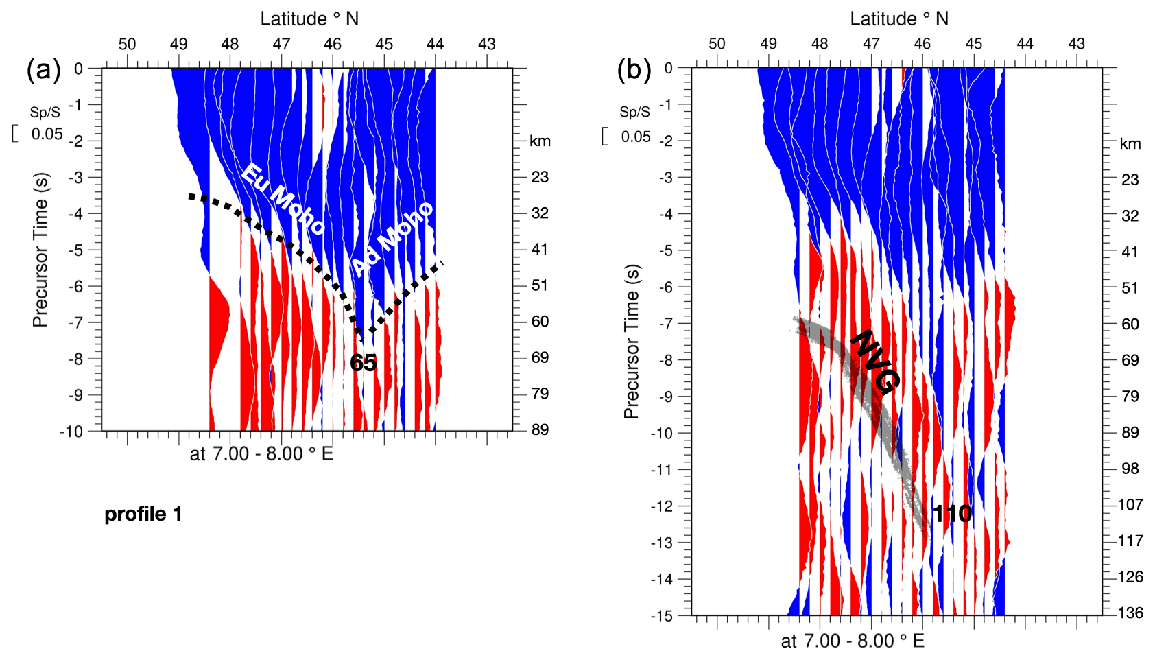
Figure 3 Profile 1. North–south profiles between 7–8^∘ E. Differential times of converted waves relative to the S arrival times are given on the left of sections (a) and (b). These times are converted into depth displayed on the right side of the sections using the global IASP91 velocity model. Blue colours indicate velocity increases with increasing depth (positive amplitudes), and red colours indicate velocity decreases (negative amplitudes). Note the vertical exaggeration of around 8.8 times. (a) Section of summation traces within bins of S-to-P piercing points at 50 km depth, appropriate for imaging the Moho. Bin size along the profile is 0.2^∘; the bin size perpendicular to the profile is given at the bottom of the section. The onsets of the S-to-P converted signals at the Moho are approximated by a dotted black line. “Eu Moho” refers to the European Moho, and “Ad Moho” designates the Adriatic Moho. The number given along the dotted black line in (a) indicates the greatest depth of the trough formed by the Moho signals. Panel (b) is the same as (a) but configured for a piercing point depth of 100 km, appropriate for imaging the mantle lithosphere below the Moho. A concentration of negative (red) signals marked NVG (negative velocity gradient) is visible below the Moho. The base of the NVG appears more scattered than the Moho. Therefore, the arrival times are only approximately marked by a scattered grey line. Similarly, the number given at the bottom of the NVG in (b) approximately marks the deepest extent of the NVG. Legends of the following figures with profiles refer to this figure.

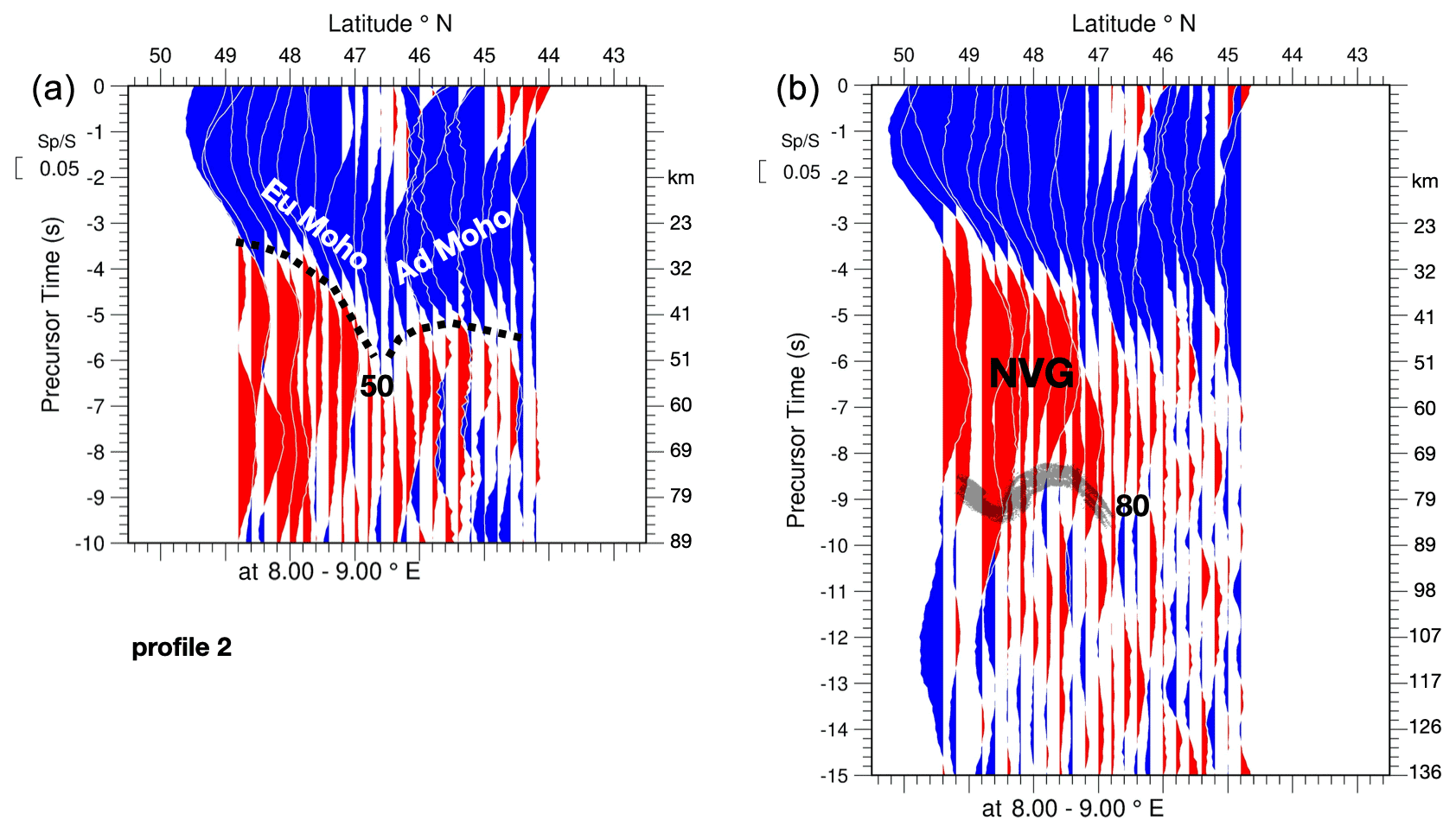
Figure 4 Profile 2. North–south profiles at 8–9^∘ E. Note that the deepest point of the Moho at 46.5^∘ latitude is slightly north the Europe–Adria boundary at around 46^∘ according to Spada et al. (2013) (see Fig. 2).

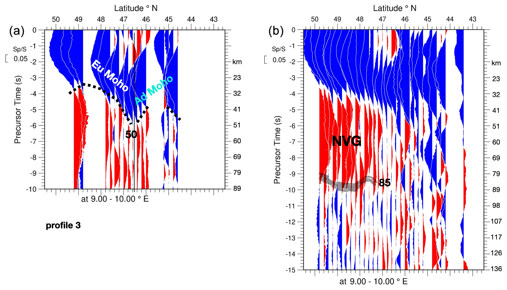
Figure 5 Profile 3. North–south profiles at 9–10^∘ E. Note that the deepest point of the Moho at 46.5^∘ latitude closely coincides with the Europe–Adria boundary according to Spada et al. (2013) (see Fig. 2).

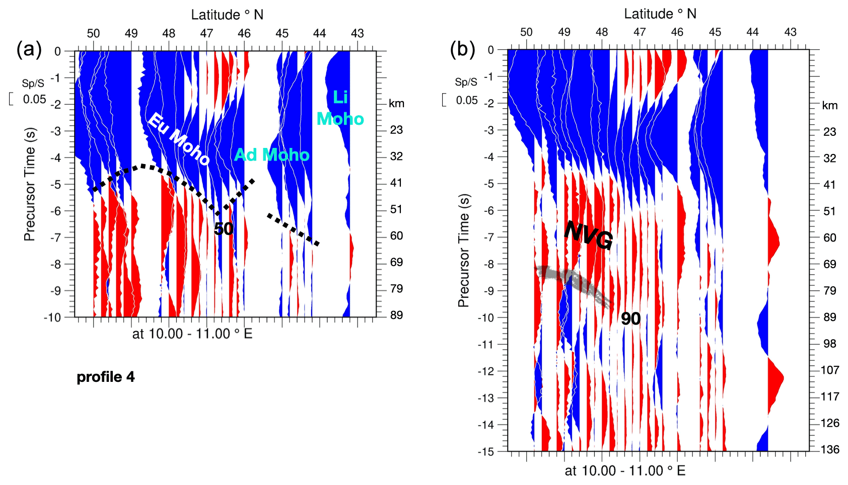
Figure 6 Profile 4. North–south profiles at 10–11^∘ E. Note that the deepest point of the Moho at 46.5^∘ latitude closely coincides with the Europe–Adria boundary according to Spada et al. (2013) (see Fig. 2). The base of the much shallower Ligurian Moho depicted in Fig. 2 marked “Li Moho” is visible at around 43.5^∘ latitude.

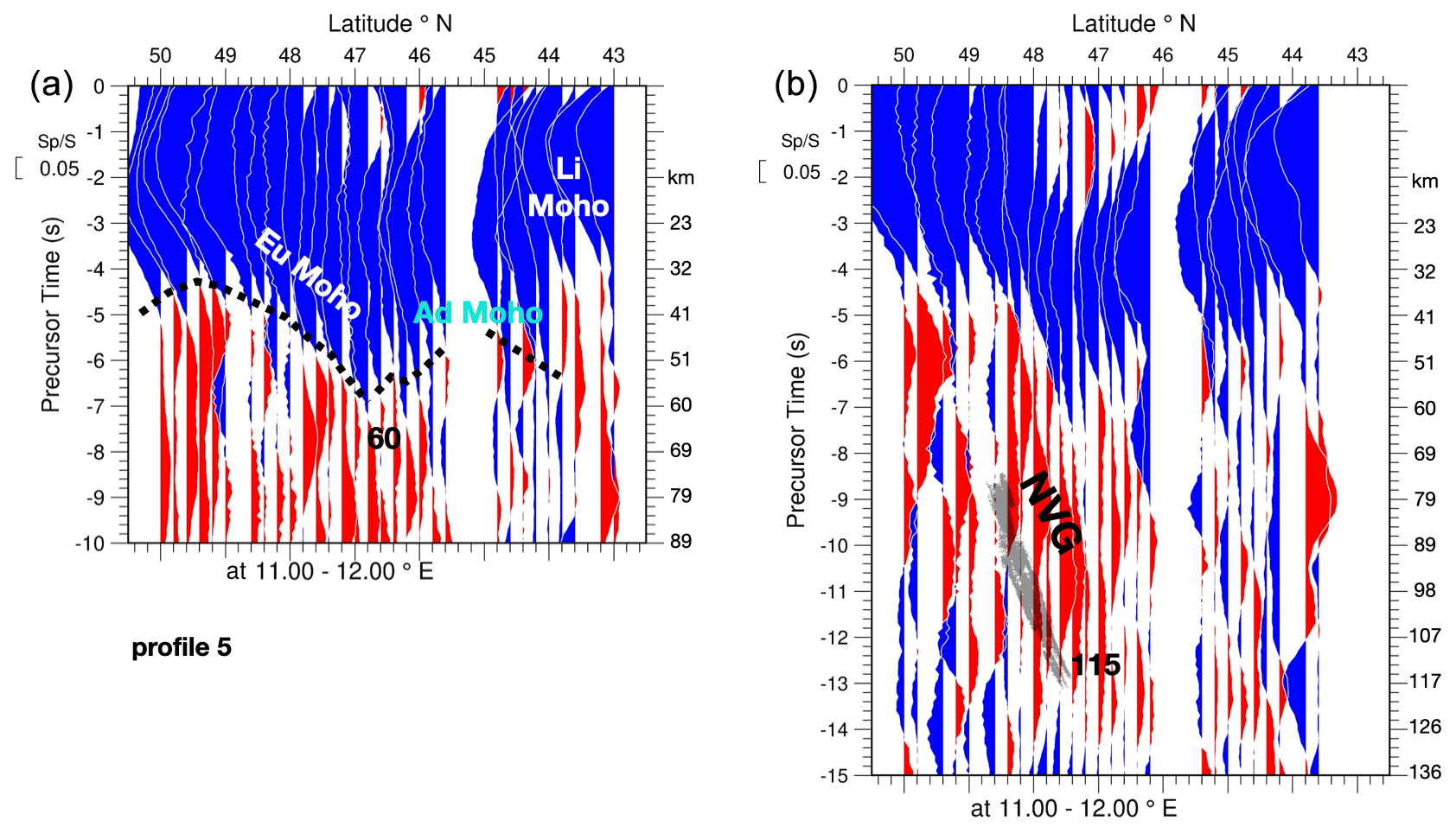
Figure 7 Profile 5. North–south profiles at 11–12^∘ E, i.e. near the western margin of the Tauern Window. Note that the deepest point of the Moho at 46.5^∘ latitude closely coincides with the Europe–Adria boundary according to Spada et al. (2013) (see Fig. 2). The base of the much shallower Ligurian Moho depicted in Fig. 2 marked “Li Moho” is visible at around 43.5^∘ latitude.

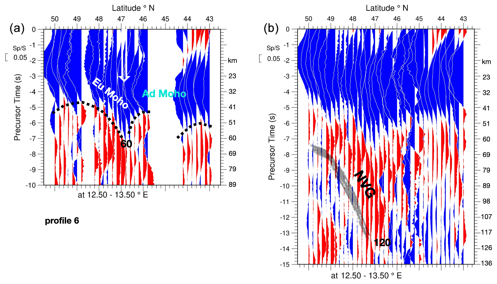
Figure 8 Profile 6. North–south profiles at 12.5–13.5^∘ E, i.e. across the eastern part of the Tauern Window. Note that the deepest point of the Moho near 47^∘ latitude, marked with a white arrow, closely coincides with the Europe–Adria boundary according to Spada et al. (2013) (see Fig. 2). This profile corridor does not reach the Ligurian Moho in the south.

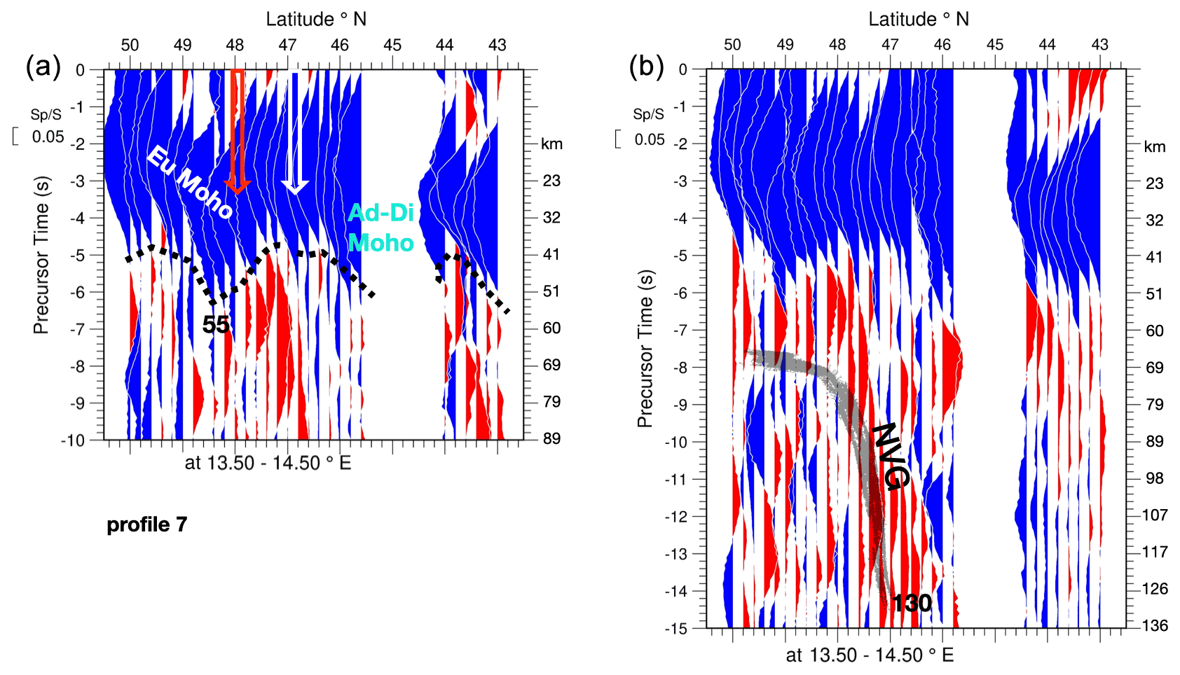
Figure 9 Profile 7. North–south profiles at 13.5–14.5^∘ E, located easterly adjacent to the Tauern Window. “Ad-Di Moho” indicates Adriatic–Dinarides Moho. (a) The white arrow located near 47^∘ indicates where the Moho reached the deepest point in profile 6 in Fig. 8. Note the abrupt along-strike change in terms of the Moho topography near 13^∘ E longitude, where this section shows the exact opposite, namely a culmination rather than a trough at this same latitude near 47^∘ (compare with Fig. 8). This location coincides with the white area in the map of Spada et al. (2013) denoting an area where the Moho is ill constrained by their data. The red arrow indicates the location of the frontal thrust of the Alpine orogen. (b) NVG denotes the location of one of the clearest NVG observations in the N–S profiles and the E–W profiles (see Fig. 12b).

A significant change in the structure of the Moho below the Alps is observed near 13^∘ E, i.e. near the eastern margin of the Tauern Window, by comparing Fig. 8a with Fig. 9a. West of this longitude the maximum depth of the Moho depression is around 60 km at 47^∘ N (white arrow in profile 6 of Fig. 8a). East of 13.5^∘ E the Moho depth at 47^∘ N is only about 40 km (white arrow in profile 7 in Fig. 9a), and the Moho depression near latitude 47^∘ seen in Fig. 8a is suddenly replaced by a culmination at the same latitude. This implies that the Moho topography no longer reflects a depression that would be expected to coincide with a scenario of subduction of the European plate below the Adriatic plate (or the opposite) in the Alps east of about 13^∘ E.

On the other hand, a thus far unknown substantial Moho depression similar to that observed at the plate interface west of 13^∘ E is observed further in the north (at 48–49^∘ N) in the profiles east of about 13^∘ E (see profiles 7–9 in Figs. 9a–11a). In the case of the profiles 7 and 8, this Moho depression is located north of the Alpine front (marked with red arrows in Figs. 9a and 10a; see also Fig. 2) and beneath the southern Bohemian Massif belonging to the European plate.

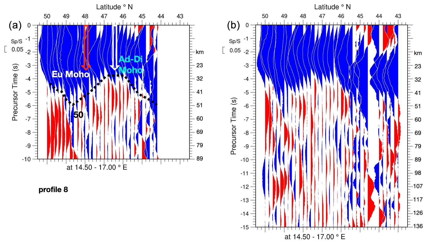
Figure 10 Profile 8. North–south profiles at 14.5–17^∘ E. As in profile 7 in Fig. 9, the Moho culminates near the junction of European and Adriatic Moho at latitude 46.5^∘ (i.e. at the Mid-Hungarian Fault Zone marked with a white arrow). Ad-Di denotes the Moho beneath the undeformed Adria plate dipping to the NE beneath the Dinarides. The red arrow indicates the location of the frontal thrust of the Alpine orogen.

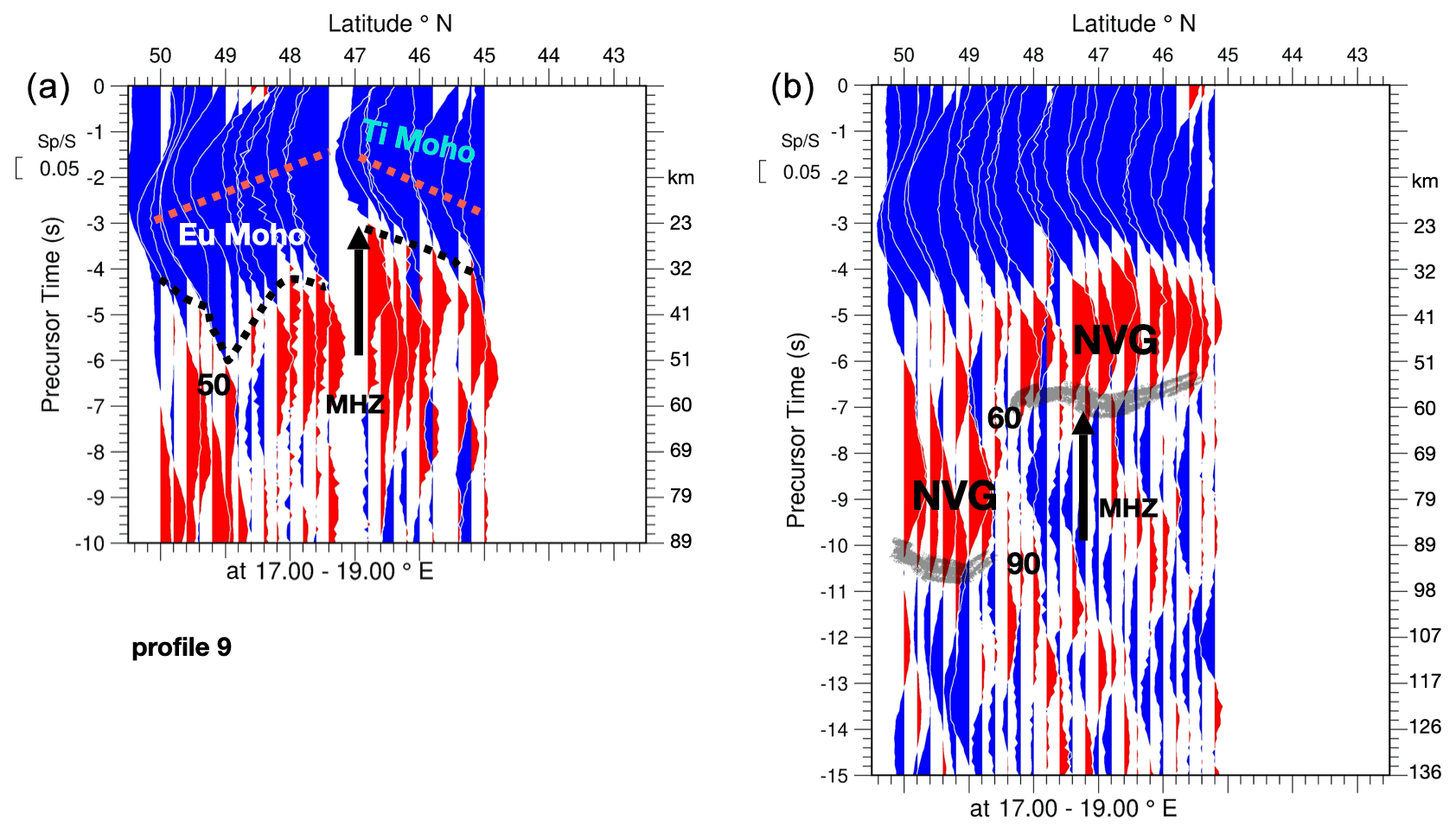
Figure 11 Profile 9. North–south profiles at 17–19^∘ E. As in the profile 8 in Fig. 10, the Moho culminates in the area of the Mid-Hungarian Fault Zone (MHZ) marked with a black arrow, located in the centre of the Pannonian Basin. In this profile the MHZ denotes the boundary of the substantially thinned European crust of the northern part of the Pannonian Basin with the shallow Moho of the southern part of the Pannonian Basin (south of lake Balaton, marked TI Moho) that belongs to the Tisza mega-unit (see Schmid et al., 2008). The dashed red line in (a) approximately marks the maxima of the Moho waveform.

In the very wide (between 17–19^∘ E) profile 9 (Fig. 11a) the Moho is observed to culminate in the area of the Pannonian Basin, combined with a jump in the Moho onset time that is seen near 47^∘ N and is marked with a black arrow. This occurs at the location of the Mid-Hungarian Fault Zone (MHZ in Fig. 2, e.g. Hetényi et al., 2015). North of this fault zone the Moho is at about 30 km and deepens to 50 km underneath the frontal Western Carpathians. South of the MHZ the Moho rises to about 25 km depth beneath the part of the Pannonian Basin located south of Lake Balaton. Moho depths of around 50 km have not been observed at the southern edge of the Bohemian Massif before. Hrubcová et al. (2005) and Wilde-Piórko et al. (2005) located the Moho in this region near 40 km depth based on seismic refraction data and receiver functions. Hetényi et al. (2015) observed a Moho depth of 25–30 km across the MHZ using P-receiver functions. Horváth et al. (2015) had obtained similar Moho depths from refraction lines. Szanyi et al. (2021) did not observe Moho signals in an ambient noise tomography study. The reason for such discrepancies regarding the Moho depths at the southern edge of the Bohemian Massif and around the MHZ could be as follows. If we look at the maxima of the Moho signals across the MHZ (marked approximately by the dotted red line in Fig. 11a), no significant jump is visible across the MHZ. We also note that the signal form of the Moho conversion is shorter south of the MHZ than north of it. Therefore, the earlier Moho onsets north of the MHZ might be explained by precursors of the actual Moho signal due to the existence of a second discontinuity located below the actual Moho north of the MHZ. The onset of the actual Moho could, in this case, not be adequately identified anymore. This phenomenon could also mean that the first arrivals identified as a Moho at the boundary of the Bohemian Massif could originate from a discontinuity below the Moho. Of course variations in the average crustal velocity change the Moho onset time. However, since the main part of the Moho signal remains unchanged across the MHZ, it seems likely that the average crustal velocity is also relatively unchanged.

We think that a better way to determine Moho onset times would be the comparison of the SV signal form with the Moho signal form, which we plan for a later time. In the Supplement (Figs. S9–S11) we present higher-resolution profiles across the MHZ, which, however, have a lower signal-to-noise ratio due to fewer traces in the stacking area. The influence of potentially different velocity models is not considered in the Moho depth estimates discussed above. Figure 15 summarises locations and maximum depths of the Moho along the Alpine chain in map view.

4.1.2 East–west profiles

In a second step we discuss the Moho depth shown along three east-west profiles presented in Figs. 12a–14a. Figure 12a shows profile 10, which is centred at 47^∘ N and entirely located on the European plate east of longitude 11.5^∘ E but straddles the plate boundary with Adria further to the east. This profile reaches the maximum Moho depth of around 60 km at about 13^∘ E, i.e. in the area of the Tauern Window (see Fig. 2). In the eastern direction, the Moho depth of this profile steadily rises to less than 20 km beneath the Pannonian Basin. West of its deepest point beneath the Tauern Window, the Moho also rises but exhibits a secondary depression between 7–8^∘ E located in the European plate near the Alpine Front (Fig. 2). For easier comparison, the dotted black line marking the Moho trend in Fig. 12a is copied into the neighbouring profiles 11 and 12, which are located north and south of profile 10, respectively (Figs. 13a and 14a). Profile 11 (Fig. 13a), located further north at 48^∘ N, runs entirely within the European plate and is similar to the one at 47^∘ N (Fig. 12a). However, in its western part the Moho is generally shallower in profile 11, probably due to the proximity to the Rhine Graben. Conversely, in the eastern part of profile 11 the Moho is generally deeper than that of profile 10 at 47^∘ N. This confirms the existence of a substantial Moho depression beneath the Bohemian Massif, which was found in the N–S profiles 7 and 8 (Figs. 9a and 10a). Profile 11 (Fig. 13a) also shows that the shallowing of the Moho towards the east is by far more moderate compared to that seen in profile 10. The southernmost E–W profile 12 at 46^∘ N (Fig. 14a) runs within the Adriatic plate east of 8.5^∘ E and shows a Moho trend that is very similar to the one at 47^∘ N (Fig. 12a). Only in its western part, running within the European part, is the Moho somewhat deeper.

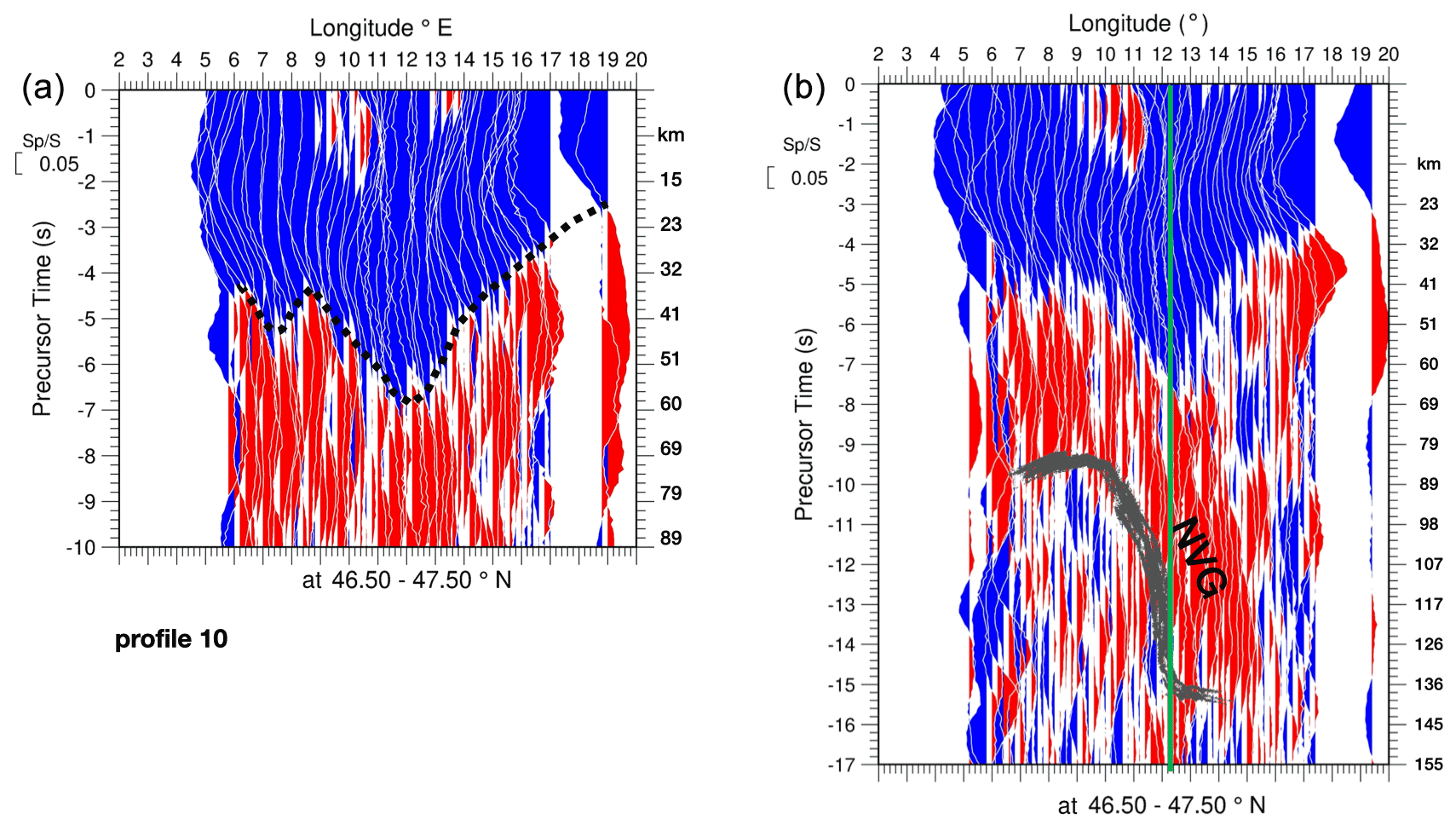
Figure 12 Profile 10. East–west profiles at 46.5–47.5^∘ N, largely running within the European plate and straddling the plate boundary east of 11.5^∘ E. Note the vertical exaggeration of around 13 times in this E–W profile and those of Figs. 13 and 14. (a) Approximate onsets of Moho signals along this profile are marked by a dotted black line. (b) The grey shadow indicates the base of the NVG; the vertical green line marks a very pronounced along-strike change at around 13^∘ E that is discussed in the text. Panel (b) shows the clearest observation in the entire area of the steeply dipping NVG.

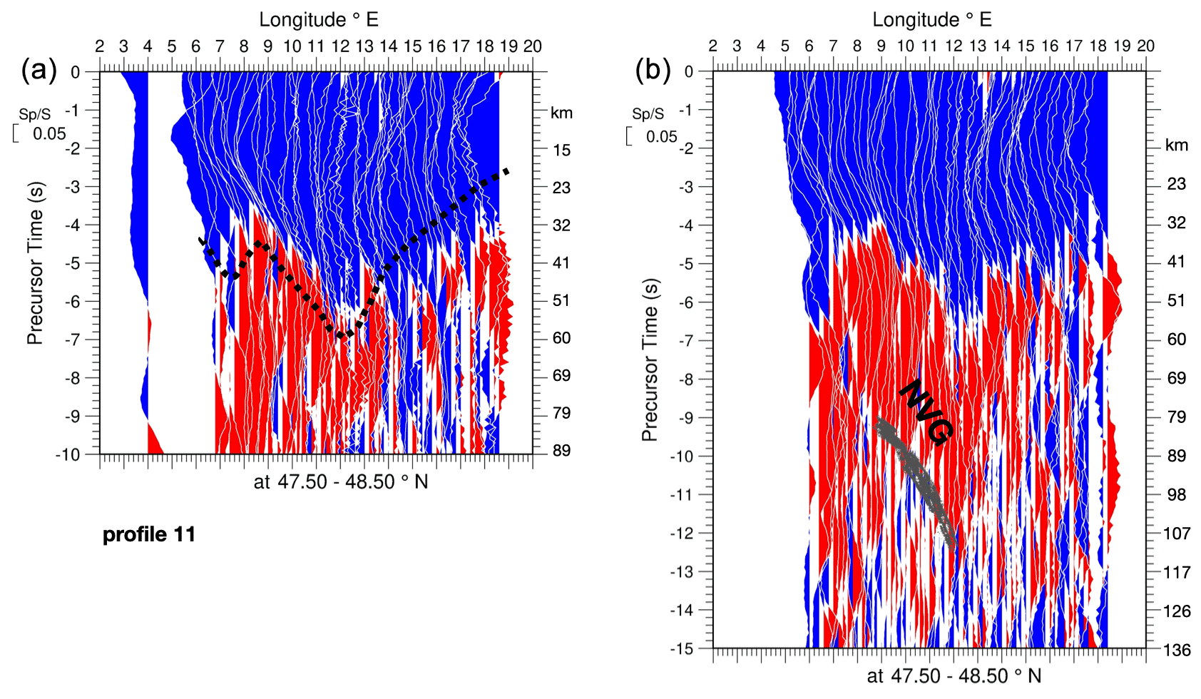
Figure 13 Profile 11. East–west profiles at 47.5–48.5^∘ N running entirely within the European plate. The same dotted black line as in profile 10 (Fig. 12) is copied into (a) for comparison.

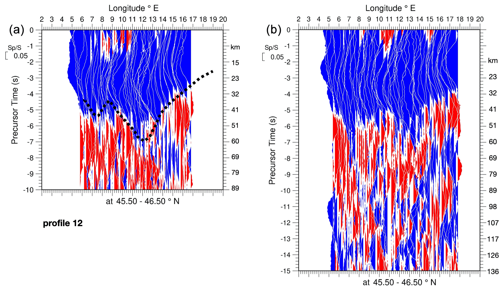
Figure 14 Profile 12. East–west profiles at 45.5–46.5^∘ N, running within the Adriatic plate east of 8^∘ E. The same dotted black line as in profile 10 (Fig. 12) is copied into (a) for comparison.

4.2 Structure within the uppermost mantle

The left and right panels of Figs. 3–14 show profiles of summed traces that have their piercing points within the same geographical bins. However, the piercing points are computed for different depths, namely 50 km for the left-hand panels and 100 km for the right-hand panels. Therefore, the summed traces in the bins are not identical. We now focus on the right panels computed by choosing a piercing point of 100 km, which is optimal when searching for structures in the shallow mantle below the Moho. Almost all Figs. 3b–14b show a relatively large number of negative signals (marked in red), indicating downward velocity reductions at some depth below the Moho. However, there are significant differences between these red signals compared to the blue signals marking the Moho. The amplitude of the Moho signals is nearly 10 % of the incident SV wave, whereas the amplitude of the negative signals from below the Moho is in most cases below 4 %. Moreover, in most cases the Moho signals mark a clear discontinuity, which can be correlated over the entire length of the profiles, whereas the negative signals from below the Moho do not mark a clear discontinuity but appear much more scattered. However, in parts of some of the profiles we were able mark the lower boundary of regions with exceptionally high concentrations of negative signals with a scattered grey line. We refer to such red regions as negative velocity gradient zones (NVG). The broad grey lines approximate the onset times of the scatterer group in this time window.

4.2.1 North–south profiles

An NVG could be mapped in profile 1 (Fig. 3b), dipping south down to about 110 km. In profiles 2–4 (Figs. 4b–6b, between 8–11^∘ E) the NVG is horizontal or slightly inclined to the south. The base of the NVGs is found at depths of 80–90 km, and they end towards the south at around latitude 47 to 48^∘, i.e. at or near the front of the Alps (see Fig. 2). This shows that they are definitely embedded in the European plate of the Alpine foreland, dipping southwards underneath the front of the Alps. In profiles 5–7 (Figs. 7b–9b, between 11–14.5^∘ E), the NVGs appear more pronounced. They are again southward dipping and their base reaches down to 115–130 km depth. They also end southward at around latitude 47^∘, which is somewhat further inside the Alps given the SSW–ENE strike of the Alpine front but still within the European plate (see Fig. 1). However, there is practically no significant indication of an NVG in profile 8 (Fig. 10b, 14.5–17^∘ E), i.e. in the area located well to the east of the Tauern Window spanning the Alps–Carpathians transition area (see Fig. 1). Note that profile 8, together with profile 9, was chosen to be relatively wide because of the scarcity of stations in the area. In the easternmost N–S profile (profile 9) east of 17^∘ E (Fig. 11b) running across the Western Carpathians and across the MHZ, a very different structure of the NVG is seen. The NVG is subhorizontal north of about 48.5^∘ N, where the base of the NVG shows a significant step moving up from 90 km beneath the European foreland and the external Carpathians to 60 km beneath the internal Carpathians and the Pannonian plain. We note that this jump in the depth of the NVG closely coincides with the onset of massive thinning of the lithosphere in the wider Pannonian realm that also affects the central Western Carpathians south of about 48.5^∘ (see Fig. 10 in Horváth et al., 2006).

4.2.2 East–west profiles

The east–west profile 10 centred along 47^∘ N (Fig. 12b) shows a very clear NVG that steeply dips eastward and reaches about 130 km depth at 13^∘ E where it turns horizontal and disappears near 14^∘ E. Comparing this easterly dip of the NVG in an E–W profile with its southerly dip in the N–S profiles at 11–14.5^∘ E (Figs. 7–9) shows that the NVG is in fact dipping towards the southeast. The east–west profile 11 along 48^∘ N (Fig. 13b) along the northern Alpine front also shows an apparently eastward-dipping NVG; however, it only reaches about 110 km depth at around 12^∘ E. Profile 12 along 46^∘ N (Fig. 14b) below the Po valley and located within the Adria plate in its eastern part lacks a similar eastward-dipping NVG. It seems astonishing that relatively steeply dipping structures can be imaged by steeply incident converted waves. Our interpretation is that the NVG area may contain a sufficient number of horizontal scatterers, which can be observed. The dip angle of the NVG might be biased (Schneider et al., 2013). Figure 16 summarises the deepest locations of the bottom of the NVG in the Spada (2013) Moho map and shows that they are all located in the area of the European plate. These deepest points are located (1) in the northern Alpine foreland (Bohemian Massif), (2) in the frontal part of the Western Carpathians, and (3) beneath the axial zone of the Central Alps and Eastern Alps, where they reach depths between 110 km and 130 in an area close to the southern margin of the European plate and in the vicinity of its contact with the Adria plate.

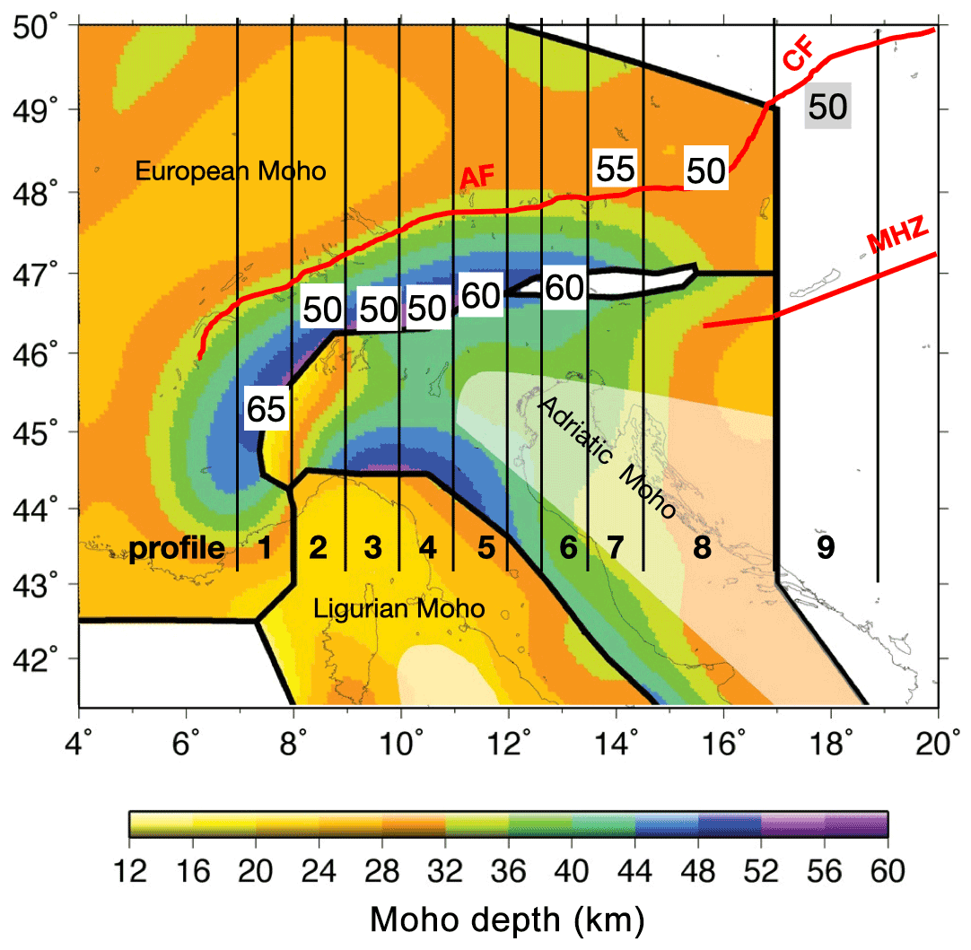
Figure 15 Moho map of Spada et al. (2013) indicating the provisional maximum recorded depths of the Moho along the Alpine chain west of 13.5^∘ E, below the southern part of the Bohemian Massif and below the northernmost Western Carpathians, marked in kilometres. These depths are still provisional because we still need to provide do a comparison of the Moho and SV waveforms for more accurate depth determinations in the future. Numbers are taken from profiles in Figs. 3a to 11a. AF, CF and MHZ mark the Alpine Front, Carpathian Front and Mid-Hungarian Fault Zone, respectively.

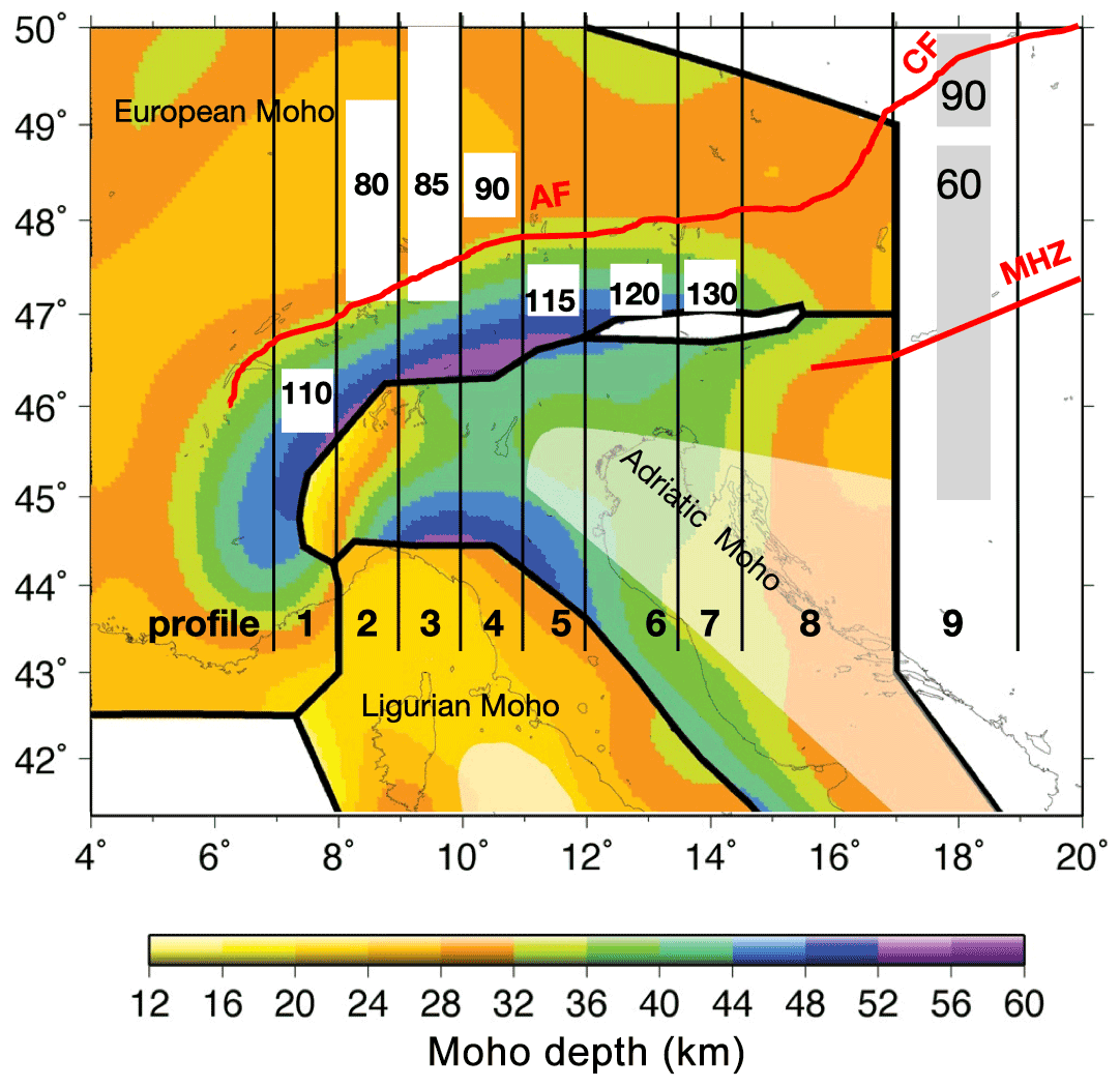
Figure 16 Moho map of Spada et al. (2013) indicating the provisional maximum recorded depth of the signals at the base of the NVG as marked in profiles 1–12 (b). Small white bins in the background of the numbers indicate steeply dipping NVG. Larger backgrounds indicate nearly horizontal NVG.

5 Comparison with earlier results

The comparisons of our results with those obtained by previous studies are discussed here and are displayed in Figs. 17–20.

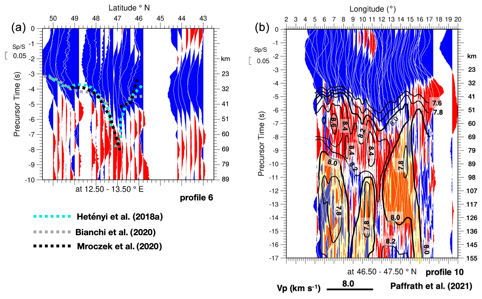
Figure 17 Copies of profiles 6 and 10, superposed with results of earlier studies for comparison. (a) Comparison of profile 6, focusing on Moho depth, with profiles of Hetényi et al. (2018b) based on P-receiver functions; Bianchi et al. (2021) based on PKP (core phases) crustal multiples; and Mroczek et al. (2020), also based on P-receiver functions. We did not mark Moho onsets in this figure as in Fig. 8a to allow comparison with the original data without our interpretation. (b) Comparison of profile 10, focusing on the depth of the base of the NVG indicated by a grey shadow in Fig. 12b, with absolute P-wave velocities obtained from teleseismic P-wave travel time tomography by Paffrath et al. (2021).

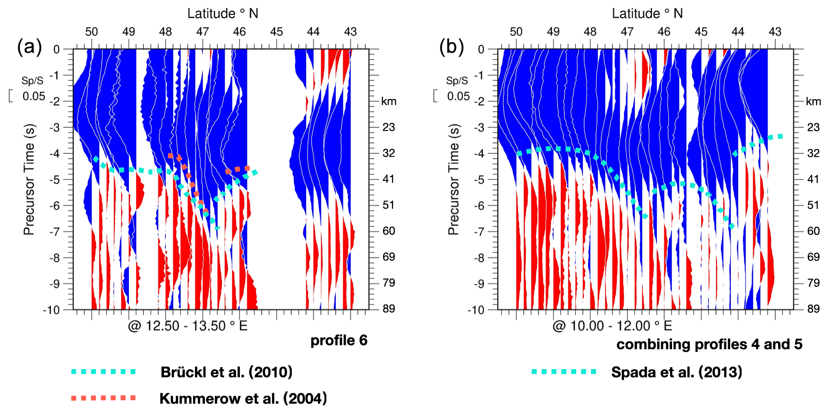
Figure 18 Copies of north–south profiles with results of earlier studies for comparison. (a) Comparison of profile 6 (Fig. 8a) with Brückl et al. (2010; their Fig. 3a), who used Moho data of Behm et al. (2007) based on wide-angle reflection and refraction data, and, with Kummerow et al. (2004) using the P-receiver function method. (b) Comparison of a combination of the corridors of profiles 4 and 5 (Figs. 6a and 7a) with the same profile taken from map of Spada et al. (2013).

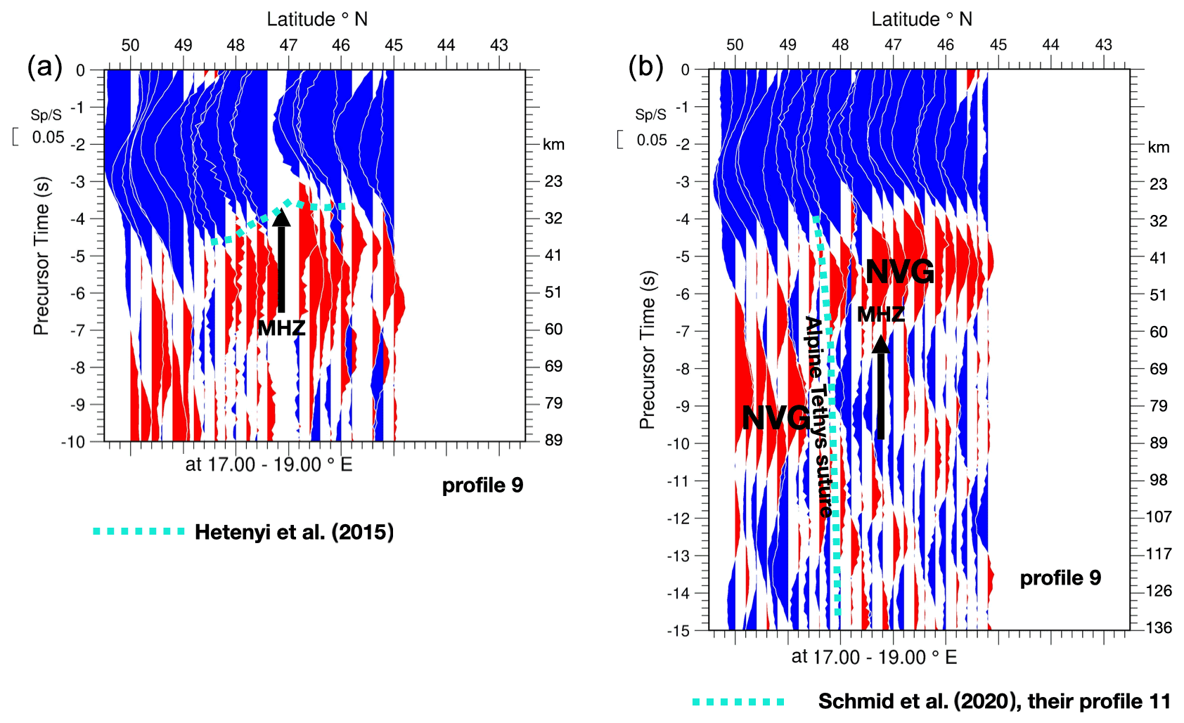
Figure 19 (a) Copy of profile 9 (Fig. 11a) across the MHZ superimposed with a study by Hetényi et al. (2015) who used P-receiver functions. (b) Copy of profile 9 (Fig. 11b) superimposed with the location of the Alpine Tethys suture as interpreted by Handy et al. (2021) based on mantle tomography by Paffrath et al. (2021).

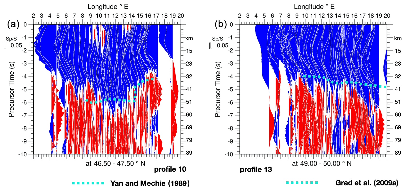
Figure 20 (a) Copy of profile 10 (Fig. 12a) with results of Yan and Mechie (1989), who used data from a refraction profile along the Alpine chain. (b) Additional east–west profile well north of the earlier profiles shown, constructed for comparison with the Moho map of Grad et al. (2009a) and comparison with profile 10 of Fig. 20a. Note the substantial difference in Moho depth between our data east of 14^∘ E and those of Grad et al. (2009a). Also note that we see pronounced Moho deepening towards the east in this northerly located profile located in the European lithosphere, which contrasts with Moho shallowing towards the east in the southern profile of Fig. 20a located in the Pannonian region (see Fig. 2 for the location of the profiles).

In Fig. 17a we compare our Moho data obtained along the north–south profile 6 centred at 13^∘ E (Fig. 8) with the results of Hetényi et al. (2018b) and Bianchi et al. (2021) along their profile at 13.3^∘ E (temporary passive experiment EASI). Hetényi et al. (2018b) used P-receiver function data from this profile between the Eger Rift in the northern part of the Bohemian Massif and the Adriatic Sea. Their recorded Moho depth is plotted as dotted cyan line along our Sect. 6 in Fig. 17a. Their Moho depth increases from 25 km at the Eger Rift at the northern end to about 30 km at the Alpine front at 48^∘ N. From there the European Moho deepens rapidly to about 60 km at 47^∘ N below the Tauern Window. The northward-dipping Adriatic Moho reaches deeper down to 70 km and dips below the European Moho according to these authors. This is not seen in our results. The very general shape of the Moho is nevertheless in good agreement with our data. However, their depths of the European and Adriatic Moho are about 5 km shallower than ours, except near the deepest point at 47^∘ N. This might partly be due to the different velocity models used. Hetényi et al. (2018b) used a local model, whereas we used a global model (IASP91). Our data do not support the postulate of Hetényi et al. (2018b) that the Adriatic Moho in the Eastern Alps dips northward underneath the European Moho. Instead, our Moho depression looks rather symmetric, similar to Spada et al. (2013). Bianchi et al. (2021) used PKP multiples within the crust below the seismic stations to derive the Moho depth. Their results are marked by a slight dotted grey line in Fig. 17a. The agreement between our data with those of Bianchi et al. (2021) is also reasonably good, except near 47^∘ N, where they have no data. It should also be noted that the “Moho gap” mapped in white by Spada et al. (2013) at 47^∘ N (Fig. 2) does not seem to exist according to our data, similar to the findings of Mroczek et al. (2020) and Hetényi et al. (2018b).

In Fig. 17b, depicting the E–W profile 10, we compare our data regarding the NVG in the upper mantle below the Moho (previously discussed and illustrated in Fig. 12b) with results from the teleseismic body wave tomography by Paffrath et al. (2021) by superimposing the P-wave velocity contours that these authors used for calculating velocity anomalies along the same E–W profile 10. There is fairly good agreement between the two data sets in the western part of the profile between 5 and 12^∘ E. In this area the eastward-dipping base of the red NVG zone roughly coincides with the top of an area associated with abnormally low P-wave velocities below 8.0 km s⁻¹ marked in yellow in the western part of the profile. This same NVG zone was also traversed by the N–S profiles of profiles 4 to 7 (Figs. 6–9) that show the NVG zone to be hosted within the SE-dipping European plate. However, while the data of Paffrath indicate a major change to occur already east of longitude 12^∘ E, where the mantle tomography indicates eastward shallowing of the top of the zone of low P-wave anomalies, our NVG zone hosted in the European lithosphere can be followed until longitude 12^∘ E (green line in Fig. 12b), terminating at around 15^∘ E. Hence, the agreement between the two methods is poor between 12 and 14^∘ E. Further studies and high-resolution S-wave velocity models are needed to resolve this discrepancy. In this context it should, however, be noted that our method of using converted waves is sensitive to velocity gradients and not absolute velocities. This means that smaller-scale relative velocity reductions could well be embedded in larger high- or low-velocity regions. Further studies and high-resolution S-wave velocity models are needed to resolve this discrepancy. In spite of the discrepancies between the two data sets in the 12–14^∘ E sector, the data of Paffrath et al. (2021) confirm that a first-order lateral change occurs in the area of the Tauern window. East of this area the SE dip of the European lithosphere laterally terminates, giving way to a different scenario that indicates eastward shallowing of the Moho (our data) that coincides with the lateral disappearance of the NVG (see yellow area marking velocities $<\mathrm{8.0}\mathrm{km}{\mathrm{s}}^{-\mathrm{1}}$ in Fig. 17b) according to the velocities provided by the model of Paffrath et al. (2021).

Geissler et al. (2010) presented a map of (what was called) the lithosphere–asthenosphere boundary (LAB) of central Europe obtained from an S-receiver function study (their Fig. 9). We compare their LAB observations with our NVG observations in the Eastern Alps. They used the classical S-receiver function method with deconvolution before stacking, whereas we use stacking of the original untouched broadband data. Our east–west profile 10 (Fig. 12) between 46.5 and 47.5^∘ N approximately covers their profiles I and J (Fig. 9, Geissler et al., 2010). We see in profile 10 between about 12 and 15^∘ E a steeply eastward-dipping NVG reaching from about 90 to 140 km depth. They observe in approximately the same area an eastward-dipping LAB from about 100 to 150 km depth. This can be considered a very good agreement taking into account the different stacking areas used in both studies. Geissler et al. (2010) used a $\mathrm{1}{}^{\circ }\times \mathrm{1}{}^{\circ }$ area. We used a stacking area of 1^∘ latitude and 0.2^∘ longitude, since we had more data available, which resulted in higher resolution. We note that the area where we observe this steeply eastward-dipping NVG, which confirms similar observations by Geissler et al. (2010), is practically the same area where Lippitsch et al. (2003) observe a north-east dipping slab in a tomography study.

Figure 18a compares our north–south Moho profile 6 with the Eastern Alps Moho profile by Behm et al. (2007) and Brückl et al. (2010) at 13^∘ E. The agreement of the profiles is very good. The general conclusion of Brückl et al. (2010) that the European Moho is subducting below the Adriatic Moho is not obvious from our data, but the asymmetry in our data is in favour of this conclusion. Our data compare fairly well with the data of Kummerow et al. (2004) along their profile at 12^∘ E (which is about 80 km further west), although their Moho depths appear shallower. In Fig. 18b we compare our north–south profile along a corridor between 10 and 12^∘ E with a profile in the map of Spada et al. (2013) (see Fig. 2) at 11^∘ E. The agreement between the two data sets is good. North of 47^∘ N our Moho seems to be in average about 5 km deeper. The reason is not exactly known. This might be caused by differences in the background models used for the time–depth migration. The Moho jump near 44^∘ N marking the transition from the Adriatic to the Ligurian Moho is evident on both profiles.

In Fig. 19a we compare our Moho data along profile 9 (Fig. 11a) depicting a culmination of the Moho with the receiver function data of Hetényi et al. (2015) by projecting the northwest–southeast profile of Hetényi et al. (2015) onto our north–south profile. This same Moho culmination follows the strike of the MHZ and was traced further to the ENE by Kalmár et al. (2019). North of the MHZ the Moho is rapidly deepening towards the north. Figure 19b compares our profile 9 (Fig. 11b) with mantle tomographic results from Paffrath et al. (2021), geologically interpreted by Handy et al. (2021). The NVG in Fig. 19b to both sides of the MHZ, which is very shallow and located immediately below the Moho, is not changing depth across the MHZ at 47^∘ N where the Moho starts to deepen (see Fig. 19a). Rather, an offset of the NVG to greater depth occurs at around 48.5^∘ N, which is located within the central Western Carpathians, i.e. north of the Pannonian Basin. The comparison with the tomographic data shows that this jump in depth of the NVG coincides with the location of the Alpine–Tethys suture zone identified in tomography data (Handy et al., 2021), a zone that forms the southern boundary of the European lithosphere (dotted subvertical green line in Fig. 19b). Our data reinforce the fundamental difference between the seismic properties of the European lithosphere beneath the frontal Western Carpathians with those of the more internal parts of the Western Carpathians and the Pannonian realm characterised by a shallow lithosphere–asthenosphere boundary (e.g. Horváth et al., 2006; Kind et al., 2017).

In Fig. 20a we compare our Moho depth profile along the east–west profile 10 at 47^∘ N (Fig. 12a) with early results of seismic refraction experiments (Yan and Mechie, 1989). The agreement in the general trend of eastward shallowing starting in western Tauern Window at around 12^∘ E is good. Figure 20b presents an additional profile 13 located north of profile 11 at 49–50^∘ N in the European lithosphere crossing the front of the Western Carpathians at 17.5^∘ E (Fig. 2), added for comparison with the Moho map of Grad et al. (2009a), based on a variety of geophysical data. The dotted cyan line in Fig. 20b marks the rapid eastward Moho deepening towards the front of the Western Carpathians initiating at ca. 14^∘ E and reaching 50 km below the external Western Carpathians. The discrepancy with the data of Grad et al. (2009a) is considerable in the easternmost part of this profile, where our data show a much more pronounced deepening of the Moho. This eastward deepening along the northerly profile of Fig. 20b strongly contrasts with the eastward shallowing of the Moho shown in Fig. 20a, i.e. in a more southerly profile (at 46.5–47.5^∘ N) crossing the area of the northern margin of the Pannonian plain around the MHZ. This marked difference is due to the fact that in our data the Moho in the profile of Fig. 20b is located in the European lithosphere, which bends down across the SW–NE-striking front of the Western Carpathians (see Fig. 2), while the profile of Fig. 20a runs within the Pannonian realm characterised by the eastward-shallowing Moho depth shown in E–W profiles 10, 11 and 12, caused by Miocene backarc extension in the Pannonian Basin, along the MHZ and in the internal parts of the Western Carpathians region (Horváth et al., 2015).

6 Summary of observational results

The comparison with results from other studies using other methods shows that by using broadband S-to-P converted signals we are able to obtain clear images of the Moho topography along most of the Alpine chain and also reveal the presence of some features that were not detected before. Furthermore, this method allows highlighting an important along-strike change regarding Moho topography that takes place at around 13^∘ E, i.e. in the eastern Tauern Window. The Moho depression beneath the Central Alps along the Europe–Adria lithosphere boundary along 47^∘ N deepens from some 50 km at 8^∘ E to 60 km at around 13^∘ E. In the N–S profiles the Moho depression very abruptly gives way to an up-doming of the Moho along the axial zone of the Alpine orogen at around 13^∘ E, persisting all the way into the Pannonian Basin, as the depth of the Moho generally decreases to <30 km N and S of 47^∘ N as well. Our data also indicate the existence of a substantial Moho depression east of 13^∘ E and near the Alpine frontal thrust extending eastward into the area of the frontal Western Carpathians whose extent has so far remained undetected (see Fig. 15).

In the shallow mantle we also observe, extending from 10 to 14^∘ E along an E–W section along 47^∘ N combined with N–S sections, steeply SE-dipping areas of downward velocity reductions referred to as NVGs that extend to at least 140 km depth at 14^∘ E and disappear east of there. The base of the NVG, which roughly coincides with the top of a low-velocity zone revealed by mantle tomography west of 12^∘ E (Paffrath et al., 2021), is related to the European slab. The termination of the NVG at 14^∘ E suggests an important along-strike change also in terms of the shallow mantle structure taking place at 14^∘ E, i.e. about 1^∘ east of the along-strike change observed for the Moho topography. Below the frontal Western Carpathians at about 49^∘ N we observed a jump of the base of the subhorizontal NVG from about 60 km in the south to 90 km in the north.

7 Discussion and conclusions

From a technical point of view the improved images of the present paper are, besides the obvious reason of using much larger amounts of data, also due to the modified data processing technique. In the receiver function technique seismic traces are sometimes filtered without paying sufficient attention to sidelobes or acausality. Another problem is the waveform compression caused by deconvolution and summation along the maximum of the compressed signals, which also produces sidelobes that tend to be misinterpreted. We therefore avoided all filtering and lined up the traces along the onsets of the S signals for summation. We found good agreement between our results and earlier results obtained in many regions. This emphasises the reliability of our results. We also think that using additional seismic phases could help to increase the reliability of the seismic images and as a consequence also that of the tectonic interpretation. A good example is the usage of PKP multiples below the stations as shown by Bianchi et al. (2021).

From the geological point of view the Moho topography reflects deeper subduction of the European lithosphere only west of and in the Tauern Window area. This is no more the case east of 13^∘ E, i.e. east of the eastern Tauern Window, where the Moho is up domed in the contact area between the European and the Adriatic lithosphere. According to geological evidence (Ratschbacher et al., 1991) and according to the geological interpretation of recent mantle tomographic data (Paffrath et al., 2021; Handy et al., 2021) this updoming is likely due to a late-stage modification of the Moho topography in the Eastern Alps, the Western Carpathians and the Pannonian Basin that occurred during the last ca. 20 Myr. Such updoming goes together with crustal thinning associated with lateral extrusion of the so-called ALCAPA (Alpine, Carpathian, Pannonian) mega-unit associated with the N-directed indentation of the Dolomites indenter and roll back of the Eastern Carpathians (Ratschbacher et al., 1991). The rapid jump of the base of the NVG from about 60 km in the south to 90 km in the north below the frontal West Carpathians at about 49^∘ N is also related to extension and asthenosphere upwelling in the Pannonian Basin that also affected the internal Western Carpathians (Horváth et al., 2015).

The following three main additional new salient features are of importance: (1) the possible existence of a second discontinuity below the Moho north of the Mid-Hungarian Fault Zone emphasises the important role this fault zone played in terms of lateral offsets that occurred during the lateral extrusion of ALCAPA during the Miocene (Schmid et al., 2008). (2) A second Moho trough was detected north of the Alps, reaching down to about 50 km depth and located in the Bohemian Massif north of the Alpine front in the Eastern Alps, extending eastward into the frontal part of the Western Carpathians. This structure, hosted in the European lithosphere, has not been observed before and cannot be interpreted yet at this stage. Further studies are needed to clarify this structure. (3) We observed areas of downward velocity reductions referred to as NVGs hosted within the European lithosphere in the foreland of the Alps at a depth of 80–90 km. In the Eastern Alps west of 14^∘ E these NVGs can be traced down to depths of 115–140 km all the way to 47^∘ N, i.e. into the axial zone of the Alps (marked NVG in Figs. 9b and 12b).