Thermal non-equilibrium of porous flow in a resting matrix applicable to melt migration: a parametric study

Fluid flow through rock occurs in many geological settings on different scales, at different temperature conditions and with different flow velocities. Depending on these conditions the fluid will be in local thermal equilibrium with the host rock or not. To explore the physical parameters controlling thermal non-equilibrium, the coupled heat equations for fluid and solid phases are formulated for a fluid migrating through a resting porous solid by porous flow. By non-dimensionalizing the equations, two non-dimensional numbers can be identified controlling thermal non-equilibrium: the Péclet number Pe describing the fluid velocity and the porosity ϕ. The equations are solved numerically for the fluid and solid temperature evolution for a simple 1D model setup with constant flow velocity. This setup defines a third non-dimensional number, the initial thermal gradient G, which is the reciprocal of the non-dimensional model height H. Three stages are observed: a transient stage followed by a stage with maximum non-equilibrium fluid-to-solid temperature difference, ΔT_max, and a stage approaching the steady state. A simplified time-independent ordinary differential equation for depth-dependent (T_f−T_s) is derived and solved analytically. From these solutions simple scaling laws of the form $\left(T_{\mathrm{f}}-T_{\mathrm{s}}\right)=f\left(\mathit{Pe},G,z\right)$ are derived. Due to scaling they do not depend explicitly on ϕ anymore. The solutions for ΔT_max and the scaling laws are in good agreement with the numerical solutions. The parameter space PeG is systematically explored. Three regimes can be identified: (1) at high Pe ($>\mathrm{1}/G$) strong thermal non-equilibrium develops independently of Pe, (2) at low Pe ($<\mathrm{1}/G$) non-equilibrium decreases proportional to decreasing Pe⋅G, and (3) at low Pe (<1) and G of the order of 1 the scaling law is $\mathrm{\Delta }{T}_{max}\approx \mathit{Pe}$. The scaling laws are also given in dimensional form. The dimensional ΔT_max depends on the initial temperature gradient, the flow velocity, the melt fraction, the interfacial boundary layer thickness, and the interfacial area density. The time scales for reaching thermal non-equilibrium scale with the advective timescale in the high-Pe regime and with the interfacial diffusion time in the other two low-Pe regimes. Applying the results to natural magmatic systems such as mid-ocean ridges can be done by estimating appropriate orders of Pe and G. Plotting such typical ranges in the Pe–G regime diagram reveals that (a) interstitial melt flow is in thermal equilibrium, (b) melt channeling such as revealed by dunite channels may reach moderate thermal non-equilibrium with fluid-to-solid temperature differences of up to several tens of kelvin, and (c) the dike regime is at full thermal non-equilibrium.

1 Introduction

Fluid flow through rock occurs in many geological settings on different scales, at different temperature conditions and with different flow velocities. Depending on these conditions the fluid will be in local thermal equilibrium with the host rock or not. On a small scale, e.g., grain scale, usually thermal equilibrium is valid. Examples include melt migration through a porous matrix in the asthenosphere or in crustal magmatic systems at super-solidus temperatures (e.g., McKenzie, 1984), groundwater or geothermal flows in sediments or cracked rocks (e.g., Verruijt, 1982; Furbish, 1997; Woods, 2015), or hydrothermal convection in the oceanic crust (e.g., Davis et al., 1999; Harris and Chapman, 2004; Becker and Davies, 2004). On a somewhat larger scale local thermal equilibrium may not always be reached. Examples of such flows include melt migration in the mantle or crust at temperatures close to or slightly below the solidus where melt may be focused and migrates through systems of veins or channels (Kelemen et al., 1995; Spiegelman et al., 2001). Within the upper oceanic crust water may also migrate through systems of vents or channels (Wilcock and Fisher, 2004). At even larger scales and at sub-solidus conditions, magma rapidly flows through propagating dikes or volcanic conduits (e.g., Lister and Kerr, 1991; Rubin, 1995; Rivalta et al., 2015) and is locally at non-equilibrium with the host rock.

Heat transport associated with most of such flow scenarios is usually described by assuming thermal equilibrium between the fluid and solid under slow flow conditions (e.g., McKenzie, 1984). Alternatively, for more rapid flows such as melts moving in dikes through a cold elastic or visco-elasto-plastic ambient rock, the fluids are assumed to be isothermal (e.g., Maccaferri et al., 2011; Keller et al., 2013). However, on a local scale of channel or dike width, thermal interaction between rising hot magma and cold host rock is important and may lead to effects such as melting of the host rock and freezing of the magma with important consequences for dike propagation and the maximum ascent height (e.g., Bruce and Huppert, 1990; Lister and Kerr, 1991; Rubin, 1995). Clearly, in such rapid fluid flow scenarios melt is not in thermal equilibrium with the ambient rock.

Thus, there exists a transitional regime, which, for example, may be associated with melt focusing into pathways where flow is faster and thermal equilibrium might not be valid anymore. In such a scenario it might be possible that channelized flow of melt might penetrate deeply into sub-solidus ambient rock, and thermal non-equilibrium delays freezing of the ascending melts and promotes initiation of further dike-like pathways. Indeed, for mid-oceanic ridges compositional non-equilibrium has proven to be of great importance for understanding melt migration and transport evolution (Aharonov et al., 1995; Spiegelman et al., 2001). Thus, it appears plausible that in cases of sufficiently rapid fluid flow, e.g., due to channeling or fracturing, thermal non-equilibrium may also become important. Describing this non-equilibrium macroscopically, i.e., on a scale larger than the pores or channels, is the scope of this paper.

While the physics of thermal non-equilibrium in porous flow is well studied in more technical literature (e.g., Schumann, 1929; Spiga and Spiga, 1981; Kuznetsov, 1994; Amiri and Vafai, 1994; Minkowycz et al., 1999; Nield and Bejan, 2006; de Lemos, 2016), so far it has attracted only little attention in the geoscience literature, but see Schmeling et al. (2018) and Roy (2020). The basic approach in all these studies is the decomposition of the heat equation for porous flow into two equations, one for the solid and one for the migrating fluid. The key parameter for thermal non-equilibrium is a heat exchange term between fluid and solid, which appears as a sink in the equation for the fluid and as a source in the equation for the solid. Usually, this heat exchange term is assumed proportional to the local temperature difference between fluid and solid (Minkowycz et al., 1999; Amiri and Vafai, 1994; de Lemos, 2016; Roy, 2020). However, Schmeling et al. (2018) showed that in a more general formulation the heat exchange term depends on the complete thermal history of the moving fluid through the possibly also moving solid. Here we will follow the common assumption and use the local temperature difference formulation. While Schmeling et al. (2018) showed that the magnitude of thermal non-equilibrium essentially depends on the flow velocity, or more precisely on the Péclet number, here we will more generally explore the parameter space.

While thermal non-equilibrium of an arbitrary porous flow system depends on many parameters, our approach is to reduce the complexity of the system and systematically explore the non-dimensional parameter space. It will be shown that only two non-dimensional parameters control thermal non-equilibrium in porous flow, namely the Péclet number and the porosity. In our simple 1D model setup with constant flow velocity a third non-dimensional number, the non-dimensional initial thermal gradient G, is identified, which is equal to the reciprocal non-dimensional model height $H=\mathrm{1}/G$. The non-dimensionalization allows application of the results to arbitrary magmatic or other systems. The aim is to derive scaling laws that allow an easy determination of whether thermal equilibrium or non-equilibrium is to be expected and quantitatively to estimate the maximum temperature difference between fluid and matrix. The results will be applied, the magmatic system of a mid-ocean ridge setting.

2 Governing equations and model setup

2.1 Heat conservation equations

We start with considering a general two-phase matrix–fluid system with variable properties and solid and fluid velocities and subsequently apply simplifications. The two phases are incompressible, and we assume local thermal non-equilibrium conditions; i.e., the two phases exchange heat. The equations for conservation of energy of this system are given by de Lemos (2016), for example. Assuming constant pressure, the conservation of energy of the fluid phase is given by

$$\begin{array}{}\text{(1)}& c_{p,\mathrm{f}}\left({\displaystyle \frac{\partial \left(\mathit{\varphi }{\mathit{\rho }}_{\mathrm{f}}{T}_{\mathrm{f}}\right)}{\partial t}}+\mathrm{\nabla }\cdot \left(\mathit{\varphi }{\mathit{\rho }}_{\mathrm{f}}{v}_{\mathrm{f}}{T}_{\mathrm{f}}\right)\right)=\mathrm{\nabla }\cdot \left(\mathit{\varphi }{\mathit{\lambda }}_{\mathrm{f}}\mathrm{\nabla }{T}_{\mathrm{f}}\right)-Q_{\mathrm{fs}}.\end{array}$$

For the definition of all quantities, see Table 1. Equation (1) can be rearranged into

$$\begin{array}{}\text{(2)}& \begin{array}{rl}& c_{p,\mathrm{f}}\left(T_{\mathrm{f}}{\displaystyle \frac{\partial \left(\mathit{\varphi }{\mathit{\rho }}_{\mathrm{f}}\right)}{\partial t}}+\mathit{\varphi }{\mathit{\rho }}_{\mathrm{f}}{\displaystyle \frac{\partial T_{\mathrm{f}}}{\partial t}}+T_{\mathrm{f}}\mathrm{\nabla }\cdot \left(\mathit{\varphi }{\mathit{\rho }}_{\mathrm{f}}{v}_{\mathrm{f}}\right)+\mathit{\varphi }{\mathit{\rho }}_{\mathrm{f}}{v}_{\mathrm{f}}\cdot \mathrm{\nabla }{T}_{\mathrm{f}}\right)\\ & =\mathrm{\nabla }\cdot \left(\mathit{\varphi }{\mathit{\lambda }}_{\mathrm{f}}\mathrm{\nabla }{T}_{\mathrm{f}}\right)-Q_{\mathrm{fs}}.\end{array}\end{array}$$

Mass conservation for the fluid phase is given by

$$\begin{array}{}\text{(3)}& {\displaystyle \frac{\partial \left({\mathit{\rho }}_{\mathrm{f}}\mathit{\varphi }\right)}{\partial t}}+\mathrm{\nabla }\cdot \left({\mathit{\rho }}_{\mathrm{f}}\mathit{\varphi }{v}_{\mathrm{f}}\right)=\mathrm{0}.\end{array}$$

Inserting Eq. (3) into Eq. (2), conservation of energy for the fluid phase becomes

$$\begin{array}{}\text{(4)}& c_{p,\mathrm{f}}{\mathit{\rho }}_{\mathrm{f}}\mathit{\varphi }\left({\displaystyle \frac{\partial T_{\mathrm{f}}}{\partial t}}+v_{\mathrm{f}}\cdot \mathrm{\nabla }{T}_{\mathrm{f}}\right)=\mathrm{\nabla }\cdot \left(\mathit{\varphi }{\mathit{\lambda }}_{\mathrm{f}}\mathrm{\nabla }{T}_{\mathrm{f}}\right)-Q_{\mathrm{fs}}.\end{array}$$

In a similar way, the conservation of energy of the solid phase is given by

$$\begin{array}{}\text{(5)}& \begin{array}{rl}& c_{p,\mathrm{s}}{\mathit{\rho }}_{\mathrm{s}}\left(\mathrm{1}-\mathit{\varphi }\right)\left({\displaystyle \frac{\partial T_{\mathrm{s}}}{\partial t}}+v_{\mathrm{s}}\cdot \mathrm{\nabla }{T}_{\mathrm{s}}\right)\\ & =\mathrm{\nabla }\cdot \left(\left(\mathrm{1}-\mathit{\varphi }\right){\mathit{\lambda }}_{\mathrm{s}}\mathrm{\nabla }{T}_{\mathrm{s}}\right)+Q_{\mathrm{fs}},\end{array}\end{array}$$

which, assuming that v_s=0, is further simplified:

$$\begin{array}{}\text{(6)}& c_{p,\mathrm{s}}{\mathit{\rho }}_{\mathrm{s}}\left(\mathrm{1}-\mathit{\varphi }\right){\displaystyle \frac{\partial T_{\mathrm{s}}}{\partial t}}=\mathrm{\nabla }\cdot \left(\left(\mathrm{1}-\mathit{\varphi }\right){\mathit{\lambda }}_{\mathrm{s}}\mathrm{\nabla }{T}_{\mathrm{s}}\right)+Q_{\mathrm{fs}}.\end{array}$$

The term Q_fs in the fluid and solid heat conservation equations is the interfacial heat exchange term between the two phases (fluid and solid). In general, it depends on the local thermal history of the two phases and the history of the heat exchange (Schmeling et al., 2018). In a simplification it can be written as a combination of the interfacial area density S with the dimension [m⁻¹], the interfacial boundary layer thickness δ, the effective thermal conductivity λ_eff, and the temperatures of the two phases:

$$\begin{array}{}\text{(7)}& Q_{\mathrm{fs}}={\displaystyle \frac{S{\mathit{\lambda }}_{\mathrm{eff}}}{\mathit{\delta }}}(T_{\mathrm{f}}-T_{\mathrm{s}}).\end{array}$$

In general, the term δ is time dependent. Schmeling et al. (2018), however, provide evidence that taking an appropriate constant value for δ (depending on fluid velocity) gives a good approximation of Q_fs and allows for reasonable modeling of temperature evolution with time. In most of the following parametric study, we use this simplification for δ by assuming it is constant with time.

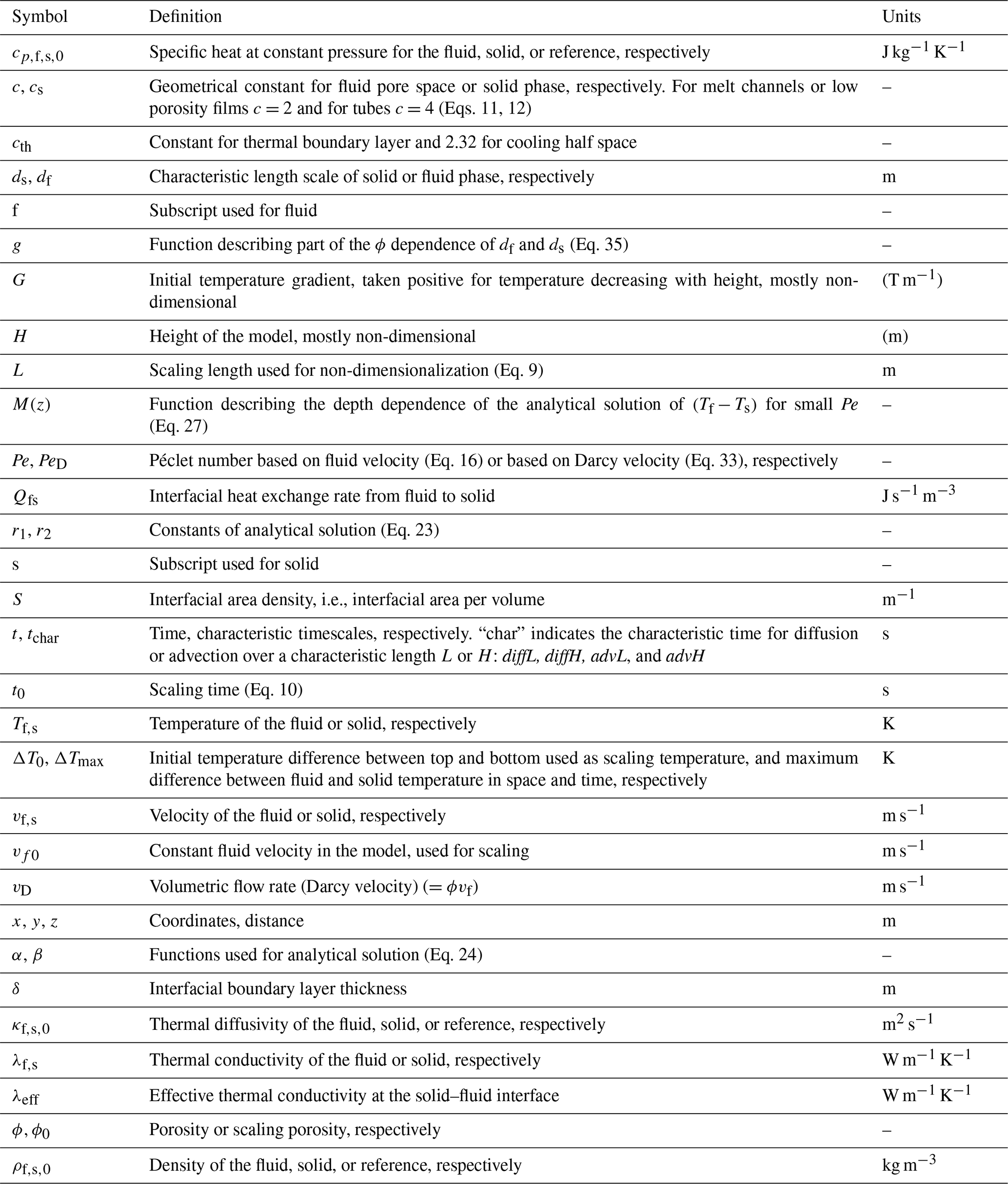
Table 1 Symbols, their definition, and physical units used in this study.

2.2 Scaling and non-dimensionalization

Non-dimensionalization is useful for interpreting models involving a large number of parameters. It usually helps reduce the number of parameters and identifies non-dimensional parameters that control the evolution of the system. We write the two energy conservation equations in a non-dimensional form, using

$$\begin{array}{}\text{(8)}& \begin{array}{rl}& T=\mathrm{\Delta }{T}_{\mathrm{0}}{T}^{\prime },t=t_{\mathrm{0}}{t}^{\prime },v=v_{\mathrm{f}\mathrm{0}}{v}^{\prime },\\ & \left(x,y,z\right)=L\cdot \left(x^{\prime },y^{\prime },z^{\prime }\right),\end{array}\end{array}$$

where ΔT₀ is the macroscopic scaling temperature difference of the system, i.e., the initial temperature difference between top and bottom; x,y, and z are distance; v_f0 is the scaling fluid velocity; L is the scaling length

$$\begin{array}{}\text{(9)}& L=\sqrt{{\displaystyle \frac{{\mathit{\varphi }}_{\mathrm{0}}\left(\mathrm{1}-{\mathit{\varphi }}_{\mathrm{0}}\right)\mathit{\delta }}{S}}},\end{array}$$

with ϕ₀ as a scaling porosity; and t₀ is the scaling time based on the diffusion time over the length L,

$$\begin{array}{}\text{(10)}& t_{\mathrm{0}}=L^{\mathrm{2}}/{\mathit{\kappa }}_{\mathrm{0}}\end{array}$$

(see Table 1 for definitions). Primed quantities are non-dimensional.

Introducing the fluid-filled pore width d_f and the solid width d_s, which may be the grain size or distance between fluid channels, the interfacial area density S scales with

$$\begin{array}{}\text{(11)}& S={\displaystyle \frac{c{\mathit{\varphi }}_{\mathrm{0}}}{d_{\mathrm{f}}}}\end{array}$$

for melt channels, tubes, pockets for all melt fractions, and melt films at small melt fractions, while S scales with

$$\begin{array}{}\text{(12)}& S={\displaystyle \frac{c_{\mathrm{s}}\left(\mathrm{1}-{\mathit{\varphi }}_{\mathrm{0}}\right)}{d_{\mathrm{s}}}}\end{array}$$

for melt channels, films, and suspensions at all melt fractions. Here c is a geometrical constant of the order of 2 for melt channels, 4 for melt tubes, 6 for melt pockets, and 2 for melt films at small melt fractions. It should be emphasized that Eqs. (11) and (12) are different ways of calculating the same S. The geometrical constant c_s is of the order of 2 for melt channels and 6 for melt films or suspensions. Thus, the scaling time and scaling length can also be written as

$$\begin{array}{}\text{(10a)}& t_{\mathrm{0}}={\displaystyle \frac{\left(\mathrm{1}-{\mathit{\varphi }}_{\mathrm{0}}\right)d_{\mathrm{f}}\mathit{\delta }}{c{\mathit{\kappa }}_{\mathrm{0}}}}={\displaystyle \frac{{\mathit{\varphi }}_{\mathrm{0}}{d}_{\mathrm{s}}\mathit{\delta }}{c_{\mathrm{s}}{\mathit{\kappa }}_{\mathrm{0}}}}\end{array}$$

and

$$\begin{array}{}\text{(9a)}& L=\sqrt{{\displaystyle \frac{\left(\mathrm{1}-{\mathit{\varphi }}_{\mathrm{0}}\right)\mathit{\delta }{d}_{\mathrm{f}}}{c}}}=\sqrt{{\displaystyle \frac{{\mathit{\varphi }}_{\mathrm{0}}\mathit{\delta }{d}_{\mathrm{s}}}{c_{\mathrm{s}}}}}.\end{array}$$

Equation (9a) shows that L scales both with the geometric mean of d_f and δ at small melt fractions and with the geometric mean of d_s and δ at large melt fractions. Thus, L is a natural length scale associated with thermal equilibrium of fluid-filled pores. The above scaling laws for S justify using the term ϕ₀(1−ϕ₀) in the scaling length L. It should be noted that we introduce and understand d_s as the average distance between melt-filled pores or channels, which can be considerably larger than the grain size. Then both δ and d_s and thus L can reach some considerable fraction of the system dimension.

We assume that the fluid and solid phases have the same densities and thermal properties (but relax this assumption later in Sect. 5.1.3):

$$\begin{array}{}\text{(13)}& \begin{array}{rl}& c_{p,\mathrm{f}}=c_{p,\mathrm{s}}=c_{p,\mathrm{0}},{\mathit{\rho }}_{\mathrm{f}}={\mathit{\rho }}_{\mathrm{s}}={\mathit{\rho }}_{\mathrm{0}},\\ & {\mathit{\kappa }}_{\mathrm{f}}={\mathit{\kappa }}_{\mathrm{s}}={\displaystyle \frac{{\mathit{\lambda }}_{\mathrm{eff}}}{c_{p,\mathrm{0}}{\mathit{\rho }}_{\mathrm{0}}}}={\mathit{\kappa }}_{\mathrm{0}}.\end{array}\end{array}$$

From Eqs. (4), (6), and (7) we get the non-dimensional energy conservation equations for the fluid and solid phases, respectively:

$$\begin{array}{}\text{(14)}& {\displaystyle }\begin{array}{rl}& \mathit{\varphi }\left({\displaystyle \frac{\partial T_{\mathrm{f}}^{\prime }}{\partial t^{\prime }}}+\mathit{Pe}{v}_{\mathrm{f}}^{\prime }\cdot \mathrm{\nabla }{T}_{\mathrm{f}}^{\prime }\right)\\ & =\mathrm{\nabla }\cdot \left(\mathit{\varphi }\mathrm{\nabla }{T}_{\mathrm{f}}^{\prime }\right)-{\mathit{\varphi }}_{\mathrm{0}}\left(\mathrm{1}-{\mathit{\varphi }}_{\mathrm{0}}\right)\left(T_{\mathrm{f}}^{\prime }-T_{\mathrm{s}}^{\prime }\right),\end{array}\text{(15)}& {\displaystyle }\begin{array}{rl}& \left(\mathrm{1}-\mathit{\varphi }\right){\displaystyle \frac{\partial T_{\mathrm{s}}^{\prime }}{\partial t^{\prime }}}\\ & =\mathrm{\nabla }\cdot \left(\left(\mathrm{1}-\mathit{\varphi }\right)\mathrm{\nabla }{T}_{\mathrm{s}}^{\prime }\right)+{\mathit{\varphi }}_{\mathrm{0}}\left(\mathrm{1}-{\mathit{\varphi }}_{\mathrm{0}}\right)\left(T_{\mathrm{f}}^{\prime }-T_{\mathrm{s}}^{\prime }\right).\end{array}\end{array}$$

From these equations we notice that the thermal evolution of the two-phase system is controlled by two non-dimensional numbers: the scaling porosity ϕ₀ and the Péclet number Pe defined as

$$\begin{array}{}\text{(16)}& \mathit{Pe}={\displaystyle \frac{v_{\mathrm{f}\mathrm{0}}L}{{\mathit{\kappa }}_{\mathrm{0}}}}.\end{array}$$

This number has already proven to be of high significance for determining whether thermal non-equilibrium is present or not (Schmeling et al., 2018), and the highest Pe corresponds to the largest temperature difference between fluid and matrix. In the following we drop the primes, keeping all equations non-dimensional, if not indicated otherwise.

In the following we consider a homogeneous two-phase matrix–fluid system in 1D with a porosity constant in space and time, i.e., ϕ=ϕ₀. We assume a constant fluid velocity which will be expressed in terms of Pe, thus we choose the non-dimensional velocity v_f=1. This simplifies Eqs. (14) and (15) to

$$\begin{array}{}\text{(17)}& {\displaystyle \frac{\partial T_{\mathrm{f}}}{\partial t}}+\mathit{Pe}{\displaystyle \frac{\partial T_{\mathrm{f}}}{\partial z}}={\displaystyle \frac{{\partial }^{\mathrm{2}}{T}_{\mathrm{f}}}{\partial z^{\mathrm{2}}}}-\left(\mathrm{1}-{\mathit{\varphi }}_{\mathrm{0}}\right)\left(T_{\mathrm{f}}-T_{\mathrm{s}}\right)\end{array}$$

and

$$\begin{array}{}\text{(18)}& {\displaystyle \frac{\partial T_{\mathrm{s}}}{\partial t}}={\displaystyle \frac{{\partial }^{\mathrm{2}}{T}_{\mathrm{s}}}{\partial z^{\mathrm{2}}}}+{\mathit{\varphi }}_{\mathrm{0}}\left(T_{\mathrm{f}}-T_{\mathrm{s}}\right),\end{array}$$

respectively. As we are interested in the evolution of the non-equilibrium temperature difference between the solid and fluid, subtraction of Eq. (18) from Eq. (17) gives

$$\begin{array}{}\text{(19)}& {\displaystyle \frac{\partial \left(T_{\mathrm{f}}-T_{\mathrm{s}}\right)}{\partial t}}-{\displaystyle \frac{{\partial }^{\mathrm{2}}\left(T_{\mathrm{f}}-T_{\mathrm{s}}\right)}{\partial z^{\mathrm{2}}}}+\mathit{Pe}{\displaystyle \frac{\partial T_{\mathrm{f}}}{\partial z}}+\left(T_{\mathrm{f}}-T_{\mathrm{s}}\right)=\mathrm{0},\end{array}$$

which is equivalent to

$$\begin{array}{}\text{(20)}& \begin{array}{rl}& {\displaystyle \frac{\partial \left(T_{\mathrm{f}}-T_{\mathrm{s}}\right)}{\partial t}}-{\displaystyle \frac{{\partial }^{\mathrm{2}}\left(T_{\mathrm{f}}-T_{\mathrm{s}}\right)}{\partial z^{\mathrm{2}}}}+\mathit{Pe}{\displaystyle \frac{\partial \left(T_{\mathrm{f}}-T_{\mathrm{s}}\right)}{\partial z}}+\left(T_{\mathrm{f}}-T_{\mathrm{s}}\right)\\ & =-\mathit{Pe}{\displaystyle \frac{\partial T_{\mathrm{s}}}{\partial z}}.\end{array}\end{array}$$

Note that while the temperatures T_f and T_s explicitly depend on two non-dimensional numbers Pe and ϕ₀, the temporal evolution of the temperature difference (T_f−T_s) explicitly depends only on Pe. However, implicitly it is still a function of ϕ₀ because T_s on the right-hand side of Eq. (20) depends on ϕ₀ via Eq. (18). Only for cases or stages with T_s independent of ϕ₀ as proposed in Sect. 4 is the temperature difference (T_f−T_s) a function of only one non-dimensional parameter, Pe, and not of ϕ₀.

2.3 Model setup

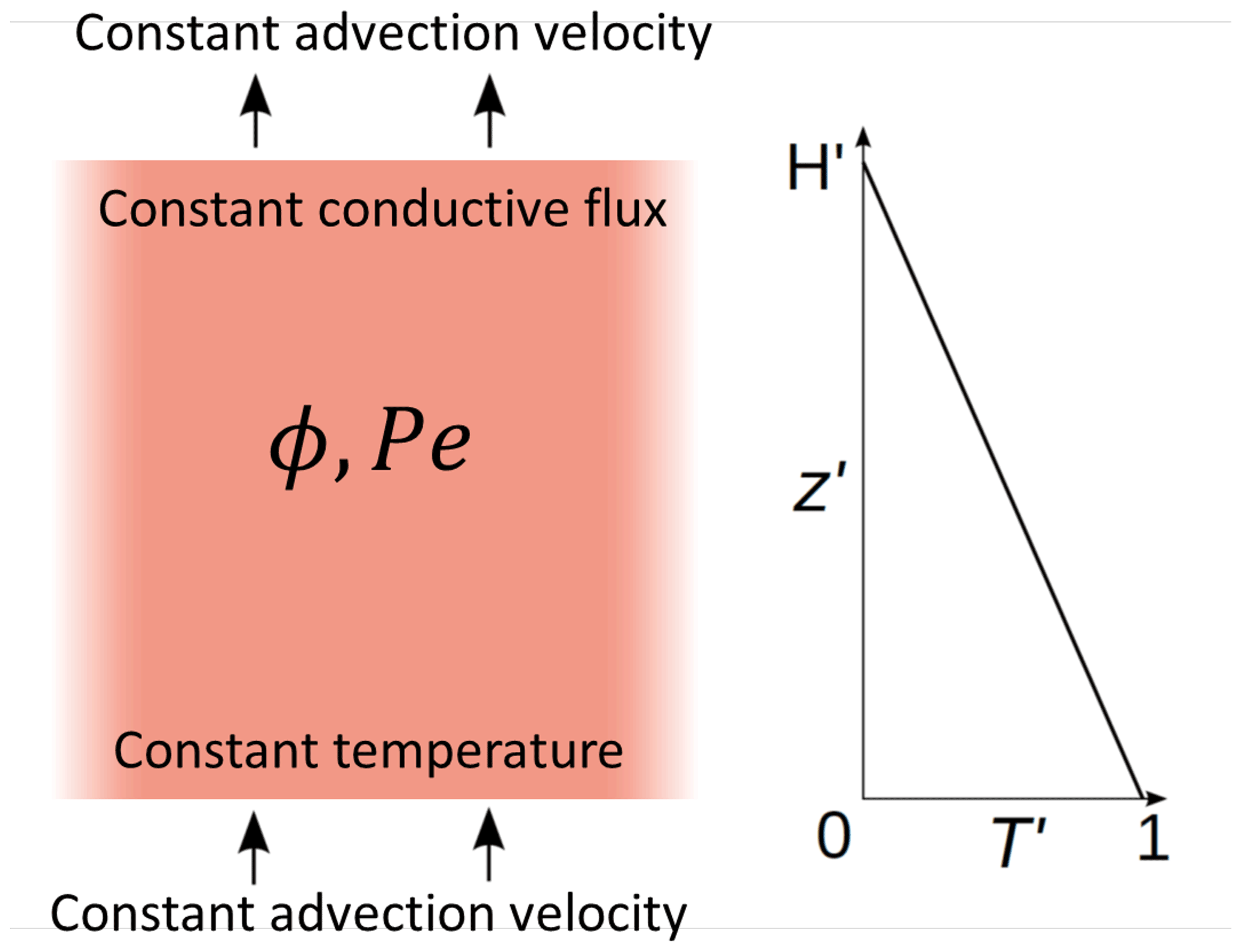
The fluid and solid heat conservation equations are solved in a 1D domain of height H. Other geometries could also be easily explored but are not considered here, since we focus on studying the relative control of the scaling parameters on thermal non-equilibrium evolution. At time t<0, both solid and fluid are at rest, in equilibrium. Both initial temperatures decrease linearly from 1 to 0 with z; therefore a constant temperature gradient of $-G=-\mathrm{1}/H$ is present in both phases (see Fig. 1). As a boundary condition both phase temperatures are set to 1 (non-dimensional temperature) at z=0. At z=H a constant thermal gradient condition $\partial T/\partial z=-\mathrm{1}/H$ (non-dimensional) is imposed for both phases. At z=0 the advective flux is fixed by the constant temperature condition (i.e., it is equal to Pe ϕ₀) while at z=H it evolves freely with the fluid temperature (i.e., it is given by T_fPeϕ₀, all non-dimensional). This top boundary condition needs some justification: the hyperbolic partial differential Eqs. (17) or (18) require two well-defined boundary conditions each, Dirichlet (fixed temperature), Neumann (fixed thermal gradient), Robin (linear combination of Neumann and Dirichlet), or Cauchy (fixed temperature and thermal gradient). Applying the Dirichlet condition at the bottom leaves either a Dirichlet, a Neumann, or a Robin condition to specify for the top. Different combinations of these boundary conditions can be applied separately for the fluid and the solid. For example, for the fluid a Neumann condition with zero or a small temperature gradient may be reasonable, while for the solid one may consider a Robin boundary condition mimicking a thick conductive lid with an internal constant temperature gradient and a fixed surface temperature. However, temporal changes of the temperature at the top (for our system, equal to the bottom of the lid) would lead to unphysical variations in the constant slope of the temperature gradient within the imagined lid. This is because the temperature in the lid can only vary on the diffusive timescale of the lid, which is much longer than all timescales in our model as long as the lid is thicker than H. In fact, in an open outflow situation like our system the evolution of the temperature, the thermal gradient, and the total (advective plus conductive) heat flux are not known a priori, but depend on the evolution within the system. In the early stage of model evolution, both the solid and fluid have a thermal gradient inherited from the initial condition, which is advected upwards in the fluid. Thus it seems most appropriate to use the Neumann condition as a boundary condition for both the solid and fluid. Only at later stages does this boundary condition impose artifacts in the temperature field close to the top boundary. The limitations of this top boundary condition are tested and discussed in Sect. 5.1.2.

Figure 1 Initial and boundary conditions.

This model setup adds a third non-dimensional scaling parameter to the system, namely $G=\mathrm{1}/H$. It defines the initial non-dimensional temperature gradient or conductive heat flux, positive for a flux directed upwards. To summarize, the temperatures depend on the non-dimensional parameters Pe, ϕ₀, and G.

2.4 Numerical scheme

The equations are solved by a MATLAB (MATLAB R2021b) code using a finite difference scheme central in space for the conduction terms, upwind for the advection term, and explicit in time. The spatial resolution is dz=0.1 or, for a few cases in Fig. 3 below, $min\left(\mathrm{0.1},H/\mathrm{100}\right)$ for H<10. The time step was chosen as $\mathrm{d}t=\frac{\mathrm{1}}{\mathrm{4}}min\left(\mathrm{d}z/\mathit{Pe},\mathrm{d}{z}^{\mathrm{2}}\right)$, i.e., taking the minimum of the Courant or diffusion criterion. Tests with higher spatial and temporal resolution have been carried out and did not change the results visibly. The global heat balance has also been checked: the maximum relative heat balance error can be defined as ${\left.{\mathit{\delta }}_q=\frac{q_{\mathrm{tot}}\left(z=\mathrm{0}\right)-q_{\mathrm{tot}}\left(z=H\right)-H\frac{\partial T_{\mathrm{mean}}}{\partial t}}{\left(q_{\mathrm{tot}}\left(z=\mathrm{0}\right)+q_{\mathrm{tot}}\left(z=H\right)\right)/\mathrm{2}}\right|}_{max}$ , where q_tot is the total non-dimensional vertical heat flux (conductive and advective) and T_mean is the mean temperature of the model. δ_q has an error on the order of 1 (due to the upwind scheme) with respect to the grid size dz; i.e., it is approximately equal to const ⋅ dz, where the constant is of the order of 0.2 (i.e., 2 %) for high Péclet numbers and drops to 0.1 (1 %) or 0.01 (0.1 %) for Pe≅1 or smaller, respectively.

3 Numerical model results

First, some example numerical results are shown in Fig. 2 to understand the physics and the typical behavior.

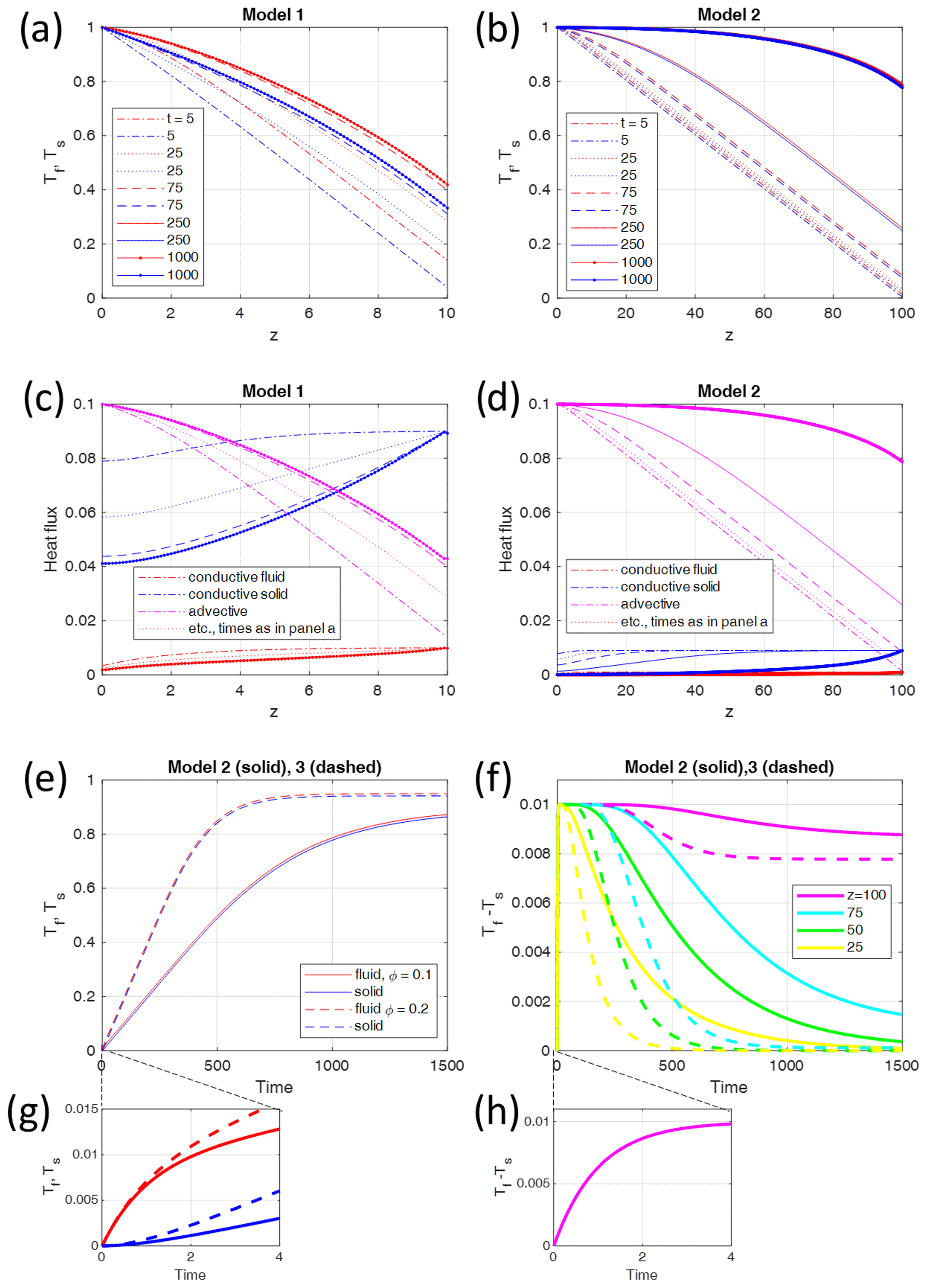
Figure 2 Typical model evolution for Pe=1, two different melt fractions ϕ, and two different non-dimensional temperature gradients G (i.e., heights H). (a) Model 1 is with G=0.1 (H=10) and ϕ=0.1. Red and blue curves show the fluid and solid temperatures at different non-dimensional times t as indicated by the legend, respectively. Initial temperatures are almost identical to the t=0.5 curves. Steady state is reached at about t=100; the curves of the last two times plot on each other. (b) Model 2 with G=0.01 (H=100), otherwise as in (a). Steady state is not fully reached. (c) Conductive (blue and red curves) and advective (magenta curve) heat fluxes through the solid and fluid, respectively, of model 1. Line styles indicate the same times as in (a). (d) Same as (c) but for model 2. (e) Temporal evolution of fluid and solid temperatures, T_f (red) and T_s (blue), respectively, at the top of model 2 with ϕ=0.1 and model 3 with ϕ=0.2. G=0.01 (H=100) for both models. (f) Evolution of fluid–solid temperature difference (T_f−T_s) at different distances z in model 2 (ϕ=0.1, solid curves) and in model 3 (ϕ=0.2, dashed curves). (g) Zoomed-in early temporal evolution of solid and fluid temperatures of models 2 and 3 shown in (e). (h) Zoomed-in early temporal evolution of temperature difference of models 2 and 3 shown in (f).

3.1 Evolution of temperatures and thermal non-equilibrium with time

Three different models have been run, all with Pe=1 and the following other parameters:

• model 1 – G=0.1 (H=10), ϕ=0.1,

• model 2 – G=0.01 (H=100), ϕ=0.1, and

• model 3 – G=0.01 (H=100), ϕ=0.2.

Figure 2a and b show T_f and T_s as functions of z at different times as indicated for two initial temperature gradients, G=0.1 (H=10) and G=0.01 (H=100). Figure 2c shows the different contributions to the depth-dependent conductive and advective heat fluxes through the solid and fluid phases, respectively. Figure 2e shows the evolution of T_f and T_s with time at the top of the domain, for the same model 2 as in Fig. 2b and for model 3 with a higher melt fraction ϕ=0.2. Figure 2f shows the evolution of (T_f−T_s) at different distances z of model 2 (ϕ=0.1) and of model 3 (ϕ=0.2). At each depth of the system, the fluid and solid temperatures, as well as the temperature difference and the heat fluxes, evolve following three stages.

Stage 1. During this transient stage the fluid temperature increases faster than the solid temperature (Fig. 2a, b, e, f), and the temperature difference (Fig. 2f, h) increases. During this stage, the fluid temperature increases rapidly at first, and then the temperature increase slows down. The conductive heat fluxes in both solid and fluid decrease rapidly and more slowly later, while the advective heat flux rapidly increases. As for the solid temperature, it first increases slowly and then faster and faster. At t=0, the fluid velocity is suddenly set to non-zero; thus the fluid temperature starts to deviate from equilibrium and increases due to these new conditions. If the solid temperature were maintained constant with time, the fluid temperature would probably reach a steady-state profile, depending on boundary conditions, fluid velocity, and solid temperature. While the fluid temperature increases faster than the solid temperature, the fluid–solid temperature difference, and thus the heat transfer term, increases too, forcing the solid temperature to progressively increase. At the end of stage 1 the maximum temperature difference is approached (Fig. 2h). Because the solid temperature has not risen significantly at that time (at t=4 in the example) compared to the fluid temperature (Fig. 2g), different melt fractions do not affect the temperature differences during this stage (Fig. 2h in which all curves merge into one curve). This observation confirms the expectation from Eq. (20) that the temperature difference does not depend on melt fraction as long as the solid temperature is independent of ϕ, which is the case as long as T_s stays close to its initial profile.

Stage 2. The fluid and the solid temperatures increase at similar rates, constant with time (Fig. 2e), and the temperature difference remains constant and at a maximum at the top (Fig. 2f). Solid–fluid heat transfer is at a maximum during this stage. As T_s is no longer constant in time, different melt fractions lead to different rates of temperature increase (Fig. 2e) and also to different evolutions of (T_f–T_s) (Fig. 2f solid curves compared to dashed curves). At higher melt fraction the heat transfer into the solid increases (see last term in Eq. 18), resulting in a faster increase in the solid temperature whose gradient flattens earlier. Thus, the end of stage 2 is reached earlier (Fig. 2e).

Stage 3. As the fluid temperature rises closer to the T_f value at the bottom, its increase slows down, and heat transfer, and thus temperature difference, decreases. In model 1 (Fig. 2a), steady state is reached while the fluid and solid temperatures are still far from 1. This is due to the influence of boundary conditions, as the heat transferred from the fluid phase to the solid phase is compensated for by the solid phase heat loss at the top of the domain. In model 2 (Fig. 2b), boundary conditions at z=H are applied farther away from the bottom, therefore allowing for a higher increase in temperatures when reaching the steady state.

At each z we observe that the temperature difference first increases rapidly to reach a maximum after a short time (stage 1), hereafter t=4 (Fig. 2h). The resulting amplitude of the temperature difference is identical at the different z positions and for both melt fractions. Then it stays constant at this maximum value (stage 2) and finally decreases (stage 3) (Fig. 2f). The higher in the model, the longer the temperature difference remains at maximum. A higher melt fraction accelerates the decrease in (T_f−T_s).

The absolute maximum temperature difference in space and time does not depend on boundary conditions (see also Sect. 5.1.2 where the influence of boundary conditions is discussed) or on the z position or on the melt fraction and therefore looks to be an interesting observable. It could indeed be useful for getting a first-order estimate of thermal non-equilibrium conditions and possible temperature differences in a magmatic system. In the following sections we study how this maximum temperature difference evolves when varying the parameter Pe.

Comparing the heat fluxes of model 1 (G=0.1) with those of model 2 (G=0.01) shows the importance of heat advection by the fluid phase: in model 1 (Fig. 2c) the conductive contribution through the solid is of the same order of magnitude as the advective contribution by the fluid because the initial temperature gradient G and the porosity φ are the same (=0.1). In model 2 (Fig. 2d), in spite of the same Péclet number, the smaller initial temperature gradient (G=0.01) reduced the conductive contribution with respect to the advective contribution by a factor of about 10, and advection dominates. Furthermore, the two models demonstrate that the conductive heat flux contributions may be important with respect to advective and interphase heat flux for sufficiently large initial thermal gradient (here 0.1), while it has been neglected in several earlier investigations (e.g., Schumann, 1929; Spiga and Spiga, 1981).

3.2 Maximum temperature difference

The maximum temperature difference of a model can be defined as the maximum value reached in space and time (see Fig. 2f). A series of models have been carried out for the two different non-dimensional parameters Pe and $G=\mathrm{1}/H$, and ΔT_max has been determined for each model (Fig. 3). Some first observations can be made.

• For all Pe values, ΔT_max is proportional to Pe (Fig. 3a) as long as ΔT_max is somewhat smaller than the absolutely possible maximum 1, which is asymptotically approached for high Pe.

• ΔT_max is proportional to G, i.e., to the non-dimensional temperature gradient for G<0.1.

• ΔT_max reaches a maximum for large G of the order of 1, i.e., when H reaches 1 or the dimensional H reaches the length scale L.

• ΔT_max is essentially independent of ϕ as models with different ϕ values almost merge in the same points shown in Fig. 3. This has been verified by running all models of Fig. 3 with melt fractions between 0.1 and 0.9 (not shown).

These observations suggest the existence of several domains in which scaling laws for ΔT_max could be derived, based on the two scaling parameters. In the next section, we propose an analytical derivation of ΔT_max values to obtain scaling laws and confirm the observed proportionalities.

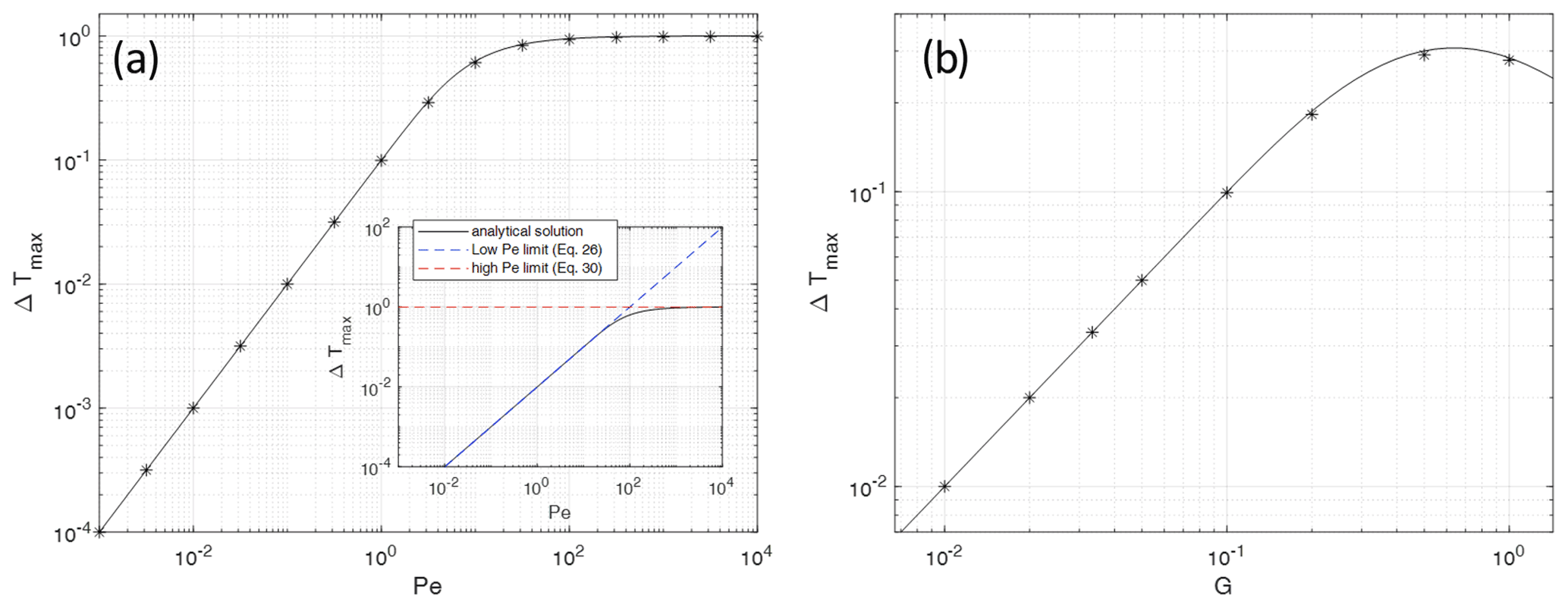
Figure 3 Maximum fluid–solid temperature differences T_f−T_s of numerical models (asterisks) with different parameters, plotted (a) as a function of the Péclet number Pe for G=0.1 and ϕ=0.1 and (b) as a function of the initial thermal gradient G for Pe=1 and ϕ=0.1. The solid lines give the analytic solutions. The inset in (a) shows the comparison of the analytic solution Eq. (22) with the different limits derived in Sect. 2.1 and 2.2. The black curve represents the analytic solution, and the colored straight lines show the results in the high or low value limits of Eqs. (26) to (30), respectively. A larger version of the inset is given as Fig. S1 in the Supplement. The analytical solution for the full parameter range Pe–G is given in Fig. 4.

4 Scaling laws derived from analytical solution

In this section a simplified analytical solution for the z-dependent temperature difference between fluid and solid will be derived. From this solution the maximum temperature differences ΔT_max can be obtained, and scaling laws will be derived.

4.1 Analytical solution of the governing equations

We are interested in an analytical solution of Eq. (20) controlling the non-equilibrium temperature difference (T_f−T_s). We simplify the problem by considering the hypothetical case in which (T_f−T_s) does not change with time and, moreover, in which the thermal gradient in the solid phase is fixed and linear, with $\partial T_{\mathrm{s}}/\partial z=-G=-\mathrm{1}/H$ (non-dimensional, with dimensions $G=\mathrm{\Delta }{T}_{\mathrm{0}}/H)$. Although different from initial and steady-state stages described in the 1D models (Sect. 3.1), this hypothetical case is quite similar to what can be observed at the very beginning of the second stage described in Sect. 3.1 (see Fig. 2f, h). In this second stage, the evolution of T_f and T_s was observed to be quite similar indeed. Besides, at the end of stage 1 (Sect. 3.1), T_s remains close to initial conditions; therefore a fixed linear gradient of slope $-G=-\mathrm{1}/H$ is justified. Since the maximum temperature difference between the two phases is observed starting from the end of stage 1 and during stage 2 (Sect. 3.2), it does not seem unreasonable to consider this hypothetical case for deriving the maximum temperature difference. Using these assumptions, Eq. (20) becomes

$$\begin{array}{}\text{(21)}& {\displaystyle \frac{{\partial }^{\mathrm{2}}\left(T_{\mathrm{f}}-T_{\mathrm{s}}\right)}{\partial z^{\mathrm{2}}}}-\mathit{Pe}{\displaystyle \frac{\partial \left(T_{\mathrm{f}}-T_{\mathrm{s}}\right)}{\partial z}}-\left(T_{\mathrm{f}}-T_{\mathrm{s}}\right)=-\mathit{Pe}G.\end{array}$$

While in the general case of Eq. (20) the temperature difference implicitly depends on ϕ₀, i.e., on the three non-dimensional parameters Pe, ϕ₀, and G, Eq. (21) no longer depends on ϕ₀ because we replaced $\partial T_{\mathrm{s}}\left({\mathit{\varphi }}_{\mathrm{0}}\right)/\partial z$ with −G, which is independent of ϕ₀. Equation (21) is a second-order ordinary differential equation for (T_f−T_s) whose solution can be analytically derived as (see Supplement for details)

$$\begin{array}{}\text{(22)}& T_{\mathrm{f}}-T_{\mathrm{s}}=\mathit{\alpha }{e}^{r_{\mathrm{1}}z}+\mathit{\beta }{e}^{r_{\mathrm{2}}z}+\mathit{Pe}G,\end{array}$$

where r₁ and r₂ are the roots of the associated equation of Eq. (21):

$$\begin{array}{}\text{(23)}& r_{\mathrm{1}}={\displaystyle \frac{\mathrm{1}}{\mathrm{2}}}\left(\mathit{Pe}-\sqrt{{\mathit{Pe}}^{\mathrm{2}}+\mathrm{4}}\right),r_{\mathrm{2}}={\displaystyle \frac{\mathrm{1}}{\mathrm{2}}}\left(\mathit{Pe}+\sqrt{{\mathit{Pe}}^{\mathrm{2}}+\mathrm{4}}\right).\end{array}$$

The parameters α and β are constrained by the boundary conditions $\left(T_{\mathrm{f}}-T_{\mathrm{s}}\right)=\mathrm{0}$ at z= 0 and $\frac{\partial \left(T_{\mathrm{f}}-T_{\mathrm{s}}\right)}{\partial z}=\mathrm{0}$ at z=H:

$$\begin{array}{}\text{(24)}& \begin{array}{rl}& \mathit{\alpha }=\mathit{Pe}G{\displaystyle \frac{r_{\mathrm{2}}}{r_{\mathrm{1}}{e}^{\left(r_{\mathrm{1}}-r_{\mathrm{2}}\right)/G}-r_{\mathrm{2}}}},\\ & \mathit{\beta }=\mathit{Pe}G{\displaystyle \frac{r_{\mathrm{1}}}{r_{\mathrm{2}}{e}^{\left(r_{\mathrm{2}}-r_{\mathrm{1}}\right)/G}-r_{\mathrm{1}}}}.\end{array}\end{array}$$

The third term in Eq. (22) is a particular solution for Eq. (21).

4.2 Comparison with numerical models

From Eq. (22) the maximum value of the depth-dependent temperature difference (T_f−T_s) can be determined. It is found that the maximum is always at z=H. This value will be denoted as ΔT_max and has been calculated for all parameter combinations used for the numerical models. In Fig. 3 these analytical solutions are plotted as solid lines together with the numerical solutions (asterisks). The agreement is very good. For most cases the differences between the numerical and analytical solutions are well below 1 %; only when ΔT_max reaches values of about 0.6 and higher do the differences become >1 %, up to 6 %. This general good agreement is another justification for using the time-independent Eq. (21) to obtain an analytical solution of an intrinsically time-dependent process as long as we are interested only in the maximum value of (T_f−T_s). Other reasons for the observed differences between the analytical and numerical solutions include numerical errors when determining the particular times when maximum temperature differences are reached, especially for the models which are in the regime close to $\mathrm{\Delta }{T}_{max}=\mathrm{1}$ where the ΔT_max(Pe) curves become non-linear (Fig. 3a).

4.3 Scaling laws for temperature differences at certain parameter limits

The analytical solution for ΔT_max fits very well with our model results and therefore looks to be ideal for getting a better understanding of the relative influences of the two controlling parameters Pe and G, described in Sect. 2.2 and 2.3. The Péclet number is already known to be of great importance for thermal equilibrium and non-equilibrium conditions. Inspecting the last term in Eq. (22) we notice that a high Pe and a high initial thermal gradient should favor higher temperature differences. This has been demonstrated in Fig. 3.

Equation (22) is, however, complicated, and the assessment of the relative importance of Pe and G for different possible regimes is limited. In this section, we study the evolution of (T_f−T_s), i.e., also ΔT_max, in a few limiting cases. This enables us to better understand the influence of each parameter and to derive some scaling laws for different regimes.

4.3.1 Limit Pe→0

When Pe tends to 0, we have the condition

$$\begin{array}{}\text{(25)}& \mathit{Pe}\ll \mathrm{2}.\end{array}$$

With this condition Eq. (22) tends to the following limit (see Supplement):

$$\begin{array}{}\text{(26)}& T_{\mathrm{f}}-T_{\mathrm{s}}=\mathit{Pe}G\left(\mathrm{1}-M\right),\end{array}$$

with

$$\begin{array}{}\text{(27)}& M={\displaystyle \frac{\cosh \left(z\right)+\cosh \left(\frac{\mathrm{2}}{G}-z\right)}{\mathrm{1}+\cosh (\mathrm{2}/G)}},\end{array}$$

which simplifies for $z=H=\mathrm{1}/G$ to

$$\begin{array}{}\text{(28)}& M={\displaystyle \frac{\mathrm{1}}{\cosh (\mathrm{1}/G)}}.\end{array}$$

This is the limit for Pe→0. This limit gives predictions for ΔT_max in very good agreement with Eq. (22) for Pe<1 (having G=0.1) (see inset in Fig. 3a or Fig. S1 in the Supplement). In the limit G→0 and finite $\mathit{Pe}<\mathrm{1}/G$ we get the limit for M

$$M\to e^{-z}.$$

Thus, for both small Pe and small G the temperature difference (Eq. 26) can be written as

$$\begin{array}{}\text{(29)}& T_{\mathrm{f}}-T_{\mathrm{s}}=\mathit{Pe}G\left(\mathrm{1}-e^{-z}\right).\end{array}$$

Equation (29) confirms the proportionalities observed in Fig. 3, namely $\mathrm{\Delta }{T}_{max}\propto \mathit{Pe}$ (Fig. 3a) and $\mathrm{\Delta }{T}_{max}\propto G$ (Fig. 1b).

4.3.2 Limit Pe→∞

To obtain the limit of Eq. (22) for Pe→∞, Eq. (22) can be linearized with respect to $\mathrm{4}/{\mathit{Pe}}^{\mathrm{2}}\ll \mathrm{1}$. Applying the rule of L'Hôpital, Eq. (22) tends to the following limit:

$$\begin{array}{}\text{(30)}& T_{\mathrm{f}}-T_{\mathrm{s}}=Gz.\end{array}$$

For details, see the Supplement. This limit is also the solution of Eq. (21) when neglecting the diffusive and heat transfer terms. As demonstrated in the Supplement, this limit predicts ΔT_max values in very good agreement with Eq. (22) for Pe>100 (Fig. 3a, inset).

4.3.3 Exploring the domains for the maximum temperature difference including all limits

Before exploring the full parameter space, we first give a short overview of expected parameter ranges in magmatic systems.

In natural magmatic systems such as mid-ocean ridges, Pe is expected to evolve from very low values of the order of 10⁻⁵ to 10⁻³ in partially molten regions with distributed porous flow to higher values of the order of 1 or larger at depths where channels have merged and further to very high values of the order of 10⁵ in dike systems (Schmeling et al., 2018).

While the melt fraction does not influence ΔT_max (cf. Eqs. 22, 30), it does influence the long-term temporal behavior because T_s is ϕ₀-dependent (see Eq. 20). Therefore, here follow some words about possible melt fractions. As melt flow may occur at very small melt fractions (McKenzie, 2000; Landwehr et al., 2001), large ϕ values are not expected in natural mantle magmatic systems or in dike systems in the crust. Values of channel volume fraction generally remain below a few percent up to tens of percent (in dunite channels up to 10 %–20 %, Kelemen et al., 1997).

To get an idea about the expected order of magnitude of the macroscopic thermal gradient $G=\mathrm{1}/H$ of the system, we have to evaluate the scaling length L used to scale the dimensional H. L scales with the geometric mean of the channel width d_f and the interfacial boundary layer thickness δ (Eqs. 9 with 11). L would evolve non-linearly with the width of melt pathways, which may increase by several orders of magnitude as 3D grain junctions eventually merge to 1D dikes. As will be shown in Sect. 5.3 in more detail the resulting non-dimensional G ranges between an order of 1 and an order of 10⁻⁵.

In Fig. 4 we explore ΔT_max variations using the analytical solution Eq. (22), in which ΔT_max depends on Pe and G. Three main regimes can be distinguished.

• Regime 1. For high Pe values, (T_f−T_s) tends to the relationship described in Eq. (30). The temperature difference increases linearly with distance from the bottom (z=0), reaching $\mathrm{\Delta }{T}_{max}=\mathrm{1}$ at z=H. In the whole region the fluid temperature remains constant and at a maximum of 1 while the solid temperature increases linearly with z from 0 to 1. The proportionality of ΔT_max to G disappears because the maximum value of z is equal to $H=\mathrm{1}/G$.

• Regime 2. For Pe≪1, or more precisely, for $\mathit{Pe}\ll \frac{\mathrm{1}}{G}$ represented by the oblique dashed line in Fig. 4, (T_f−T_s) varies with distance from the bottom according to $\left(\mathrm{1}-e^{-z}\right)$ and is proportional to Pe and G. This means that large temperature gradients favor large temperature differences. In this domain, (T_f−T_s) tends to the relationship presented in Eq. (29).

• Regime 3. For a large initial temperature gradient G close to 1 (small H) and Pe≪1, (T_f−T_s) tends to the relationship proposed in Eq. (26). In this domain, (T_f−T_s) is proportional to Pe but no more to G because M is a function of G gradually canceling the proportionality to G, which is visible in regime 2. The depth dependence is given by (1−M(z)), which at G=1 increases non-linearly from about 0 to 0.4 with increasing z.

Figure 4 Main regimes of the maximum fluid–solid temperature differences ΔT_max due to thermal non-equilibrium obtained by the analytical solution (Eq. 22) in the parameter space of the Péclet number Pe and temperature gradient G. The asymptotic limits are indicated by the formulas, and M(z) is given by Eq. (27) with $\left(\mathrm{1}-M\left(G,z\right)\right)$ increasing non-linearly from about 0 to about 0.4 with increasing z for G in the range 0.3 to 3. Regime boundaries are shown as dashed lines. Typical parameter combinations for magmatic settings such as interstitial melts or dikes are indicated by the orange rectangles which extend further to the left, well below log ₁₀G of −3. Note that two slices through this field at G=0.1 and at Pe=1 have already been shown in Fig. 3.

5 Discussion

5.1 Limitations

5.1.1 Comments on the analytic solution

Although the assumptions used to get the analytic solution (Eq. 22) are very specific, they are reasonable considering the conditions in the models when ΔT_max is reached, and it fits the numerical results very well. This is shown in Fig. 5 where for various combinations of Pe and G the time-dependent temperature differences (T_f−T_s) are shown as functions of depth together with the analytical solutions using Eq. (22). For all examples the position of the maximum temperature differences lies at z=H. A major simplification used in Eq. (21) was time independence. Obviously, the resulting analytical solutions represent stage 2, which is quasi steady state in contrast to stage 1 when the temperature difference builds up and stage 3 when the long-term behavior is approached. We emphasize that this analytical solution is a very good approximation of the depth-dependent temporal maximum temperature difference that can be reached in such porous systems.

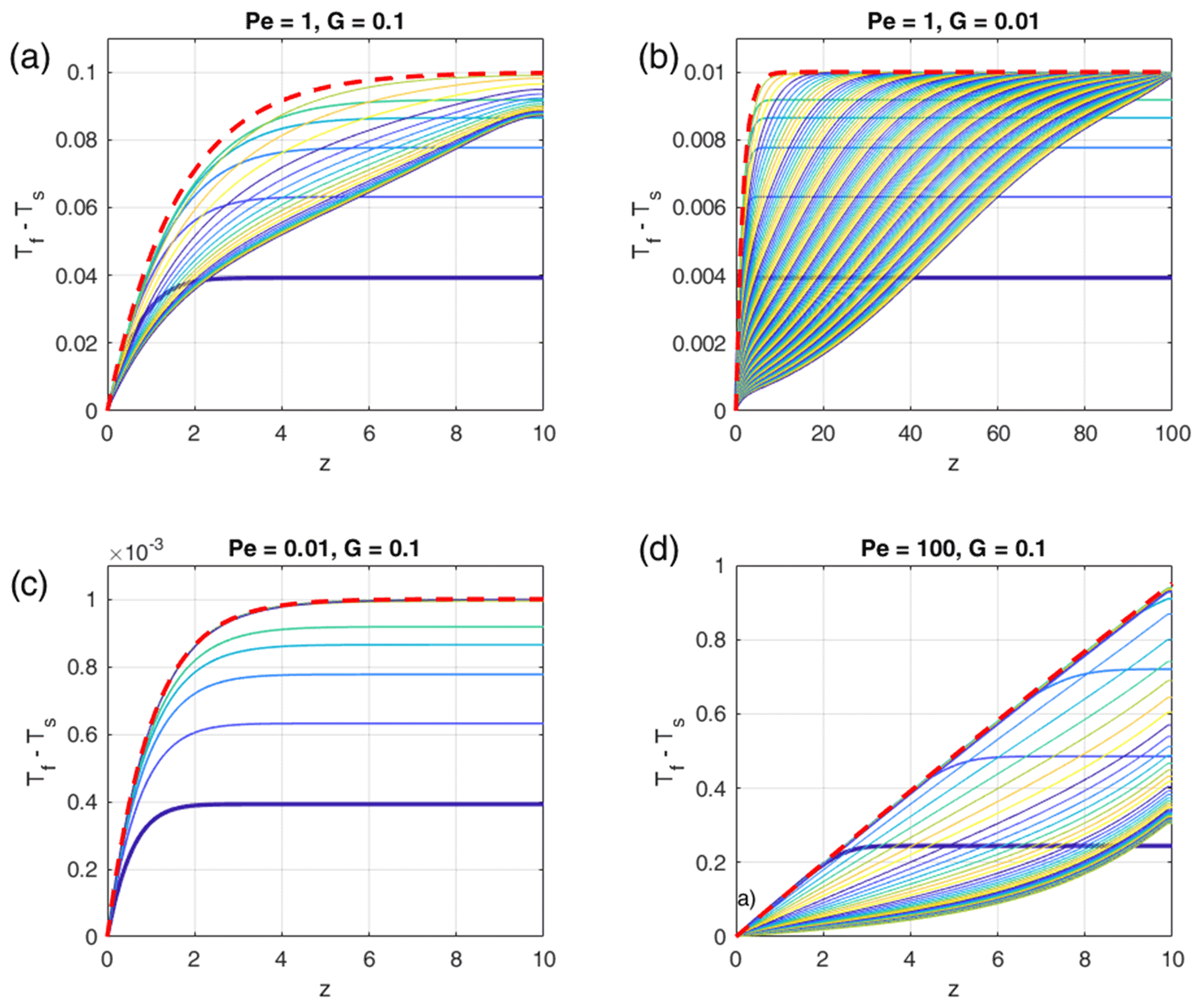
Figure 5 Comparison of depth- and time-dependent numerical solutions with the time-independent analytical solutions for different parameters Pe and G as indicated in the panel titles. In each panel the curves show (T_f−T_s) profiles for progressive times, and the colors are cyclically varied with time from blue to yellow, starting with blue (bold curve). The bold red dashed curve shows the analytical solution Eq. (22), which represents a very good estimate of the depth-dependent temporal maximum of the temperature difference. In each panel the first five curves are plotted at time increments of 0.5 (0.025 for Pe=100) and the later curves with 5 (1 for Pe=100). The total non-dimensional times of each panel are 100 (500 for G=0.01). Steady state is reached in the models with G=0.1. The model with G=0.01 would need t = 10 000 to reach steady state. The melt fraction was chosen as ϕ₀=0.1.

5.1.2 Boundary conditions at top and initial conditions

The boundary conditions we chose at the top (z=H) are suitable for cases with little temperature evolution (regimes 2 and 3, low Pe) and for early stages for regime 1 but might be inappropriate for high temperature increases (high Pe – regime 1) at later stages (see Sect. 4.3.4). In order to quantify the influence of this choice of boundary conditions on our results, we compared the evolution of (T_f−T_s) profiles for three Péclet numbers and two values of G, using four different boundary conditions at the top (Fig. 6).

• Constant thermal gradient equal to the initial thermal gradient in the solid and fluid phases (Neumann condition). This was the boundary condition used in the models.

• The thermal gradient is set to 0 at the top (Neumann condition).

• Both fluid and solid temperatures are set to 0 at the top (Dirichlet condition).

• Temperature at the top is numerically calculated from the full Eqs. (17) and (18) using one-sided (upwind) positions for the first and second derivatives (open boundary).

Mathematically, the open boundary condition is not a rigorous boundary condition because both the temperature and temperature gradient intrinsically depend on the temperature evolution within the model. Therefore, it cannot be applied to the analytical solution of Sect. 4.1. Numerically it works well for our system without producing instabilities or oscillations. Comparing the top and bottom rows of Fig. 6, the constant temperature gradient condition produces quite similar results as the open boundary condition for all Pe and G values tested during the first and second stages of temporal evolution (see Sect. 3.1). The agreement becomes worse for stage 3 when approaching steady state at large Pe values. Comparing the other two boundary conditions (second and third rows of Fig. 6) with the constant gradient condition (top row) shows that the effect of the top boundary during stages 1 and 2 is still small sufficiently far away from the top. Only for the small Pe case (left column of Fig. 6) do the zero gradient and zero temperature conditions strongly affect the upper half of the domain by diffusion. Yet the maximum temperature difference of the constant gradient case is nearly reached by the other two boundary conditions further within the domain, not at the top. The special case of high Pe and small G with zero temperature boundary condition (third row, fourth column in Fig. 6) shows a strong build-up of T_f−T_s close to the top when approaching the steady state. This stems from the large local temperature gradient built up near the top as a result of transforming the difference in advective heat in- and output $\left(\mathit{Pe}{T}_{\mathrm{influx}}-\mathit{Pe}{T}_{\mathrm{outflux}}=\mathit{Pe}\right)$ into a high conductive outflux $\left(\partial T/\partial z\right)$ at the top. It is unlikely that such situations occur in natural systems.

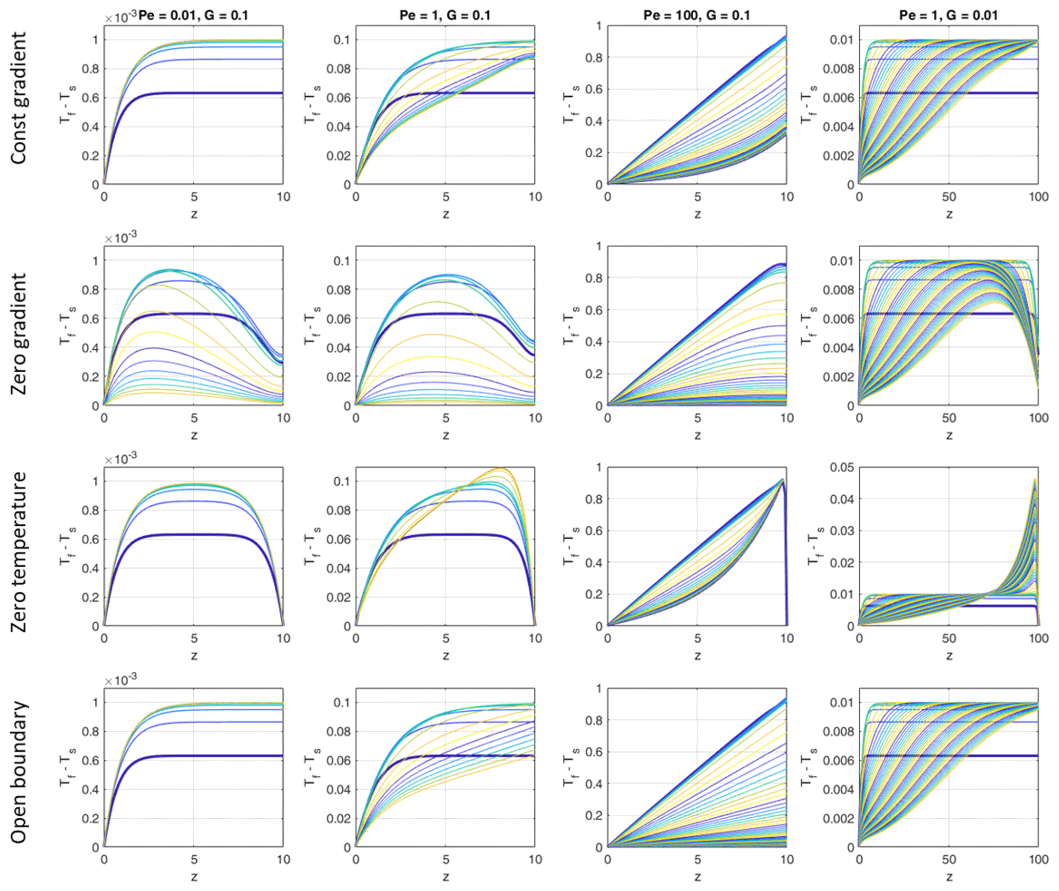
Figure 6 Temporal evolution of vertical profiles of (T_f−T_s) for models with different Péclet numbers and different initial temperature gradients G. In each panel the curves show (T_f−T_s) profiles for progressive times, and the colors are cyclically varied with time from blue to yellow, starting with blue (bold curve). The first five curves of the Pe<100 (respectively Pe=100) models were taken with time increments of 1 (respectively 0.1) and the later curves with 10 (respectively 1). The total time was 100 in all models with G=0.1 and 500 in the models with G=0.01. Steady state is reached in the models with G=0.1. The models with G=0.01 would need t = 10 000 to reach steady state. In each row the top boundary conditions are assumed as indicated at the left.

We have also tested an open boundary condition for the fluid and a Robin boundary condition for the solid imagining a lid on top of our model with a constant temperature gradient and a fixed surface temperature. Choosing the surface temperature in such a way that the initial thermal gradient within our system and within the lid are identical, this boundary condition adds a new non-dimensional parameter, the lid thickness H_lid. Tests show that lid thicknesses larger than H give results in general agreement with the constant gradient or open boundary models of Fig. 6. Localized differences with up to 30 % higher (T_f−T_s) values occur near the top, but they disappear for H_lid≥10 H. Lid thicknesses smaller than H force the solid temperature at the top to values closer to 0, while the fluid temperature remains high. This results in significantly higher (T_f−T_s) values than in Fig. 6 (top row) close to the top. However, typical natural magmatic systems are on the H_lid>H side, suggesting that our constant gradient boundary condition is a good approximation.

In summary, the influence of boundary conditions on fluid and solid temperature evolution depends mostly on the domain size H and on the value of Pe. The larger these two parameters, the less important the influence of boundary conditions within almost the whole model domain. If one is interested in the maximum value of T_f−T_s in space and time, the tests show that this value can safely be picked at z=H when using the constant temperature gradient boundary condition.

As an initial condition we used a linear temperature profile and initial equilibrium between solid and fluid. A non-linear initial temperature profile between $T_{\mathrm{f}}=T_{\mathrm{s}}=\mathrm{1}$ at the bottom and $T_{\mathrm{f}}=T_{\mathrm{s}}=\mathrm{0}$ at the top would have spatially varying temperature gradients with sections with gradients larger than those assumed in our model. As the temperature gradient strongly influences thermal non-equilibrium (see e.g., Eq. 22, which explicitly contains the temperature gradient G), the above results are expected to be different, and a stronger thermal non-equilibrium is expected in regions with higher gradients. Schmeling et al. (2018) used a step function with $T_{\mathrm{f}}=T_{\mathrm{s}}=\mathrm{1}$ at z=0 and $T_{\mathrm{f}}=T_{\mathrm{s}}=\mathrm{0}$ at z>0 as the initial condition, i.e., an extremely non-linear profile near z=0. Assuming this initial temperature profile, Fig. 7 shows the temporal behavior of the temperature difference for selected parameter combinations, equal to the parameters used in Fig. 5. The analytical solutions for the time-independent cases (Eq. 22) are also shown. As expected, at early stages the temperature differences are significantly larger than given by the analytical solutions by a factor of 2 or more shortly after the onset of the evolution. At later stages (stage 2 or 3) the time-dependent solutions approach or pass through the analytical solutions. Thus, we may state that the analytical solutions depicted in the regime diagram in Fig. 4 represent lower bounds of thermal non-equilibrium compared to settings with non-linear initial temperature profiles.

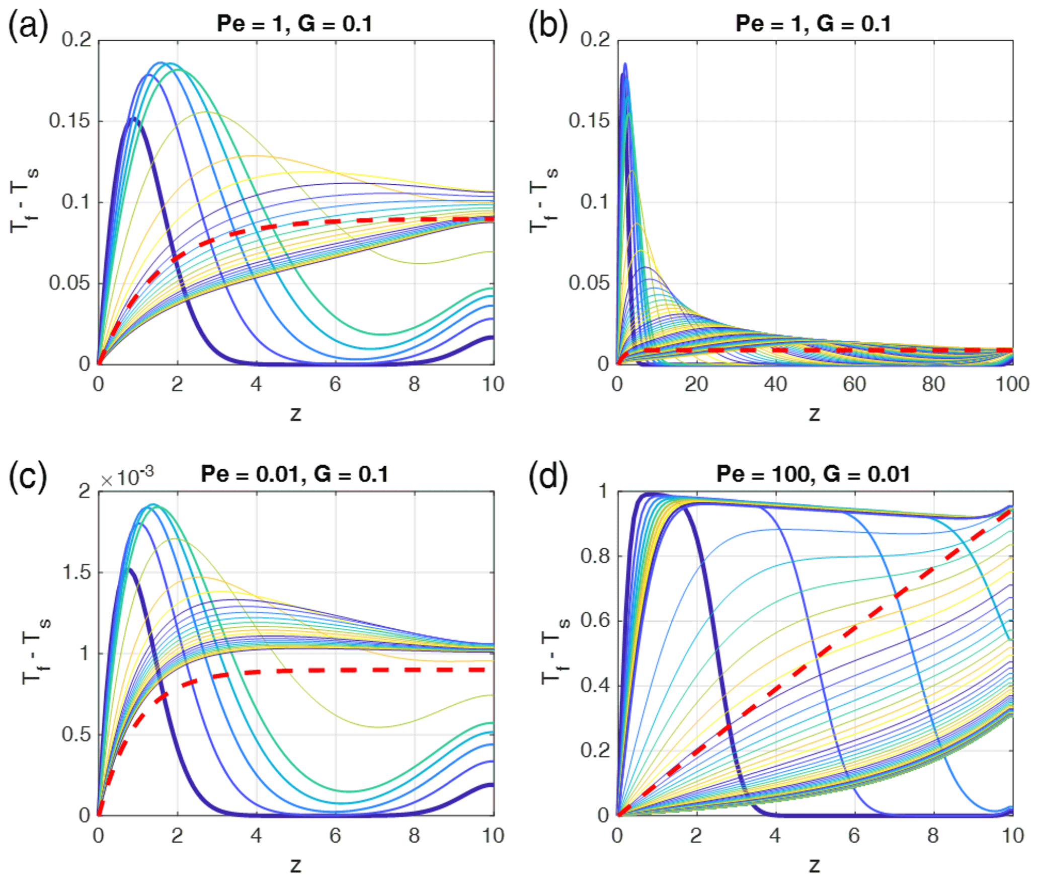
Figure 7 Time- and depth-dependent numerical solutions (thin curves) as in Fig. 5 but for step-function initial conditions: $T_{\mathrm{f}}=T_{\mathrm{s}}=\mathrm{1}$ at z=0 and $T_{\mathrm{f}}=T_{\mathrm{s}}=\mathrm{0}$ at z>0 at t=0. The bold dashed red curves are the time-independent analytical solutions as in Fig. 5. In each panel the curves show (T_f−T_s) profiles for progressive times, and the colors are cyclically varied with time from blue to yellow, starting with blue (bold curve). In each panel the first five curves (and later curves, respectively) are plotted at time increments of (a) 0.5 (5), (b) 1 (10), (c) 0.5 (5), and (d) 0.025 (1). The total non-dimensional times of each panel are 100 (500 for G=0.01). Steady state is reached in the models with G=0.1. The model with G=0.01 would need t = 10 000 to reach steady state. As porosity ϕ=0.1 is assumed.

5.1.3 Different densities and thermal properties of the two phases

While for simplicity we used equal physical properties for the fluid and solid, in many circumstances they might be significantly different. Equal properties are good approximations for magmatic systems where differences of density and thermal parameters are small (order of 10 %), whereas porous flows of water or gases through rocks or other technical settings may be characterized by larger differences. Allowing for different material properties adds four new parameters, namely the ratio of diffusivities, the ratio of densities, the ratio of heat capacities, and a new effective thermal conductivity λ_eff for the interface between the two phases with different properties. To evaluate how many new non-dimensional numbers are introduced, we non-dimensionalize the equations assuming different material properties for the two phases. We use the fluid properties as scaling quantities and assume that they are independent of temperature, pressure, and depth. We modify the scaling length and Péclet number by defining $\stackrel{\mathrm{̃}}{L}=\frac{L}{\sqrt{{\mathit{\lambda }}_{\mathrm{eff}}^{\prime }}}$ with ${\mathit{\lambda }}_{\mathrm{eff}}^{\prime }={\mathit{\lambda }}_{\mathrm{eff}}/{\mathit{\lambda }}_{\mathrm{f}}$ and $\stackrel{\mathrm{̃}}{\mathit{Pe}}=\frac{\mathit{Pe}}{\sqrt{{\mathit{\lambda }}_{\mathrm{eff}}^{\prime }}}$. With this scaling, Eqs. (14) and (15) turn into (for clarity, primes indicate non-dimensional quantities)

$$\begin{array}{}\text{(31)}& \begin{array}{rl}& \mathit{\varphi }\left({\displaystyle \frac{\partial T_{\mathrm{f}}^{\prime }}{\partial t^{\prime }}}+\stackrel{\mathrm{̃}}{\mathit{Pe}}{v}^{\prime }\cdot \mathrm{\nabla }{T}_{\mathrm{f}}^{\prime }\right)\\ & =\mathrm{\nabla }\cdot \left(\mathit{\varphi }\mathrm{\nabla }{T}_{\mathrm{f}}^{\prime }\right)-{\mathit{\varphi }}_{\mathrm{0}}\left(\mathrm{1}-{\mathit{\varphi }}_{\mathrm{0}}\right)(T_{\mathrm{f}}^{\prime }-T_{\mathrm{s}}^{\prime })\end{array}\end{array}$$

and

$$\begin{array}{}\text{(32)}& \begin{array}{rl}(\mathrm{1}-\mathit{\varphi }){\displaystyle \frac{\partial T_{\mathrm{s}}^{\prime }}{\partial t^{\prime }}}& ={\displaystyle \frac{{\mathit{\kappa }}_{\mathrm{s}}^{\prime }}{{\mathit{\rho }}_{\mathrm{s}}^{\prime }{c}_{p,\mathrm{s}}^{\prime }}}\mathrm{\nabla }\cdot \left(\right(\mathrm{1}-\mathit{\varphi }\left)\mathrm{\nabla }{T}_{\mathrm{s}}^{\prime }\right)\\ & +{\mathit{\varphi }}_{\mathrm{0}}\left(\mathrm{1}-{\mathit{\varphi }}_{\mathrm{0}}\right){\displaystyle \frac{\mathrm{1}}{{\mathit{\rho }}_{\mathrm{s}}^{\prime }{c}_{p,\mathrm{s}}^{\prime }}}(T_{\mathrm{f}}^{\prime }-T_{\mathrm{s}}^{\prime }).\end{array}\end{array}$$

Inspection of these equations shows that two more non-dimensional numbers are introduced: the ratio of diffusivities ${\mathit{\kappa }}_{\mathrm{s}}^{\prime }$ and the ratio of the products' density and heat capacity, ${\mathit{\rho }}_{\mathrm{s}}^{\prime }{c}_{p,\mathrm{s}}^{\prime }$.

As Eqs. (31) and (32) cannot be merged into one time-independent ordinary differential equation for (T_f−T_s) as in Sect. 4.1, we numerically tested some cases with $\stackrel{\mathrm{̃}}{\mathit{Pe}}=\mathit{Pe}=\mathrm{1}$ and ${\mathit{\lambda }}_{\mathrm{eff}}^{\prime }=\mathrm{1}$ in which the diffusivity ratio and the ratio of ${\mathit{\rho }}_{\mathrm{s}}^{\prime }{c}_{p,\mathrm{s}}^{\prime }$ were varied between 0.1 and 10 (see Fig. 8). The results show that for the fixed combination of Pe=1 and ${\mathit{\lambda }}_{\mathrm{eff}}^{\prime }=\mathrm{1}$ the magnitude of thermal non-equilibrium remains on the same order of magnitude O(0.1) as for equal properties (Fig. 8). However, the time dependence is significantly affected: for a high ratio of ${\mathit{\kappa }}_{\mathrm{s}}^{\prime }=\mathrm{10}$ (i.e., the solid is strongly conducting) the solid temperature profile remains close to the constant initial gradient, and the temperature difference rapidly converges to a steady state similar to the analytical solution depicted in Fig. 5a. In contrast, for a low ${\mathit{\kappa }}_{\mathrm{s}}^{\prime }=\mathrm{0.1}$ the solid temperature departs more strongly from the initial linear gradient, and the solid–fluid temperature difference slowly drops with time in the long term. Varying the potential to store heat in the solid, i.e., ${\mathit{\rho }}_{\mathrm{s}}^{\prime }{c}_{p,\mathrm{s}}^{\prime }$, Fig. 8e and f show that a high value slows down the long-term time-dependent variations, while a small value leads to rapid long-term temporal variations in (T_f−T_s) and faster convergence to the steady state, which is similar to the case with equal properties.

Figure 8 Time- and depth-dependent profiles of the fluid–solid temperature differences as in Fig. 5. (a) Reference models (as in Fig. 5a) with Pe=1, G=0.1, ϕ=0.1, and equal fluid-to-solid properties. (b–f) Profiles as in (a) but with solid-to-fluid property ratios as indicated in the titles of each panel, and ${\mathit{\lambda }}_{\mathrm{eff}}^{\prime }=\mathrm{1}$. The properties in (b) are typical for water in sedimentary rocks. In every panel but (b) the first five curves were taken with time increments of 0.5 and the later curves with 5. In (b) the first 5 curves were taken with time increments of 0.4875 and the later curves with 4.875. The total time was 100 in all models. Steady state is reached in all models.

It is interesting to apply the results for different physical properties to a geologically relevant setting, namely water flowing through sedimentary rocks. Given that the high heat capacity of water is about 3 times larger than that of rock, and the density is almost 3 times less, the product ${\mathit{\rho }}_{\mathrm{s}}^{\prime }{c}_{p,\mathrm{s}}^{\prime }$ is about 0.78, i.e., of an order of 1. However, the thermal diffusivity of water is significantly smaller than that of rock, typically by a factor of 16; i.e., ${\mathit{\kappa }}_{\mathrm{s}}^{\prime }$ is about 16. We tested a few cases (Fig. 9) with Péclet numbers and initial thermal gradients G (i.e., inverse model heights) (assuming for simplicity ${\mathit{\lambda }}_{\mathrm{eff}}^{\prime }=\mathrm{1}$) equal to the cases depicted in Fig. 5. The time-dependent profiles behave similarly to those in Fig. 5, with very similar maxima of the temperature differences (red dashed curves in Fig. 5) relevant for stage 2. The only important difference is that the water–sedimentary rock case more rapidly approaches the late steady states of stage 3, and these stages are closer to the maximum red dashed curves. These results suggest that the absolute values of maximum thermal non-equilibrium temperature differences shown in the regime diagram Fig. 4 are also applicable to a water–sedimentary rock system.

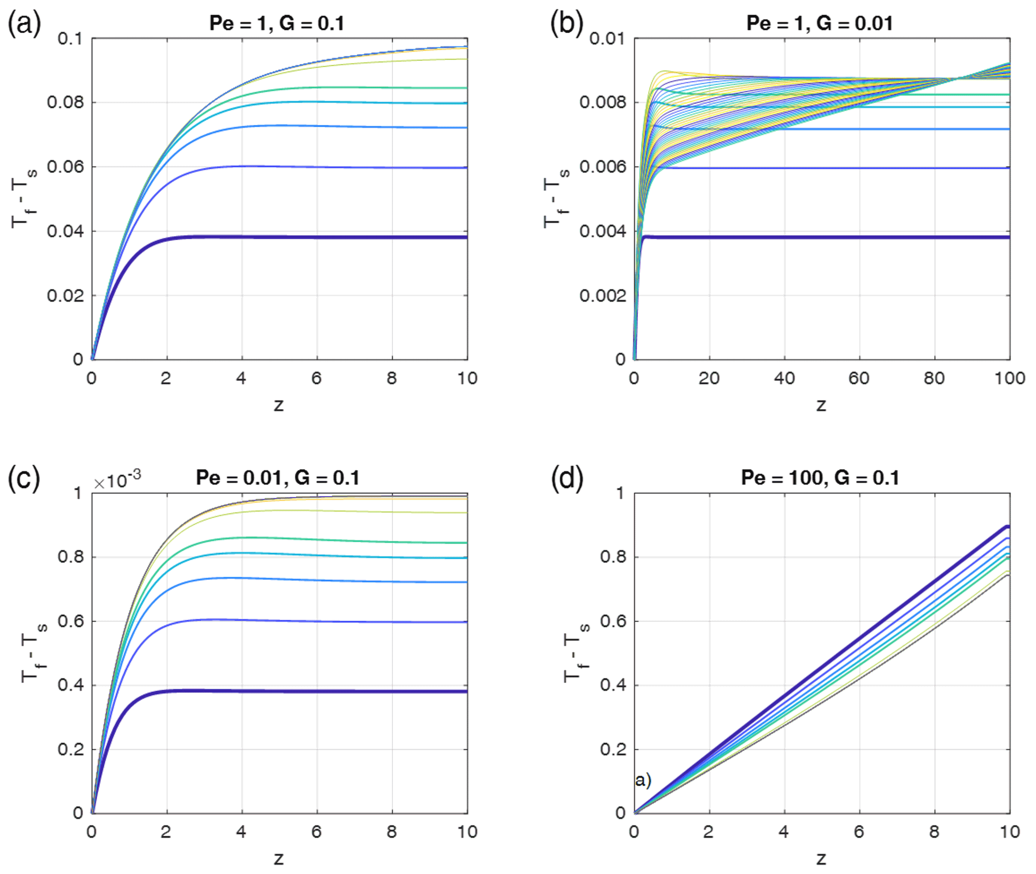
Figure 9 Time- and depth-dependent profiles of the fluid–solid temperature differences as in Fig. 5, but for fluid-to-solid property ratios typical for water flowing through sedimentary rocks, i.e., ${\mathit{\rho }}_{\mathrm{s}}^{\prime }{c}_{p,\mathrm{s}}^{\prime }=\mathrm{0.78}$, ${\mathit{\kappa }}_{\mathrm{s}}^{\prime }=\mathrm{16}$, and ${\mathit{\lambda }}_{\mathrm{eff}}^{\prime }=\mathrm{1}$. Pe and G have been chosen as indicated in the panel titles (as in Fig. 5), and ϕ=0.1 was assumed. In each panel the curves show (T_f−T_s) profiles for progressive times, and the colors are cyclically varied with time from blue to yellow, starting with blue (bold curve). The first five curves were taken with time increments of 0.4875 and the later curves with 4.875. The total time was 100 in all models with G=0.1 and 200 in the models with G=0.01. Steady state is reached in the models with G=0.1. The model with G=0.01 would need t = 10 000 to reach steady state.

5.2 Timescales

It is interesting to evaluate the timescales for reaching the maximum non-equilibrium temperature differences and the steady state. For every numerical model, we recorded the time needed to reach 90 % of the maximum temperature differences between fluid and solid, t_90 %, and the time needed to reach steady state, t_steady. The latter has been determined as the time at which the maximum difference between (T_f(z)−T_s(z)) curves at two subsequent time steps becomes less than ${\mathrm{10}}^{-\mathrm{8}}\mathrm{\Delta }{T}_{max}$. These times can be compared with different timescales that may characterize the evolution of temperatures in the models. These timescales can be based on advection over a characteristic distance d_char, giving $t_{\mathrm{advd}}=d_{\mathrm{char}}/v_{\mathrm{f}\mathrm{0}}$, or on diffusion over the characteristic distance, giving $t_{\mathrm{diffd}}=d_{\mathrm{char}}^{\mathrm{2}}/{\mathit{\kappa }}_{\mathrm{0}}$. We tested these timescales with the two natural length scales of the models. The first is the scaling length L (equal to 1 non-dimensional), representing essentially the geometric mean of the channel width of the pores, d_f, and the interfacial boundary layer thickness δ. The second is the model height H. Grouping the models depending on the regime they belong to (see Sect. 4.3.4 and Fig. 4), we plotted the recorded times t_90 % and t_steady versus the characteristic timescales mentioned above. Good agreement with the characteristic timescales is indicated by observed times fitting to the dashed x=y lines (Fig. 10).

Figure 10 For evaluating timescales the numerically determined times of models with various parameters Pe and G representing the three different regimes 1, 2, and 3 (different symbols) are plotted against characteristic scaling times. (a) Times for reaching 90 % of the maximum temperature difference ΔT_max are plotted against either the advective timescale t_advH based on model height H for regime 1 models or against the scaling time t₀ for regime 2 models, or against the diffusive timescale t_diffH based on the model height H. (b) Times for reaching steady states are plotted against the characteristic diffusive timescales, t_diffH, based on model height H for all three regimes. Models close to the dashed line (y=x) are in best agreement with the characteristic times. In (a) regime 2 times are taken dimensionally by multiplying the observed times and the non-dimensional scaling time $t_{\mathrm{0}}^{\prime }=\mathrm{1}$ by some arbitrary dimensional times t₀.

In regime 1 (high Pe), t_90 % is proportional to t_advH (Fig. 10a, blue circles). In this regime the high value of Pe makes the fluid temperature increase fast. It reaches its maximum value during the time under which significant fluid–solid heat transfer builds up and the solid temperature is still low. This corresponds to the time for traveling the full distance H. During stages 2 and 3 the solid temperature increases and the temperature difference decreases before steady state is reached. The time for reaching steady state (Fig. 10b, circles) varies roughly linearly with t_steady∝t_diffH. For most cases it is controlled by diffusion through the solid over distances of the order of H. The case with large H (circle in Fig. 10b below dashed line) apparently reaches the steady state earlier, but still later than on a corresponding advective timescale based on H (not shown). Inspecting this model shows that during stages 2 and 3 the high Pe number facilitates approaching thermal equilibrium rapidly within large parts of the model and reducing the effective length scale (and characteristic timescale) over which non-equilibrium is still present.

In regime 2 (low Pe and G<0.1, i.e., H>10) the time for reaching ΔT_max is controlled by interfacial heat transfer (Fig. 10a, red asterisks) on the length scale L, resulting in t_90 % proportional to t₀. The time for reaching steady state is controlled by the diffusion timescale across the height of the system (Fig. 10b).

In regime 3 (low Pe and high G (small H)), time for reaching ΔT_max is similar to or shorter than the diffusion time based on the model height H (Fig. 10a, black crosses). The flattening of the curve indicates that non-equilibrium is reached faster for some models because Pe reaches the order of 1 and the advective timescale starts to take over. The time for reaching steady state (Fig. 10b, crosses) varies linearly with t_steady∝t_diffH. Clearly, it is also controlled by diffusion.

5.3 Applications to magmatic systems

We now test the possible occurrence of thermal non-equilibrium in natural magmatic systems based on the suggested controlling non-dimensional parameters, namely the Péclet number Pe, the initial thermal gradient G ($=\mathrm{1}/H$), and the melt fraction ϕ. Typical stages of melt flow for mid-ocean ridges include three stages:

• a.

  partially molten regions with interstitial melts sitting at grain corners, grain edges, or grain faces with low (0.0001 %–6 %) melt fractions (see, e.g., the discussion in Schmeling, 2006);

• b.

  merging melt channel or vein systems with high-porosity (> 10 %–20 %) channels identified as dunite channels after complete melt extraction (Kelemen et al., 1997);

• c.

  propagating dikes or other volcanic conduits.

Let us assume typical overall melt fractions of 1 % to 20 % for stages (b) and (c). Schmeling et al. (2018) discussed possible Péclet numbers for such systems based on a Darcy-flow-related Péclet number:

$$\begin{array}{}\text{(33)}& {\mathit{Pe}}_{\mathrm{D}}={\displaystyle \frac{v_{\mathrm{D}}{d}_{\mathrm{s}}}{{\mathit{\kappa }}_{\mathrm{0}}}}.\end{array}$$

As we preferably use the melt pore dimension d_f in our scalings (Eqs. 9a and 10a), we need to relate it to the solid phase dimension d_s by using

$$\begin{array}{}\text{(34)}& d_{\mathrm{s}}=d_{\mathrm{f}}{\displaystyle \frac{g}{\mathit{\varphi }}},g=\left\{\begin{array}{ll}\left(\mathrm{1}-\mathit{\varphi }\right)& \text{melt channels}\\ \sqrt{\mathit{\varphi }}\left(\mathrm{1}-\sqrt{\mathit{\varphi }}\right)& \text{melt tubes}.\end{array}\right.\end{array}$$

Using Eqs. (34), (9a), and (16), we arrive at the Péclet number used here.

$$\begin{array}{}\text{(35)}& \mathit{Pe}={\mathit{Pe}}_{\mathrm{D}}{\displaystyle \frac{\mathrm{1}}{g\sqrt{c}}}\sqrt{{\displaystyle \frac{\left(\mathrm{1}-\mathit{\varphi }\right)\mathit{\delta }}{d_{\mathrm{f}}}}}\end{array}$$

Schmeling et al. (2018) reviewed and estimated typical pore or channel spacings d_s of 10⁻³–10⁻² m for stage (a), 0.1 m for early stage (b) increasing to 1–100 m for late stage (b), and 100–300 m for stage (c) (dikes). Arguing for typical geometries, spreading rates, and melt extraction rates, Schmeling et al. (2018) estimated the Darcy velocity to range between 10⁻¹⁰ and 10⁻⁹ m s⁻¹. With these parameters Pe_D numbers for the three stages can be estimated for the three stages as

• a.

  10⁻⁷ to 10⁻⁵,

• b.

  10⁻⁵ to 10⁻⁴ at depths where channel distances are of the order of 0.1 m and 10⁻⁴ to 0.1 at shallower depths where the channel distances have increased to the order of 1 to 100 m,

• c.

  >10⁵ for the dike stage.

To estimate Péclet numbers as defined here (Eq. 35), typical interfacial thermal boundary layer thicknesses δ are needed. As the thermal interfacial heat exchange intrinsically is time-dependent, a good estimate is $\mathit{\delta }=c_{\mathrm{th}}\sqrt{{\mathit{\kappa }}_{\mathrm{0}}t}$ (in dimensional form), where c_th is a constant for a thermal boundary layer, equal to 2.32 for a cooling half space (Turcotte and Schubert, 2014). Assuming that the characteristic time can be expressed by the (dimensional) fluid velocity v₀ and system height H, i.e., by $t=H/v_{\mathrm{0}}=H\mathit{\varphi }/v_{\mathrm{D}}$, we may express v_D in terms of the Péclet number Pe_D. With the resulting t and δ we arrive at the following Péclet number (H and d_f are dimensional or non-dimensional):

$$\begin{array}{}\text{(36)}& \mathit{Pe}={\mathit{Pe}}_{\mathrm{D}}^{\mathrm{3}/\mathrm{4}}\sqrt{{\displaystyle \frac{c_{\mathrm{th}}}{c}}}{g}^{-\mathrm{3}/\mathrm{4}}{\left({\displaystyle \frac{H}{d_{\mathrm{f}}}}\right)}^{\mathrm{1}/\mathrm{4}}\sqrt{\mathrm{1}-\mathit{\varphi }}.\end{array}$$

For mid-ocean ridge settings we assume H to represent the transition region between the lithosphere and asthenosphere with a thickness of the order of 1 to 10 km, and we use Eq. (34) to insert typical d_f values. They increase from 10⁻⁴ m for interstitial melts (stage a) to 10⁻³ to 10⁻¹ m for the channeling stage (b) (see Schmeling et al., 2018) to >10 m for the dike stage (c). The resulting Péclet number (Eq. 36) is of the order of 10⁻³ to 0.5 for stage a, 10⁻² during the early stage (b) and 10⁻² to 1 during the later stage (b) appropriate for dunite systems, and 10⁴ to 10⁷ for the dike stage (c). To estimate typical non-dimensional thermal gradients G^′ (or layer thickness H^′), the above estimate for δ and d_f can be inserted into the scaling length L (Eq. 9a) to arrive at a non-dimensional $G^{\prime }=\mathrm{1}/H^{\prime }$.

$$\begin{array}{}\text{(37)}& G^{\prime }={\left({\displaystyle \frac{H}{d_{\mathrm{s}}}}\right)}^{-\mathrm{3}/\mathrm{4}}{g}^{-\mathrm{1}/\mathrm{2}}{\mathit{\varphi }}^{\mathrm{3}/\mathrm{4}}\sqrt{{\displaystyle \frac{c_{\mathrm{th}}}{c}}}{\mathit{Pe}}_{\mathrm{D}}^{-\mathrm{1}/\mathrm{4}}\sqrt{\mathrm{1}-\mathit{\varphi }}\end{array}$$

With the derived estimates for the three stages, G^′ is of the order of 10⁻⁶ to 10^−2.7 for stage (a), 10⁻⁴–10^−2.5 increasing to 10⁻⁴–0.6 for stage (b), and 10⁻⁵–10⁻² for the dike stage (c). These resulting stages for Pe and G^′ are indicated in the regime diagram (Fig. 4). All three stages extend far into the domain, with G values smaller than 0.001. Thermal non-equilibrium of the three stages can be summarized as follows.

• a.

  Interstitial melts are at full thermal equilibrium.

• b.

  Channeling and veining may result in moderate thermal non-equilibrium at sufficiently high thermal gradients.

• c.

  After transition to diking full thermal non-equilibrium is predicted.

A similar exercise can be done for continental magmatic systems. We skip such an explicit evaluation here but note that silicic melt viscosities are typically higher than those of basaltic melts at mid-ocean ridges. Thus, Péclet numbers are expected to be smaller, but non-dimensional thermal gradients (Eq. 37) might be larger, resulting in a downward and rightward shift of the natural stages indicated in Fig. 4.

To make our scaling laws and timescales for reaching maximum thermal non-equilibrium more accessible, it is worth writing them in dimensional form. First, to estimate the Péclet number of a natural system, combining Eqs. (9) and (16) gives

$$\begin{array}{}\text{(38)}& \mathit{Pe}={\displaystyle \frac{v_{\mathrm{f}\mathrm{0}}}{{\mathit{\kappa }}_{\mathrm{0}}}}\sqrt{{\displaystyle \frac{{\mathit{\varphi }}_{\mathrm{0}}\left(\mathrm{1}-{\mathit{\varphi }}_{\mathrm{0}}\right)\mathit{\delta }}{S}}},\end{array}$$

indicating that for very small or very large melt fractions Pe becomes very small. One may use Eqs. (11) or (12) to write Pe also in terms of pore or solid (grain or channel spacing) dimensions d_f or d_s, respectively. The scaling laws and characteristic timescales for the three regimes we found (Fig. 4) are in dimensional form.

• Regime 1. For large Pe values the maximum non-equilibrium temperature difference is simply equal to the imposed temperature difference, $\mathrm{\Delta }{T}_{max}=\mathrm{\Delta }{T}_{\mathrm{0}}$, and the characteristic time to reach maximum non-equilibrium is simply $t_{\mathrm{char}}=H/v_{\mathrm{f}\mathrm{0}}$, i.e., the total time of a fluid particle for passing through the system.

• Regimes 2 and 3. For small Péclet numbers ($\mathit{Pe}<\frac{H\sqrt{S}}{\sqrt{{\mathit{\varphi }}_{\mathrm{0}}\left(\mathrm{1}-{\mathit{\varphi }}_{\mathrm{0}}\right)\mathit{\delta }}}$) the maximum temperature difference scales like

  $$\begin{array}{}\text{(39)}& \begin{array}{rl}\mathrm{\Delta }{T}_{max}& ={\displaystyle \frac{G{v}_{\mathrm{f}\mathrm{0}}{\mathit{\varphi }}_{\mathrm{0}}\left(\mathrm{1}-{\mathit{\varphi }}_{\mathrm{0}}\right)\mathit{\delta }}{{\mathit{\kappa }}_{\mathrm{0}}S}}\\ & ={\displaystyle \frac{v_{\mathrm{f}\mathrm{0}}{\mathit{\varphi }}_{\mathrm{0}}\left(\mathrm{1}-{\mathit{\varphi }}_{\mathrm{0}}\right)\mathit{\delta }}{H{\mathit{\kappa }}_{\mathrm{0}}S}}\mathrm{\Delta }{T}_{\mathrm{0}},\end{array}\end{array}$$

  and the characteristic time for reaching this non-equilibrium scales with t₀, i.e.,

  $$\begin{array}{}\text{(40)}& t_{\mathrm{char}}={\displaystyle \frac{{\mathit{\varphi }}_{\mathrm{0}}\left(\mathrm{1}-{\mathit{\varphi }}_{\mathrm{0}}\right)\mathit{\delta }}{{\mathit{\kappa }}_{\mathrm{0}}S}}.\end{array}$$

  These relations can easily be used to assess the potential of thermal non-equilibrium in systems of fluid flow through solids with given geometrical properties and fluid fractions.

In the above discussion we used the terms moderate thermal non-equilibrium, which we may identify with $\mathrm{\Delta }{T}_{max}^{\prime }$ of a few percent to, say, 30 %, while full thermal non-equilibrium includes higher values up to 100 %. To translate this into dimensional ΔT_max values, what are typical ΔT₀ values for mid-ocean ridges? In our example we defined Has the thickness of the transition region between lithosphere and asthenosphere. Such a transition zone may be defined by the depth region bounded by the asthenospheric temperature T_asth and, say, 0.8T_asth, i.e., $\mathrm{\Delta }{T}_{\mathrm{0}}=\mathrm{0.2}{T}_{\mathrm{asth}}\cong \mathrm{200}$ K. Thus moderate non-equilibrium may be represented by excess temperatures of the melt with respect to the solid between, say, 6 and 60 K, while full thermal non-equilibrium suggests the full ΔT₀ range of 60 to 200 K or even higher in the case of dikes extending up into the lithosphere with temperatures below 0.8 T_asth. These typical temperature estimates may have some implications for whether the solid rock will melt or the melt will freeze. However, this discussion is beyond the scope of this paper.

6 Conclusions

In conclusion, we showed that in magmatic systems characterized by two-phase flows of melts with respect to solid, thermal non-equilibrium between melt and solid may arise and becomes important under certain conditions. The main conclusions are summarized as follows.

From non-dimensionalization of the governing equations, three non-dimensional numbers can be identified controlling thermal non-equilibrium: the Péclet number Pe, the melt porosity ϕ, and the initial non-dimensional temperature gradient G in the system. The maximum possible non-equilibrium solid–fluid temperature difference ΔT_max is controlled only by two non-dimensional numbers: Pe and G. Both numerical and analytical solutions show that in a Pe–G parameter space three regimes can be identified.

• In regime 1 (high $\mathit{Pe}(>\mathrm{1}/G)$) strong thermal non-equilibrium develops independently of Pe, and a non-dimensional scaling law $T_{\mathrm{f}}-T_{\mathrm{s}}=Gz$ has been derived.

• In regime 2 (low $\mathit{Pe}(<\mathrm{1}/G)$ and low G(<0.3)) non-equilibrium decreases proportionally to decreasing Pe and G, and the non-dimensional scaling law reads $T_{\mathrm{f}}-T_{\mathrm{s}}=\mathit{Pe}G\left(\mathrm{1}-e^{-z}\right)$.

• In regime 3 (low Pe(<1) and G of the order of 1) non-equilibrium scales with Pe and G and is depth-dependent. The scaling law is $T_{\mathrm{f}}-T_{\mathrm{s}}=\mathit{Pe}G\left(\mathrm{1}-M\left(z\right)\right)$, where M(z) depends on G.

Further conclusions include the following.

• The timescales for reaching thermal non-equilibrium scale with the advective timescale in the high-Pe regime and with the interfacial diffusion time in the other two low-Pe-number regimes.

• Applying the results to natural magmatic systems such as mid-ocean ridges can be done by estimating appropriate orders of Pe and G. Plotting such typical ranges in the Pe–G regime diagram reveals that (a) interstitial melt flow is in thermal equilibrium, (b) melt channeling as revealed by dunite channels, for example, may reach moderate thermal non-equilibrium, and (c) the dike regime is at full thermal non-equilibrium.

• In the studied setup G was constant, leading to conservative estimates of thermal non-equilibrium. Any other depth-dependent initial temperature distributions generate higher non-equilibrium than reported here.

• The derived scaling laws for thermal non-equilibrium are valid for equal solid and fluid properties. Assuming different properties such as for a water–sandstone system results in similar maximum non-equilibrium temperature differences, but in significantly different time evolutions.

While for simplicity the presented approach has been done essentially for constant model parameters, it can easily be extended to vertically varying parameters. Thus, tools are provided for evaluating the transition from thermal equilibrium to non-equilibrium for anastomosing systems (Hart, 1993).