An efficient partial-differential-equation-based method to compute pressure boundary conditions in regional geodynamic models

Modelling the pressure in the Earth's interior is a common problem in Earth sciences. In this study we propose a method based on the conservation of the momentum of a fluid by using a hydrostatic scenario or a uniformly moving fluid to approximate the pressure. This results in a partial differential equation (PDE) that can be solved using classical numerical methods. In hydrostatic cases, the computed pressure is the lithostatic pressure. In non-hydrostatic cases, we show that this PDE-based approach better approximates the total pressure than the classical 1D depth-integrated approach. To illustrate the performance of this PDE-based formulation we present several hydrostatic and non-hydrostatic 2D models in which we compute the lithostatic pressure or an approximation of the total pressure, respectively. Moreover, we also present a 3D rift model that uses that approximated pressure as a time-dependent boundary condition to simulate far-field normal stresses. This model shows a high degree of non-cylindrical deformation, resulting from the stress boundary condition, that is accommodated by strike-slip shear zones. We compare the result of this numerical model with a traditional rift model employing free-slip boundary conditions to demonstrate the first-order implications of considering “open” boundary conditions in 3D thermo-mechanical rift models.

1 Introduction

In Earth sciences and geodynamic modelling, computing the pressure can be essential. Specifically, numerous regional thermo-mechanical studies use the lithostatic pressure or a reference pressure based on some density structure as a normal stress boundary condition (e.g. Baes et al., 2018; Brune, 2014; Brune et al., 2012, 2014, 2017; Chertova et al., 2012, 2014; Glerum et al., 2018; Ismail-Zadeh et al., 2013; Popov and Sobolev, 2008; Quinteros et al., 2010; Yamato et al., 2008). By imposing only the normal stress, material is permitted to flow in and out of the domain in response to the other boundary conditions and or deformation in the domain interior. This is inherently closer to the reality of the dynamics within a regional segment of the Earth,compared to a regional domain that is closed and in which neither inflow nor outflow is permitted. Hence, the ultimate intent of imposing the normal stress is to provide dynamical behaviour that is similar to that which would occur if the models were performed in a much larger domain. Moreover, the reference pressure can also be used as an initial guess for the pressure when solving linear or non-linear system flow problems with iterative methods.

The common approach to compute a reference pressure P is to define a set of depth columns and integrate the rock density ρ(x) over each column to obtain the pressure at depth. Thus, to compute the pressure P at some point of x^′, we evaluate the 1D integral as follows:

$$\begin{array}{}\text{(1)}& P\left({\mathit{x}}^{\prime }\right)=P_{\mathrm{s}}+\underset{{\mathit{x}}_{\mathrm{s}}^{\prime }}{\overset{{\mathit{x}}^{\prime }}{\int }}\mathit{\rho }\left(\mathit{x}\right)\left|\right|\mathit{g}\left(\mathit{x}\right)\left|\right|\mathrm{d}x,\end{array}$$

where ${\mathit{x}}_{\mathrm{s}}^{\prime }$ is the projection of x^′ onto the surface of the Earth in the direction opposite to the gravity vector g and P_s is the reference pressure at the surface ${\mathit{x}}_{\mathrm{s}}^{\prime }$. For the case of a constant density and gravity, this expression reduces to $P\left({\mathit{x}}^{\prime }\right)=P_{\mathrm{s}}+\mathit{\rho }gD$, where D is the distance (depth) given by $D=\Vert {\mathit{x}}_{\mathrm{s}}^{\prime }-{\mathit{x}}^{\prime }\left|\right|$ and $g=\left|\right|\mathit{g}\left|\right|$. When the density is a function of space and gravity is constant, the 1D integral is decomposed into different segments D_i and a suitable quadrature rule is applied over each segment. For example using a one-point Gauss quadrature rule we have

$$\begin{array}{}\text{(2)}& P\left({\mathit{x}}^{\prime }\right)=P_{\mathrm{s}}+\sum _i\underset{D_i}{\int }\mathit{\rho }\left(\mathit{x}\right)g\mathrm{d}x\approx P_{\mathrm{s}}+\sum _i{\mathit{\rho }}_{i}g{D}_i,\end{array}$$

where ρ_i is the density at the centroid of the segment D_i. For the case of a uniform mesh with cell edges aligned with the gravity vector, all the cell edges and vertices are located along straight lines that are parallel to the direction of gravity. Hence, Eq. (2) can be simply evaluated by traversing along a column associated with a set of cells (or vertices). In this special case, the sub-division of the integral is naturally defined by mesh cells. If the column sweep is performed from the surface to depth, then only a single pass over each cell in a column is required to compute the pressure at any depth within that column by accumulating values from cells at shallower depths. Therefore, if we traverse from segments i = 0, 1, 2, …, N, where the segments are ordered such that D_i+1 is located at greater depth than D_i, then we have the following sequence $P_{\mathrm{0}}=P_{\mathrm{s}}+{\mathit{\rho }}_{\mathrm{0}}g{D}_{\mathrm{0}}$, $P_{\mathrm{1}}=P_{\mathrm{s}}+{\mathit{\rho }}_{\mathrm{0}}g{D}_{\mathrm{0}}+{\mathit{\rho }}_{\mathrm{1}}g{D}_{\mathrm{1}}=P_{\mathrm{0}}+{\mathit{\rho }}_{\mathrm{1}}g{D}_{\mathrm{1}}$, …, $P_N=P_{\mathrm{s}}+{\sum }_i^N{\mathit{\rho }}_{i}g{D}_i=P_{N-\mathrm{1}}+{\mathit{\rho }}_{N}g{D}_N$.

Although evaluating Eq. (2) may appear simple, its implementation may be inefficient or too algorithmically complex for general use. Below we outline some common use cases that render the column-wise integration difficult (or expensive):

1. a mesh with cell edges (2D) or faces (3D) that are not aligned with the gravity vector (Fig. 1a),

2. an unstructured mesh (Fig. 1b),

3. a density structure (or gravity vector) that is spatially varying,

4. a parallel decomposition of the mesh (Fig. 1c),

5. time dependence in the density or mesh coordinates that requires continual re-evaluation of the reference pressure.

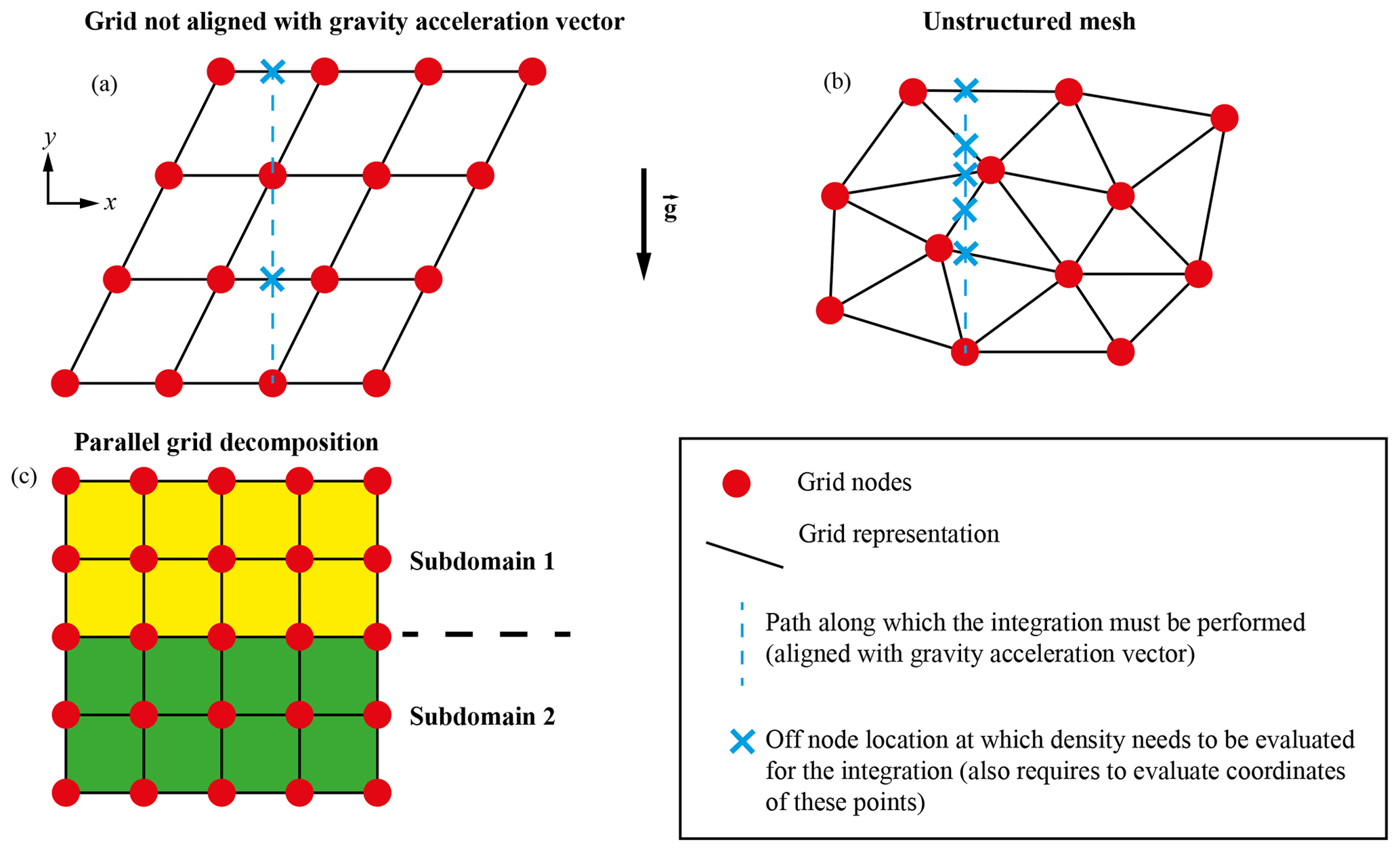
Figure 1 Schematic representation of meshes for which computing an integral in the vertical direction can be challenging: (a) mesh with a grid not aligned with the gravity vector, (b) unstructured mesh, and (c) parallel distribution of a mesh. The dashed blue lines represent the direction along which the integral must be performed. The blue crosses represent the points that have to be evaluated during the integration.

To compute P(x^′) we first have to define the location ${\mathit{x}}_{\mathrm{s}}^{\prime }$. In general this is non-trivial for use cases (1) and (2). If both the density and gravity are constant, then the only complexity associated with meshes identified in points (1) and (2) relate to computing ${\mathit{x}}_{\mathrm{s}}^{\prime }$. Due to the fact that the path of the integral (i.e. the “column”) does not coincide in general with a set of mesh cells or vertices, the line integral must be performed for each point x^′ in the mesh, meaning that the single pass approach used in the gravity-aligned mesh is not possible. If the density (or gravity) vary in space throughout the domain, the integral must be approximated via a suitable sub-division in space and/or a quadrature rule. Assuming that the density is a piecewise constant over each cell, the simplest approximation would be to determine the intersection between the line segment $[{\mathit{x}}^{\prime },{\mathit{x}}_{\mathrm{s}}^{\prime }]$ and each cell and apply a one-point quadrature rule over the intersecting segment times. In Fig. 1a and b we depict the complexity of this procedure for a non-coordinate-aligned and unstructured mesh. When performing simulations in parallel where the mesh is distributed across multiple Message Passing Interface (MPI) ranks, even for the case of a uniform mesh aligned with the gravity vector, the column-wise integration approach is somewhat complicated. Individual MPI ranks may compute their local contribution to the sum of accumulated pressures; however, the final pressure requires a partial sum to be performed over mesh sub-domains that intersect the 1D line integral. The global reduction (with the chosen MPI ranks overlapping with each 1D line integral) is complicated to define for mesh types identified in points (1) and (2). Lastly, if the reference pressure associated with some density structure is to be used as a boundary condition in a mechanical model, time dependence of that density structure (or mesh) will require one to re-compute the reference pressure at each time step. Hence, the efficiency of the implementation used to compute the pressure is important.

Moreover, when the density structure evolves with time as deformation occurs, the pressure gradients may no longer be aligned with the gravitational acceleration vector. In these non-hydrostatic cases, this pressure is not lithostatic. However, to be able to provide an approximation for the total pressure or to use stress boundary conditions, it is still important to approximate the total pressure in the best possible way.

For these reasons, we propose an efficient mesh and numerical method (finite elements, finite differences, finite volumes, etc.) to compute a reference pressure associated with the density structure of a domain in hydrostatic cases or an approximation of the total pressure for non-hydrostatic cases for all scenarios given above by solving a partial differential equation (PDE) derived from the conservation of the non-inertial momentum equation for an incompressible fluid. We also present thermo-mechanical numerical models and static numerical models applied to Earth sciences and geodynamics to show the usefulness of this approach.

2 PDE-based pressure formulation

For an incompressible fluid in a domain Ω, the non-inertial form of the conservation of momentum is given by the Stokes equation

$$\begin{array}{}\text{(3)}& \mathrm{\nabla }\cdot \mathit{\tau }-\mathrm{\nabla }P+\mathit{\rho }\mathit{g}=\mathbf{0},\end{array}$$

where v is the velocity of the fluid, P is the total pressure, $\mathit{\tau }=\mathrm{2}\mathit{\eta }\dot{\mathit{\epsilon }}\left(\mathit{v}\right)$ is the deviatoric stress tensor with η the viscosity, $\dot{\mathit{\epsilon }}\left(\mathit{v}\right)$ is the strain rate tensor, $\mathit{\rho }:=\mathit{\rho }(\mathit{x},t)$ is the density, $\mathit{g}:=\mathit{g}(\mathit{x},t)$ is the gravity vector, and x and t denote the space and time, respectively. The incompressibility constraint is given as follows:

$$\begin{array}{}\text{(4)}& \mathrm{\nabla }\cdot \mathit{v}=\mathrm{0}.\end{array}$$

In the context of our problems we will decompose the boundary of the domain into two non-overlapping segments: ∂Ω_surf that we will regard as the free surface and prescribe that tangential and normal stresses are zero, i.e. $\mathit{\tau }-P\mathbb{I}=\mathbf{0}$, and ∂Ω_i, which denotes the interior parts of the boundary along which we may impose any valid combination of velocity or stress in the normal and tangential directions. Furthermore, $\partial \mathrm{\Omega }=\partial {\mathrm{\Omega }}_{\text{i}}\cup \partial {\mathrm{\Omega }}_{\mathrm{surf}}$ and $\partial {\mathrm{\Omega }}_{\text{i}}\cap \partial {\mathrm{\Omega }}_{\mathrm{surf}}=\mathrm{\varnothing }$. The outward-pointing unit normal vector to ∂Ω will be denoted via $\widehat{\mathit{n}}$.

To define the pressure associated with the density structure we make the “ansatz” that v=0; hence, Eq. (4) is trivially satisfied, and Eq. (3) reduces to the usual hydrostatic equilibrium problem

$$\begin{array}{}\text{(5)}& \mathbf{0}=-\mathrm{\nabla }P+\mathit{\rho }\mathit{g}.\end{array}$$

For spatial dimensions $n_{\mathrm{d}}=\mathrm{2},\mathrm{3}$, Eq. (5) is over-determined as there are more equations (n_d) than unknowns:

$$\begin{array}{}\text{(6)}& \left[\begin{array}{c}\frac{\partial }{\partial x}\\ \frac{\partial }{\partial y}\\ \frac{\partial }{\partial z}\end{array}\right]P=\mathit{\rho }\left(\mathit{x}\right)\left[\begin{array}{c}{g}_x\\ g_y\\ g_z\end{array}\right].\end{array}$$

As such, there is no unique solution to Eq. (5). To obtain a unique solution to Eq. (5), we require a single equation for P. This can be achieved by taking the divergence of Eq. (5):

$$\begin{array}{}\text{(7)}& \mathrm{\nabla }\cdot \mathrm{\nabla }P=\mathrm{\nabla }\cdot \left(\mathit{\rho }\mathit{g}\right).\end{array}$$

Eq. (7) will be referred to as the pressure Poisson equation (PPE).

Equation (7) can be obtained in an alternative manner with less restrictive assumptions. First, we assume that we have a solution ((v),p) for Eqs. (3), (4). Then we take the divergence of the momentum equation (as before) and integrate over Ω

$$\begin{array}{}\text{(8)}& \underset{\mathrm{\Omega }}{\int }\mathrm{\nabla }\cdot (\mathrm{\nabla }\cdot \mathit{\tau })\mathrm{d}V-\underset{\mathrm{\Omega }}{\int }\mathrm{\nabla }\cdot \mathrm{\nabla }P\mathrm{d}V+\underset{\mathrm{\Omega }}{\int }\mathrm{\nabla }\cdot \left(\mathit{\rho }\mathit{g}\right)\mathrm{d}V=\mathrm{0}.\end{array}$$

Then, applying the divergence theorem to the first term we obtain

$$\begin{array}{}\text{(9)}& \underset{\partial \mathrm{\Omega }}{\int }(\mathrm{\nabla }\cdot \mathit{\tau })\cdot \widehat{\mathit{n}}\mathrm{d}S-\underset{\mathrm{\Omega }}{\int }\mathrm{\nabla }\cdot \mathrm{\nabla }P\mathrm{d}V+\underset{\mathrm{\Omega }}{\int }\mathrm{\nabla }\cdot \left(\mathit{\rho }\mathit{g}\right)\mathrm{d}V=\mathrm{0}.\end{array}$$

If we assume the boundary term on the left-hand side is small, we have

$$\begin{array}{}\text{(10)}& \underset{\mathrm{\Omega }}{\int }\mathrm{\nabla }\cdot \mathrm{\nabla }P\mathrm{d}V\approx \underset{\mathrm{\Omega }}{\int }\mathrm{\nabla }\cdot \left(\mathit{\rho }\mathit{g}\right)\mathrm{d}V\end{array}$$

which must be true for any arbitrary domain, thus resulting in Eq. (7).

Assuming that $\widehat{\mathit{n}}$ is constant or slowly varying and that τ is symmetric yields

$$\begin{array}{}\text{(11)}& (\mathrm{\nabla }\cdot \mathit{\tau })\cdot \widehat{\mathit{n}}=n_i{\displaystyle \frac{\partial }{\partial x_j}}{\mathit{\tau }}_{ij}\approx {\displaystyle \frac{\partial }{\partial x_j}}\left({\mathit{\tau }}_{ji}{n}_i\right)=\mathrm{\nabla }\cdot \left(\mathit{\tau }\widehat{\mathit{n}}\right).\end{array}$$

Hence, dropping the first term in Eq. (9) is equivalent to saying that $\mathit{\tau }\widehat{\mathit{n}}\approx \mathbf{0}$ for all $\mathit{x}\in \partial \mathrm{\Omega }$. Alternatively, the term is zero if $\mathrm{\nabla }\cdot \mathit{\tau }=\mathbf{0}$ for all $\mathit{x}\in \partial \mathrm{\Omega }$. This condition is satisfied if the fluid experiences either rigid body translations or rigid body rotation along ∂Ω.

2.1 Boundary conditions

A unique solution to Eq. (7) requires boundary conditions to be specified on P. Our choice of boundary conditions for Eq. (7) is motivated by Earth-like bodies. The boundary conditions will be specified in the usual manner, i.e. in terms of a Dirichlet constraint in which we impose P and Neumann constraints in which we impose the behaviour of $\mathrm{\nabla }P\cdot \widehat{\mathit{n}}$.

Along the surface of the domain, which represents the free surface of the Earth, we impose

$$\begin{array}{}\text{(12)}& P=\mathrm{0}\text{for all}\mathit{x}\in \partial {\mathrm{\Omega }}_{\mathrm{surf}}.\end{array}$$

Equation (12) is a Dirichlet constraint and specifies that the reference (or datum) pressure should be zero on the surface of our geological body. This is consistent with the observation that the mean pressure on all points on the surface (above sea level) are approximately equal. This Dirichlet boundary condition is a natural extension of the free surface boundary condition used for the flow problem in Eqs. (3), (4), namely $\widehat{\mathit{n}}\cdot (\mathit{\tau }-P\mathbb{I})\widehat{\mathit{n}}=\widehat{\mathit{n}}\cdot (\mathit{\tau }-P\mathbb{I})\widehat{\mathit{t}}=\mathrm{0}$, which reduces to $\widehat{\mathit{n}}\cdot \mathit{\tau }\widehat{\mathit{n}}-P=\mathrm{0}$ and $\widehat{\mathit{n}}\cdot \mathit{\tau }\widehat{\mathit{t}}=\mathrm{0}$ with $\widehat{\mathit{t}}$ a tangent unit vector to the boundary such that $\widehat{\mathit{n}}\cdot \widehat{\mathit{t}}=\mathrm{0}$. Equation (12) is consistent with a fluid at rest since τ=0. In the non-hydrostatic case, we require $\mathit{\tau }\widehat{\mathit{n}}\approx \mathrm{0}$ to arrive at Eq. (12). We also note that $\widehat{\mathit{n}}\cdot \mathit{\tau }\widehat{\mathit{n}}$ is proportional to the mean curvature κ of the boundary ∂Ω (Barth and Carey, 2007). Hence, if there is zero topography, κ=0 and P=0 on ∂Ω_surf, and if the change in topography is small, then κ≈0 and P≈0.

Two different boundary conditions are introduced to constrain $\mathrm{\nabla }P\cdot \widehat{\mathit{n}}$. These are defined as a direct extension of the 1D hydrostatic assumptions to 2D and 3D domains. We first introduce some additional quantities that will aid the definition of the Neumann boundary condition. First, we split ∂Ω_i into two parts, such that $\partial {\mathrm{\Omega }}_i=\partial {\mathrm{\Omega }}_{⟂}\cup \partial {\mathrm{\Omega }}_{\parallel }$. Next, we define the gravity unit vector $\widehat{\mathit{g}}$ such that

$$\begin{array}{}\text{(13)}& \mathit{g}=g\widehat{\mathit{g}},\end{array}$$

and the unit vector ${\widehat{\mathit{g}}}_{⟂}$, which is perpendicular to $\widehat{\mathit{g}}$, i.e.

$$\begin{array}{}\text{(14)}& \widehat{\mathit{g}}\cdot {\widehat{\mathit{g}}}_{⟂}=\mathrm{0}.\end{array}$$

The first constraint states that P should increase only in the direction of gravity. Hence, from Eq. (5) we have

$$\begin{array}{}\text{(15)}& \mathrm{\nabla }P\cdot \widehat{\mathit{g}}=\mathit{\rho }g\Vert \widehat{\mathit{g}}{\Vert }^{\mathrm{2}}=\mathit{\rho }g,\text{for all}\mathit{x}\in \partial {\mathrm{\Omega }}_{\parallel }.\end{array}$$

The second constraint states that P should not change along directions perpendicular to the gravity; hence,

$$\begin{array}{}\text{(16)}& \mathrm{\nabla }P\cdot {\widehat{\mathit{g}}}_{⟂}=\mathrm{0},\text{for all}\mathit{x}\in \partial {\mathrm{\Omega }}_{⟂}.\end{array}$$

Since the unit vector $\widehat{\mathit{n}}$ normal to the boundary ∂Ω can be decomposed according to

$$\begin{array}{}\text{(17)}& \widehat{\mathit{n}}=(\widehat{\mathit{n}}\cdot \widehat{\mathit{g}})\widehat{\mathit{g}}+(\widehat{\mathit{n}}\cdot {\widehat{\mathit{g}}}_{⟂}){\widehat{\mathit{g}}}_{⟂},\end{array}$$

we have

$$\begin{array}{}\text{(18)}& \mathrm{\nabla }P\cdot \widehat{\mathit{n}}=(\widehat{\mathit{n}}\cdot \widehat{\mathit{g}})\mathrm{\nabla }P\cdot \widehat{\mathit{g}}+(\widehat{\mathit{n}}\cdot {\widehat{\mathit{g}}}_{⟂})\mathrm{\nabla }P\cdot {\widehat{\mathit{g}}}_{⟂}.\end{array}$$

Hence, the two Neumann boundary conditions may be stated as

$$\begin{array}{}\text{(19)}& \mathrm{\nabla }P\cdot \widehat{\mathit{n}}=(\widehat{\mathit{n}}\cdot \widehat{\mathit{g}})\mathit{\rho }g+(\widehat{\mathit{n}}\cdot {\widehat{\mathit{g}}}_{⟂})\mathrm{\nabla }P\cdot {\widehat{\mathit{g}}}_{⟂}\text{for all}\mathit{x}\in \partial {\mathrm{\Omega }}_{\parallel },\end{array}$$

and

$$\begin{array}{}\text{(20)}& \mathrm{\nabla }P\cdot \widehat{\mathit{n}}=(\widehat{\mathit{n}}\cdot \widehat{\mathit{g}})\mathrm{\nabla }P\cdot \widehat{\mathit{g}}\text{for all}\mathit{x}\in \partial {\mathrm{\Omega }}_{⟂}.\end{array}$$

Equations (19) and (20) may appear peculiar since both the left-hand side and right-hand side involve the gradient of pressure. In principle, to obtain a unique solution to Eq. (7) one can constrain the gradient in any direction, independent of the boundary normal $\widehat{\mathit{n}}$, and our 1D inspired gradients do exactly that.

We note for domains with boundaries parallel to either $\widehat{\mathit{g}}$ or ${\widehat{\mathit{g}}}_{⟂}$ that the Neumann conditions (19) and (20) simplify (and in some cases do not provide any) the information to constrain $\mathrm{\nabla }P\cdot \widehat{\mathit{n}}$. For example, consider a 2D Cartesian domain's right and left boundaries Γ_r,l with normal $\widehat{\mathit{n}}=(\pm \mathrm{1},\mathrm{0})$ and a bottom boundary Γ_b with normal $\widehat{\mathit{n}}=(\mathrm{0},-\mathrm{1})$ and $\widehat{\mathit{g}}=g(\mathrm{0},-\mathrm{1})$. Invoking Eq. (19), we obtain

$$\mathrm{\nabla }P\cdot \widehat{\mathit{n}}=\left\{\begin{array}{llr}\mathrm{\nabla }P\cdot {\widehat{\mathit{g}}}_{⟂}=\mathrm{\nabla }P\cdot \widehat{\mathit{n}}& \text{for}\mathit{x}\in {\mathrm{\Gamma }}_{\mathrm{l},\mathrm{r}},& \left(\mathrm{21}\mathrm{a}\right)\\ \mathit{\rho }g& \text{for}\mathit{x}\in {\mathrm{\Gamma }}_{\mathrm{b}}.& \left(\mathrm{21}\mathrm{b}\right)\end{array}\right.$$

Invoking Eq. (20) we obtain

$$\mathrm{\nabla }P\cdot \widehat{\mathit{n}}=\left\{\begin{array}{llr}\mathrm{0}& \text{for}\mathit{x}\in {\mathrm{\Gamma }}_{\mathrm{l},\mathrm{r}},& \left(\mathrm{22}\mathrm{a}\right)\\ \mathrm{\nabla }P\cdot \widehat{\mathit{g}}=\mathrm{\nabla }P\cdot \widehat{\mathit{n}}& \text{for}\mathit{x}\in {\mathrm{\Gamma }}_{\mathrm{b}}.& \left(\mathrm{22}\mathrm{b}\right)\end{array}\right.$$

Clearly conditions (21a) and (22b) are redundant. As such, the usage of Eqs. (19) and (20) cannot be used arbitrarily.

One may also consider employing both Eqs. (19) and (20) simultaneously. In this way we would obtain

$$\begin{array}{}\text{(23)}& \begin{array}{rl}\mathrm{\nabla }P\cdot \widehat{\mathit{n}}& =(\widehat{\mathit{n}}\cdot \widehat{\mathit{g}})\mathrm{\nabla }P\cdot \widehat{\mathit{g}}+(\widehat{\mathit{n}}\cdot {\widehat{\mathit{g}}}_{⟂})\mathrm{\nabla }P\cdot {\widehat{\mathit{g}}}_{⟂}\\ & =(\widehat{\mathit{n}}\cdot \widehat{\mathit{g}})\mathit{\rho }g+(\widehat{\mathit{n}}\cdot {\widehat{\mathit{g}}}_{⟂})\mathrm{0}\\ & =\mathit{\rho }g\widehat{\mathit{g}}\cdot \widehat{\mathit{n}}=\mathit{\rho }\mathit{g}\cdot \widehat{\mathit{n}},\end{array}\end{array}$$

which is identical to the result obtained by computing the dot product of Eq. (5) with $\widehat{\mathit{n}}$. Equations (23) certainly avoids the potential issue of using Eqs. (19) and (20). If we again consider the 2D Cartesian domain example, imposing Eq. (23) on all of ∂Ω_i is equivalent to imposing Eqs. (21b) and (22a).

Nevertheless, for an arbitrarily shaped domain, using boundary conditions (15), (16) or (23) does not yield the same result (see Sect. 3.3). For general use (i.e. when considering arbitrarily shaped domains), we suggest employing Eqs. (15) and (16) as they are a direct extension of the 1D hydrostatic assumptions to 2D and 3D domains.

2.2 Weak formulation

To define the weak formulation of the PPE we will use functions that are square integrable in the sense of Lebesgue, i.e.

$$L_{\mathrm{2}}\left(\mathrm{\Omega }\right):=\left\{u:\mathrm{\Omega }\to \mathbb{R}|\underset{\mathrm{\Omega }}{\int }{u}^{\mathrm{2}}\mathrm{d}V<\mathrm{\infty }\right\},$$

and functions from the H₁(Ω) Sobolev space

$$H_{\mathrm{1}}\left(\mathrm{\Omega }\right):=\left\{u:\mathrm{\Omega }\to \mathbb{R}|u,\mathrm{\nabla }u\in L_{\mathrm{2}}(\mathrm{\Omega })\right\}.$$

Finally we will require the space of functions in H₁(Ω) that vanish on the Dirichlet boundary ∂Ω_surf:

$$H_{\mathrm{1}}^{\mathrm{d}}\left(\mathrm{\Omega }\right)=\left\{u\in H_{\mathrm{1}}\left(\mathrm{\Omega }\right)|u=\mathrm{0}\text{on}\partial {\mathrm{\Omega }}_{\mathrm{surf}}\right\}.$$

Given a test function $q\in H_{\mathrm{1}}^{\mathrm{d}}\left(\mathrm{\Omega }\right)$, the weak form of the PPE is obtained by multiplying Eq. (7) by q and integrating both sides over Ω

$$\begin{array}{}\text{(24)}& \underset{\mathrm{\Omega }}{\int }q\mathrm{\nabla }\cdot \mathrm{\nabla }P\mathrm{d}V=\underset{\mathrm{\Omega }}{\int }q\mathrm{\nabla }\cdot \left(\mathit{\rho }\mathit{g}\right)\mathrm{d}V.\end{array}$$

Applying integration by parts to the left- and right-hand sides yields

$$\begin{array}{}\text{(25)}& \begin{array}{rl}& \underset{\mathrm{\Omega }}{\int }\mathrm{\nabla }q\cdot \mathrm{\nabla }P\mathrm{d}V-\underset{\partial {\mathrm{\Omega }}_{\text{i}}}{\int }q\mathrm{\nabla }P\cdot \widehat{\mathit{n}}\mathrm{d}S\\ & =\underset{\mathrm{\Omega }}{\int }\mathrm{\nabla }q\cdot \left(\mathit{\rho }\mathit{g}\right)\mathrm{d}V-\underset{\partial {\mathrm{\Omega }}_{\text{i}}}{\int }q\mathit{\rho }\mathit{g}\cdot \widehat{\mathit{n}}\mathrm{d}S.\end{array}\end{array}$$

Note that the boundary ∂Ω_surf does not appear in Eq. (25) since the test function q vanishes along the Dirichlet boundary. We also note that Eq. (25) only requires ρg∈L₂(Ω), and thus the formulation is valid for cases when the density ρ is discontinuous.

Splitting the surface integrals over the two segments $\partial {\mathrm{\Omega }}_i=\partial {\mathrm{\Omega }}_{⟂}\cup \partial {\mathrm{\Omega }}_{\parallel }$ and using Eqs. (19), (20) we have

$$\begin{array}{}\text{(26)}& \begin{array}{rl}& \underset{\mathrm{\Omega }}{\int }\mathrm{\nabla }q\cdot \mathrm{\nabla }P\mathrm{d}V-\underset{\partial {\mathrm{\Omega }}_{\parallel }}{\int }q\left[(\widehat{\mathit{n}}\cdot \widehat{\mathit{g}})\mathit{\rho }g+(\widehat{\mathit{n}}\cdot {\widehat{\mathit{g}}}_{⟂})\mathrm{\nabla }P\cdot {\widehat{\mathit{g}}}_{⟂}\right]\mathrm{d}S\\ & -\underset{\partial {\mathrm{\Omega }}_{⟂}}{\int }q\left[(\widehat{\mathit{n}}\cdot \widehat{\mathit{g}})\mathrm{\nabla }P\cdot \widehat{\mathit{g}}\right]\mathrm{d}S\\ & =\underset{\mathrm{\Omega }}{\int }\mathit{\rho }g\mathrm{\nabla }q\cdot \widehat{\mathit{g}}\mathrm{d}V-\underset{\partial {\mathrm{\Omega }}_{\text{i}}}{\int }q\mathit{\rho }g\widehat{\mathit{g}}\cdot \widehat{\mathit{n}}\mathrm{d}S.\end{array}\end{array}$$

Noting that the second term of the left-hand side and part of the last term on the right-hand side exactly cancel each other yields the following

$$\begin{array}{}\text{(27)}& \begin{array}{rl}& \underset{\mathrm{\Omega }}{\int }\mathrm{\nabla }q\cdot \mathrm{\nabla }P\mathrm{d}V-\underset{\partial {\mathrm{\Omega }}_{\parallel }}{\int }q\left[(\widehat{\mathit{n}}\cdot {\widehat{\mathit{g}}}_{⟂})\mathrm{\nabla }P\cdot {\widehat{\mathit{g}}}_{⟂}\right]\mathrm{d}S\\ & -\underset{\partial {\mathrm{\Omega }}_{⟂}}{\int }q\left[(\widehat{\mathit{n}}\cdot \widehat{\mathit{g}})\mathrm{\nabla }P\cdot \widehat{\mathit{g}}\right]\mathrm{d}S\\ & =\underset{\mathrm{\Omega }}{\int }\mathit{\rho }g\mathrm{\nabla }q\cdot \widehat{\mathit{g}}\mathrm{d}V-\underset{\partial {\mathrm{\Omega }}_{⟂}}{\int }q\mathit{\rho }g\widehat{\mathit{g}}\cdot \widehat{\mathit{n}}\mathrm{d}S.\end{array}\end{array}$$

From Eq. (25), the weak formulation obtained if using Eq. (23) applied over all of ∂Ω_i is simply

$$\begin{array}{}\text{(28)}& \underset{\mathrm{\Omega }}{\int }\mathrm{\nabla }q\cdot \mathrm{\nabla }P\mathrm{d}V=\underset{\mathrm{\Omega }}{\int }\mathit{\rho }g\mathrm{\nabla }q\cdot \widehat{\mathit{g}}\mathrm{d}V.\end{array}$$

2.3 Implementation

The strong (Eq. 7) and weak (Eq. 25) formulations of the pressure Poisson problem can be solved using the standard spatial discretization techniques, e.g. finite differences or finite elements. Moreover, since the equation is of Poisson type, it is readily amenable to being solved using standard iterative multigrid and/or direct solvers. Lastly, because the formulation is expressed in terms of a PDE, it is also straightforward to compute the pressure on parallel computing architecture as we can re-use existing discretization implementations that support domain decomposition.

3 Numerical examples

In this section we provide several numerical models to show the following items:

1. the accuracy and consistency of the method for hydrostatic cases,

2. the accuracy of the approximation of the total pressure in non-hydrostatic cases,

3. the effect of using the depth-integrated approach and the pressure Poisson problem approach to impose boundary conditions on the momentum equation,

4. the usefulness of the method for 3D geodynamic thermo-mechanical modelling.

3.1 Hydrostatic pressure

To compare the numerical solution of Eq. (7) with the analytical solution obtained with Eq. (2), we designed four hydrostatic models (in 1D and 2D) for which the analytical solution is easily obtained (Figs. 2 and 3).

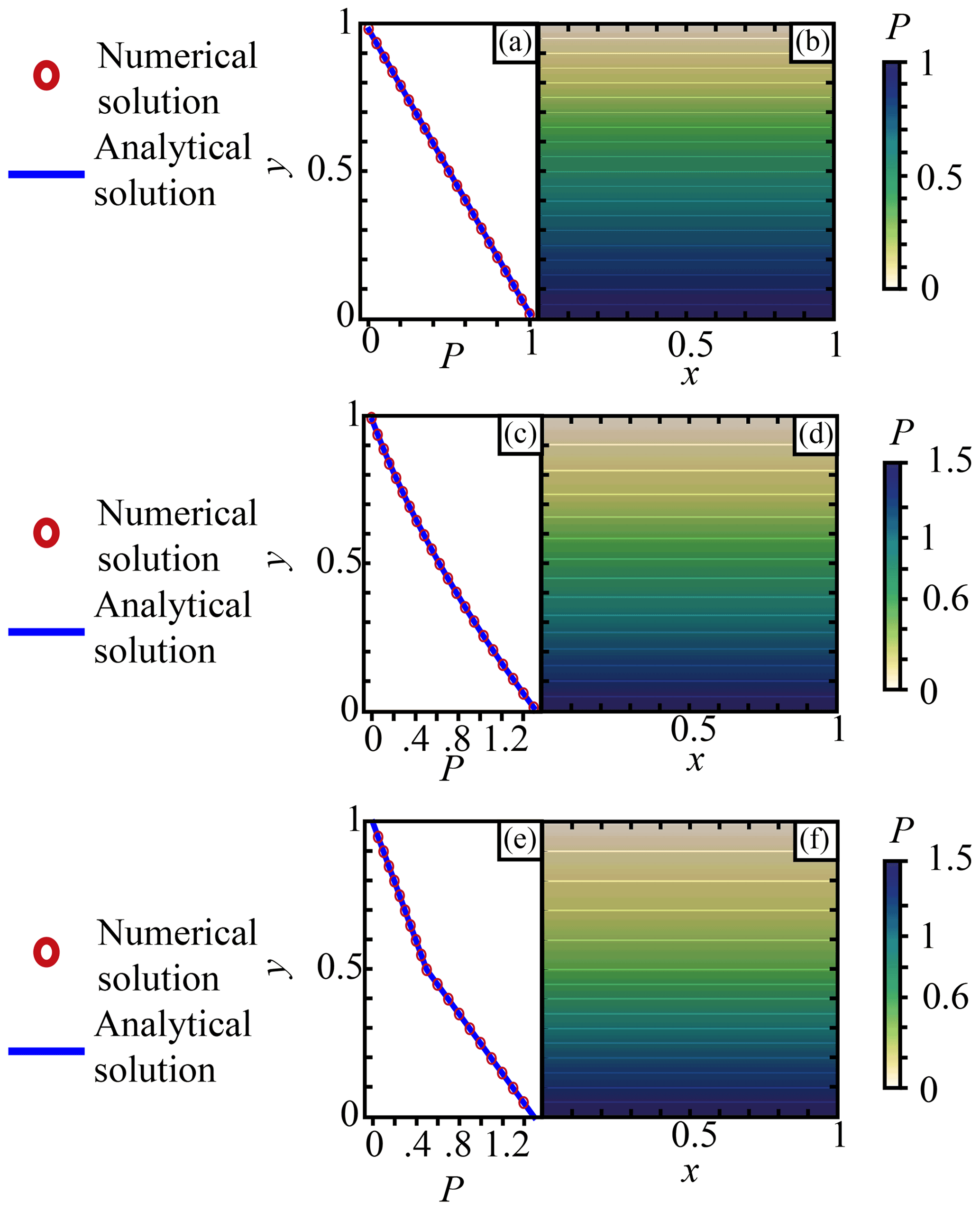
Figure 2 Pressure for non-dimensioned hydrostatic cases. Panels (a, c, e) show the 1D pressure for (a) a constant density ρ=1, (c) a continuous y-dependent density $\mathit{\rho }=\mathrm{2}-y$, and (e) a discontinuous density. The blue line is the analytical solution computed with Eq. (2), and the red circles represent the numerical solution computed with Eq. (7). Panels (b, d, f) show the 2D numerical solution for (b) a constant density ρ=1, (d) a continuous y-dependent density $\mathit{\rho }=\mathrm{2}-y$, and (f) a discontinuous density.

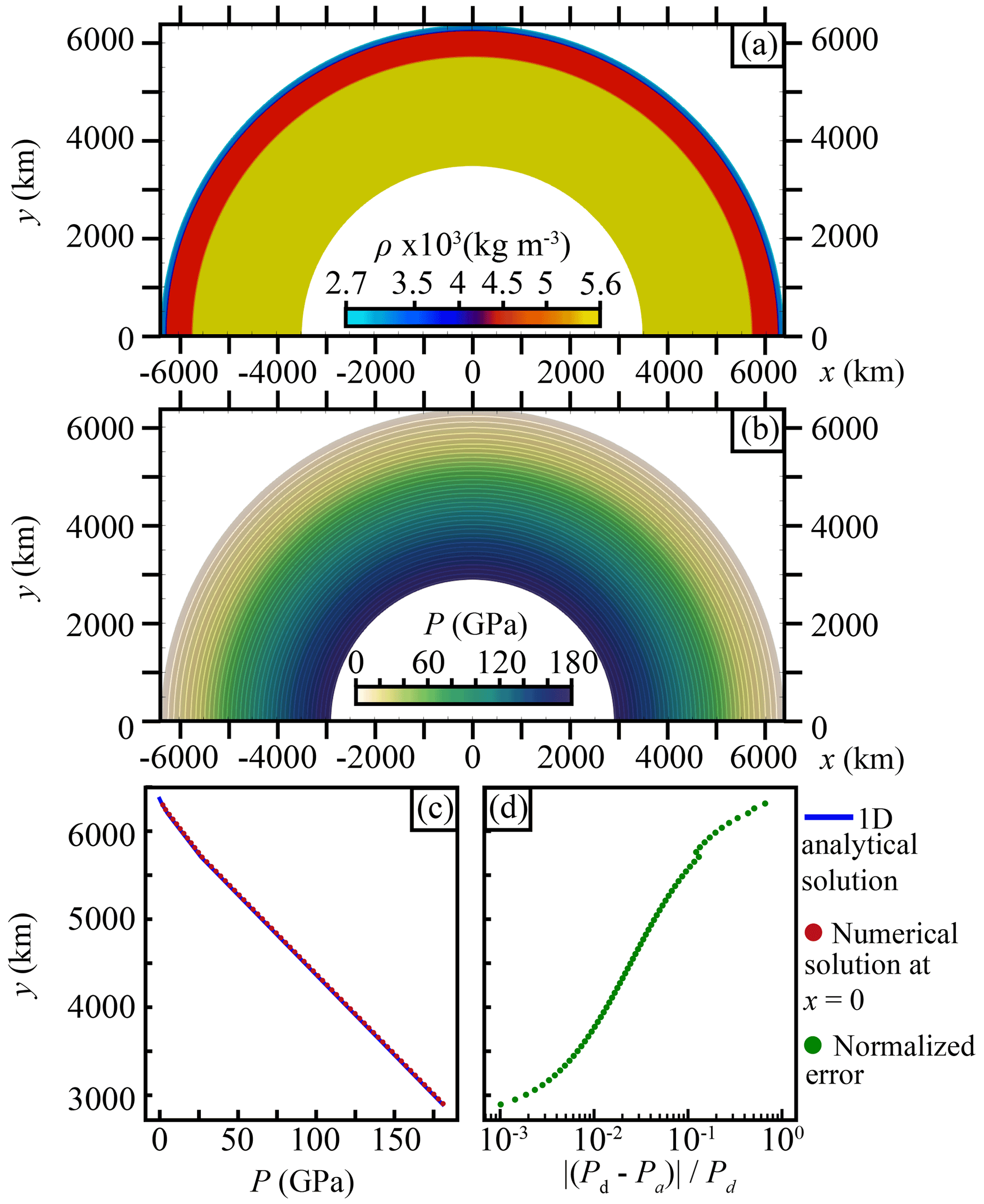
Figure 3 Pressure for a hydrostatic case in a half annulus approximating a simplified and idealized layered Earth. (a) Density structure for the half-annulus model. (b) Numerical solution of the 2D half-annulus model. (c) The blue line shows the 1D analytical solution for the density structure shown in (a) along a line parallel to the gravity vector. The red circles show the numerical solution extracted from (b) at coordinate x=0 along a line parallel to the gravity vector. (d) Green dots show the normalized error between the analytical solution and the numerical solution at x=0 as $\frac{|P_{\mathrm{d}}-P_{\mathrm{a}}|}{P_{\mathrm{d}}}$.

3.1.1 Box domain

We define the domain $\mathrm{\Omega }=x\in [\mathrm{0},\mathrm{1}]\times y\in [\mathrm{0},\mathrm{1}]$ and assume that $\mathit{g}=(\mathrm{0},-\mathrm{1})$. We consider three depth-dependent density structures ρ=ρ(y) that thus admit a hydrostatic pressure solution, i.e. satisfy $\partial P/\partial x=\mathrm{0}$, $\partial P/\partial y=-\mathit{\rho }\left(y\right)g$.

Case 1.

This case assumes a constant density, ρ(y)=1 (Fig. 2a, b). The analytic pressure solution is given by

$$\begin{array}{}\text{(29)}& \begin{array}{rl}P\left(y\right)& =\underset{y}{\overset{y_{\mathrm{s}}=\mathrm{1}}{\int }}\mathit{\rho }g\mathrm{d}y={\left[\mathit{\rho }gy\right]}_y^{y_{\mathrm{s}}}=\mathit{\rho }g(y_{\mathrm{s}}-y)\\ & =y_{\mathrm{s}}-y=\mathrm{1}-y.\end{array}\end{array}$$

Case 2.

This case assumes a continuous depth-varying density $\mathit{\rho }\left(y\right)=\mathrm{2}-y$ (Fig. 2c, d). The analytic pressure solution is given by

$$\begin{array}{}\text{(30)}& \begin{array}{rl}P\left(y\right)& =\underset{y}{\overset{y_{\mathrm{s}}=\mathrm{1}}{\int }}\mathit{\rho }g\mathrm{d}y=\underset{y}{\overset{y_{\mathrm{s}}=\mathrm{1}}{\int }}g(\mathrm{2}-y)\mathrm{d}y\\ & ={\left[g\left(-{\displaystyle \frac{\mathrm{1}}{\mathrm{2}}}{y}^{\mathrm{2}}+\mathrm{2}y\right)\right]}_y^{y_{\mathrm{s}}}\\ & =g\left({\displaystyle \frac{\mathrm{1}}{\mathrm{2}}}\left(y^{\mathrm{2}}-y_{\mathrm{s}}\right)+\mathrm{2}(y_{\mathrm{s}}-y)\right)\\ & ={\displaystyle \frac{\mathrm{1}}{\mathrm{2}}}{y}^{\mathrm{2}}-\mathrm{2}y+{\displaystyle \frac{\mathrm{3}}{\mathrm{2}}}.\end{array}\end{array}$$

Case 3.

This case assumes a discontinuous density such that ρ(y)=1 for $y\in [\mathrm{0.5},\mathrm{1}]$ and ρ(y)=2 for $y\in [\mathrm{0},\mathrm{0.5})$ (Fig. 2e, f). The analytic pressure solution is given by

$$\begin{array}{}\text{(31)}& P\left(y\right)=\left\{\begin{array}{ll}\mathit{\rho }\left(y\right)g(\mathrm{1}-y)=(\mathrm{1}-y)& \forall y\mathit{⩾}\mathrm{0.5}\\ & \\ \mathit{\rho }\left(y\mathit{⩾}\mathrm{0.5}\right)gD& \forall y<\mathrm{0.5}\\ +\mathit{\rho }\left(y\right)g(\mathrm{0.5}-y)& \\ =D+\mathrm{1}-\mathrm{2}y,& \end{array}\right.\end{array}$$

with D the distance between the surface and the y coordinate at which the pressure is computed.

A finite-element (FE) method employing an unstructured triangular mesh with a P₂ function space was used to obtain the numerical solution for each case. The FE method was applied to Eq. (27) using boundary conditions described by Eq. (15) at the base and Eq. (16) on the lateral sides. Along the upper surface we impose the Dirichlet constraint P=0. Unless otherwise stated, when solving the PPE with FEs the Dirichlet constraints are imposed strongly (i.e. point-wise), whereas Neumann constraints are imposed weakly via surface integrals defined on facets of the FE cells that live on the boundary of the domain. Accordingly, all points living on ∂Ω_surf (including corner points) will be associated with the Dirichlet constraint. Figure 2a–f shows the 1D and 2D solution of these three models. On the 1D models both the numerical and analytical solutions of Eqs. (7) and (2) are shown, whereas on the 2D models only the numerical solution is provided. Since the P₂ FE approximation contains the monomials 1, y, and y², the FE solution exactly reproduces the analytic solution for case 1 and case 2 independent of the number of finite elements used in the domain (e.g. sub-dividing the box into two triangles would be sufficient to obtain an exact solution). For case 3, the analytic pressure solution is piecewise linear, and provided that the density discontinuity is exactly resolved by the faces of the triangular FE mesh (which was the case here), the FE method exactly reproduces the analytic solution.

3.1.2 Half-annulus domain

The 2D half-annulus model aims to show the efficiency of the method when computing the lithostatic pressure in a body with a radial gravity vector and concentric density structure (Fig. 3a). This model represents a domain extending from

$$\begin{array}{}\text{(32)}& \left\{\begin{array}{ll}& \mathit{\theta }\in [-\frac{\mathit{\pi }}{\mathrm{2}},\frac{\mathit{\pi }}{\mathrm{2}}],\\ & r\in [R_{\mathrm{E}}-\mathrm{2891},R_{\mathrm{E}}]\mathrm{km},\end{array}\right.\end{array}$$

where θ is the polar angle, r is the radius in polar coordinates, R_E is the approximative Earth radius (6371 km), and R_E−2891 km is the approximative core-mantle boundary. Mapped into Cartesian coordinates this gives x=rsin (θ) and y=rcos (θ). The gravity vector pointing to the centre ($\mathit{x}=(\mathrm{0},\mathrm{0})$) is defined as $\mathit{g}=-\mathrm{9.8}\left(\frac{x}{\sqrt{x^{\mathrm{2}}+y^{\mathrm{2}}}},\frac{y}{\sqrt{x^{\mathrm{2}}+y^{\mathrm{2}}}}\right)$ m s⁻², and the density is defined as five concentric layers with a constant density in each (Fig. 3a). The pressure was computed by solving Eq. (27) with the boundary condition of Eq. (15) on the core–mantle boundary and the conditions of Eq. (16) on the sides parallel to $\widehat{\mathit{g}}$. At the surface of the domain we impose the Dirichlet constraint P=0. As in Sect. 3.1 we use a finite-element discretization employing an unstructured mesh of triangles employing a P₂ function space. Pressure values vary from 0 to 180 GPa with a concentric distribution following the density distribution and the gravity vector orientation (Fig. 3b).

The numerical solution extracted at x=0 along a line parallel to the gravity vector field reproduces the analytical solution computed for a 1D profile using Eq. (2) for the density distribution displayed in the half-annulus model (Fig. 3c). The difference between the pressure obtained using the depth-integrated approach and the PPE is very small (Fig. 3d). Unlike the analytic solution for the box models, the analytic solution for P here is non-polynomial (in Cartesian coordinates); hence, the FE solution (which was discretized in Cartesian coordinates) cannot exactly reproduce the analytic solution.

The four hydrostatic models clearly illustrate that the solutions obtained using the depth-integrated approach and the pressure Poisson equation (with one set of boundary constraints) are equivalent for scenarios that admit a hydrostatic solution.

3.2 Non-hydrostatic pressure

Here, we show the differences and accuracy of the depth-integrated equation (Eq. 2) and the pressure Poisson equation (Eq. 7) approaches to approximate the total pressure. First, we compute and compare the pressure from the different methods in a large domain (referred to as the “global” model) containing a topographic perturbation (Fig. 4). Following this, we compute the pressure in a smaller domain (referred to as the “regional” model) and show the accuracy of the different methods to approximate the total pressure from the large domain (Figs. 5a, c and 6). Finally, we show the velocity field resulting from applying these approximated pressures as boundary conditions to solve the conservation of momentum in the small domain (Fig. 5b, d). The pressure Poisson problem was discretized and solved using the same FE method described in Sect. 3.1. The flow field was computed using the same underlying FE mesh and a mixed P₂-P₁ function space for velocity and pressure, respectively.

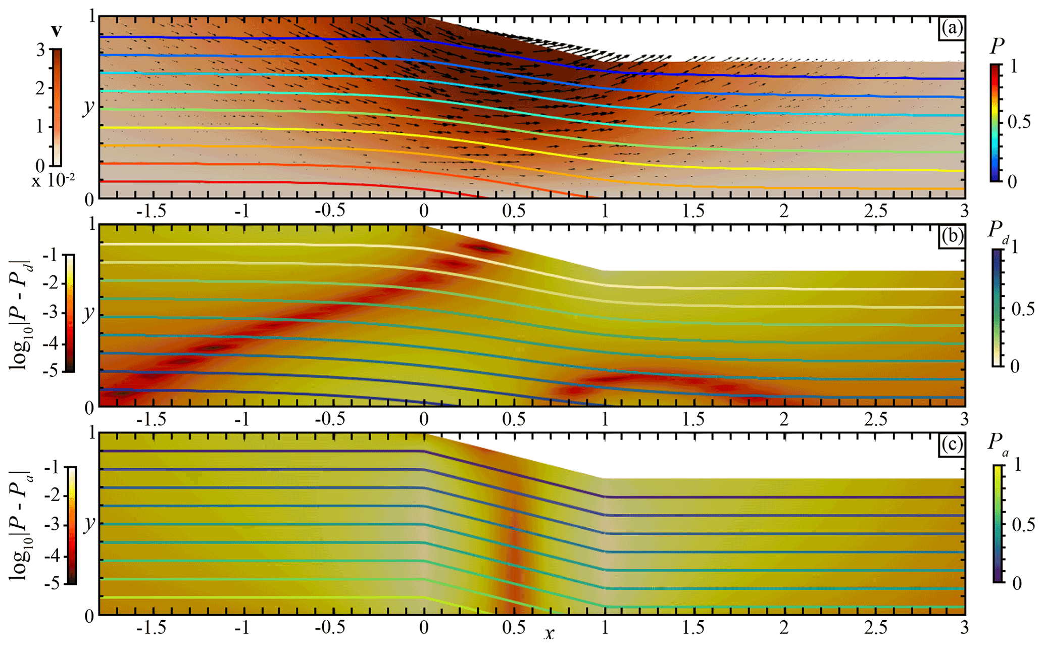
Figure 4 Non-dimensional “global” model for a large domain with a topographic perturbation. (a) The background colour shows the velocity field computed with the Eq. (3). The coloured curves show the total pressure P iso-values every 0.1 computed with Eq. (3). (b) Comparison between the total pressure from Eq. (3) and the pressure P_d computed from Eq. (7). The coloured background shows the difference ${\log }_{\mathrm{10}}|P-P_{\mathrm{d}}|$. The coloured curves show the pressure P_d iso-values every 0.1 computed with Eq. (7). (c) Comparison between the total pressure from Eq. (3) and the pressure P_a computed from Eq. (2). The coloured background shows the difference ${\log }_{\mathrm{10}}|P-P_{\mathrm{a}}|$. The coloured curves show the pressure P_a iso-values every 0.1 computed with Eq. (2).

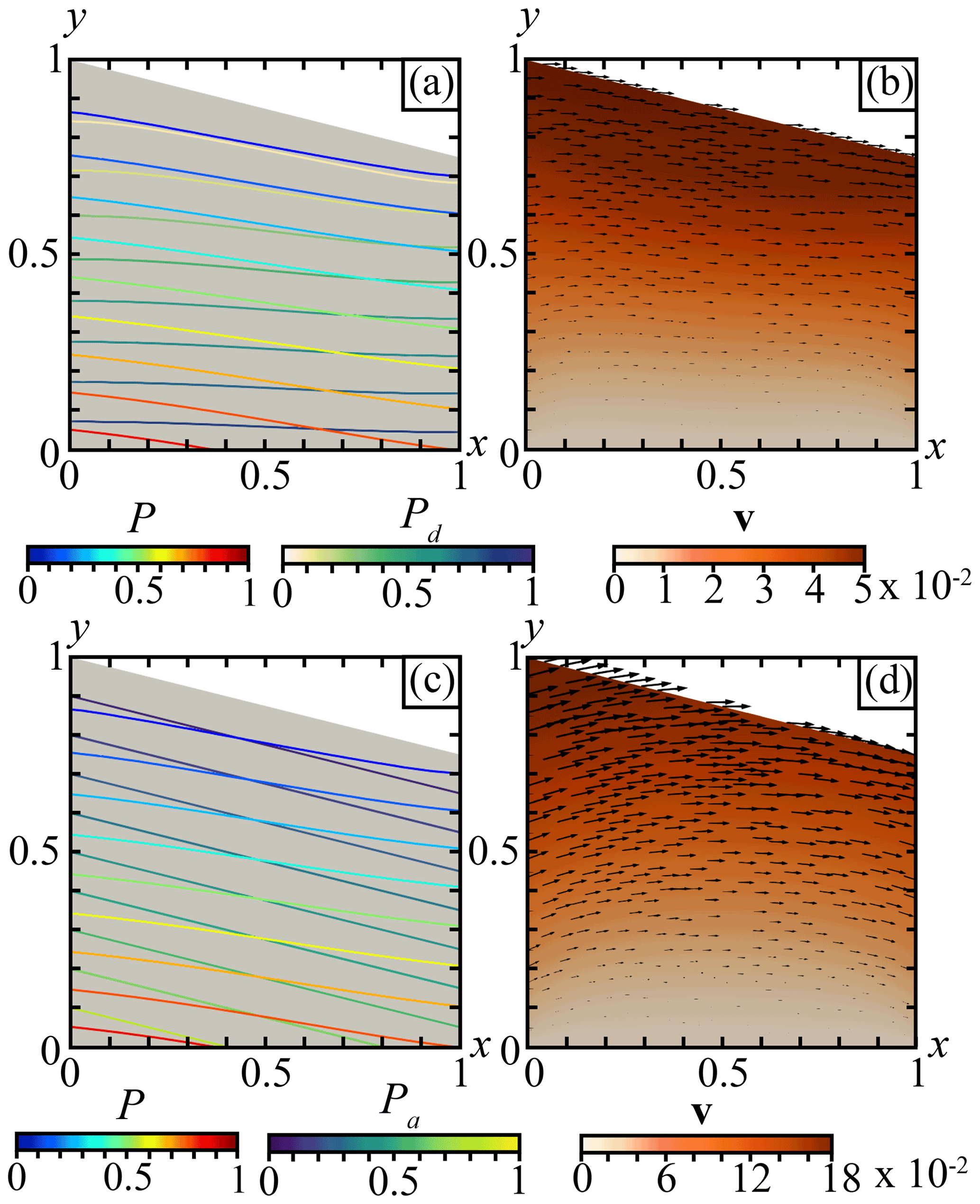
Figure 5 Non-dimensional “regional” model for a small domain with a varying topography. (a) The coloured curves show the total pressure P iso-values computed with Eq. (3) in the global model every 0.1 and the pressure P_d computed with Eq. (7) in the regional model every 0.1. (b) The coloured background shows the velocity field computed with Eq. (3) with stress boundary conditions described by Eq. (33) using P_d computed with Eq. (7). The black arrows show the velocity vectors. (c) The coloured curves show the total pressure P iso-values computed with Eq. (3) in the global model every 0.1 and the pressure P_a computed with Eq. (2) in the regional model every 0.1. (d) The coloured background shows the velocity field computed with Eq. (3) with stress boundary conditions described by Eq. (33) using P_a computed with Eq. (2). The black arrows show the velocity vectors.

3.2.1 “Global” model

We define a large domain ${\mathrm{\Omega }}_{\mathrm{G}}=x\in [-\mathrm{10},\mathrm{10}]\times y\in [\mathrm{0},\mathrm{1}]$ representing a global model, i.e. 20 times larger than the domain of interest, in order to avoid boundary condition influence (Fig. 4). In this domain, we introduce a topographic perturbation through a slope defined as $y_{\mathrm{s}}\left(x\right)=-\frac{\mathrm{1}}{\mathrm{4}}x$, where y_s is the surface between x=0 and x=1. For demonstration purposes this topography is highly exaggerated with respect to the depth of the domain compared with the actual regional geodynamic models. Moreover, we use a constant density ρ=1 and a vertical gravity vector $\mathit{g}=(\mathrm{0},-\mathrm{1})$.

We solve the flow problem described by Eqs. (3), (4) using a constant viscosity and density, along with the following boundary conditions: no-slip at base, free-slip on the right and left faces, and a free surface along the top of the model domain. Due to the topography, a non-vertical pressure gradient that will drive flow is generated below that perturbation (Fig. 4a). The generated flow shows a velocity field characteristic of a gravitational collapse. Figure 4b shows the difference between the total pressure solution from Eq. (3) with the pressure P_d obtained by solving Eq. (7) using the boundary conditions described by Eq. (16) on the vertical sides, Eq. (15) on the bottom boundary, and P_d=0 on the upper surface. Figure 4c shows the difference with the pressure P_a obtained with Eq. (2).

The difference between the total pressure and the approximated pressure P_d is negligible in the non-perturbed domain and increases with the topography perturbation. It shows that as the system tends towards a hydrostatic state the total pressure and the approximated pressure P_d tends to the same value, i.e. the hydrostatic pressure. However, in the vicinity of the topographic perturbation the differences between the total pressure and the approximated pressure can be extremely small (Fig. 4b). In contrast, the difference between the total pressure and depth-integrated approximated pressure P_a is larger below the topographic slope, particularly below the points at which the slope begins and ends (Fig. 4c). In general, the pressure P_a obtained by applying the 1D solution is less accurate than P_d within both the interior and along the left, right, and bottom boundaries.

3.2.2 “Regional” model

Nevertheless, modelling a domain 20 times larger than the domain of interest can hardly be achieved in practice, mainly due to the numerical cost it represents. Thus, the boundary conditions are a first-order component of regional models in order to best capture the global behaviour and interactions in a region without having to model the whole Earth. Therefore, we define a smaller domain ${\mathrm{\Omega }}_R=x\in [\mathrm{0},\mathrm{1}]\times y\in [\mathrm{0},\mathrm{1}]$ representing a regional model (Fig. 5). This domain represents the portion of the large domain in which the topographic slope is defined.

In this case we aim to apply a normal stress on the boundaries of our regional model that will generate a flow similar (or close) to the flow generated in the global model. To achieve this we present two models using Eqs. (7) and (2), respectively, to compute an approximated pressure that is then used as a boundary condition for the momentum equation (Eq. 3) on vertical boundaries as follows:

$$\begin{array}{}\text{(33)}& \mathit{\sigma }\mathit{n}=-P_{\mathit{\alpha }}\widehat{\mathit{n}},\mathit{\alpha }=\mathrm{d},\mathrm{a},\end{array}$$

where $P_{\mathit{\alpha }}=\mathit{\{}{P}_{\mathrm{d}},P_{\mathrm{a}}\mathit{\}}$ denote the pressure computed using the pressure Poisson equation and the 1D depth-integrated approach, respectively. The viscous flow problem for the regional domain setting employs the following additional boundary conditions: a free surface on the top boundary and a no-slip condition at the base. To solve for the pressure P_d using Eq. (7), we impose the following boundary conditions: P_d=0 on the surface, $\mathrm{\nabla }{P}_{\mathrm{d}}\cdot \widehat{\mathit{n}}=(\widehat{\mathit{n}}\cdot \widehat{\mathit{g}})\mathrm{\nabla }{P}_{\mathrm{d}}\cdot \widehat{\mathit{g}}$ on vertical sides, and $\mathrm{\nabla }{P}_{\mathrm{d}}\cdot \widehat{\mathit{n}}=(\widehat{\mathit{n}}\cdot \widehat{\mathit{g}})\mathit{\rho }g+(\widehat{\mathit{n}}\cdot \widehat{{\mathit{g}}_{⟂}})\mathrm{\nabla }{P}_{\mathrm{d}}\cdot \widehat{{\mathit{g}}_{⟂}}$ at the bottom.

Figure 5a shows the pressure field P_d computed on the regional domain and the total pressure P extracted from the global model. The approximated pressure P_d highlights differences with the total pressure from the global model, especially those regarding depth along the boundaries (blue lines in Fig. 6b, d). These differences are mainly due to the size of the domain that defines only the perturbed region without providing information about the domain in which it is enclosed. The boundary condition described by Eq. (16) used to solve Eq. (7) enforces the idea that the pressure gradient must be co-linear with the gravity vector on the boundary. Therefore, given the definition of g, ∇P is enforced to be vertical on the vertical sides, whereas the deflection of the pressure field due to the topographic perturbation should occur in spatial offset from the topographic perturbation, as shown by the total pressure in the global model (Fig. 4a).

In Fig. 5b we show the velocity field resulting from solving the Stokes equation (Eqs. 3, 4) using P_d in Eq. (33). The flow field highlights velocities of around $\mathrm{5}\times {\mathrm{10}}^{-\mathrm{2}}$ (velocity unit) at the surface pointing toward the right side of the domain, i.e. the bottom of the slope. Velocities progressively decrease at depth. While the orientation of the velocity field is more laminar than in the global model, its magnitude is very close, with the highest velocities being only 1.5× higher than in the global model.

Figure 5c displays the pressure field P_a computed from the depth-integrated approach (Eq. 2) within the regional domain and the total pressure P extracted from the global model. Because of the 1D behaviour of that method, the differences between the approximated pressure P_a and the total pressure P (red lines in Figs. 5c and 6b, d) are independent of the domain size and boundary conditions, and thus they are exactly the same as in the global model (Fig. 4c). The velocity field (Fig. 5d) resulting from using these approximated pressure values as a boundary condition to solve the momentum equation is approximatively 4 times higher than velocities obtained while using the pressure P_d (Fig. 5b) and approximatively 6 times higher than in the global model (Fig. 4a). As for the velocity field orientation, the vectors at the top of the slope show that the material uplifts, whereas in the global model velocities at the same location show a gravitational sliding. This orientation results from a stress value that is too high being imposed in the boundary conditions by the value of the pressure P_a at the boundaries (Fig. 6).

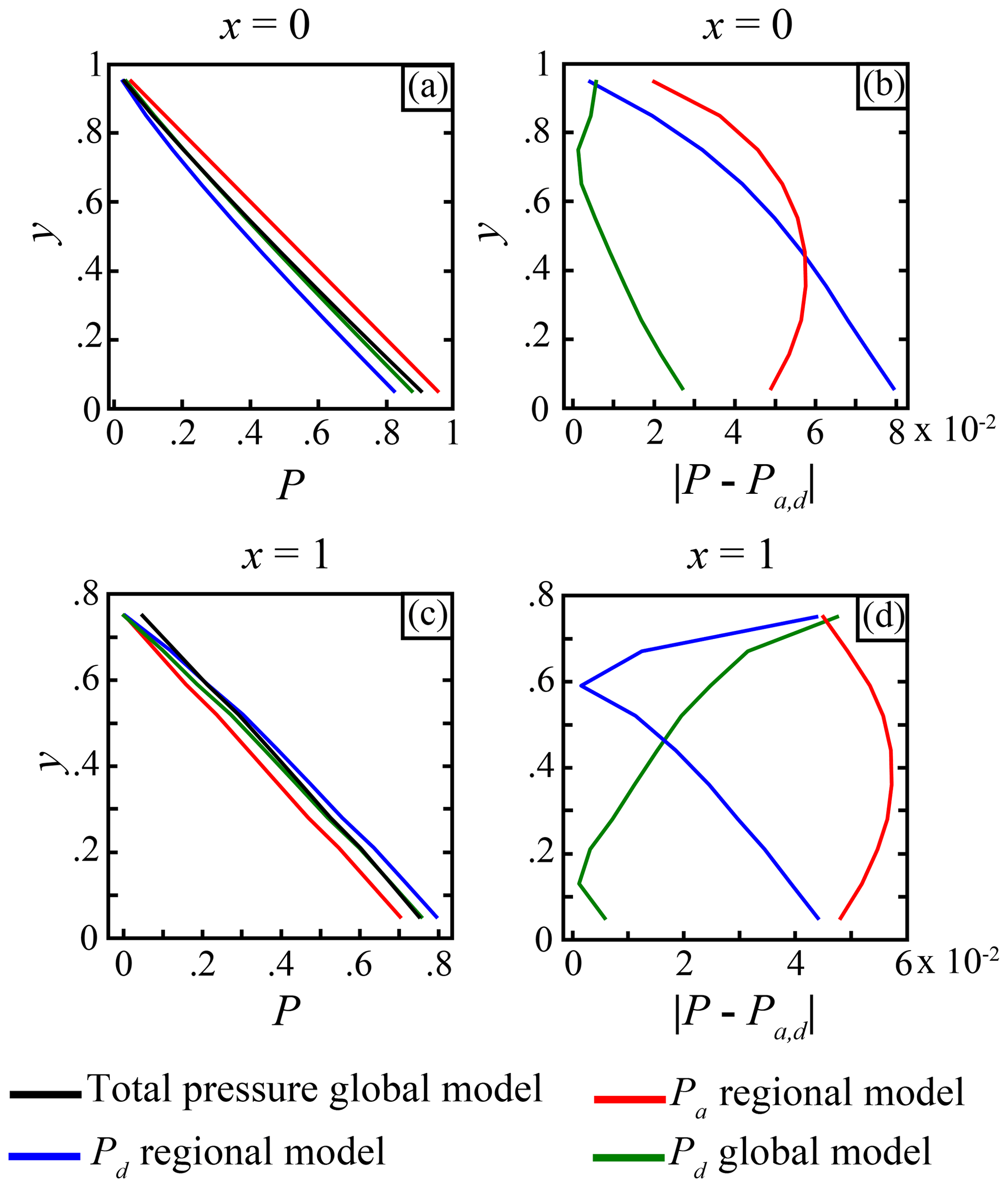
Figure 6 Curves showing the pressure from the regional and global models along the profiles (a) x=0 and (c) x=1. Absolute value of the difference between the total pressure P in the global model and the different pressures in the global and regional models along the profiles (b) x=0 and (d) x=1.

These simple tests demonstrate that the approximated pressure P_d computed from the Eq. (7) is more accurate for approximating the total pressure P than the pressure P_a computed from the Eq. (2). The only area where this is not true is located in the bottom-left corner of the regional model, and this is again due to the boundary condition not capturing the deflection of the pressure due to the size of the domain. Thus, the pressure computed with the pressure Poisson problem should be preferred for use as a boundary condition for the momentum equation. Moreover, as the domain size increases the error with the total pressure decreases, which is not the case with the depth-integrated approach due to its 1D nature.

3.3 Influence of the boundary condition type

The boundary conditions used to solve the pressure Poisson problem are stated in Eqs. (15), (16), and (23). To show the influence of the boundary conditions choices on the resulting pressure field, we define an irregular quadrilateral domain with the same topographic perturbation as the one described in Sect. 3.2, with a constant density ρ=1, a gravity vector $\mathit{g}=(\mathrm{0},-\mathrm{1})$, and a Dirichlet boundary condition P_d=0 at the top surface (Γ_s). The irregular domain (shown in Fig. 7) is constructed such that none of the three boundary segments defining $\partial {\mathrm{\Omega }}_i={\mathrm{\Gamma }}_{\mathrm{1}}\cup {\mathrm{\Gamma }}_{\mathrm{2}}\cup {\mathrm{\Gamma }}_{\mathrm{3}}$ are parallel or perpendicular to g. The PPE was solved using the same FE method described in Sect. 3.1.

Figure 7 Pressure field P_d computed using Eq. (7) for different boundary conditions applied to the individual boundary segments ${\mathrm{\Gamma }}_i,i=\mathrm{1},\mathrm{2},\mathrm{3}$. The boundary conditions were defined according to (a) Eq. (15) on Γ₁, Γ₂, and Γ₃; (b) Eq. (15) on Γ₁ and Γ₂ and Eq. (16) on Γ₃; (c) Eq. (15) on Γ₂ and Eq. (16) on Γ₁ and Γ₃; and (d) Eq. (15) on Γ₃ and Eq. (16) on Γ₁ and Γ₂.

In Fig. 7 we show different pressure fields P_d obtained using several different boundary condition configurations. These results show that the boundary conditions described by Eq. (16) (or Eq. 20) force the pressure gradient to be parallel to g, i.e. ${\partial }_x{P}_{\mathrm{d}}=\mathrm{0}$ (Fig. 7b segment Γ₃, Fig. 7c segments Γ_1,3, and Fig. 7d segments Γ_1,2). We also confirm that boundary conditions described by Eq. (15) (or Eq. 19) constrain ∇P_d to be equivalent to the 1D solution of Eq. (2) on the boundary (Fig. 7a segments ${\mathrm{\Gamma }}_{\mathrm{1},\mathrm{2},\mathrm{3}}$, Fig. 7b segments Γ_1,2, Fig. 7c segment Γ₂, and Fig. 7d segment Γ₃). Figure 7a highlights that the solution of the PPE can be identical to that obtained using the depth-integrated approach with a specific choice of boundary conditions.

Moreover, Fig. 8a shows the pressure field P_d obtained using the boundary condition described by Eq. (23). The pressure solution is relatively similar to the solution obtained in Fig. 7c. However, as shown in Fig. 8b, the solution along the boundary (and therefore also in the interior) differs since Eq. (23) does not enforce the pressure gradient to be vertical on the boundary compared with the condition (16).

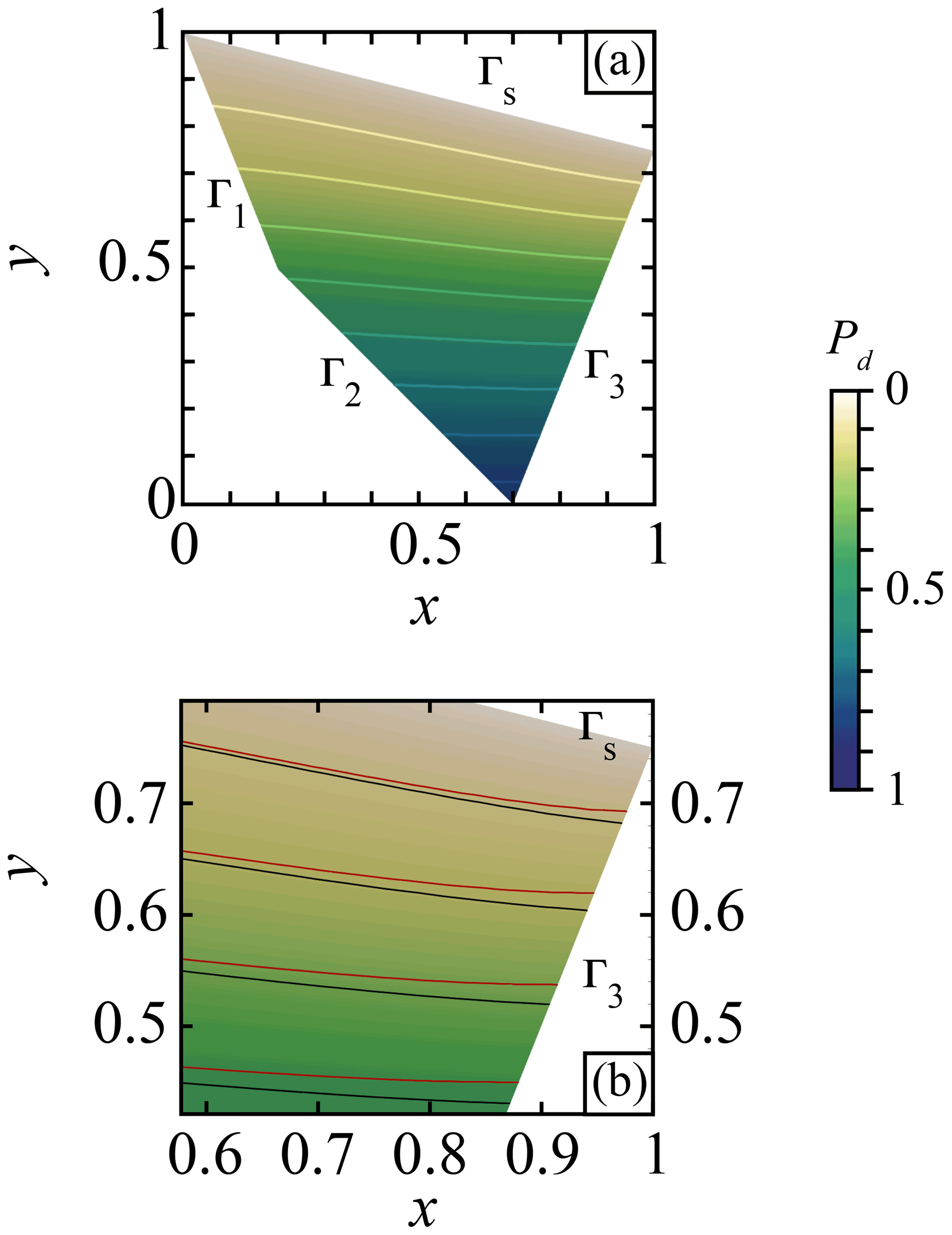
Figure 8 Pressure field P_d computed using Eq. (7) with the boundary conditions described by Eq. (23) for (a) P_d over the entire model with boundary conditions defined by Eq. (23) applied on Γ₁, Γ₂, and Γ₃. (b) Closer view of the right-hand boundary region. The black curves show the iso-values of the pressure computed with boundary conditions using Eq. (23). The red curves show the iso-values of the pressure computed using the boundary conditions used in Fig. 7c.

As previously noted, discretizations employing the weak form with Eq. (23) are certainly simpler to implement than imposing the Eqs. (19) and (20) as all the surface integrals cancel (see Eq. 28), and thus no surface integrals appear in either the linear form or bilinear form. We also reiterate that when the domain has boundaries that are aligned with g, using the boundary conditions (15) on the boundaries orthogonal to g and the condition (16) on the boundaries that are parallel to g results in an identical formulation.

3.4 Thermo-mechanical model

3.4.1 Physical model

To simulate the long-term evolution of the deformation of the lithosphere, we solve the stationary, non-inertial form of the conservation of momentum described by Eq. (3) with the incompressible constraint (Eq. 4). Moreover, to consider the temperature variations in the domain, the following time-dependent conservation of energy is solved:

$$\begin{array}{}\text{(34)}& {\mathit{\rho }}_{\mathrm{0}}{C}_p\left({\displaystyle \frac{\partial T}{\partial t}}+\mathit{v}\cdot \mathrm{\nabla }T\right)=\mathrm{\nabla }\cdot \left(k\mathrm{\nabla }T\right)+H,\end{array}$$

where T is the temperature, t is the time, k is the thermal conductivity, H is the heat source, ρ₀ is the reference density, and C_p the thermal heat capacity.

The numerical solution of Eqs. (3) and (4) is obtained using a mixed finite-element method that independently discretizes the velocity and pressure fields. Hence, the numerical velocity and pressure obtained are solutions of the weak form of the Stokes problem given by

$$\begin{array}{rl}& \mathcal{A}(\mathit{w},\mathit{v})+\mathcal{B}(\mathit{w},p)+\mathcal{B}(\mathit{v},q)-\underset{{\mathrm{\Gamma }}_{\mathrm{N}}}{\int }\mathit{w}\cdot \mathit{T}(\mathit{v},p)\mathrm{d}S\\ & =-\underset{\mathrm{\Omega }}{\int }\mathit{\rho }\mathit{w}\cdot \mathit{g}\mathrm{d}V\end{array}$$

where w∈H₁(Ω) and q∈L₂(Ω) are test functions for the velocity and pressure, respectively, Γ_N denotes the Neumann boundary, T denotes the traction vector given by $\mathit{T}(\mathit{v},p)=\left(\mathit{\tau }\right(\mathit{u})-p\mathbb{I})\widehat{\mathit{n}}$, and $\widehat{\mathit{n}}$ is the outward pointing normal vector from the boundary. The bilinear forms for the Stokes problem are given by (Elman et al., 2014):

$$\begin{array}{c}{\displaystyle }\mathcal{A}(\mathit{w},\mathit{v})=\underset{\mathrm{\Omega }}{\int }\mathrm{2}\mathit{\eta }\dot{\mathit{\epsilon }}\left(\mathit{w}\right):\dot{\mathit{\epsilon }}\left(\mathit{v}\right)\mathrm{d}V,\dot{\mathit{\epsilon }}\left(\mathit{v}\right)=\frac{\mathrm{1}}{\mathrm{2}}[\mathrm{\nabla }\mathit{v}+(\mathrm{\nabla }\mathit{v}{)}^T],\\ {\displaystyle }\mathcal{B}(\mathit{v},q)=-\underset{\mathrm{\Omega }}{\int }q\mathrm{\nabla }\cdot \mathit{v}\mathrm{d}V.\end{array}$$

Both the Stokes and thermal problems were solved using the parallel finite-element code pTatin3D (May et al., 2014, 2015), which employs a mixed Q₂-P₁ discretization for velocity and pressure.

3.4.2 Initial conditions and rheology

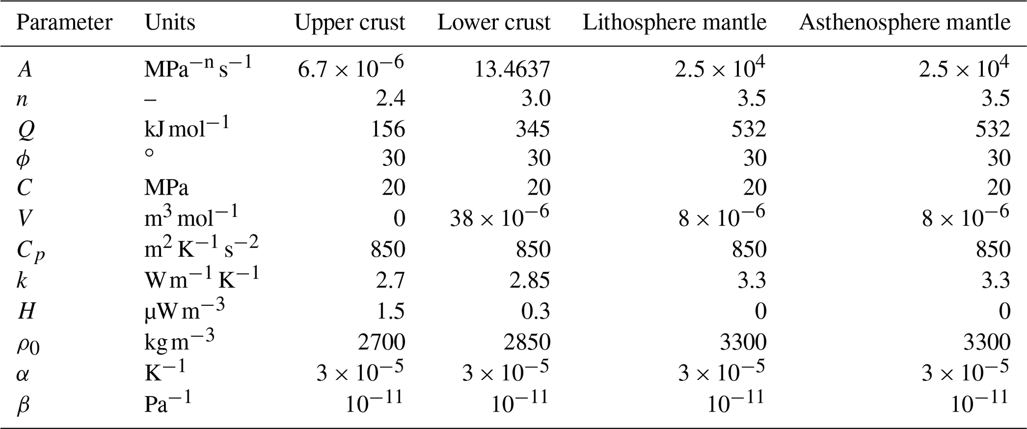
To model the strain localization we use non-linear visco-plastic rheologies expressed in term of viscosity. The ductile parts of the domain are simulated using an Arrhenius flow law for dislocation creep

$$\begin{array}{}\text{(35)}& {\mathit{\eta }}_v=A^{-\frac{\mathrm{1}}{n}}{\left({\dot{\mathit{\epsilon }}}^{\mathrm{II}}\right)}^{\frac{\mathrm{1}}{n}-\mathrm{1}}\exp \left({\displaystyle \frac{Q+PV}{nRT}}\right),\end{array}$$

where A, Q, and n are material-defined parameters (see Table 1); R is the universal gas constant; V is the activation volume; and ${\dot{\mathit{\epsilon }}}^{\mathrm{II}}$ is the square root of the strain rate second invariant, computed as

$$\begin{array}{}\text{(36)}& {\dot{\mathit{\epsilon }}}^{\mathrm{II}}=\sqrt{{\displaystyle \frac{\mathrm{1}}{\mathrm{2}}}{\dot{\mathit{\epsilon }}}_{ij}{\dot{\mathit{\epsilon }}}_{ij}}.\end{array}$$

The brittle parts of the domain are simulated using a Drucker–Prager yield criterion adapted to continuum mechanics, which is given by

$$\begin{array}{}\text{(37)}& {\mathit{\eta }}_p={\displaystyle \frac{C\cos \left(\mathit{\varphi }\right)+P\sin \left(\mathit{\varphi }\right)}{\mathrm{2}{\dot{\mathit{\epsilon }}}^{\mathrm{II}}}},\end{array}$$

where C is the cohesion of the material and ϕ is the friction angle.

The modelled domain contains four initial flat layers representing the upper continental crust, the lower continental crust, the lithosphere mantle, and the asthenosphere mantle, respectively (Fig. 9a). The upper crust extends from the surface of the domain (y=0 km) to $y=-\mathrm{25}$ km and is modelled with a dislocation creep quartz rheology (Ranalli, 1997). The lower crust extends from $y<-\mathrm{25}$ km to $y=-\mathrm{35}$ km and is modelled with a dislocation creep anorthite rheology (Rybacki and Dresen, 2000). The lithosphere mantle extends from $y<-\mathrm{35}$ km to $y=-\mathrm{120}$ km, whereas the asthenosphere mantle extends from $y<-\mathrm{120}$ km to $y=-\mathrm{450}$ km. They are both modelled using a dislocation creep olivine flow law (Hirth and Kohlstedt, 2003).

Figure 9 (a) A 3D view of the modelled domain. An initial plastic strain with a Gaussian repartition is applied in the central part of the domain in the lithosphere. (b) Map and cross section of the boundary conditions for the model with free-slip boundary conditions. (c) Map and cross section of the boundary conditions for the model with normal stress boundary conditions. (d) Yield–stress envelope and initial temperature of the first 120 km.

The initial density distribution follows the lithologies and is reported in Table 1. In addition, the density varies with pressure and temperature following the Boussinesq approximation

$$\begin{array}{}\text{(38)}& \mathit{\rho }(P,T)={\mathit{\rho }}_{\mathrm{0}}(\mathrm{1}-\mathit{\alpha }(T-T_{\mathrm{0}})+\mathit{\beta }(P-P_{\mathrm{0}}\left)\right),\end{array}$$

where ρ₀ is the reference density at T₀ and P₀, P is the total pressure computed from the conservation of momentum (Eq. 3) and continuity equation (Eq. 4), α is the thermal expansion and β the compressibility. The Boussinesq approximation states that perturbations of density, if sufficiently small, can only be considered in the buoyancy term and neglected elsewhere regardless of the origin of the perturbation.

Moreover, the initial temperature field is computed as a steady-state solution of the heat equation

$$\begin{array}{}\text{(39)}& \mathrm{\nabla }\cdot \left(k\mathrm{\nabla }T\right)+H=\mathrm{0},\end{array}$$

using a surface temperature of T=0 ^∘C at y=0 km and T=1450 ^∘C at $y=-\mathrm{450}$ km. Moreover, to simulate an adiabatic thermal gradient in the asthenosphere due to thermal convection, the initial temperature field is solved with a conductivity of k=70 W m⁻¹ K⁻¹ in the asthenospheric mantle. However, for the actual model run we used a more realistic conductivity of k=3.3 W m⁻¹ K⁻¹ to solve Eq. (34). Other thermal parameters are reported in Table 1.

Table 1 Physical parameters for the thermo-mechanical rift model.

3.4.3 Boundary conditions

To show the influence of the normal stress boundary condition, we compare two rift models. In the reference model, an extension velocity of v_x=1 cm yr⁻¹ is applied on the whole faces of normal x, whereas on faces of normal z a free-slip boundary condition is applied (Fig. 9c). To ensure mass conservation we impose an inflow velocity on the bottom face of normal y to balance any outflow that occurs due to the imposed extension. Along the surface of the model we use a free surface (zero normal stress, zero tangential stress) boundary condition.

The second rift model (Fig. 9b) uses the same Dirichlet boundary conditions on faces of normal x. On the faces of normal z we impose a Neumann boundary condition as

$$\begin{array}{}\text{(40)}& \mathit{T}=-P_{\mathrm{d}}\widehat{\mathit{n}},\end{array}$$

where P_d is the pressure computed with Eq. (7) and $\widehat{\mathit{n}}$ is the normal vector pointing outward from the domain.

To account for the density evolution through time due to the deformation and material advection, Eq. (7) is solved at every non-linear iteration for each time step, and the Neumann boundary condition described by Eq. (40) is evaluated at every non-linear iteration. Using ρ(P,T) computed from Eq. (38) to evaluate the pressure P_d going into the boundary condition described by Eq. (40) adds a new non-linearity to the system.

The bottom of the domain is prescribed as an inflow condition balancing the outflow, and the surface of the domain is a free surface where the mesh deforms according to the computed velocity field. These Neumann boundary conditions allow material to flow both in and out through the boundary depending only on the Dirichlet boundary conditions and deformation that occurs inside the modelled domain.

3.4.4 Pressure Poisson problem in the 3D geodynamic model

In the context of our finite-element forward model, we also solve the pressure Poisson problem using finite elements. As such, to compute P_d we employ the weak formulation given by Eq. (27) using boundary conditions from Eqs. (15) and (16) on bottom boundary and vertical boundaries, respectively. In our particular implementation, we employ Q₁ for P_d, and these Q₁ elements overlap the Q₂ elements used to approximate the velocity.

As a demonstration of the computed P_d using this approach, in Fig. 10c and d we show the approximated pressure in our rift model at 8.7 Myr after large deformations that led to mantle exhumation and differential thinning of the continental crust, causing a variable topography. In this model, P_d was evaluated on a mesh consisting of $\mathrm{256}\times \mathrm{64}\times \mathrm{128}{Q}_{\mathrm{1}}$ finite elements on 1024 MPI ranks. The discrete pressure Poisson system was solved using geometric multigrid. As a rough estimate, solving for P_d required ∼0.2 % of the time required to solve the non-linear viscous flow problem. Obviously this value is strongly dependent on both the physical model (linear viscous versus non-linear viscous) and the implementation details, as well as the efficiency of how the discrete flow problem is solved. However, when considering even the simplest flow problem imaginable (i.e. linear iso-viscous flow laws), it remains true that solving the Poisson problem will be far less expensive than solving either the linear or non-linear viscous flow problem.

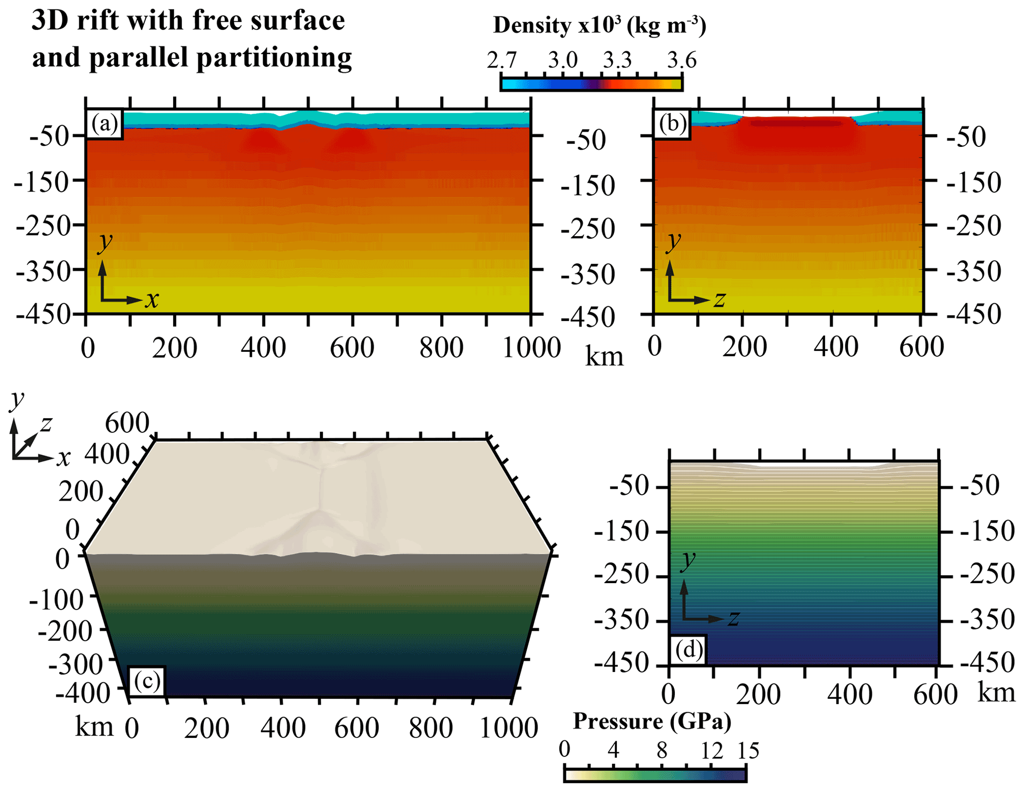
Figure 10 (a) Cross section showing the density of the 3D rift model with normal stress boundary conditions in the x–y plane at z=0. (b) Cross section showing the density of the z–y plane at x=500 km. (c) 3D view of the pressure computed with Eq. (7). (d) Cross section of the z–y plane at x=500 km for the reference pressure. The contour lines are plotted every 0.25 GPa.

3.4.5 Tectonics evolution

The model using free-slip boundary conditions displays a cylindrical deformation pattern that could be reduced to a two-dimensional model. As shown by the shear zone orientation and strain regime, the deformation is only extensional and perpendicular to the extension direction (Figs. 11a–d and 12). This strain localization is directly due to the free-slip boundary condition stating that any flow perpendicular to the boundary is prohibited.

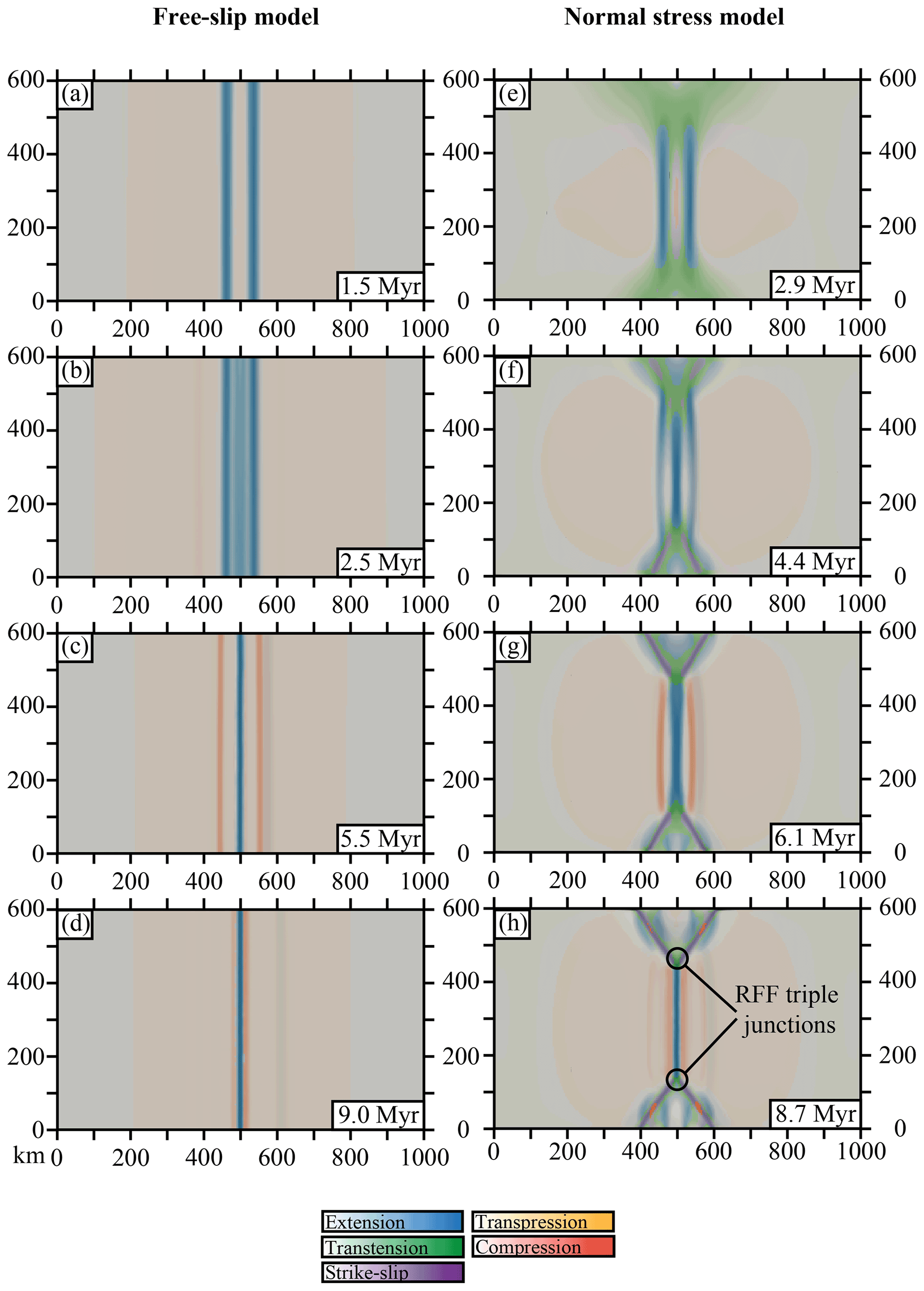
Figure 11 Map view of the strain regime evolution in time and space of the model with (a–d) free-slip boundary conditions and (e–h) normal stress boundary conditions.

Figure 12 Map view of the models with free-slip (left) and normal stress (right) boundary conditions. The dashed lines in the upper panels indicated by (a–a^′, b–b^′, c–c^′) correspond to the cross sections displayed in the lower panels with the same labelling. The cross sections show the numerical lithologies with the second invariant of the strain rate (Eq. 36) and the strain regime.

In contrast, the model using the P_d pressure as a boundary condition displays a non-cylindrical deformation. While extensional shear zones perpendicular to the extension direction develop in the central part of the domain, the edges of the rift experience oblique and strike-slip deformation (Fig. 11e to h). As the extension goes on, the extensional deformation localizes along a spreading centre, causing an increasing inflow on the boundaries of the domain with the normal stress boundary condition (Fig. 13c). As a result, near these boundaries the velocity field introduces non-cylindrical features that are accommodated by strike-slip faults (Fig. 11g, h). These strike-slip faults delimit a triangular region terminating on a triple junction between two strike-slip faults and a ridge (ridge–fault–fault, RFF, triple junction). Along these strike-slip faults, the deformation is partitioned between purely vertical strike-slip shear zones and shallow-dipping normal shear zones rooting into the strike-slip shear zones (Fig. 12).

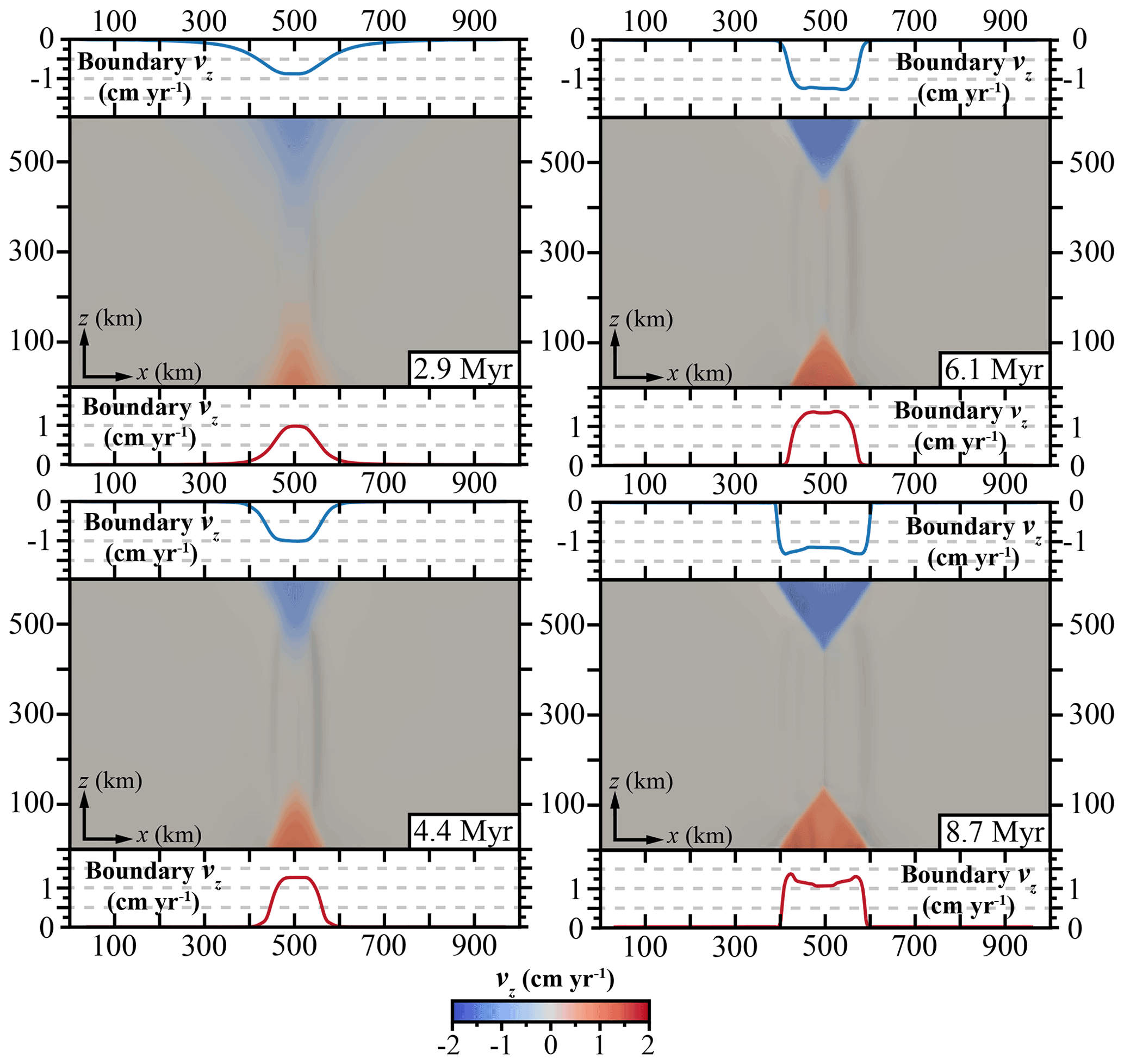
Figure 13 Map view of the z component of the velocity (v_z). Red curves represent the z component of the velocity along the boundary z_max at the surface. Blue curves represent the z component of the velocity along the boundary z_min at the surface.

4 Discussion

4.1 Alternative PDE-based approaches

Recall that the starting point of defining the PPE was purely algebraic, with the sole intention of removing the non-uniqueness associated with Eq. (5). Here we discuss two alternative PDE-based approaches constructed with a similar rationale.

Rather than enforcing Eq. (15) only along the boundary, suppose we wished to enforce it everywhere throughout the domain,

$$\begin{array}{}\text{(41)}& \mathrm{\nabla }P\cdot \widehat{\mathit{g}}=\mathit{\rho }g,\text{for}\mathit{x}\in \mathrm{\Omega }.\end{array}$$

This constraint can be interpreted as the steady-state solution of the following scalar hyperbolic PDE:

$$\begin{array}{}\text{(42)}& {\displaystyle \frac{\partial P}{\partial \mathit{\tau }}}+\widehat{\mathit{g}}\cdot \mathrm{\nabla }P=\mathit{\rho }g,\end{array}$$

where τ plays the role of a time-like parameter having units of length and $\widehat{\mathit{g}}$ plays the role of a velocity-like quantity. Along the “inflow segments” ${\mathrm{\Gamma }}_{\mathrm{in}}=\mathit{\{}\mathit{x}\in \partial \mathrm{\Omega }:\widehat{\mathit{g}}\cdot \widehat{\mathit{n}}<\mathrm{0}\mathit{\}}$ we will impose P=0¹. On the outflow segments Γ_out = ∂Ω \ Γ_in; due to the hyperbolic nature of the PDE, no boundary constraint are required. Since we seek the steady-state solution of Eq. (42), no initial condition is required, but for completeness we chose $P(\mathit{\tau }=\mathrm{0})=\mathrm{0}$. Hence, the solution of Eq. (42) is equivalent to solving

$$\begin{array}{}\text{(43)}& {\displaystyle \frac{\mathrm{d}P}{\mathrm{d}\mathit{\tau }}}=\mathit{\rho }g,\end{array}$$

along the family of characteristics given by

$$\begin{array}{}\text{(44)}& {\displaystyle \frac{\mathrm{d}\mathit{x}}{\mathrm{d}\mathit{\tau }}}=\widehat{\mathit{g}},\end{array}$$

with $P(\mathit{\tau }=\mathrm{0})=\mathrm{0}$ and $\mathit{x}(\mathit{\tau }=\mathrm{0})\in {\mathrm{\Gamma }}_{\mathrm{in}}$.

Compared to the PPE, the hyperbolic formulation has several disadvantages.

1. We have less freedom to specify how ∇P varies along the boundary. The choice of boundary conditions (BCs) is largely dictated by the “inflow” and “outflow” segments. Along outflow segments, the only constraint available is Eq. (41) evaluated on ∂Ω. If inflow occurs on any part of ∂Ω not contained in ∂Ω_surf, we have to choose a flux BC, as using P=0 does not make physical sense. Consistency may require the use of a constraint that is independent of the PDE, e.g. Eq. (16).

2. The formulation may place restrictions on the shape of ∂Ω. If we wish to avoid the definition of new flux BCs (described above), the domain must be defined such that for every ${\mathit{x}}_b\in \partial \mathrm{\Omega }\backslash \partial {\mathrm{\Omega }}_{\mathrm{surf}}$ there exists a characteristic that intersects both x_b and ∂Ω_surf.

3. The lack of flexibility in controlling the boundary behaviour of ∇P will in general result in solutions of Eq. (42) being identical to a family of 1D solutions to Eq. (2) applied in directions parallel to the direction of gravity; see Fig. 14b, d.

4. The spatial discretization required for the accurate solution of Eq. (42) is arguably more complicated to implement (on unstructured meshes) compared with discretizations for the Poisson equation. Scalable multi-level solvers for the steady-state hyperbolic problem are much more challenging to develop in comparison to the Poisson problem.

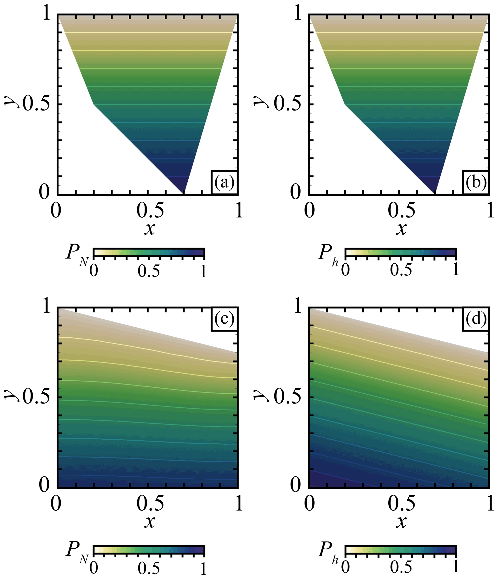
Figure 14 Pressure in non-dimensional models with constant density ρ=1. Pressure computed for a hydrostatic case in an irregularly shaped domain using (a) the normal equations (Eq. 45) and (b) the hyperbolic equation (Eq. 42). Pressure computed for a non-hydrostatic case due to topography using (c) the normal equation (Eq. 45) and (d) the hyperbolic equation (Eq. 42). The contour lines show contours of iso-pressure values every 0.1.

From a linear algebra perspective, the non-uniqueness of Eq. (5) can alternatively be addressed by (i) discretizing Eq. (5) in space, yielding Gp=F, and then (ii) solving the normal equations

$$\begin{array}{}\text{(45)}& {\mathbf{G}}^{\mathrm{T}}\mathbf{G}\stackrel{\mathrm{̃}}{\mathbf{p}}={\mathbf{G}}^{\mathrm{T}}\mathbf{F}.\end{array}$$

This approach obtains a unique solution that minimizes the following objective function:

$$\Vert \mathbf{G}\stackrel{\mathrm{̃}}{\mathbf{p}}-\mathbf{F}{\Vert }_{\mathrm{2}}.$$

In some senses, this approach is like the discrete counterpart of the PPE, in so much as G^TG are the discrete Laplacian defined on the approximation space used to represent pressure. The similarity between the pressure solution from the PPE and $\stackrel{\mathrm{̃}}{\mathbf{p}}$ are shown in Fig. 14a, c. Similar to the hyperbolic formulation, obtaining the pressure via the normal equations is restrictive from a modelling perspective as the formulation does not allow for control of the behaviour of ∇P on the boundary, and as such only the Dirichlet data on ∂Ω_surf can be specified. In Fig. 14a, c we provide snapshots of the pressure obtained from solving Eq. (45) in two different domains. Interestingly, the solutions indicate that $\mathrm{\nabla }P\cdot \widehat{\mathit{g}}$ appears to be approximately zero along the boundary despite the lack of a constraint enforcing this.

4.2 Flexibility of the PPE with respect to boundary conditions

Since the PPE is a second-order PDE, the formulation permits a range of possible boundary constraints on ∇P to be imposed. Specific choices allow one to define whether (i) the equivalent of 1D pressure profiles as would be obtained by applying Eq. (2) along a boundary face or (ii) an approximation of the pressure field on the boundary would be obtained if a complete flow field was computed in a much larger global domain.

Experiments showed that the PPE approach better approximates the total pressure computed from the momentum equation. Therefore, its use as a boundary condition (or as an initial guess) for the pressure field to solve the momentum equation is preferred over hydrostatic solutions associated with Eq. (2). Moreover, as the domain size increases, the PPE formulation gives a more accurate approximation of the total pressure than the 1D depth-integrated approach.

4.3 Implications for lithosphere deformation

In the geodynamic rift model, using the pressure computed with Eq. (7) as a boundary condition produces a velocity field perpendicular to the extension direction in the rift axis (Fig. 13). This velocity field introduces non-cylindrical deformation accommodated for by oblique and strike-slip structures (Fig. 11). The results of this study are very similar to previous studies directly applying an inflow perpendicular to the extension direction (Le Pourhiet et al., 2018; Jourdon et al., 2020). At the tip of the rift, a triangular region delimited by strike-slip faults or very oblique rift develops to accommodate the oblique velocity field. The similarity of these results shows that using open boundary conditions instead of kinematic boundary conditions in 3D may reveal first-order implications for the lithosphere strain localization. In the case of geodynamic systems presenting the characteristics of a propagating rift (or ridge) with oblique and strike-slip deformation at its tip, considering the forces applied by the surrounding material weight could be the first-order process at the origin of non-cylindrical deformation.

4.4 Linear and non-linear density

Two approaches can be considered to compute the pressure using Eq. (7). The first approach (also the simplest) is to consider that the density ρ is defined as a reference density ρ₀ that only depends on rock type for a reference state, e.g. T₀ and P₀. In that case, Eq. (7) is linear and only depends on the reference density structure. The second approach is to consider that the density ρ can vary with respect to other parameters. In our geodynamic example, we considered that the density can vary with pressure and temperature according to Eq. (38). In that case the Eq. (7) becomes non-linear. This kind of non-linearity is not rare in geodynamics, and the formulation of Eq. (38) may appear in the pressure computation when solving for an incompressible Boussinesq approximation or a compressible Stokes problem (e.g. Dannberg and Heister, 2016; King et al., 2010; Tackley, 2008).

5 Conclusions

In this study we presented a method to compute a reference pressure associated with the density structure of a domain in which we cast the problem in terms of a partial differential equation (PDE). From a practical standpoint, the PDE approach is generic (it is applicable to all spatial discretization and on any type of computational grid), efficient, and applicable in parallel computing environments. From the modelling perspective, the PDE approach has specific advantages, for example in models with a variable density structure (stationary or time-dependent) and models that employ a reference pressure as a boundary condition of the flow problem (stationary or time-dependent problems). Re-evaluating that pressure in time-dependent problems is not problematic (even if the mesh deforms) since solving the Poisson problem can be performed using optimal preconditioners (e.g. geometric or algebraic multigrid preconditioners). Importantly, the time to solve the pressure Poisson problem is a small fraction of the time required to solve the linear (or non-linear) incompressible viscous flow problem. Moreover, we also demonstrate that the PDE formulation results in a better approximation of the total pressure than the 1D depth-integrated approach in non-hydrostatic cases.

Lastly, we showed in the context of 3D geodynamic models of continental rifting that using a reference pressure as a boundary condition within the flow problem resulted in non-cylindrical velocity fields. These 3D velocity fields produced strain localization in the lithosphere along large-scale strike-slip shear zones and the formation and evolution of triple junctions.