An efficient probabilistic workflow for estimating induced earthquake parameters in 3D heterogeneous media

We present an efficient probabilistic workflow for the estimation of source parameters of induced seismic events in three-dimensional heterogeneous media. Our workflow exploits a linearized variant of the Hamiltonian Monte Carlo (HMC) algorithm. Compared to traditional Markov chain Monte Carlo (MCMC) algorithms, HMC is highly efficient in sampling high-dimensional model spaces. Through a linearization of the forward problem around the prior mean (i.e., the “best” initial model), this efficiency can be further improved. We show, however, that this linearization leads to a performance in which the output of an HMC chain strongly depends on the quality of the prior, in particular because not all (induced) earthquake model parameters have a linear relationship with the recordings observed at the surface. To mitigate the importance of an accurate prior, we integrate the linearized HMC scheme into a workflow that (i) allows for a weak prior through linearization around various (initial) centroid locations, (ii) is able to converge to the mode containing the model with the (global) minimum misfit by means of an iterative HMC approach, and (iii) uses variance reduction as a criterion to include the output of individual Markov chains in the estimation of the posterior probability. Using a three-dimensional heterogeneous subsurface model of the Groningen gas field, we simulate an induced earthquake to test our workflow. We then demonstrate the virtue of our workflow by estimating the event's centroid (three parameters), moment tensor (six parameters), and the earthquake's origin time. Using the synthetic case, we find that our proposed workflow is able to recover the posterior probability of these source parameters rather well, even when the prior model information is inaccurate, imprecise, or both inaccurate and imprecise.

1 Introduction

The need to understand earthquake source mechanisms is an essential aspect in fields as diverse as global seismology (Ekström et al., 2005), oil and gas exploration (Gu et al., 2018), hazard mitigation (Pinar et al., 2003), and space exploration (Brinkman et al., 2020). In its simplest form, an earthquake source can be described, from a physics point of view, by means of a moment tensor (MT) (Aki and Richards, 2002). An MT captures displacement, (potential) fault orientation, and the energy released during an earthquake. In a regional seismology context, MT inversions can provide insight into seismic afterslip patterns of megathrust earthquakes (e.g., Agurto et al., 2012). In the case that seismic activity is induced by anthropogenic subsurface operations, characterizing seismic sources may also prove essential (e.g., Sen et al., 2013; Langenbruch et al., 2018). With regard to oil and gas exploration, earthquake source mechanisms are often monitored when hydrocarbons are extracted or when fluids are injected into the subsurface (e.g., for fracking). In fact, such monitoring can be used to assess and mitigate the risk of ongoing injection processes activating existing faults (Clarke et al., 2019).

For the purpose of monitoring induced seismicity, arrays of seismometers can be installed over the exploration area. The waveforms recorded by these seismometers can subsequently be exploited to characterize the induced events. For example, the time of the first arrival (typically the direct P wave) is sensitive to the earthquake hypocenter and origin time. There are many inversion algorithms that exploit first arrivals to obtain estimates of earthquake hypocenters and origin times, such as the double-difference (Waldhauser and Ellsworth, 2000) and equal differential time (EDT) (Lomax, 2005) algorithms. However, to estimate MTs, it is insufficient to use only (first-arrival) travel times. In this study we therefore develop a workflow that utilizes full waveforms as input. Importantly, we pair the workflow with a probabilistic inversion algorithm.

In terms of computational efficiency, each combination of a specific inversion algorithm and a specific subsurface model has both advantages and disadvantages. In general, the main advantage of using a probabilistic approach is that the output does not consist of a single set of (source) model parameters that minimizes an objective function, but the posterior distribution (see, e.g.,  Tarantola, 2006) of the desired earthquake parameters. Probabilistic approaches, however, are significantly more computationally expensive than deterministic ones. One way to reduce the computational expense is using 1D subsurface models instead of 3D velocity models to model seismograms. Unfortunately, this can adversely affect the reliability of the obtained posterior because some of the heterogeneity of the subsurface is not accounted for (Hingee et al., 2011; Hejrani et al., 2017). In our workflow, we therefore deploy a computationally efficient probabilistic algorithm to invert for centroid (three coordinate components), origin time, and MT (six independent MT components) while at the same time utilizing a detailed 3D subsurface model.

The algorithm used in our workflow is the Hamiltonian Monte Carlo (HMC) algorithm, which, for sampling high-dimensional posterior distributions, has been shown to be significantly more efficient than the conventional probabilistic Metropolis–Hastings family of algorithms (Betancourt, 2017). Using frequencies lower than 0.1 Hz and available prior information, Fichtner and Simutė (2018) developed a variant of the HMC and demonstrated its efficiency to invert for the source parameters of a tectonic earthquake. More recently, Simute et al. (2022) demonstrated the variant's ability to estimate earthquake parameters of tectonic earthquakes while employing 3D subsurface models of the Japanese islands. In contrast to tectonic earthquakes, for which prior information regarding the event's MT, centroid, and origin time is often available, such prior information is usually absent for induced earthquakes. An insufficiently constrained prior reduces the ability and efficiency of sampling algorithms to properly sample the posterior distribution and increases the chance of the sampler getting trapped in local minima (Sen and Stoffa, 2013). In addition, compared to tectonic events, the frequency content of induced earthquake waveforms is usually significantly higher. This is because tectonic events usually occur at greater depths than induced events, and hence the higher frequencies have been attenuated more. Also, most of the studied induced events are of lower magnitudes than tectonic events (e.g., below M_w 3) and therefore do not excite frequencies below 1 Hz that effectively.

Due to the higher frequencies present in recordings of induced events, the wavelengths are significantly shorter. Layers of sediment–basin infill close to the Earth's surface may exacerbate this, since velocities usually decrease rapidly in this case. Shorter wavelengths matter because, other things being equal, they increase nonlinearity. In essence, however, the degree to which the relation between the source parameters and the recorded waveforms is nonlinear depends on the ratio between the nominal event–receiver separation and the wavelength. For example, consider (i) an induced seismic event at 3 km depth, an average P-wave velocity of 2.5 km s⁻¹, periods that range between 1 and 0.33 s, and event–receiver distances of 4 to 11 km (this study), as well as (ii) a tectonic event at 50 km depth, an average P-wave velocity of 5 km s⁻¹, periods between 100 and 15 s, and event–receiver distances of 200 to 1100 km (e.g., Fichtner and Simutė, 2018). These values correspond to ratios between event–receiver separation and wavelength that vary (approximately) between 2 and 14 (this study) and between 1 and 14 (Fichtner and Simutė, 2018). As soon as shear waves are used to perform centroid–moment tensor inversions, however, the nonlinearity in the induced seismic setting considered in this study increases relative to the tectonic case considered. This is due to the fact that $V_{\mathrm{p}}/V_{\mathrm{s}}$ ratios are typically significantly higher in the near surface (i.e., the top 1 to 2 km) than at greater depth. This is particularly the case in Groningen (e.g., Spetzler and Dost, 2017).

In this study, the absence of a well-constrained prior and an increase in nonlinearity receive significant attention. First, the challenge of a weaker prior is met by means of a workflow in which the initial prior is updated before running the HMC algorithm. In addition, multiple chains of the HMC variant are run sequentially, with the results of the current chain serving as priors for the next chain. This iterative HMC is meant to provide improved prior information resulting in an adequate linear approximation. We demonstrate the validity of our workflow using data from a synthetically generated induced earthquake, which was simulated using the velocity model of the Groningen subsurface. It should be understood that the proposed workflow is of interest for the characterization of induced seismic events in general. The Groningen case is merely chosen because of the quality and density at which the induced wavefields are sampled and the relatively high resolution of the available velocity model.

The Groningen gas field is one of the largest gas reservoirs in Europe. Since production began in 1963, more than 2115 billion m³ of natural gas has been produced from the field (van Thienen-Visser and Breunese, 2015). Due to this gas production, the reservoir layer has compacted over time, causing earthquakes that have in some cases caused damage to buildings in the Groningen province (Van Eck et al., 2006) and led to several protests against further gas extraction in the area (Verdoes and Boin, 2021). To investigate these earthquakes, an extensive seismometer array was installed, which is operated by the KNMI (the Royal Netherlands Meteorological Institute) on behalf of Nederlandse Aardolie Maatschappij (NAM) (Ntinalexis et al., 2019). Event recordings collected over the Groningen field have been used as input for several inversion algorithms. Spetzler and Dost (2017) used the EDT algorithm to invert for the hypocenters of many Groningen earthquakes. They inverted arrival times of 87 events and found that all earthquakes occurred within a depth interval of 2300 to 3500 m, with most of the events originating from the reservoir layer (approximately 3000 m depth). These findings are in line with the results of Smith et al. (2020), who used the envelopes of the seismic arrivals as input to their probabilistic algorithm. To invert for both hypocenter (or centroid) and MT, Willacy et al. (2018) took a different approach. Contrary to Spetzler and Dost (2017), who uses a 1D model to represent Groningen's subsurface, they utilized a 3D heterogeneous model similar to Smith et al. (2020) and used the model to generate synthetic waveforms to perform a full-waveform deterministic MT inversion. The results of Willacy et al. (2018), however, only focused on pure double-couple sources, which might not capture the true source dynamics. In fact, Dost et al. (2020) recently followed a probabilistic approach to invert event centroids and MTs of a selected number of events and consistently found the (non-double-couple) isotropic component of the MT to be dominant and negative. The latter is in agreement with expectations for a compacting medium. Similar to Willacy et al. (2018), they invert waveforms but employ 1D local subsurface models to generate the modeled seismograms.

In what follows, we first introduce the forward problem of obtaining surface displacements (recorded wavefields) due to induced seismic source activity, including the description of a seismic source in terms of elementary moment tensors. Subsequently, we introduce the Bayesian formulation and detail the linearized HMC algorithm. Afterward, we proceed with the description and implementation of our workflow, which involves several steps that are specific to the characterization of induced seismic sources. We then test the proposed workflow using synthetic recordings of an induced earthquake source. We end by giving a perspective discussion of our results, including an outlook of applying our workflow to actual field recordings of induced earthquakes from the Groningen gas field.

2 Forward problem

As with all Markov chain Monte Carlo algorithms, HMC involves an evaluation of forward-modeled data against observed data. In our case, this evaluation is between (forward) modeled surface displacement and observed displacement. Specifically, we compute synthetic displacement seismograms u due to a moment tensor source M (Aki and Richards, 2002) as

$$\begin{array}{}\text{(1)}& u_i(x_{\mathrm{r}},t)=\sum _{j,k}{M}_{jk}(x_{\mathrm{a}},t)*G_{ij,k}{x}_{\mathrm{r}};x_{\mathrm{a}},t),\end{array}$$

with x_r the location at which u is recorded, x_a the source location, and * representing temporal convolution. Subscripts i,j, and k take on values of 1, 2, and 3 such that a vector can be decomposed in three Cartesian components, associated with the x₁, x₂, and x₃ axis, respectively. G is the Green's function, and its first subscript represents its recorded component. The second subscript indicates the direction in which an impulsive (delta function) force is acting. The comma after the second subscript represents a spatial derivative, and the subscript after the comma indicates the direction in which the derivative is taken. Each component of M represents the strength of force couples. Together, the nine constants M_jk constitute the second-order seismic moment tensor M. The MT effectively approximates a seismic source by collapsing it into a single point. Furthermore, due to conservation of angular momentum, The MT has only six independent components (e.g., Aki and Richards, 2002; Jost and Herrmann, 1989).

Instead of repeatedly computing u for each source–receiver pair location, it is convenient to exploit source–receiver reciprocity. That is, we exploit the fact that $G_{ij}\left(x_{\mathrm{r}};x_{\mathrm{a}},t\right)=G_{ji}\left(x_{\mathrm{a}};x_{\mathrm{r}},t\right)$ (Aki and Richards, 2002; Wapenaar and Fokkema, 2006), which yields

$$\begin{array}{}\text{(2)}& u_i(x_{\mathrm{r}},t)=\sum _{j,k}{M}_{jk}(x_{\mathrm{a}},t)*G_{ji,k}(x_{\mathrm{a}};x_{\mathrm{r}},t).\end{array}$$

To facilitate the computation of seismograms for a specific M, we follow the work of Mustać and Tkalčić (2016), who use six independent tensors that they call elementary moment tensors as decomposed by Kikuchi and Kanamori (1991):

$$\begin{array}{}\text{(3)}& \begin{array}{ll}{\mathbf{M}}^{\mathrm{1}}=\left(\begin{array}{ccc}\mathrm{0}& \mathrm{1}& \mathrm{0}\\ \mathrm{1}& \mathrm{0}& \mathrm{0}\\ \mathrm{0}& \mathrm{0}& \mathrm{0}\end{array}\right)& {\mathbf{M}}^{\mathrm{2}}=\left(\begin{array}{ccc}\mathrm{0}& \mathrm{0}& \mathrm{1}\\ \mathrm{0}& \mathrm{0}& \mathrm{0}\\ \mathrm{1}& \mathrm{0}& \mathrm{0}\end{array}\right)\\ {\mathbf{M}}^{\mathrm{3}}=\left(\begin{array}{ccc}\mathrm{0}& \mathrm{0}& \mathrm{0}\\ \mathrm{0}& \mathrm{0}& -\mathrm{1}\\ \mathrm{0}& -\mathrm{1}& \mathrm{0}\end{array}\right)& {\mathbf{M}}^{\mathrm{4}}=\left(\begin{array}{ccc}-\mathrm{1}& \mathrm{0}& \mathrm{0}\\ \mathrm{0}& \mathrm{0}& \mathrm{0}\\ \mathrm{0}& \mathrm{0}& \mathrm{1}\end{array}\right)\\ {\mathbf{M}}^{\mathrm{5}}=\left(\begin{array}{ccc}\mathrm{0}& \mathrm{0}& \mathrm{0}\\ \mathrm{0}& -\mathrm{1}& \mathrm{0}\\ \mathrm{0}& \mathrm{0}& \mathrm{1}\end{array}\right)& {\mathbf{M}}^{\mathrm{6}}=\left(\begin{array}{ccc}\mathrm{1}& \mathrm{0}& \mathrm{0}\\ \mathrm{0}& \mathrm{1}& \mathrm{0}\\ \mathrm{0}& \mathrm{0}& \mathrm{1}\end{array}\right)\end{array}.\end{array}$$

Under the assumption that each of these elementary moment tensors has the same time dependence (e.g., in the case of pure shear, this would imply that faulting occurs along a straight “trajectory”), a specific M can be described as a linear combination of these elementary moment tensors, i.e.,

$$\begin{array}{}\text{(4)}& \begin{array}{rl}\mathbf{M}& =\sum _{n=\mathrm{1}}^{\mathrm{6}}{a}_n{\mathbf{M}}^n\\ & =\left(\begin{array}{ccc}-a_{\mathrm{4}}+a_{\mathrm{6}}& a_{\mathrm{1}}& a_{\mathrm{2}}\\ a_{\mathrm{1}}& -a_{\mathrm{5}}+a_{\mathrm{6}}& -a_{\mathrm{3}}\\ a_{\mathrm{2}}& -a_{\mathrm{3}}& a_{\mathrm{4}}+a_{\mathrm{5}}+a_{\mathrm{6}}\end{array}\right),\end{array}\end{array}$$

where the coefficients a_n ($n=\mathrm{1},\mathrm{2},\mathrm{\dots },\mathrm{6}$) are usually referred to as expansion coefficients. In this study, we assume instantaneous rupturing of the source. This is not an uncommon assumption for (relatively small) induced seismic events. This assumption implies that the time dependence of an MT is modeled using a Heaviside function. Using the decomposition above and source–receiver reciprocity, we compute elementary seismograms $S_i^n$ as

$$\begin{array}{}\text{(5)}& S_i^n(x_{\mathrm{r}};x_{\mathrm{a}},t)=\sum _{j,k}{G}_{ji,k}(x_{\mathrm{a}};x_{\mathrm{r}},t)*M_{jk}^n\left(t\right).\end{array}$$

Consequently, we obtain

$$\begin{array}{}\text{(6)}& u_i\left(x_{\mathrm{r}};x_{\mathrm{a}},t\right)=\sum _{n=\mathrm{1}}^{\mathrm{6}}{a}_n{S}_i^n(x_{\mathrm{r}};x_{\mathrm{a}},t).\end{array}$$

In practice, all $S_i^n(x_{\mathrm{r}};x_{\mathrm{a}},t)$ are computed for a finite number of x_a on a predetermined subsurface grid with a specific grid spacing. We detail the numerical implementation of computing the $S_i^n(x_{\mathrm{r}};x_{\mathrm{a}},t)$ further below.

3 Hamiltonian Monte Carlo

The HMC algorithm originated from the field of classical mechanics and its application to statistical mechanics (Betancourt, 2017). It is known to be one of the most efficient probabilistic algorithms within the Markov chain Monte Carlo (MCMC) family. For our workflow, we apply a variant of the HMC algorithm that utilizes a linearization of the forward problem. Therefore, we include several initial steps in our workflow to obtain priors that enable meaningful linearization. In total, our workflow estimates 10 source parameters. These are the centroid x_a (three components), the origin time T0, and the MT (six independent MT components).

Similar to other probabilistic algorithms, HMC is deployed in the context of Bayesian inference. The objective of Bayesian inference is to obtain an estimate of the posterior probability distribution ρ(m|d) that approaches the true posterior probability distribution (from here on, we will refer to ρ(m|d) as being “the posterior”). This approach combines the likelihood ρ(d|m) of the observed data given the modeled data with the simultaneous assimilation of the distribution of prior knowledge ρ(m), i.e.,

$$\begin{array}{}\text{(7)}& \mathit{\rho }\left(\mathit{m}\right|\mathit{d})\propto \mathit{\rho }(\mathit{d}\left|\mathit{m}\right)\mathit{\rho }\left(\mathit{m}\right),\end{array}$$

where m that contains model parameters and d a vector containing the observed data. The likelihood evaluates a model m against the observed data d by evaluating the misfit between the latter and forward-modeled data associated with m.

The HMC algorithm relies on the sequential calculation of two quantities. These are the potential energy U, which explicitly quantifies ρ(m|d), and the kinetic energy K, which is a function of momentum vector p. Together, they make up the Hamiltonian H(m,p), which represents the total energy of a system (Neal, 2011) and is written as follows:

$$\begin{array}{}\text{(8)}& \begin{array}{rl}H=K\left(\mathit{p}\right)+U\left(\mathit{m}\right),& \text{with}U\left(\mathit{m}\right)=-\ln \mathit{\rho }(\mathit{m}\mid \mathit{d})\\ & \text{and}K\left(\mathit{p}\right)={\mathit{p}}^T{\mathbf{R}}^{-\mathrm{1}}\mathit{p}/\mathrm{2}.\end{array}\end{array}$$

A model m can be interpreted as the position of a particle within phase space. The phase space has a dimension that is twice the dimension of the model space (i.e., this dimension coincides with the length of the vector m multiplied by 2). By having the same dimension as m, the elements of the auxiliary momentum vector p are therefore needed to complement each dimension of the model space (Betancourt, 2017). The movement of the particle is highly dependent on the mass matrix R, which therefore often acts as a tuning parameter (Fichtner et al., 2019, 2021). The mass matrix affects the “distance” a particle travels and ideally coincides with the posterior covariance matrix. Given a certain momentum p, the particle is allowed to travel for a certain (artificial) time τ while in conjunction fulfilling Hamilton's equations:

$$\begin{array}{}\text{(9)}& {\displaystyle \frac{d\mathit{m}}{d\mathit{\tau }}}={\displaystyle \frac{\partial K}{\partial \mathit{p}}},{\displaystyle \frac{d\mathit{p}}{d\mathit{\tau }}}=-{\displaystyle \frac{\partial U}{\partial \mathit{m}}}.\end{array}$$

We parenthetically coined τ an artificial time because it should not be confused with physical time t. It is this artificial time with which the model moves through phase space: at time τ, the particle arrives at a new location representing a new model m(τ). The new model and momentum vectors are associated with updated potential and kinetic energies, respectively, and hence a higher or lower Hamiltonian H(p(τ),m(τ)). Given the probability θ that the particle will stay at the new location, the acceptance probability is given by

$$\begin{array}{}\text{(10)}& \mathit{\theta }=min\left[\mathrm{1},{\displaystyle \frac{\exp [-H(\mathit{p}\left(\mathit{\tau }\right),\mathit{m}\left(\mathit{\tau }\right)\left)\right]}{\exp [-H(\mathit{p},\mathit{m}\left)\right]}}\right].\end{array}$$

By sequentially evaluating Eqs. (8) to (10) in an iterative manner, we collect all locations (models) visited by the particle, except for a number of initial models (representing the burn-in period). The density of the collected models asymptotically approaches the posterior probability distribution.

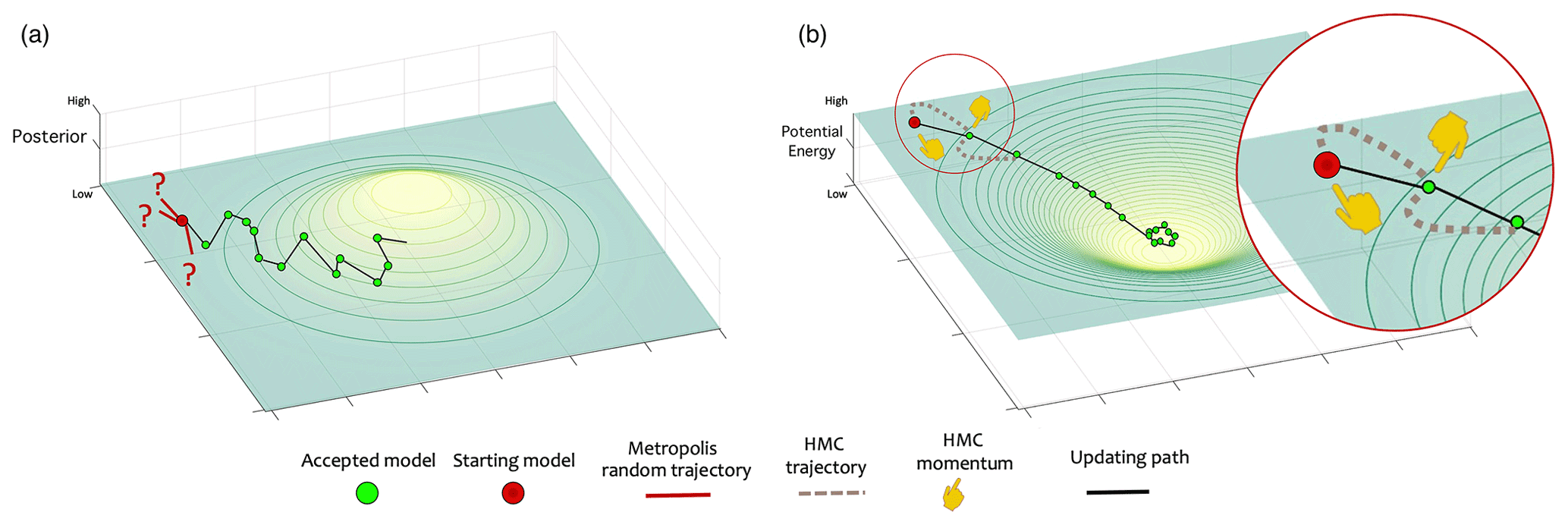
Figure 1 Comparison between the sampling strategy of the (a) Metropolis algorithm and (b) Hamiltonian Monte Carlo algorithm.

In Fig. 1, we visualize the sampling behavior of both the Metropolis algorithm (Fig. 1a) and the HMC algorithm (Fig. 1b) for a 2D joint probability distribution. Note that the Metropolis algorithm is a special case of the Metropolis–Hastings algorithm in the sense that the proposal distribution is symmetric (Hoff, 2009). Both algorithms start with the same starting model, which is represented by the red ball. The low a posteriori probability of this initial model corresponds to a high U. The question marks in Fig. 1a represent randomly selected models by the Metropolis algorithm, which were not accepted due to their relatively low acceptance probability. Hence, each of these question marks involves a (computationally expensive) solution to the forward problem. Instead of using random sampling, in the HMC algorithm, the particle within phase space moves along trajectories obtained by solving Eq. (9), leading to the particle being exerted towards areas with low U, as illustrated in Fig. 1b. Furthermore, in Fig. 1b, the result of solving Eq. (9) (i.e., the HMC trajectory) is represented by the brown dashed lines, and the pointing finger represents the momentum vector p. For both the HMC and Metropolis algorithms, an accepted model serves as a starting model for the next sample. Although probabilistic in terms of acceptance probabilities, the trajectories of the HMC algorithm are deterministically guided by $\partial U/\partial \mathit{m}$ as shown in Eq. (9). Therefore, the algorithm is also known as the hybrid Monte Carlo algorithm (Duane et al., 1987). Thus, after proper tuning, the HMC algorithm requires less sampling than the Metropolis algorithm to converge, which makes the HMC algorithm computationally more efficient.

Assuming Gaussian-distributed, uncorrelated, and coinciding data variance ${\mathit{\sigma }}_{\mathrm{d}}^{\mathrm{2}}$, we can write U as (Fichtner and Simutė, 2018)

$$\begin{array}{}\text{(11)}& \begin{array}{rl}U\left(\mathit{m}\right)=& {\displaystyle \frac{\mathrm{1}}{\mathrm{2}T}}\sum _{r=\mathrm{1}}^{N_{\mathrm{r}}}\sum _{i=\mathrm{1}}^{\mathrm{3}}\underset{\mathrm{0}}{\overset{T}{\int }}{\mathit{\sigma }}_{\mathrm{d}}^{-\mathrm{2}}\\ & \times {\left[u_i(x_{\mathrm{r}},t;\mathit{m})-u_i^{\text{obs}}(x_{\mathrm{r}},t)\right]}^{\mathrm{2}}\mathrm{d}t\\ & +{\displaystyle \frac{\mathrm{1}}{\mathrm{2}{N}_{\mathrm{m}}}}(\mathit{m}-{\mathit{m}}^{\mathrm{0}}{)}^{\mathit{⊺}}{\mathbf{C}}_{\mathrm{m}}^{-\mathrm{1}}(\mathit{m}-{\mathit{m}}^{\mathrm{0}}).\end{array}\end{array}$$

In our context, x_r represents the locations of the N_r three-component KNMI seismometers ($r=\mathrm{1},\mathrm{2},\mathrm{3},\mathrm{\dots },N_{\mathrm{r}}$). Furthermore, T is the length of observed and forward modeled seismograms in time, N_m the number of model parameters (10 in our case), m⁰ a vector containing prior means, and C_m the prior covariance matrix. In application to field data, $u_i^{\text{obs}}$ would represent field recordings by seismometers, but in this study we restrict ourselves to a numerically simulated induced event.

4 Linearization of the forward problem

In our workflow, most of the computational burden in running HMC involves the evaluation of Eq. (9). This is because for each dτ we have to evaluate $\partial U/\partial \mathit{m}$. To speed up the process, we use a variant of the HMC algorithm introduced by Fichtner and Simutė (2018), in which $\mathbf{u}(x_{\mathrm{r}},t;\mathit{m})$ is approximated by means of an expansion around the prior mean, i.e., around m⁰:

$$\begin{array}{}\text{(12)}& \begin{array}{rl}{u}_i(x_{\mathrm{r}},t;\mathit{m})=& u_i\left(x_{\mathrm{r}},t;{\mathit{m}}^{\mathrm{0}}\right)\\ & +\sum _{p=\mathrm{1}}^{N_{\mathrm{m}}}{\displaystyle \frac{\partial }{\partial m_p}}{u}_i\left(x_{\mathrm{r}},t;{\mathit{m}}^{\mathrm{0}}\right)\left(m_p-m_p^{\mathrm{0}}\right).\end{array}\end{array}$$

Substituting this linearized expression in Eq. (11) gives

$$\begin{array}{}\text{(13)}& \begin{array}{rl}U\left(\mathit{m}\right)=& {\displaystyle \frac{\mathrm{1}}{\mathrm{2}}}\sum _{p,q=\mathrm{1}}^{N_{\mathrm{m}}}\left(m_p-m_p^{\mathrm{0}}\right)A_{pq}\left(m_q-m_q^{\mathrm{0}}\right)\\ & +\sum _{p=\mathrm{1}}^{N_{\mathrm{m}}}{b}_p\left(m_p-m_p^{\mathrm{0}}\right)+{\displaystyle \frac{\mathrm{1}}{\mathrm{2}}}c,\end{array}\end{array}$$

where A_pq, b_p, and c read

$$\begin{array}{}\text{(14)}& {\displaystyle }\begin{array}{rl}{A}_{pq}=& {\displaystyle \frac{\mathrm{1}}{T{\mathit{\sigma }}_{\mathrm{d}}^{\mathrm{2}}}}\sum _{r=\mathrm{1}}^{N_{\mathrm{r}}}\sum _{i=\mathrm{1}}^{\mathrm{3}}\underset{\mathrm{0}}{\overset{T}{\int }}[{\displaystyle \frac{\partial }{\partial m_p}}{u}_i\left(x_{\mathrm{r}},t;{\mathit{m}}^{\mathrm{0}}\right)\\ & \times {\displaystyle \frac{\partial }{\partial m_q}}{u}_i\left(x_{\mathrm{r}},t;{\mathit{m}}^{\mathrm{0}}\right)]\mathrm{d}t+{\displaystyle \frac{\mathrm{1}}{N_{\mathrm{m}}{\mathit{\sigma }}_{\mathrm{m}}^{\mathrm{2}}}},\end{array}\text{(15)}& {\displaystyle }\begin{array}{rl}{b}_p=& {\displaystyle \frac{\mathrm{1}}{T{\mathit{\sigma }}_{\mathrm{d}}^{\mathrm{2}}}}\sum _{r=\mathrm{1}}^{N_{\mathrm{r}}}\sum _{i=\mathrm{1}}^{\mathrm{3}}\underset{\mathrm{0}}{\overset{T}{\int }}\left[u_i\left(x_{\mathrm{r}},t;{\mathit{m}}^{\mathrm{0}}\right)-u_i^{\text{obs}}(x_{\mathrm{r}},t)\right]\\ & \times {\displaystyle \frac{\partial }{\partial m_p}}{u}_i\left(x_{\mathrm{r}},t;{\mathit{m}}^{\mathrm{0}}\right)\mathrm{d}t,\end{array}\end{array}$$

and

$$\begin{array}{}\text{(16)}& c={\displaystyle \frac{\mathrm{1}}{T{\mathit{\sigma }}_{\mathrm{d}}^{\mathrm{2}}}}\sum _{r=\mathrm{1}}^{N_{\mathrm{r}}}\sum _{i=\mathrm{1}}^{\mathrm{3}}\underset{\mathrm{0}}{\overset{T}{\int }}{\left[u_i\left(x_{\mathrm{r}},t;{\mathit{m}}^{\mathrm{0}}\right)-u_i^{\text{obs}}(x_{\mathrm{r}},t)\right]}^{\mathrm{2}}\mathrm{d}t.\end{array}$$

Differentiating Eq. (13) with respect to m_p, we have (Fichtner and Simutė, 2018)

$$\begin{array}{}\text{(17)}& {\displaystyle \frac{\partial U}{\partial m_p}}=\sum _{q=\mathrm{1}}^{N_{\mathrm{m}}}{A}_{pq}\left(m_q-m_q^{\mathrm{0}}\right)+b_p,\end{array}$$

which, together with the random momentum vector, determines the HMC trajectory.

Because the displacement depends linearly on the moment tensor components (see Eqs. 5 and 6), Eq. (12) is exact with respect to these parameters. The dependence on the other parameters is nonlinear, and this nonlinearity increases as the frequency of the input data increases. Therefore, in the case of induced events, which usually generate higher frequencies than stronger, regional events, the nonlinearity is considerably higher. Hence, to have a tolerable linearization, accurate priors are required when it comes to the centroid and origin time. Without sufficiently accurate priors, the above HMC variant will struggle to sample the mode containing the global minimum of the potential energy. Therefore, we propose an approach that involves an initial estimation of the prior mean in order to permit this linearization. This is detailed further below.

5 Numerical implementation

In practice, the elementary seismograms discussed in Sect. 2 are computed for a finite number of possible centroid locations. That is, prior to our probabilistic inversion, we generate a database of these seismograms. This database contains, for each possible source location x_a and receiver location x_r ($r=\mathrm{1},\mathrm{\dots },N_{\mathrm{r}}$), a total of 3 × 6 = 18 elementary seismograms (three components for each of the six elementary moment tensors). In our case, each x_r corresponds to a (KNMI) seismometer location that recorded the induced event. The elementary seismograms are computed using the spectral element software SPECFEM3D-Cartesian (Komatitsch and Tromp, 2002), and we exploited spatial reciprocity while doing so. We use an existing detailed Groningen velocity model (Romijn, 2017) for this purpose from which we construct a regular grid of the model using the gnam and PyAspect Python packages that are available at https://github.com/code-cullison/gnam (last access: 12 August 2022) and https://github.com/code-cullison/pyaspect (last access: 12 August 2022).

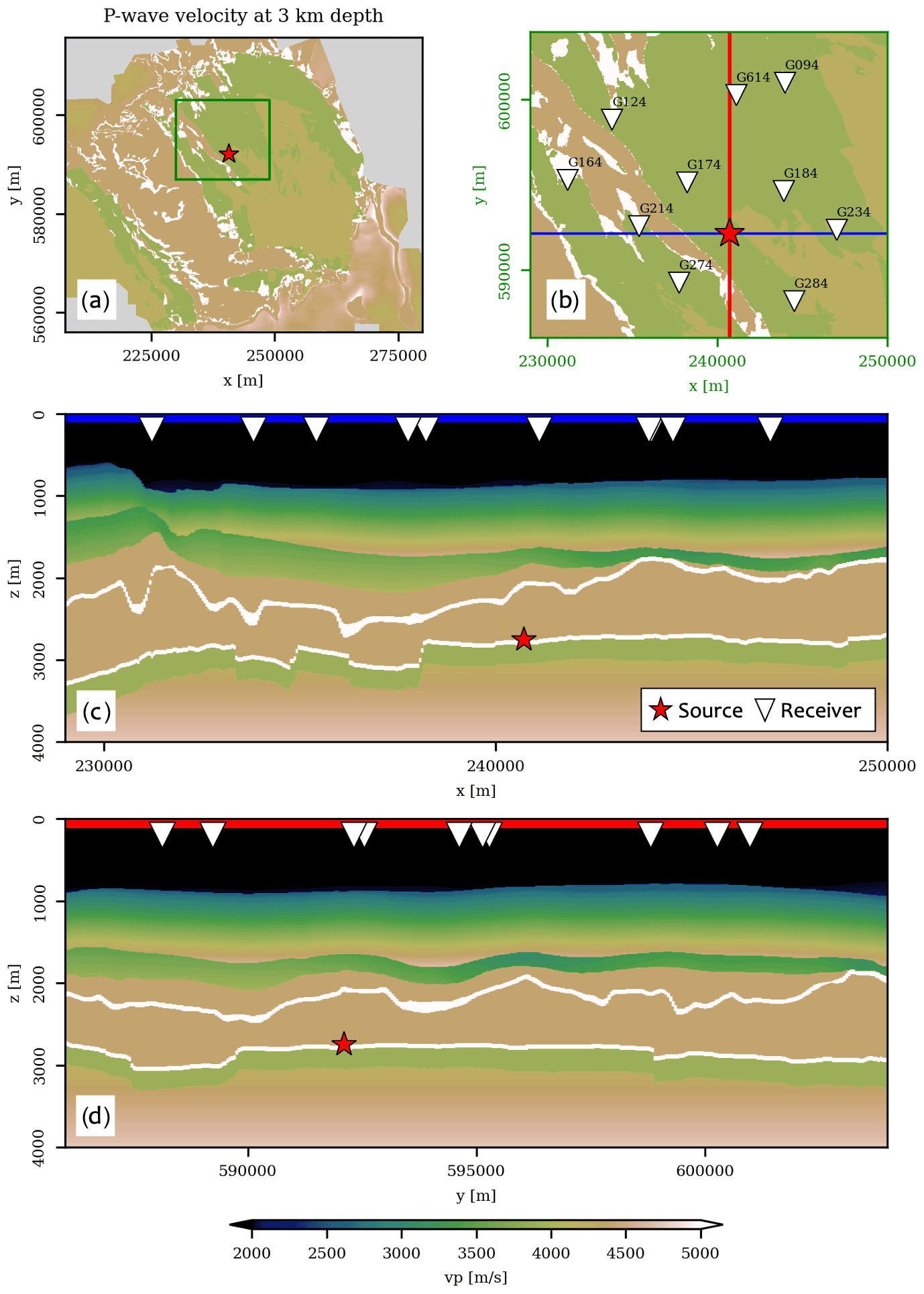
Figure 2 Scenario of an induced earthquake in the Groningen area. (a) Horizontal slice of the Groningen P-wave velocity model. (b) Zoom of the area indicated by the green rectangle in (a). Inverted triangles indicate locations of KNMI stations (i.e., the x_r). (c) Vertical slice along the blue line in (b). (d) Vertical slice along the red line in (b).

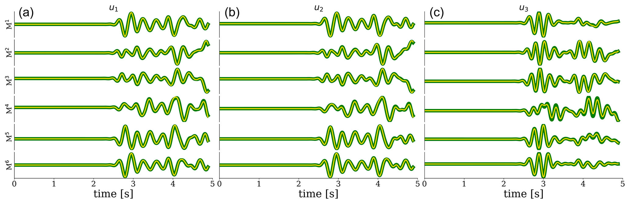
Figure 3 Comparison between elementary seismograms due to a source at the actual location (red star) and the receiver at G094 (green) as well as the elementary seismograms resulting from the implementation of source–receiver reciprocity (yellow). The equality of the traces confirms successful implementation of source–receiver reciprocity. Along the vertical axis, all six (independent) elementary seismograms are depicted. (a–c) Plots show particle displacement in the x₁, x₂, and x₃ direction, respectively.

To confirm the successful implementation of source–receiver reciprocity, we simulate a scenario of an induced event in the Groningen gas reservoir (Fig. 2). The centroid is indicated with a red star, and the receivers are depicted as white triangles. At each location, the wavefield is “recorded” at 200 m depth by the deepest of a series of four borehole geophones (Ruigrok and Dost, 2019). The elementary seismograms computed at the location of KNMI station G094 are shown in Fig. 3 (green), and superimposed on top (yellow) are the waveforms resulting from the application of source–receiver reciprocity. All seismograms are band-pass-filtered between 1 and 3 Hz, similar to the passband used by Dost et al. (2020).

We integrate the above HMC variant into our workflow by implementing a leapfrog algorithm for evaluating Eq. (9). Furthermore, we define dτ as suggested by Neal (2011) to ensure numerical stability and set a fixed value for τ for all chains. The construction of the mass matrix R is discussed in the next section.

6 An iterative approach

The performance of the linearized HMC variant strongly depends on the prior means (see Eq. 12). For that reason, we propose a workflow in which the algorithm is run iteratively, with each iteration involving an update of the priors to allow for an updated linearization. Specifically, instead of evaluating Eqs. (14)–(16) once, we run a sequence of HMC chains. For each successive chain, the posterior means and standard deviations from the previous chain act as prior means and entries for R in the new chain (i.e., the next iteration). For the first chain in the sequence, the “initial” prior means (i.e., m⁰) are obtained via a specific scheme integrated into the workflow. The estimation of these prior means is described in more detail in the subsection below.

We test our workflow for an induced event shown in Fig. 2. We set the MT components to 9 × 10¹³, −1E × 10¹³, −3 × 10¹³, 8 × 10¹³, 5 × 10¹³, and 4 × 10¹³ Nm for M₁₁, M₂₂, M₃₃, M₁₂, M₁₃, and M₂₃, respectively. Using the moment–magnitude relation given by Gutenberg (1956) and Kanamori (1977), this moment tensor can be shown to correspond to an earthquake of magnitude M_w 3.28. We also add noise to our synthetic seismograms in order to make our experiment more realistic. This noise is added in the frequency domain by multiplying the (complex) spectrum of each synthetic seismogram with a bivariate normal distribution that has a zero mean and a standard deviation of 15 % of the amplitude of the seismogram at the dominant frequency. As a result, this noise will not only give amplitude variations but also varying time shifts with respect to the true synthetic seismograms. When running the Markov chains, we assume the square root of the data variance (σ_d) to be 30 % of the maximum amplitude of each seismogram. Admittedly, this is rather arbitrary, and in the application to field data, the data uncertainty has to be estimated from the obtained seismograms themselves. Finally, we set the origin time to 14 s.

6.1 Prior mean estimation

Before running the first HMC chain, we need to estimate the initial prior means and variances. In short, we propose an approach in which a first-arrival-based algorithm is used to estimate the centroid. Subsequently, the origin time can be estimated, after which Eq. (17) can be used to compute the prior means for the individual moment tensor components. Each of these steps is now discussed in more detail.

Numerous algorithms exist that allow one to estimate an earthquake's hypocenter and/or centroid. Here we propose using first-arrival-based algorithms for this purpose since these are computationally more efficient than waveform-based algorithms. First-arrival-based algorithms only require the computation of the P- and S-wave arrival times, and by adopting a high-frequency approximation (e.g., Aki and Richards, 2002), these arrivals can be found by running one of the various eikonal solvers (e.g., Noble et al., 2014). For example, the EDT method detailed in Lomax (2005) can be used for this purpose (Masfara and Weemstra, 2021).

As an alternative to using a first-arrival-based algorithm, the prior means of the centroid can instead be retrieved from the literature if it exists. For example, in the case of the induced seismicity in the Groningen field, Smith et al. (2020) have shown that they could resolve hypocenters with maximum uncertainties of 150 and 300 m for epicenter and depth, respectively. Their results could be considered priors. Another option is to use the epicenters from the KNMI earthquake database, which by default all have depths set to 3 km.

Given a centroid prior mean that was either calculated or acquired from the literature, the prior mean of the origin time can be estimated by computing the P-wave travel times from a centroid prior to each of the receivers. These travel times can be computed using the same eikonal solver that was used to obtain the centroid prior (e.g., the fast marching method; Sethian and Popovici, 1999). By subtracting the computed travel times from the observed (picked) first-arrival times and averaging across receivers, an initial origin-time prior mean can be obtained.

To refine the initial origin-time prior estimate, we cross-correlate the envelope of the observed seismograms $\text{env}\left[u_i^{\text{obs}}\right(x_{\mathrm{r}},t\left)\right]$ with the envelope of the forward-modeled seismograms $\text{env}\left[u\right(x_{\mathrm{r}},t,{\mathit{m}}^{\mathrm{0}}\left)\right]$. We do this for each component of each receiver location individually. The forward-modeled seismograms are computed with full-waveform modeling (detailed in Sect. 5) using the initial prior means for centroid and origin time, as well as given arbitrary MT components. Specifically, we compute

$$\begin{array}{}\text{(18)}& \begin{array}{rl}{\text{T0}}_{\text{shift}}=& {\text{argmax}}_t\sum _{r=\mathrm{1}}^{N_{\mathrm{r}}}\sum _{i=\mathrm{1}}^{\mathrm{3}}\text{env}\left[u_i\left(x_{\mathrm{r}},t;{\mathit{m}}^{\mathrm{0}}\right)\right]\\ & \times \text{env}\left[u_i^{\text{obs}}(x_{\mathrm{r}},t)\right],\end{array}\end{array}$$

where T0_shift is the additional time shift that needs to be added to the initial origin-time prior mean to obtain the refined origin-time prior.

We test Eq. (18) using the synthetic earthquake shown in Fig. 2. For this test, we add 600 m to the true x₁, x₂, and x₃ centroid components, and we impose a (rather aggressive) 9 s time shift with respect to the true origin time. Note that this implies that we did not employ the aforementioned procedure to obtain initial centroid and origin-time priors because this would result in a centroid and origin-time estimate that would be too close to the true centroid and origin time – essentially rendering the use of Eq. (18) unnecessary. In other words, we deliberately impose large deviations from the true values to show the merit of using Eq. (18).

Figure 4 The results of estimating the prior mean of origin time using Eq. (18) (d), given the envelopes of modeled displacements (a), noisy synthetic “observed” seismograms (b), and the convolution between (a) and (b) in (c).

Given arbitrary MT components, we show in Fig. 4 the result of applying Eq. (18) to vertical surface displacements. In Fig. 4a, we depict the envelopes of modeled seismograms given available prior means (i.e., 600 m deviation from the true x₁, x₂, and x₃ values and 9 s from the true T0). Figure 4b shows the noisy synthetic “observed” seismograms, and Fig. 4c is the result of applying Eq. (18) to each of the displacement envelopes. In Fig. 4d, we show the result of stacking all signals in Fig. 4c. The vertical blue line indicates the time at which the stack of the cross-correlated envelopes attains its maximum value, i.e., T0_shift; the vertical red line represents the deviation of the initial origin-time prior from the true origin time (i.e., 9 s in this example).

Having sufficiently accurate prior means for the centroid and origin time, we then estimate the prior mean of the MT. For this purpose, we keep the centroid and origin time constant but solve for the remaining six parameters (the independent MT elements). In Sect. 4, we showed that because Eq. (13) is a quadratic function of m, its derivative is linear in m (see Eq. 17). This first derivative hence coincides with zero for that model for which U(m) attains its (global) minimum value. As such, setting this derivative to zero allows us to obtain a first estimate (i.e., prior means) of the moment tensor components. Setting the left-hand side of Eq. (17) to zero yields

$$\begin{array}{}\text{(19)}& \mathit{m}={\mathbf{A}}^{-\mathrm{1}}\left(\mathbf{A}{\mathit{m}}^{\mathrm{0}}-b\right)={\mathit{m}}^{\mathrm{0}}-{\mathbf{A}}^{-\mathrm{1}}b.\end{array}$$

It should be understood that Eq. (19) is implemented with T0 and centroid fixed. Hence, the model vector has only six elements, and A is a 6 by 6 matrix. The quadratic nature of U in Eq. (13) furthermore implies that arbitrary values can be chosen for the initial moment tensor components in m⁰. In fact, in the absence of noise and the correct prior means for the centroid and origin time, the MT priors estimated using Eq. (19) will coincide with the true MT components.

In practice, the prior means resulting from Eq. (19) may still deviate significantly from the true values due to the inaccuracy of the initial centroid and origin-time priors. Solving Eq. (19) nevertheless provides sufficiently accurate prior information regarding the magnitude of the induced event. Finally, it is useful to draw a parallel with typical least-squares optimization problems (e.g., Virieux and Operto, 2009). In such a context, A is analogous to the Hessian, and the difference between m and m⁰ in Eq. (19) can be considered the model update vector.

Figure 5 Full workflow of our iterative HMC scheme.

6.2 Full workflow

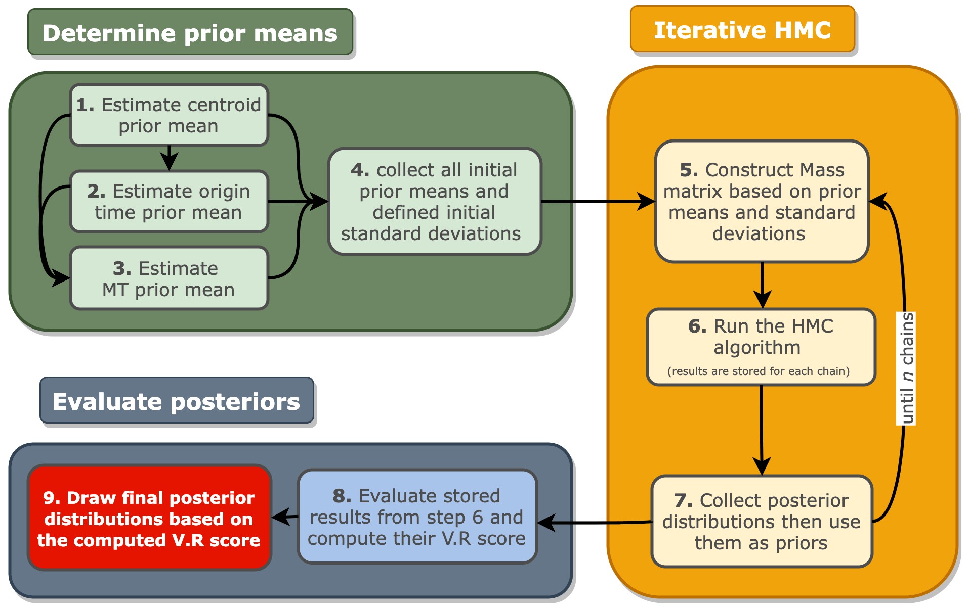
In Fig. 5, we illustrate our entire workflow. The main component of the workflow is the iterative HMC procedure, which is preceded by the (just-described) determination of the initial prior and succeeded by the evaluation of the posteriors.

The determination of the initial prior consists of the following four steps.

• 1.

  Estimate the initial prior mean for the centroid, either by running a first-arrival-based probabilistic inversion algorithm or by extracting it from existing literature.

• 2.

  Estimate the initial prior mean of the origin time using (P-wave) travel times from the centroid obtained in step 1 to the receiver locations. This estimate is refined by evaluating Eq. (18) using an arbitrary MT.

• 3.

  Estimate the initial prior mean of the MT by fixing centroid and origin time to their prior means (steps 1 and 2) and solving Eq. (19). The sought-after MT prior means are contained in m upon substitution of arbitrary MT components in m⁰.

• 4.

  Determine the standard deviation for each of the 10 model parameters: centroid (3), origin time, and moment tensor (6). These standard deviations are needed to construct our first mass matrix R. Ideally, R is the posterior covariance matrix. Here we approximate it by a 10 × 10 diagonal matrix with the following entries for the diagonal. For the first three entries (representing the centroid), we take the standard deviation of the centroid prior mean obtained in step 1. For the entry representing origin time, we use half the period of the dominant frequency in the recordings. For the MT components, we use 5 % of the minimum absolute value of the MT prior means obtained by solving Eq. (19).

Now that the (initial) prior means and standard deviations are determined, the HMC variant is run iteratively up to n chains (yellow box in Fig. 5). A test for chain convergence might be required to determine the number of chains needed, and it is highly dependent on the quality of the prior means, data uncertainty, model uncertainty, initial model, and dominant frequency of the observed recordings. In our example (detailed below), approximately 10 chains are sufficient when the distance between the initial estimation of the centroid and the true centroid is less than 700 m. The separate steps of the iterative HMC procedure are the following.

• 5.

  Collect the prior means and associated standard deviations, and construct the mass matrix R. For the first chain, the output from steps 1 to 4 is used as input. In subsequent chains, they are extracted from the posterior of the previous HMC chain. In this step, A (Eq. 14), b (Eq. 15) and c (Eq. 16) are also recomputed.

• 6.

  Run a new HMC chain with a preset number of iterations and burn-in period. Note that for each chain, the results are stored for latter use.

• 7.

  Collect the results. The means and standard deviations will serve as input of for the next iteration (see step 5).

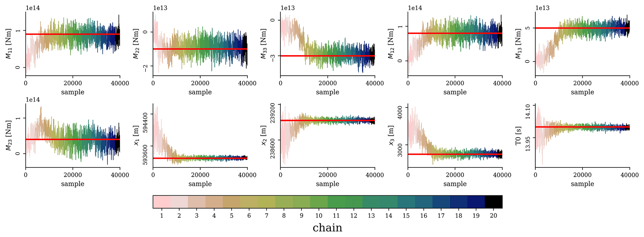
Figure 6 Results of our iterative HMC scheme for a total of 20 chains, each involving 2500 steps, the first 500 of which are discarded as burn-in samples (not shown). The red lines are the true values.

After a total of n HMC chains, we evaluate the posteriors (dark blue box in Fig. 5). This involves the following.

• 8.

  For each of the n posteriors, compute the means m^s ($s=\mathrm{1},\mathrm{\dots },n$). We use these means to generate synthetic recordings and evaluate them against the observed data through determination of the variance reduction (VR).

  $$\begin{array}{}\text{(20)}& \begin{array}{rl}& \text{VR}=\mathrm{1}\\ & -\sqrt{{\displaystyle \frac{{\sum }_{r=\mathrm{1}}^{N_{\mathrm{r}}}{\sum }_{i=\mathrm{1}}^{\mathrm{3}}{\left(u_i\left(x_{\mathrm{r}},t;{\mathit{m}}^s\right)-u_i^{\text{obs}}(x_{\mathrm{r}},t)\right)}^{\mathrm{2}}}{{\sum }_{r=\mathrm{1}}^{N_{\mathrm{r}}}{\sum }_{i=\mathrm{1}}^{\mathrm{3}}{\left(u_i^{\text{obs}}(x_{\mathrm{r}},t)\right)}^{\mathrm{2}}}}}\end{array}\end{array}$$
• 9.

  Define a VR threshold. Posteriors associated with m^s for which the VR exceeds this threshold are used to compute the final posterior distribution.

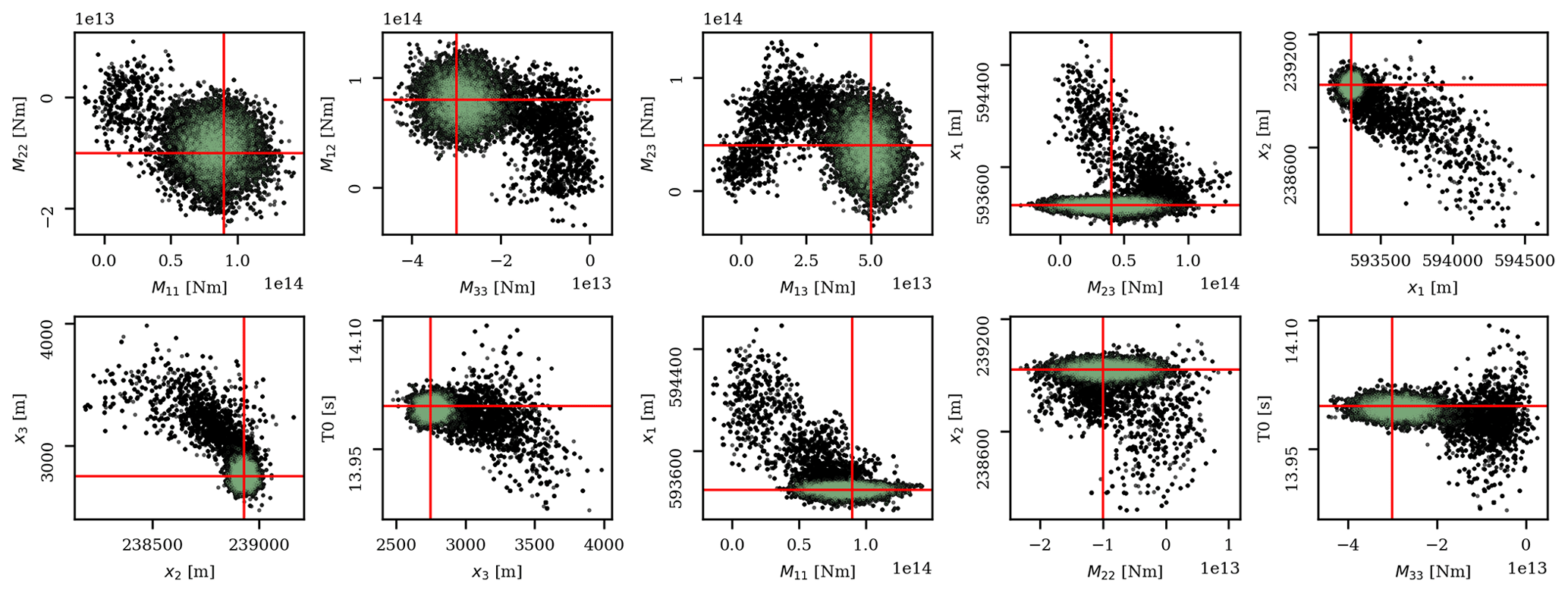
Figure 7 A total of 10 two-dimensional marginal probability densities of the inverted model parameters. Black dots are all the samples given the results from all chains (Fig. 6), whereas the green dots represent the samples from chains that give VR ≥ 85 % of the maximum VR, which then represent our final posterior. The red lines are the true values.

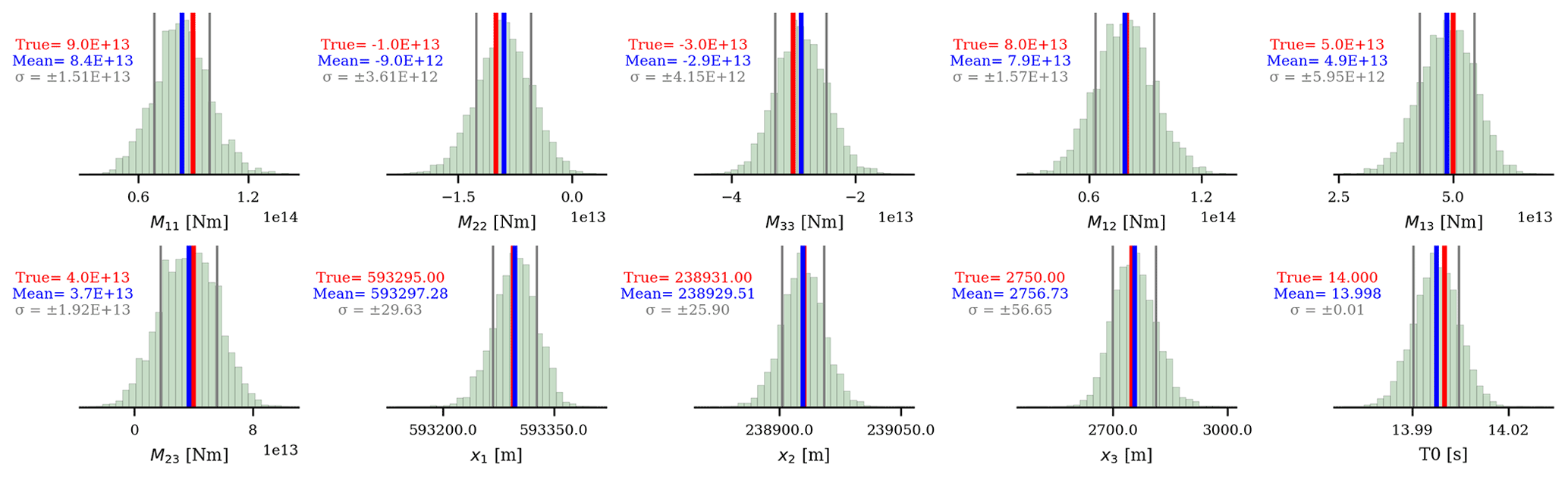
Figure 8 The final marginal posterior distributions (green samples in Fig. 7). The means are represented by the blue lines, and the gray lines are the standard deviations. Red lines are the true values.

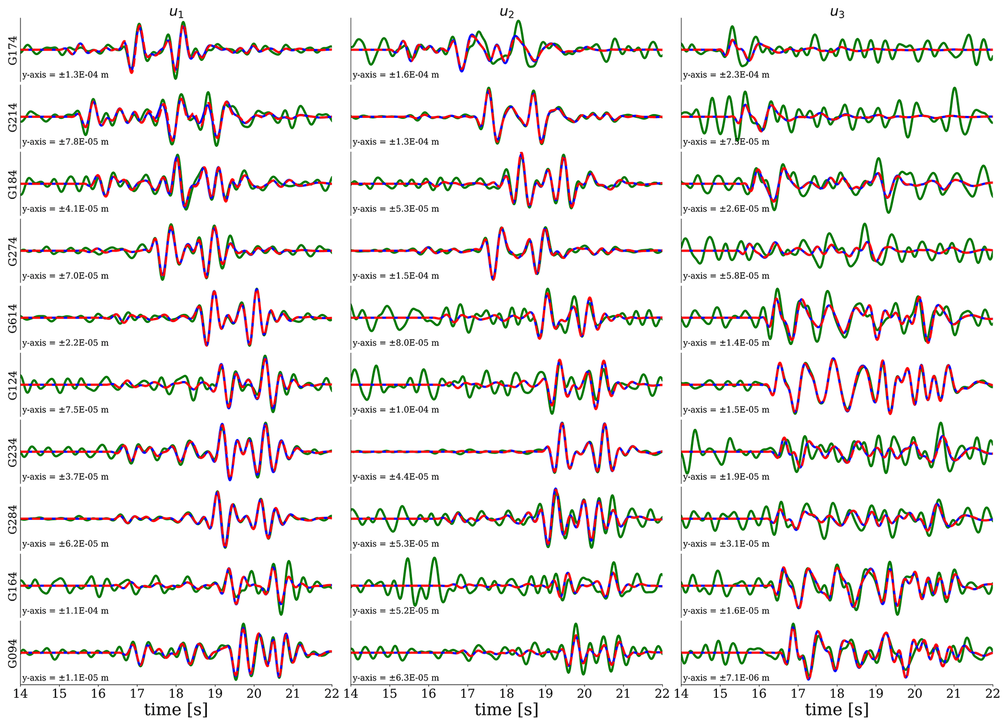
Figure 9 Comparison between the true seismograms (red), observed (true+noise) seismograms (green), and seismograms generated using the final posterior mean (blue).

We use the above workflow to estimate the parameters of the synthetic event shown in Fig. 2. In step 1, we assume a suitable prior of the centroid can be retrieved from the literature (e.g., from Smith et al., 2020, in the case of the seismicity in Groningen). To simulate the fact that this prior may well deviate from the true centroid, we shift this initial centroid prior mean by 600 m in all directions (i.e., with respect to the correct event location). Having the prior mean for the centroid, we follow steps 2 and 3 in the workflow to obtain the other prior means. To encode for a state of ignorance, we set the standard deviation σ_m of each model parameter to infinity, which implies that the last term of Eq. (14) evaluates to 0. The elements of our initial mass matrix are taken from the results of steps 1–3 as explained in the full workflow (step 4), except for those elements that correspond to the centroid; these we set to 300 m. Using the initial prior means and the initial mass matrix, we run 20 chains of the HMC variant. Furthermore, we run 2500 iterations (step 6) for every chain, with the first 500 samples discarded as burn-in samples. After finishing all iterations, the results of each current chain are then used to update the prior means and mass matrix for the next HMC chain (the actual iterative HMC procedure). For each of the 10 model parameters, all 40 000 samples (20 iterations × 200 samples) are depicted in Fig. 6. To obtain our final posterior, we take the results of chains for which the means are associated with seismograms yielding a VR ≥ 85 % of the maximum VR. In detail, the samples from all chains (black dots) and the selected chains (green dots) are depicted in Fig. 7. For the samples of the selected chains, the one-dimensional marginal probability distributions of each of the 10 source parameters are shown in Fig. 8. In Fig. 9, we show the synthetic (observed) seismograms (green), seismograms generated from the final posterior means (blue), and the true noise-free seismograms (red). With the use of a database containing pre-computed elementary seismograms and using the Python code we developed, the entire workflow takes approximately 1 min to finish on a single-core CPU system.

7 The importance of the prior

The above workflow might not be optimal if the initial prior information is “weak” in the sense that the initial centroid prior mean deviates significantly from the true value. This is due to the fact that our forward problem is in essence a nonlinear problem, whereas the adopted linearization (Sect. 4) relies on the assumption of it being only weakly nonlinear. In other words, poor initial centroid priors imply linearization around a location x that deviates too much from the true source location x_a, which may result in the HMC algorithm “getting stuck” in local minima. This problem can be mitigated by running the workflow with multiple initial prior means. Depending on how close each of the initial prior means is to the true values, some chains might get stuck in a local (minimum) mode while others correctly sample the mode containing the global minimum (or global maximum if one considers ρ(m|d)). In the end, the final posterior can be drawn by combining the results of all chains given multiple initial prior means.

To showcase the effect of weak prior information in the context of induced seismicity in the Groningen gas field, we re-use the synthetic earthquake in Fig. 2. However, instead of shifting the initial centroid prior mean by 600 m for all coordinate components, we rigorously shift it by 1 km for each horizontal coordinate. Meanwhile, the depth is set to 3 km, corresponding to the default depth in the KNMI database, because, in application to field data, this database will be our primary source to obtain our priors. To get additional initial centroid prior means, we construct a 2.8 km × 2.8 km 2D grid at a depth of 3 km with a spacing of 700 m centered around the initial centroid prior mean. A pre-test can help in determining the grid spacing. We previously demonstrated that our workflow performs well when the centroid prior means are shifted by 600 m (in all directions) from their true values. This shift corresponds to an absolute deviation of about 1 km. Given the spacing of the constructed grid, assuming that the depth could be around ± 500 m, the maximum total distance is about 700 m, which is then considered safe for the HMC algorithm to sample the mode containing the global minimum.

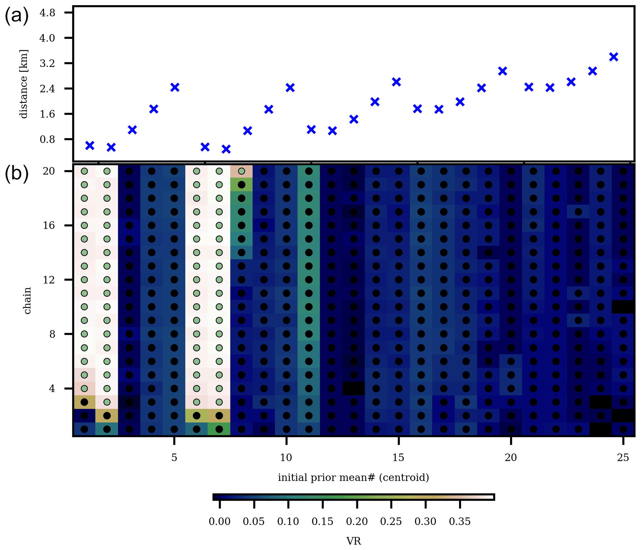
Figure 10 Summary of running the workflow using the 25 initial prior means. The distance between each of the initial centroid prior means and the true centroid is indicated in (a). In (b), we show for each of these initial prior means the VR as a function of chain number (vertical axis). Chains associated with a VR ≥ 85 % of the maximum VR (0.4) are labeled with green dots, whereas chains with a posterior mean yielding seismograms for which the VR does not exceed 85 % are labeled with black dots.

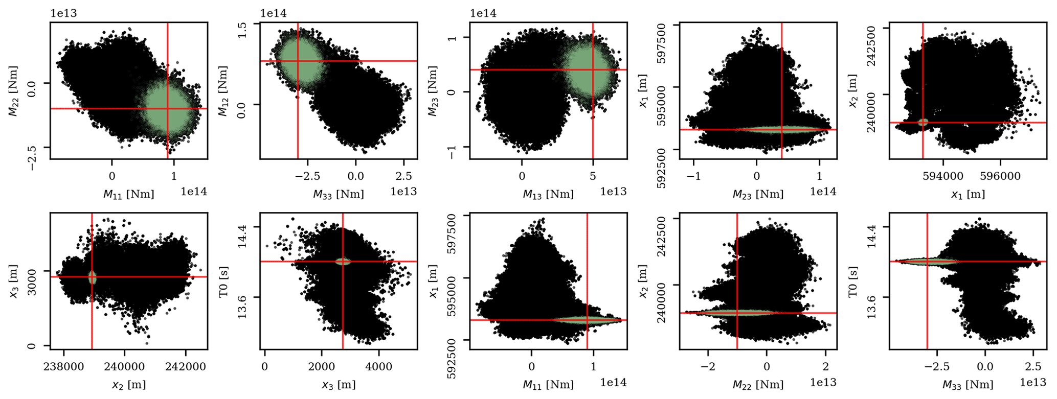
Figure 11 The same 10 two-dimensional marginal probability densities as in Fig. 7. Note that scales on horizonal and vertical axes differ. Black dots are the samples from all chains, whereas the green dots represent the samples from chains with a posterior mean that yields a VR higher than 85 % of the maximum VR. The red lines represent the true values.

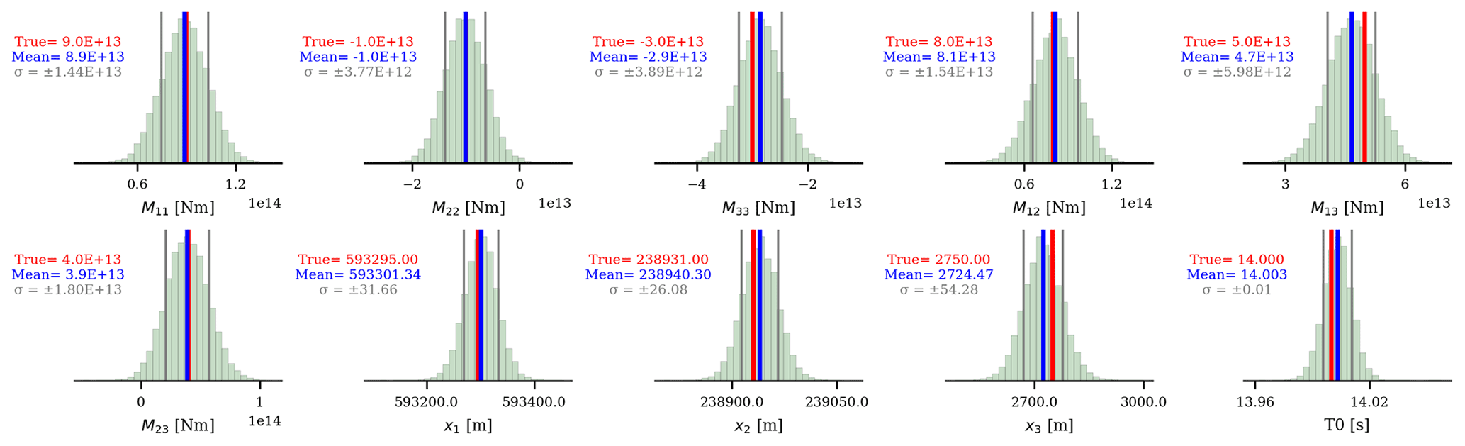
Figure 12 Marginal posterior distributions for each model parameter given the selected chains (depicted as green dots in Fig. 10). The blue lines represent the means, and the standard deviations are represented by the gray lines. The red lines represent the true values.

Overall, given our 5 × 5 horizontal grid, we have 25 initial centroid prior means, each of them being subjected to our workflow. For each workflow run, we use the same model and data uncertainty as in the initial synthetic case. The same applies to the number of chains (20), samples per chain (2500), and burn-in period (500 samples). To reduce the computational time, we run the 25 workflows (associated with 25 initial centroid prior means) simultaneously by parallelizing our code. We subsequently collect the results of each workflow to obtain an estimate of our posterior distribution. The results of this parallelization are summarized in Fig. 10, which highlights the effect of the separation between the centroid prior mean and the true centroid. Using the same threshold as in our initial experiment (VR ≥ 85 % of maximum VR), in Fig. 11, we show all (non-burn-in) samples associated with the selected chains and samples from all chains given the calculated VR. For the selected chains, the marginal probability distribution of each parameter is presented in Fig. 12. As expected, chains with an initial centroid prior mean relatively close to the true centroid converge to the true mode (containing the global minimum). At the same time, chains starting from a centroid further away from the true centroid “got stuck” in a local mode. Fortunately, our VR strategy is still successful in picking appropriate chains, allowing us to obtain an estimate of the posterior distributions.

8 Discussion and conclusions

Using synthetic events, we demonstrate that the proposed probabilistic workflow is able to efficiently estimate the posterior probability of the various parameters describing induced seismic events. A number of caveats need to be made though. First, the synthetic recordings used to test our probabilistic workflow are the result of propagating a wavefield through the very same velocity model as the one used to estimate the posterior (i.e., the velocity model in our probabilistic workflow). In application to field data, this would obviously not be the case. Part of the misfit between modeled recordings and observed recordings would then be the result of discrepancies between the true velocity model and the employed numerical velocity model. Second, and in the same vein, we employed the same code (SPECFEM3D-Cartesian) for generating the synthetic recordings as for modeling the wavefield in the probabilistic workflow. And although this code is known to be rather accurate (Komatitsch and Tromp, 2002), undoubtedly some of the physics describing the actual wavefield propagation are not fully captured by SPECFEM3D-Cartesian. Third, this study does not include an application to field data. This is intentional as our objective is to present a stand-alone workflow that can be applied in any induced seismic setting. Applying a methodology to field recordings of induced seismic events (e.g., in Groningen) would require numerous processing details, which we consider to be beyond the scope of this paper. We are currently drafting a follow-up paper in which we apply the proposed HMC workflow to field recordings of induced seismic events in Groningen.

The aforementioned deviation of the available numerical velocity model from the true subsurface velocities will pose a number of challenges. First, the estimated posterior probability would give a lower bound in terms of the variability of the source parameters: inaccuracies in the velocity model necessarily imply broader posterior probabilities. Second, in the presence of strong anisotropy, the posterior could be adversely affected. In particular, in the case of non-pure shear mechanisms this effect could be significant (Ma et al., 2022). Third, cycle skipping will be particularly hard to tackle in the case that the velocity model is rather inaccurate.

Our workflow includes a systematic approach to obtain meaningful initial priors, which is particularly important for the employed HMC variant: the linearization of the forward problem around the prior mean requires the initial priors to be sufficiently close to the true event location. Furthermore, we show that by using an iterative scheme, we can update the prior mean such that convergence is obtained to a centroid location that allows the estimation of a meaningful posterior. The iterative scheme involves sequentially updating the prior mean of each new HMC chain using the posterior estimate obtained from the previous HMC chain. This approach is based on the suggestion of Fichtner and Simutė (2018) to repeat the Taylor expansion (of the forward problem) for each new sample of the Markov chain. However, we (only) do this every 2500 samples in our case. A brute-force approach to perform the expansion at each step of every chain would render computational costs prohibitively large.

Prior to executing the workflow, one needs to compile a database of the elementary seismograms, which often requires significant computing power. In our case, it took about one day to generate the database using one node of our computer cluster that consists of 24 CPU cores (Intel(R) Xeon(R) CPU E5-2680 v3 at 2.50 GHz) with a total RAM of 503 GB. Once compiled, our workflow can be run efficiently. Using a single-core CPU system, a single run of our workflow with 20 sequential HMC chains takes about 1 min to finish, with each chain consisting of 2500 iterations. In contrast, the computational costs of the Metropolis algorithm (to get the same results) would be much higher, as previously shown (Fichtner and Simutė, 2018; Fichtner et al., 2019). Furthermore, various modifications could be applied to the workflow, such as adding simulated annealing and tempering (Tarantola, 2006), including a step to quantify the error in the input seismograms (Mustać and Tkalčić, 2016) and/or applying a scheme that is able to tune dτ and τ for each HMC run (Hoffman and Gelman, 2014). These modifications could be beneficial, especially when dealing with field observations, which is the subject of future work. We also show that the workflow can be adapted to account for scenarios in which the initial centroid prior mean is rather inaccurate and/or the initial prior is weak. If that is the case, an approach can be adopted in which various iterative HMC workflows, each using a different centroid prior mean as a starting point, are run. Subsequently, using the variance reduction associated with the posterior means of the individual chains as a binary criterion for selecting a chain's samples, a final estimate of the posterior probability can be obtained.

We would like to emphasize that our workflow is, in principle, not limited to inversions of the parameters we use here. We could extend our probabilistic inversion to parameters such as stress drop, velocity, or inverting for finite fault source parameters. Furthermore, it is important to mention that our workflow aims to invert seismic source parameters using seismic surface recordings in a specific frequency range. That is, it is specifically geared towards inverting for induced seismic events. We found that the workflow works well when applied to data with frequencies between 1 and 3 Hz. For higher frequencies, however, some testing might be needed because the nonlinearity between the input data and model parameters increases with increasing frequency.