the Creative Commons Attribution 4.0 License.
the Creative Commons Attribution 4.0 License.
 | 10 Jan 2022
De-risking the energy transition by quantifying the uncertainties in fault stability
David Healy
Stephen Paul Hicks
The operations needed to decarbonize our energy systems increasingly involve faulted rocks in the subsurface. To manage the technical challenges presented by these rocks and the justifiable public concern over induced seismicity, we need to assess the risks. Widely used measures for fault stability, including slip and dilation tendency and fracture susceptibility, can be combined with response surface methodology from engineering and Monte Carlo simulations to produce statistically viable ensembles for the analysis of probability. In this paper, we describe the implementation of this approach using custom-built open-source Python code (pfs – probability of fault slip). The technique is then illustrated using two synthetic examples and two case studies drawn from active or potential sites for geothermal energy in the UK and discussed in the light of induced seismicity focal mechanisms. The analysis of probability highlights key gaps in our knowledge of the stress field, fluid pressures, and rock properties. Scope exists to develop, integrate, and exploit citizen science projects to generate more and better data and simultaneously include the public in the necessary discussions about hazard and risk.
- Article
(9072 KB) - Full-text XML
- BibTeX
- EndNote


1.1 Rationale and objectives
Faults in the crust slip in response to changes in stress or pore fluid pressure, and the source of these changes can be either natural or anthropogenic. Estimating the likelihood of slip on a particular fault for a given change in loading is critical for the industrial operations of the energy transition, especially geothermal energy and carbon sequestration and storage (CCS). The target formations of these operations are nearly always faulted and fractured to some degree, and experience from waste water injection in the USA shows how even small changes in pore fluid pressure can trigger frequent seismic slip on these faults, with significant and widespread impacts on society (e.g. Ellsworth et al., 2016; Hincks et al., 2018; Hennings et al., 2019).
Stephenson et al. (2019) have shown how quantitative analysis of the subsurface is one of the key contributions that geoscientists can make to decarbonizing energy production to meet national and international targets (e.g. CCC, 2019; IPCC, 2018). This includes the systematic geomechanical characterization of rock formations, better understanding of fluid flow in fractured rocks, and the need for pilot projects to explore the scaling of behaviours from the laboratory to the field. Perhaps the most important aspect is to understand the public attitudes to subsurface decarbonization technology (Stephenson et al., 2019; Roberts et al., 2021). Several recent studies have addressed the uncertainties in subsurface structural analysis of faulted rocks (Bond, 2015; Alcalde et al., 2017; Miocic et al., 2019). In this paper, we extend this work to specifically include fault stability and argue that in order to simultaneously address public concerns and assess the viability of different schemes, we need a more rigorous approach to de-risking subsurface decarbonization activities, especially where these involve changes in load on faulted rocks.
Useful measures of fault stability include slip and dilation tendency (Ts and Td, respectively) and fracture susceptibility (Sf, the change in fluid pressure to push effective stress to failure). These measures are defined as functions of the in situ stress, the orientation of the fault plane, and (in the case of Sf) rock properties. It is widely recognized that the inputs for the prediction of stability are always uncertain to varying degrees: for example, the vertical stress component of the in situ stress tensor can often be quite well constrained (to within 5 %) from density log data, whereas the maximum horizontal stress is generally much harder to quantify. To improve and focus our predictions of fault stability in the subsurface, we need to accept and incorporate these uncertainties into our calculations. In this paper, we describe and explore a statistical approach to fault stability calculations and then apply these methods to examples in geothermal energy in both low- and high-enthalpy settings.
The specific aims of this paper are as follows:
-
to describe and explain the response surface methodology (RSM) and show how it can be applied to the probabilistic estimation of fault stability using a range of different measures;
-
to explore how the main variables – in situ stress, fault orientation and rock properties – relate to the different measures of fault stability (Ts, Td and Sf) using synthetic (i.e. artificial) data;
-
to use case studies of active and proposed geothermal projects with publicly available data to illustrate the method and then highlight the relationships between our known but uncertain input data and the predicted risk of fault slip.
1.2 Importance and previous work
Small changes in stress or fluid pressure (e.g. a few MPa) from human activities can have significant consequences for fault stability (Raleigh et al., 1976). For example, waste water injection from hydraulic fracturing (“fracking”) operations has led to dramatic increases in seismicity in Oklahoma since 2009 (Hincks et al., 2018) and in Texas since 2008 (Hennings et al., 2019; Hicks et al., 2021). The precise mechanical cause(s) of this seismicity is the subject of some debate and could be due to either “direct” pore fluid pressure transfer to basement-hosted faults leading to a reduction in effective stress or “indirect” poroelastic effects at a distance (Ellsworth et al., 2016; Goebel et al., 2019). The concept of critically stressed faults in the crust (Townend and Zoback, 2000), where relatively high permeability serves to maintain near-hydrostatic pore pressures, is consistent with the idea that only minor perturbations in loading can have dramatic consequences, even in areas of apparently low seismicity and, implicitly, low background tectonic loading.
In densely populated areas such as the UK, public support for, and confidence in, subsurface operations are key. Hydraulic fracturing operations for shale gas in Lancashire (UK) were stopped after earthquakes were triggered by fluid injection (Clarke et al., 2019). Triggered felt seismicity has already been reported at the United Downs deep geothermal pilot in Cornwall (Holmgren and Werner, 2021). Note that in both of these cases fracturing and/or fault slip are intrinsic to the success of the operation as they are needed to enhance fluid flow, and therefore earthquakes are inevitable. In detail, microseismicity (i.e. M<2) is inevitable, but it is important to understand whether felt (i.e. M>2) seismicity can be forecast ahead of time. Furthermore, many sites for energy transition projects in the UK are located in (beneath) areas of extreme poverty and social deprivation, both rural (e.g. Cornwall, South Wales) and urban (e.g. Glasgow), and therefore the risks from these projects fall disproportionately on the less well off (Nolan, 2016; McLennan et al., 2019). To begin to address these complex issues, we need to quantify which faults are more or less likely to slip in response to induced changes in loading. One approach is to analyse data during subsurface operations and attempt to manage the consequences (e.g. Verdon and Budge, 2018). An alternative approach, and the one taken in this paper, is to look at the bigger picture before operations commence and reduce risk from the outset.
Various measures have been proposed to quantify the propensity or tendency of a given fault to slip (or open) in a known stress field. The following methods are based around an assumption of Mohr–Coulomb (brittle-plastic) failure, which has been shown to capture the key aspects of faulting in the upper crust. Slip tendency (Ts) was introduced by Morris et al. (1996) and is the simplest measure of fault stability, defined as follows:
where τ is the shear stress and σn is the normal stress acting on the fault plane. These stress components in turn depend on the principal stresses and the orientation of the fault plane (see Lisle and Srivastava, 2004, for details). In the absence of cohesion, if the slip tendency on a fault equals or exceeds the coefficient of sliding friction, then the fault can be deemed “unstable”. This dimensionless index embodies the key mechanical principle underlying Mohr–Coulomb shear failure: as the shear (“sliding”) stress acting on a fault plane rises in relation to the normal (or “clamping”) stress, the fault approaches failure and will slip. Slip tendency allows us to compare what we know about the stress state on a fault (τ, σn) with what we know about the rock properties (coefficient of sliding friction, μ). Dilation tendency (Td) has been defined to describe the propensity for a fault to open (or dilate) in a given stress regime:
where σ1 and σ3 are the principal stresses of the in situ stress tensor (Ferrill et al., 1999).
Most rocks in the upper crust are porous and permeable to some degree, and fault rocks are no exception, so these rocks are generally saturated with fluid. This implies that we should include pore fluid pressure and the concept of effective stress in our assessment of fault stability. Fracture susceptibility (Sf) is the change in pore fluid pressure needed to push a stressed fault to failure (Streit and Hillis, 2004) and is defined by the following equation:
where Pf is the pore fluid pressure at the fault and C0 is the cohesive strength (or cohesion; see Fig. 1b).
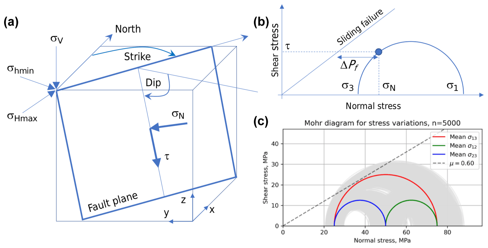
Figure 1(a) Schematic block diagram of a fault plane showing the terminology used in this paper. Also shown are the Cartesian and geographic reference frames and the Andersonian principal stresses. (b) Mohr diagram for a given state of stress (blue semicircle) with normal (σn) and shear stresses (τ) marked for a selected fault plane orientation (blue dot). Failure envelope for frictional sliding (cohesion = 0) is also shown as a straight blue line. (c) Mohr diagram depicting one of the key issues tackled in this paper: given uncertainty in the input stress values (grey Mohr circles for the variation around the average principal stresses in red, blue, and green), what is the probability of failure; i.e. what percentage of all of these stress states will intersect the failure envelope?
Previous applications of these three measures of fault stability – Ts, Td, and Sf – cover the full spectrum of rock types and stress fields, from basins to basement and from extensional, contractional and wrench tectonic settings. Applications within the domain of the energy transition include examples from geothermal energy (both shallow and deep) and CCS. The original definition of fracture susceptibility by Streit and Hillis (2004) was concerned with safe injection limits for CO2 in potential reservoirs in Australia. Moeck et al. (2009) used slip tendency to quantify the relative stability of different fault sets in different horizons in a geothermal reservoir in the North German basin, and Barcelona et al. (2019) used a similar method for Copahue geothermal reservoir in Argentina. For CCS, Williams et al. (2016, 2018) have used slip tendency analyses of faults in potential sandstone reservoirs on the UK continental shelf, including the North Sea and East Irish Sea basins. The links between subsurface fluid flow, seismicity, and fault stability have recently been explored by Das and Mallik (2020) for the Koyna earthquakes in India and by Wang et al. (2020) for strike-slip faults in the Tarim Basin of China.
Probabilistic approaches to fault stability have been adopted by various workers. In risking CO2 storage for an oil reservoir in the Williston basin, Ayash et al. (2009) used a features, events, and processes (FEP) approach to constrain the likelihood of occurrence of fault slip (based on slip tendency) and the severity of the consequences, with their product defined as the risk. Rohmer and Bouc (2010) used RSM to assess cap rock integrity for tensile or shear failure above deep aquifers in the Paris basin targeted for the storage of CO2. Coupled RSM and Monte Carlo approaches to fault stability have been used by Chiaramonte et al. (2008) and Walsh and Zoback (2016), following their initial application in the field of wellbore stability by Moos et al. (2003). This fault slip potential (FSP) method developed by Stanford (e.g. Chiaramonte et al., 2008; Walsh and Zoback, 2016) calculates the response surface for fracture susceptibility, with the in situ stress tensor calculated by inversion of abundant seismicity data (focal mechanisms), and then uses a Monte Carlo simulation to generate cumulative distribution functions (CDFs) of conditional probability of slip defined with reference to an arbitrary pore pressure perturbation (ΔPf=2 MPa, in the case of Walsh and Zoback, 2016). Note that FSP assumes cohesionless faults (C0=0) and hydrostatic pore fluid pressure and that conditional probability in this sense refers to the fact that we do not know where any particular fault is with respect to the seismic cycle.
1.3 Conventions and layout for this paper
In the sections below, we describe the underlying equations for measuring fault stability and then show how we can use response surface methodology (RSM) from engineering to explore the consequences of uncertainties in the input variables. After assessing the quality of the solutions obtained from RSM, we then apply a brute force Monte Carlo (MC) approach to generate cumulative distribution functions (CDFs) of the different measures (Ts, Td and Sf). The case studies use published, publicly available data to constrain the input variable distributions and then a combined RSM–MC approach is used to explore the uncertainty in fault stability in different settings.
In this paper, compressive stress is reckoned positive, with σ1 as the maximum compressive principal stress and σ3 as the minimum principal stress. Stress states and fault regimes are assumed to be Andersonian, with one principal stress vertical, although the underlying model and code could be changed to incorporate non-Andersonian stress states with the addition of extra variables for the stress tensor orientation (Walsh and Zoback, 2016). The likelihood of slip on a fault is assessed in the framework of Mohr–Coulomb failure, with or without cohesion (Jaeger et al., 2009). Fault orientations are quantified as strike and dip following the right-hand rule: with your right hand flat on the fault plane and fingers pointing down dip, the right thumb points in the direction (azimuth) of strike. The relationship between the geographical and cartesian reference frames follows a north east down convention. Figure 1 depicts the key terms and elements used in the analysis, and Table 1 contains a list of terms and symbols used with units where appropriate.
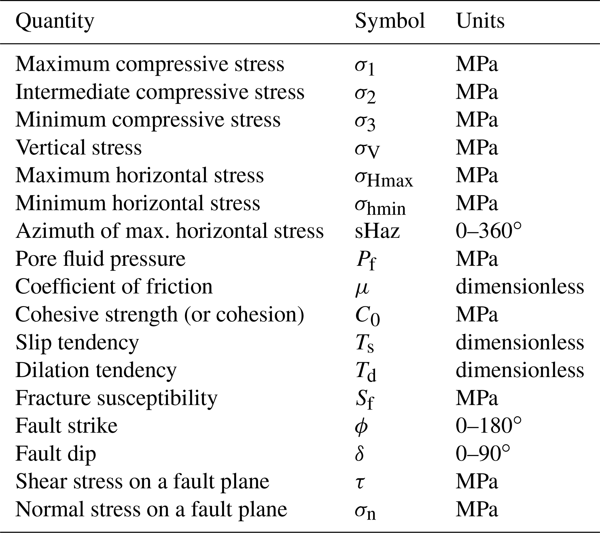
Table 1List of terms and symbols used in this paper, with units where appropriate.
2.1 Introduction to response surface methodology (RSM)
RSM is widely used in engineering and industry along with a design of experiments approach, and often employed to optimize a specific process of interest – e.g. to maximize the yield of a reaction given the input variables of pressure, temperature, reactant mass. RSM is a large and growing field and is best considered as a toolbox of different methods with a common mathematical basis. The governing equations for RSM were derived by Box and Wilson (1951). The core idea is that a response y can be represented by a polynomial function of a number (q) of input variables x1−xq:
Each of the q input variables can be represented by either a discrete set of measurements made in the laboratory (or field) or drawn from appropriate statistical distributions (normal or Gaussian, skewed normal, Von Mises, etc.). The simplest polynomial function that relates y and x is a linear one:
where βq is the coefficients (to be determined), yi is the set of observations of the response (), and xij is the set of input variables (). ϵ is the experimental error, and the number of “observations” N>q the number of input variables. This is therefore a multiple regression model linking the response y to more than one (i.e. multiple) independent variable, x.
A more complex polynomial relationship is the following quadratic form:
This second-order multiple regression model contains all the terms of the linear (first-order) model but also extra terms for the squares and cross-products of the input variables (second and third terms on the right-hand side, RHS, of Eq. 7).
To define a response surface, either linear or quadratic, we need to calculate the values of the βq coefficients. We can rewrite the key equations in matrix form:
where y is an (N×1) vector of observations (or calculations), X is an (N×k) matrix of input variable values (), and β is a (k×1) vector of regression coefficients. We solve this system of equations using the standard linear algebra technique of least-squares regression (Myers et al., 2016):
The response surface (linear or quadratic) is then defined by
The values used in X are chosen to efficiently span the parameter space. A typical sampling design for X is called the 3q model, with 3 values of each variable, usually the minimum, mean (or mode), and maximum. In practice, coded variables are used in X where the absolute values for the minimum, mean, and maximum of each variable are scaled to −1, 0, and +1, respectively, and then scaled back when the response surface is used in the Monte Carlo simulation (Myers et al., 2016).
The response surface, i.e. the set of β coefficients, is defined using a limited number of sample points, depending on the chosen sample design (3q in the examples used in this paper; other variants exist; see Myers et al., 2016, for details). To explore the possible variations of a response more fully, we use a Monte Carlo (MC) approach of pre-defined size (NMC=5000 in the examples in this paper). The MC simulation uses the response surface calculated from the design points to calculate the responses for NMC combinations of input variables drawn from their distributions. This produces a statistically viable ensemble of response values from which we can infer the probability of the response with respect to a chosen threshold.
With respect to fault stability, we can use RSM to produce a parameterized relationship – the response surface in q dimensions – between a stability measure of interest and the q input variables. In the case of slip tendency Ts, we can rewrite the components of Eq. (1) in terms of the measurable input quantities as follows:
where l, m, and n are the direction cosines of the normal (pole) to the fault plane given by
where φ is the fault strike and δ is the fault dip in a north east down reference frame (Allmendinger et al., 2011).
All terms on the RHSs of Eqs. (11)–(13) are uncertain to some degree; therefore, estimating the uncertainty of Ts and (just as importantly) the key controls on the uncertainty of Ts in terms of these input variables is non-trivial. This difficulty in estimating and visualizing possible variations in our estimates of Ts is exacerbated by the recognition that each of the input variables may be distributed differently: some quantities (e.g. the principal stresses) may follow normal (Gaussian) statistics, whereas others (e.g. strike, dip, sHmax azimuth) may follow Von Mises distributions. In the case of fracture susceptibility (Sf, Eq. 3), it is complicated even more by the addition of three further input variables for friction, cohesion, and pore fluid pressure. Measurements or calculations of coefficients of friction and cohesive strength often display asymmetric or skewed distributions (skewed high or low), and this adds further complexity to the task of estimating and constraining fault stability from the data at hand.
2.2 Worked example one: slip tendency from synthetic input data
The calculations presented in this paper were all performed with the custom pfs (probability of fault slip) package, which was written by the first author (David Healy) in Python 3 and is freely available on GitHub (see Code Availability, below).
The first example calculates a response surface for slip tendency (Ts) from q=6 input variables: the magnitudes of the three principal stresses of the in situ stress tensor (σ1, σ2, σ3) assumed Andersonian with one principal stress vertical, the azimuth of the maximum horizontal stress (sHaz), and the strike and dip of the fault plane. We build a response surface using a 3q design, i.e. three data points for each variable (minimum, mean, and maximum) and for Ts, q=6. This means we calculate the response surface from 36=729 data points. This response surface is then used in a Monte Carlo simulation (NMC=5000) to generate a CDF of Ts values for the fault. The specific Python code to run this example in the pfs package is wrapped in a Jupyter notebook available on GitHub (WorkedExample1.ipynb).
The first task is to define the distributions of the input variables. In pfs, examples are shown for normal, skewed normal, and Von Mises (circular normal) distributions, but other statistical distributions are allowed. Table 2 and Fig. 2 describe the ranges and statistical moments of these distributions for each input variable. For this example, the normally distributed principal stresses are defined with a variation (standard deviation) of 5 % of their central (mean) value, and the Von Mises distributions of the azimuthal variables (sHaz, strike, and dip) all have κ=200 to model their dispersion about their mean. The fault of interest strikes 060∘ and dips 60∘ to the south (right-hand rule). The key questions to be addressed by this example are as follows.
-
Given these uncertainties in the input stresses and orientation data, how does the estimation of Ts vary? What is the range and the mode?
-
Which variables exert the greatest (and least) control on the predicted variation in Ts?
We compare a calculated linear response surface with a quadratic response surface using a normal probability plot of residuals (Fig. 3). These residuals are the differences between the values of Ts derived from the observations (taken from the input distributions shown in Table 2 (upper) and Fig. 2), and the calculated values of Ts using the β coefficients derived by least-squares regression, i.e. the response surface. The adjusted R2 value for the quadratic second-order model is significantly better than that for a linear first-order model, and we use quadratic models throughout the rest of this paper. More detailed inspection of the quality of fit between the response surface and the observations is possible, including analysis of variance, main effects plots, and the use of t statistics for each input variable to quantify their significance to the definition of the β coefficients (Myers et al., 2016). In practice, visualizing sections of the response surface for individual variables is generally sufficient (see below; Moos et al., 2003; Walsh and Zoback, 2016).
Table 2Table of input variable distributions for the synthetic models in worked examples one and two.
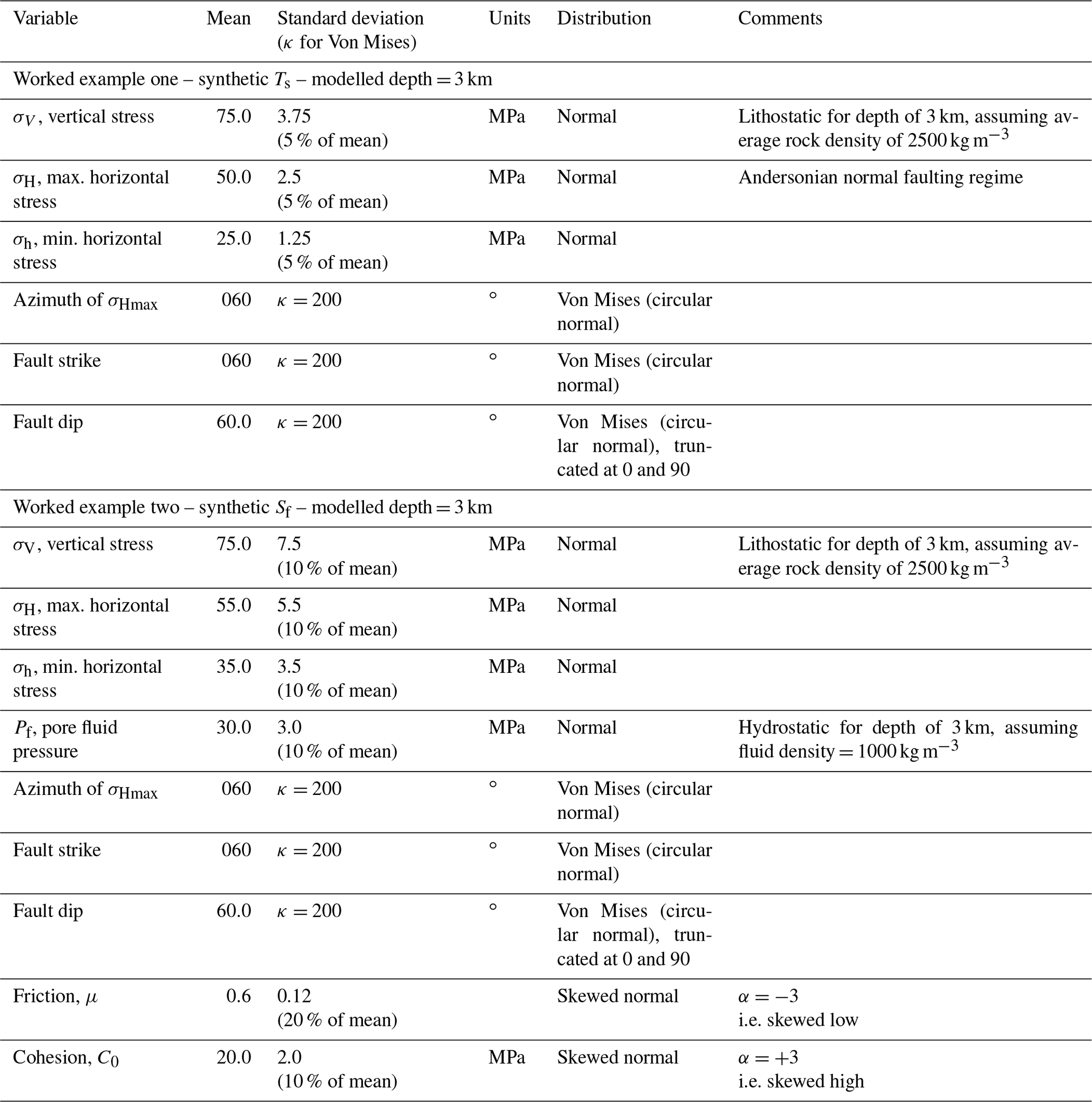

Figure 2Histograms of input variables used to calculate slip tendency Ts for the synthetic distributions shown in Table 2 (worked example one). Input value distributions are shown in blue. The calculated response surface is shown in red.
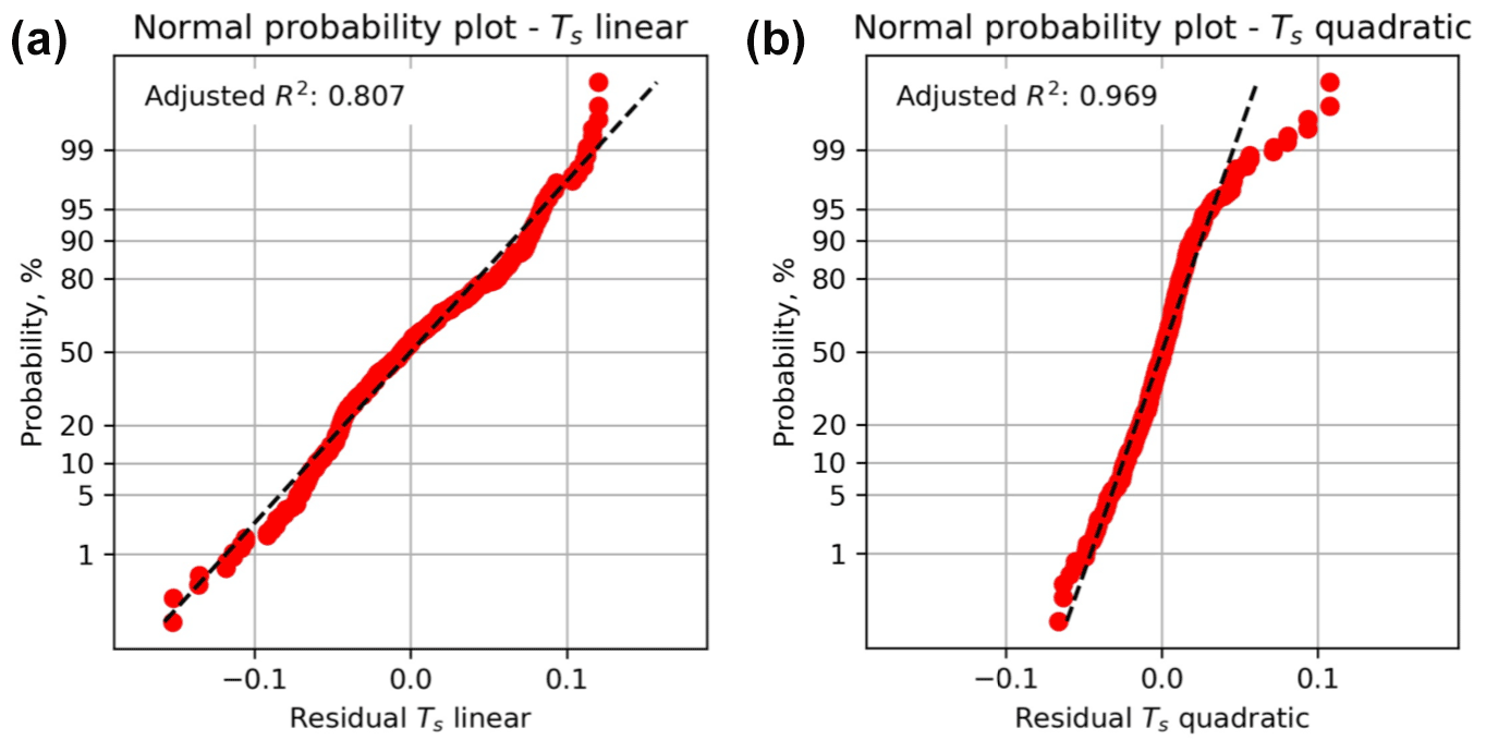
Figure 3Residual plots for linear and quadratic response surfaces for slip tendency (Ts) using synthetic data from worked example one. The quadratic fit has a higher value of the adjusted R2 parameter and is therefore deemed to be better in this case.
Having generated the quadratic response surface for Ts for these input distributions, we can now use it to perform a Monte Carlo (MC) simulation with the aim of generating a statistically viable ensemble from which we can infer the probability of Ts exceeding a critical value of sliding friction. The results from the MC analysis of Ts are shown in Fig. 4. The histogram of all values of Ts shows a symmetrical and rather narrow distribution with a modal value of about 0.56 (Fig. 4a). The CDF of all values of Ts also shows this narrow and symmetrical distribution (Fig. 4b).
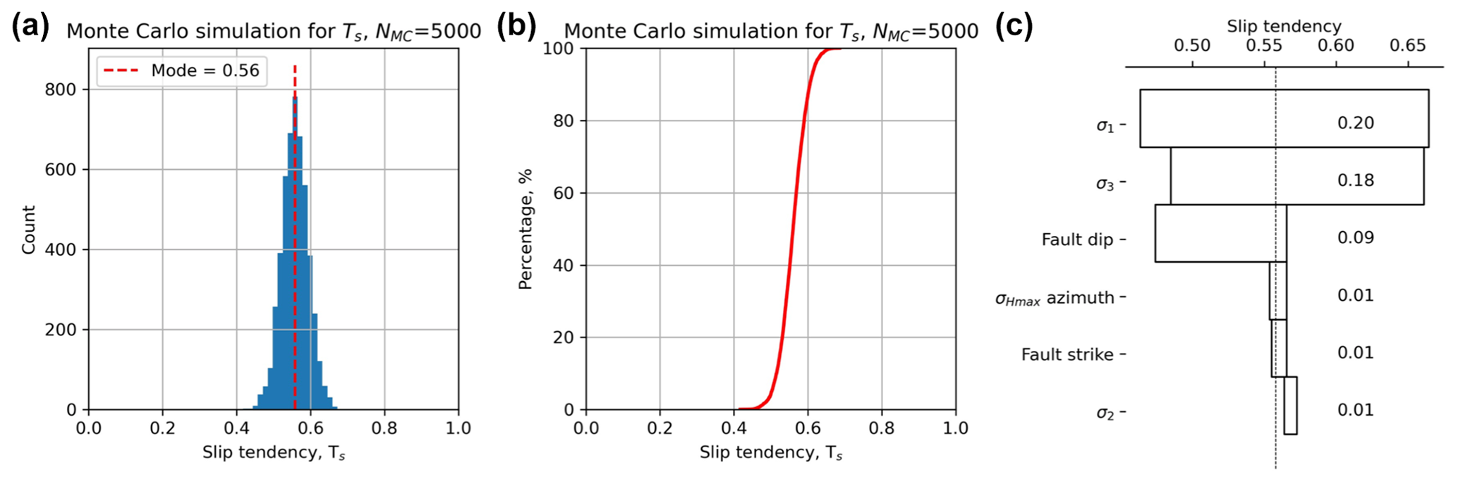
Figure 4Output from Monte Carlo simulation (NMC=5000) of slip tendency (Ts) calculated using a quadratic response surface from synthetic input data in worked example one. (a) Histogram of calculated Ts values, in this case showing a quasi-normal distribution with a mode of ∼ 0.55. (b) Cumulative distribution function (CDF) of calculated Ts values, showing the range in values from ∼ 0.4 to ∼ 0.7. (c) Tornado plot showing relative sensitivity to the input variables. The vertical dashed line shows the modal (most-frequent) value of Ts from the MC ensemble.
A response surface of more than two variables is not easy to visualize. One approach is to take sections through the surface at specific values of all but one variable and graph that. The red lines shown in Fig. 2 depict the response surface for that variable with all other variables held at their mean values. Thus, the red line in Fig. 2a shows the variation in Ts as σ1 varies with all other variables (σ2, σ3, sHaz, φ, and δ) held at their mean values. There is a clear positive correlation of increasing Ts with increasing σ1, as expected from the definition of Ts and its underlying dependence on differential stress (); the clear negative correlation of Ts with σ3 shown in Fig. 2c confirms this. Many of the response surface sections shown in Fig. 2 are quasi-linear, but some are not: in particular, the dependencies of Ts on sHaz, strike, and dip are all non-linear, and this further justifies the selection of a second-order quadratic response surface model.
A useful way to visualize the results from the response surface calculated by the MC simulation is the tornado plot shown in Fig. 4c. Here the ranges of Ts for each input variable (shown as red lines over the histograms in Fig. 2) are plotted to show the relative sensitivity of Ts to each variable. Variables are ranked from the largest range at the top to the lowest range at the bottom. Again, the core dependence of Ts on differential stress (=σ1 – σ3) is apparent, with σ1 and σ3 ranked highest in the plot. Interestingly, fault dip is ranked the next highest in terms of sensitivity, and this reflects the geometry of this particular example. The Andersonian stress regime is for normal faulting with σ1 vertical, σ2 is oriented parallel to fault strike (sHaz = strike = 060∘), and the fault dips at 60∘. This fault is therefore ideally oriented for slip in this stress field. Small changes to dip will influence the ratio of τ to σn, and therefore Ts.
We can use a Monte Carlo approach to explore these sensitivities in more detail. Given the shape of the response surface sections shown in Fig. 2 and the ranking of variables in Fig. 4c, we can quantify how more or less variation in the inputs will affect the predicted Ts. Figure 5 shows the results of this sensitivity analysis for σ3 and fault dip. The most significant effect on the CDF of Ts is produced by increasing the variation in σ3 to 20 % of the mean. This level of uncertainty for the minimum stress is not unreasonable in real-world scenarios (see Sect. 3). Increased uncertainty in σ3 at this level leads to a ∼ 20 % chance of Ts being in excess of 0.7 (p=0.8 for from Fig. 5a). Increased uncertainty in fault dip is achieved by varying the dispersion parameter κ of the Von Mises distribution (lower values of κ = more dispersed). Very disperse distributions of fault dip with κ = 20 only change Ts by <0.1.
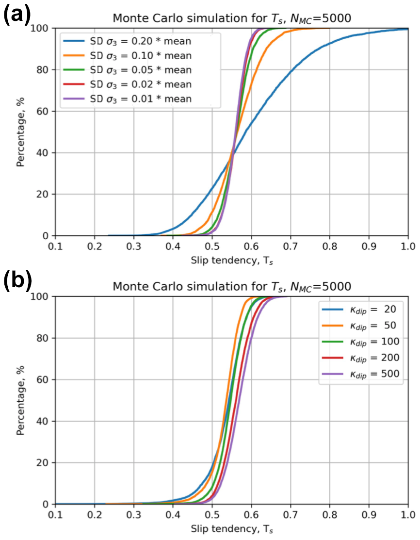
Figure 5Output from Monte Carlo sensitivity tests for slip tendency (Ts). (a) Effect of variation in standard deviation of the least principal stress, σ3. (b) Effect of variation in dispersion (κ parameter of the Von Mises distribution) of fault dip.
2.3 Worked example two: fracture susceptibility from synthetic input data
We can explore variations in predicted fracture susceptibility using the same principles as for slip tendency but adjusted by incorporating three new variables as required by Eq. (3) – pore fluid pressure, friction coefficient, and cohesion (code in GitHub: WorkedExample2.ipynb). The number of variables q is now 9, and therefore the design space used to compute the response surface is 3q=39 = 19 683 data points. In practice this means a slower runtime, but it still only takes a few minutes on a modern processor.
For this example, we use the same stress tensor as for the Ts example, with σ1 as the maximum principal stress and vertical, i.e. an Andersonian normal fault regime for a depth of approximately 3 km. We constrain the in situ pore pressure with a symmetrical normal distribution with a mean value of 30 MPa, which is approximately hydrostatic for a depth of 3 km, and with a variation of 10 % of this mean. Friction is constrained by a skewed normal distribution with a mode of 0.56 and skewness parameter , i.e. skewed towards lower values. This shape of distribution for friction coefficients is consistent with previous studies (e.g. Moos et al., 2003; Walsh and Zoback, 2016) but is open to question (see Sect. 4). Similarly, for cohesion we use a skewed normal distribution with a mode of 21 MPa and , i.e. skewed towards higher values, again consistent with previous work. These input variable distributions are documented in Table 2 (lower) and shown in the histograms of Fig. 6.
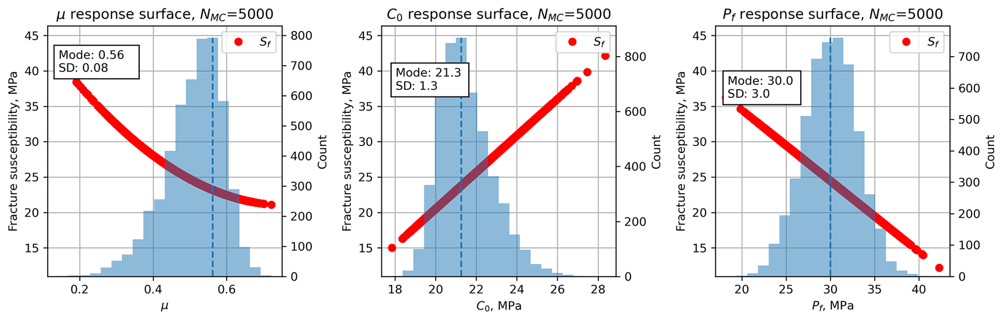
Figure 6Histograms of the input variables (blue), in addition to those shown in Fig. 2, used to calculate fracture susceptibility (Sf) for the synthetic distributions of worked example two shown in Table 2. Note the skewed (asymmetric) distributions for μ and C0.
We calculate a quadratic response surface and use a Monte Carlo simulation (NMC=5000) to generate the ensemble summarized in Fig. 7. The mode of the distribution of Sf is 21.7 MPa, meaning that, on average, an increase in pore fluid pressure of about 22 MPa above the average in situ value of 30 MPa is needed to push the effective stress state to Mohr–Coulomb failure. The histogram in Fig. 7a is approximately symmetrical, perhaps with a slight skewness to higher values, and this is reflected in the CDF shown in Fig. 7b. The distribution is overwhelmingly positive, meaning that this fault is almost unconditionally stable for any change in pore fluid pressure at these conditions. The response surface sections for μ, C0, and Pf shown in Fig. 6 (red lines) all show a strong influence on the fracture susceptibility, and these are confirmed in the tornado plot of Fig. 7c. Pore fluid pressure exhibits a negative correlation with Sf (Fig. 6c), which is consistent with the general principle of effective stress: i.e. if the original in situ pore pressure is already high, it only takes a small perturbation (small ΔPf=Sf) to promote sliding failure. The response to changes in μ and C0 is more interesting (Fig. 6a and b). For this magnitude of cohesion, the effect of cohesion on Sf is greater than that of μ (C0 ranks higher than μ in the tornado plot, Fig. 7c), and the dependence of Sf on μ is negative. However, this relationship is not general as will be shown in the case study for the Porthtowan Fault Zone (see below).
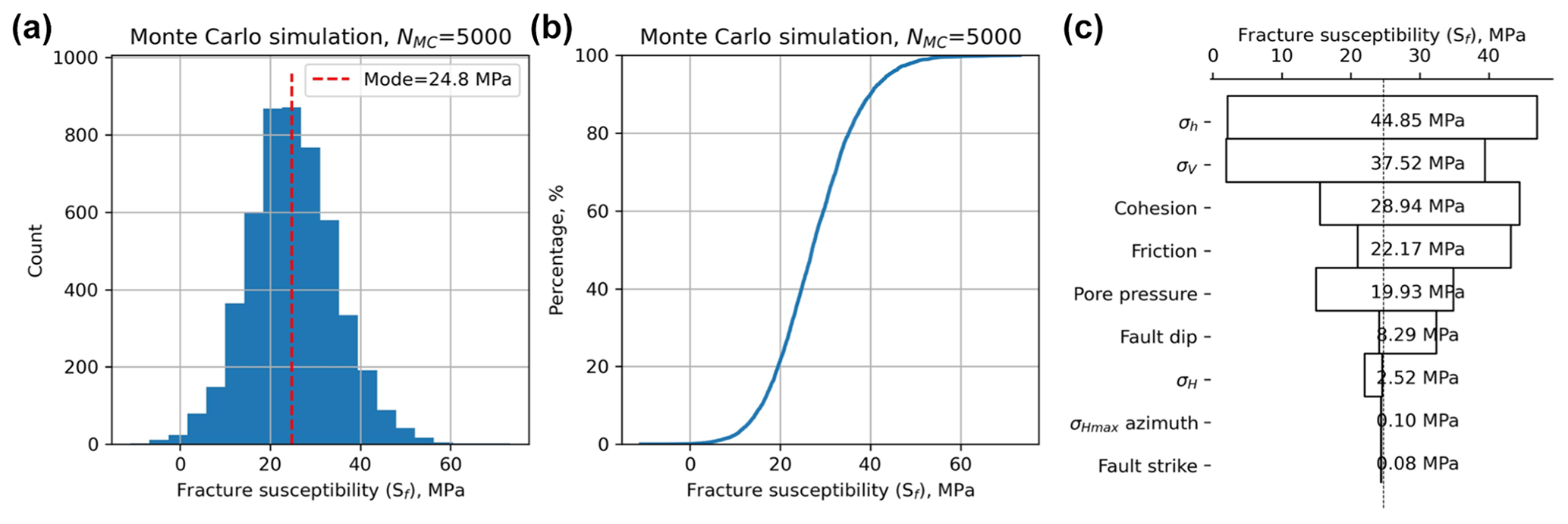
Figure 7Output from Monte Carlo simulations (NMC=5000) of fracture susceptibility (Sf) calculated using a quadratic response surface from synthetic input data in worked example two. (a) Histogram of calculated Sf, showing a quasi-normal distribution with a mode of 21.7 MPa. (b) Cumulative distribution function (CDF) of calculated fracture susceptibility, showing the range in values from just less than 0 to about 60 MPa. (c) Tornado plot of relative sensitivities of the input variables used to calculate fracture susceptibility (Sf).
The relative asymmetries of the skewed normal distributions for μ and C0 have already been noted. Given their significant effect on Sf (high ranking in the tornado plot, Fig. 7c), it is useful to explore how the skewness of these distributions might influence Sf. Figure 8 shows the results of repeated Monte Carlo sensitivity tests for μ (Fig. 8a, b) and C0 (Fig. 8c, d). For friction, a positive skewness to higher values (α>0) would tend to reduce Sf – i.e. faults would be less stable. For cohesion, the opposite is true – a negative skewness (α<0) would make faults less stable to changes in Pf. These asymmetries are opposite to the ones used in the main worked example two and used by other workers (see Sect. 4). Widening the distributions for μ or C0 by increasing their standard deviations (and retaining the original α values) tends to broaden the distribution of predicted Sf with asymmetry to higher (i.e. more stable) values.
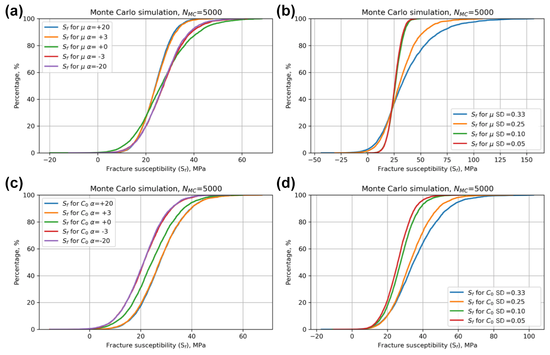
Figure 8Sensitivity of fracture susceptibility (Sf) to variations in μ and C0 for worked example two. Note the changes in scale along the x axis between the plots.
The case studies have been chosen to illustrate how a combined RSM–MC approach that can be used to estimate the probability of slip on one or more faults. Selected specific aspects of the modelling and the visualization of results are emphasized in each case study. Figure 9 shows a map of the UK with the case study areas marked, together with the locations of instrumentally recorded earthquakes and their focal mechanisms (Baptie, 2010). Also shown are data from the World Stress Map database of 2016 (Heidbach et al., 2018) indicating the orientation of the maximum horizontal stress. A basic observation from this map is the level of complexity and heterogeneity in the present-day seismotectonics of the UK, reflecting the variation in the subsurface geology. However, there is a broad prevalence of NW–SE-trending σHmax directions and strike-slip earthquake mechanisms.
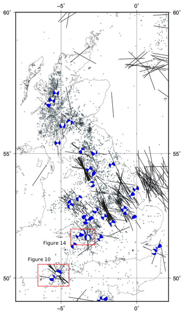
Figure 9Map of most of the UK showing the locations of the selected case studies (red rectangles). Also shown are epicentres of seismicity (dots; British Geological Survey (BGS) catalogue; Musson, 1996), focal mechanisms (blue and white; Baptie, 2010), and orientations of the maximum horizontal stress (black lines; World Stress Map data; Heidbach et al., 2018).
3.1 Porthtowan Fault Zone in Cornwall, UK
The Porthtowan Fault Zone (PFZ) cuts the Carnmenellis granite in Cornwall in southwest England (Fig. 10). This granite is a target for deep high-enthalpy geothermal energy due to its high radiogenic heat production (Beamish and Busby, 2016). Following the Hot Dry Rock (HDR) project in the 1980s (Pine and Batchelor, 1984; Batchelor and Pine, 1986), the United Downs pilot project has drilled two boreholes (UD-1, UD-2) to intersect the fault zone at depths of about 5275 and 2393 m, respectively, making UD-1 the deepest onshore borehole in the UK (Reinecker et al., 2021). The pilot project relies on shear-enhanced stimulation of pre-existing fractures (joints, partially filled veins and faults) to drive fluid flow from the shallow injector (UD-2) to the deeper producer (UD-1). Temperatures at the base of UD-1 were predicted to be about 200 ∘C (Ledingham et al., 2019), and recent observations confirm this (Reinecker et al., 2021). Shearing and downward flow of injected fluid was observed in boreholes as part of the earlier HDR project and tracked with measured microseismicity (Pine and Batchelor, 1984; Green et al., 1988; Li et al., 2018).
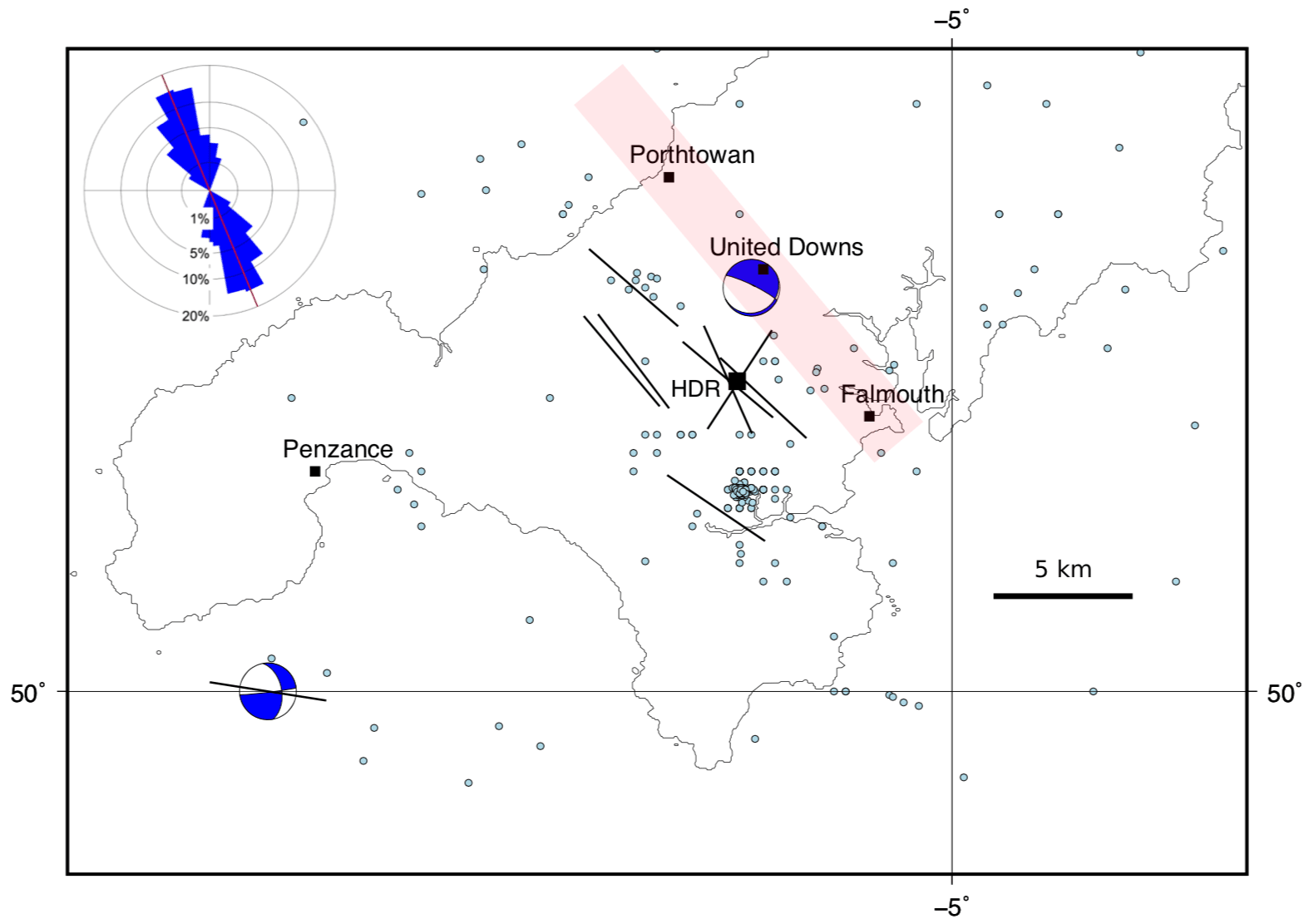
Figure 10Map of southwestern England showing selected population centres, the United Downs deep geothermal pilot project, and the former Hot Dry Rock project (HDR; black squares); epicentres of seismicity (light blue dots; BGS catalogue; Musson, 1996); focal mechanisms (blue and white; Baptie, 2010); and orientations of the maximum horizontal stress (black lines; World Stress Map data; Heidbach et al., 2018). Approximate trend and extent of the Porthtowan Fault Zone shown in pale red. Inset shows an equal-area rose diagram with strikes of fault segments in the Porthtowan Fault Zone measured on BGS Falmouth sheet 352 (N=140; circular mean strike = 158∘; circular standard deviation = 27∘).
The PFZ is poorly exposed inland and runs NNW–SSE from Porthtowan on the northern Cornish coast to Falmouth on the southern coast (Fig. 10; see inset rose diagram for strikes of constituent faults taken from the BGS Falmouth sheet 352). Overall, the fault zone is believed to dip steeply to the east at around 80∘, but note there is considerable variation in strike and dip of individual fault and fracture planes within the fault zone (Fellgett and Haslam, 2021). The azimuth of the maximum horizontal stress is broadly NW–SE, with one exception trending NE–SW.
Detailed geomechanical analyses were performed in the Carnmenellis granite in the 1980s as part of the HDR project, and these provide useful constraints on the variation of stress and fluid pressure with depth (Fig. 12a; Batchelor and Pine, 1986). From these data, a strike-slip regime is most likely with σ1=σHmax and σ2=σV, but note the uncertainties (based on quoted values in Batchelor and Pine, 1986) from around the depth of the injector well at United Downs and deeper; a normal fault regime is also consistent with the data, i.e. σ1=σV and σ2=σHmax. Note that the earlier HDR project did not target a specific fault zone in the granite.
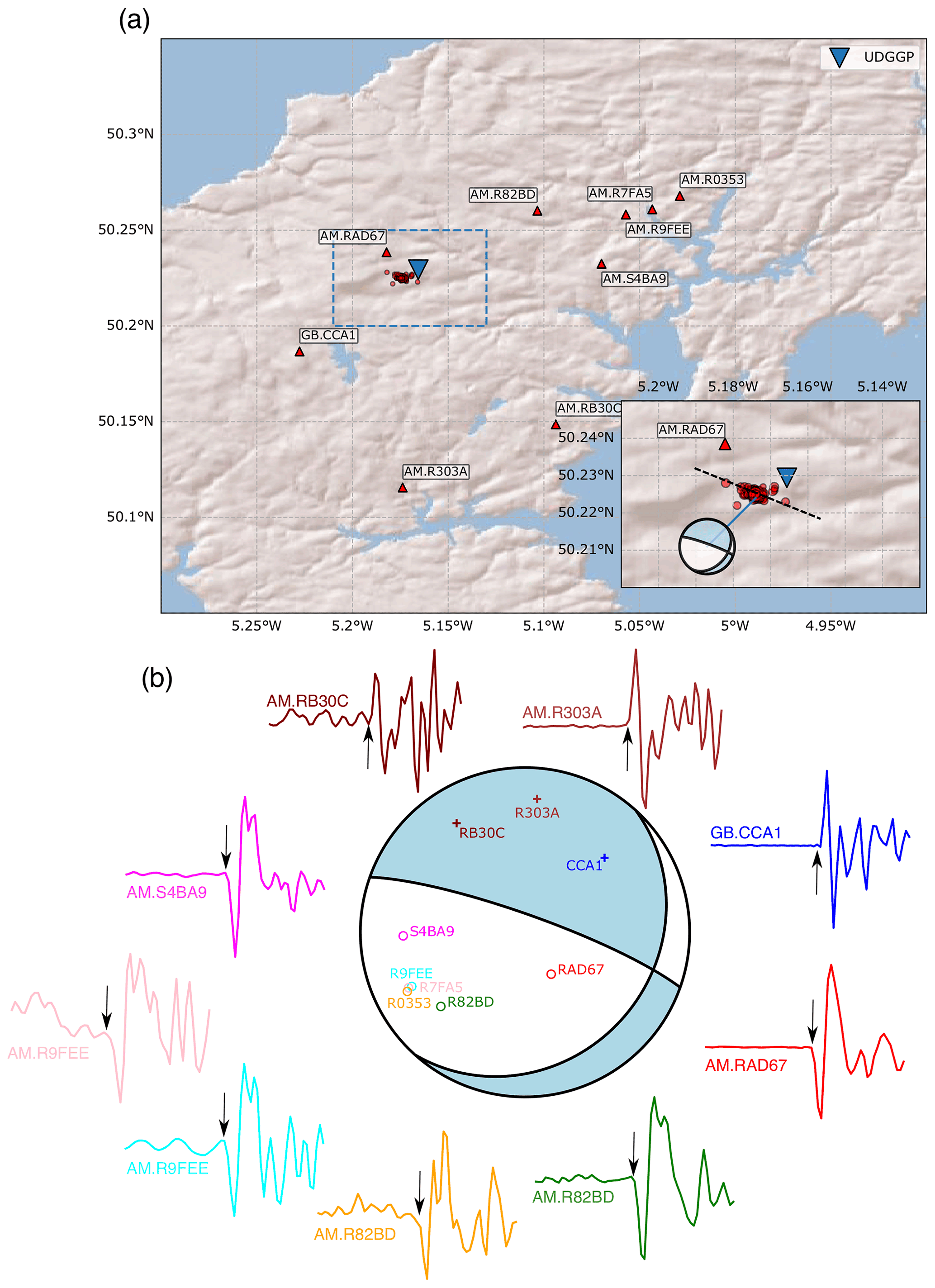
Figure 11(a) Red triangles show Raspberry Shake (network code: AM) and BGS (network code: GB) seismic stations in Cornwall, with station names labelled. Seismicity during geothermal operations is indicated by red circles. The inset shows a close-up of the area demarcated by the dashed blue line in the main map. The dashed black line in the inset shows the broad WNW–ESE alignment in seismicity. (b) Computed focal mechanism for the 30 September 2020, 11:44:01 UTC, ML 1.6 induced earthquake. First motions are plotted on the focal sphere with “+” indicating positive polarity and “o” showing negative polarities. P-wave first motions are plotted starting and ending 0.3 s before and after the picked arrival, respectively, and are coloured in the same way as the points on the focal sphere.
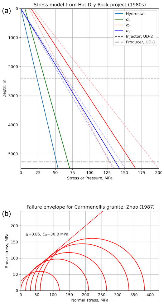
Figure 12Constraints on input variables for the Porthtowan Fault Zone modelling. (a) Stress–depth plot based on data and equations from the Hot Dry Rock project in the Carnmenellis granite (Batchelor and Pine, 1986). Dashed lines show minimum and maximum values for each stress. Also shown are the depths of the two wells in the pilot project at United Downs. (b) Mohr diagram showing data from laboratory mechanical tests of Zhao (1987) for brittle failure of Carnmenellis granite at 200 ∘C. The estimated Mohr–Coulomb failure envelope (dashed red line) is defined by μ=0.85, C0=30 MPa.
The thermo-mechanical properties of the Carnmenellis granite have been studied by Zhao (1987). Figure 12b shows a Mohr diagram of data taken from Table 2.3 of Zhao (1987) for laboratory brittle failure tests conducted at 200 ∘C (the approximate temperature of the injector well at United Downs). From these data, we have estimated a linear Mohr–Coulomb failure envelope defined by a friction coefficient of 0.85 and a cohesive strength of 30 MPa. Cuttings from the boreholes at United Downs have been used to measure friction coefficients of rocks within the PFZ, and values ranging between μ = 0.28–0.6 were recorded (Sanchez-Roa et al., 2020).
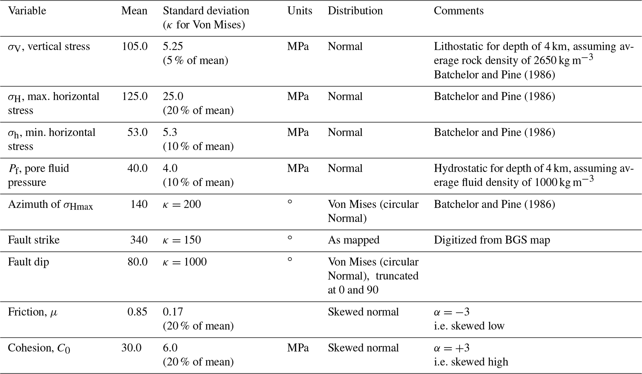
We present model results for fracture susceptibility in the PFZ as the plan at United Downs (and elsewhere in the future) is to inject fluid into the fault zone in order to generate shear-enhanced permeability on pre-existing fractures. Table 3 lists the input variable distributions used in the “base case” model for hydrostatic pore fluid pressure in the fault zone and mechanical properties taken from laboratory tests of intact Carnmenellis granite (Fig. 12b). The modelled depth is chosen as 4 km, in between the depths of the UD-1 and UD-2 wells.
Table 3Distributions of input variables used in the base case model of fracture susceptibility in the Porthtowan Fault Zone.
The results from the Monte Carlo simulation of Sf for the PFZ are shown in Fig. 13. For the base case, with hydrostatic pore fluid pressure and a “strong fault” (mode of μ=0.85, mode of C0=30 MPa), the fault appears unconditionally stable for the modelled in situ stress variations. The CDF shows almost exclusively positive values of Sf up to about 60 MPa. Note that, for the input stress variations listed in Table 3, 22 % of the MC simulations produced an Andersonian normal fault regime (σ1=σV) rather than a strike-slip (σ2=σV) regime.
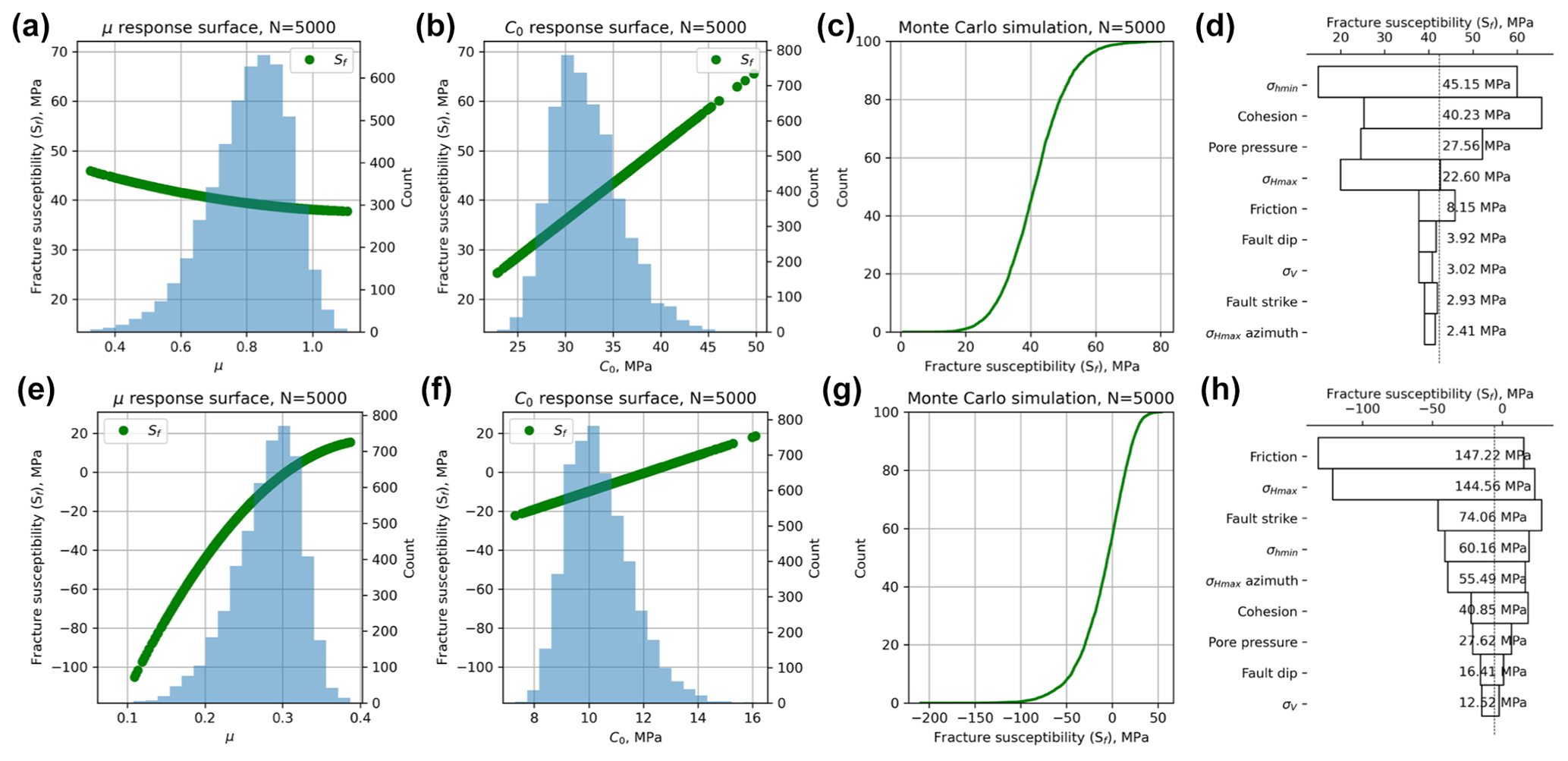
Figure 13Outputs from the Monte Carlo simulation of fracture susceptibility (Sf) in the Porthtowan Fault Zone. (a–d) The response surface for the base case, with friction and cohesion estimated from the laboratory failure tests of Zhao (1987), predicts positive fracture susceptibility, i.e. a stable fault zone. The tornado plot (d) shows that for relatively high values of cohesion (mode of C0=30 MPa in this case), the sensitivity to variations in friction is slight. (e–h) In contrast, the response surface for the “weak fault” case, with reduced values of friction and cohesion (mode of μ=0.3, mode of C0=10 MPa), predicts fault zone instability, i.e. overwhelmingly negative values of Sf. The effect of friction on these predictions is now very strong, as shown in the shape of the response surface for μ (e) and in the ranking within the tornado plot (h).
A total of 232 microseismic events with hypocentre depths of 4–5 km were detected by the BGS during geothermal testing operations in 2021–2022 (http://www.earthquakes.bgs.ac.uk/data/data_archive.html, last access: 23 July 2021). The largest earthquake induced by geothermal operations during this period occurred on 30 September 2020 at 11:44:01 UTC, had a local magnitude of ML 1.6, and was felt by residents in the area. This event was well recorded on a network of single-component Raspberry Shake stations (e.g. Holmgren and Werner, 2021) and a single station of the BGS permanent monitoring network (Fig. 11a). These stations offer excellent azimuthal coverage of the geothermal seismicity, with the closest station lying only 2 km away (AM.RAD67). Since no focal mechanisms have yet been documented for these induced earthquakes, we used recorded P-wave first motions to compute a focal mechanism of the ML 1.6 event using the method of Hardebeck and Shearer (2002). Take-off angles were computed using a 1D seismic velocity model for the Cornwall area (http://earthwise.bgs.ac.uk/index.php/OR/18/015_Table_4:_Depth/crustal_velocity_models_used_in_earthquake_locations, last access: 23 July 2021). The best-fitting focal mechanism (Fig. 11b) indicates either normal faulting on a WNW–ESE steeply dipping plane or strike-slip faulting on a shallowly dipping NE–SW-striking plane. Single-event relocated epicentres reported by the BGS, which use arrivals from a local dedicated microseismic monitoring array, show a NW–SE trend (Fig. 11a), consistent with normal faulting on a steeply eastward-dipping, WNW–ESE-striking plane during this earthquake. Negative P-wave polarities were recorded at AM.RAD67 for all M>0 events, indicating that the same fault plane was likely reactivated during many of the induced events. The inferred fault plane is sub-parallel to the interpreted strike of the Porthtowan Fault Zone that is targeted by the geothermal testing. This observed normal faulting mechanism is consistent with our MC simulations where more than 1 in 5 of the predicted stress states were for normal faulting.
The response surface (green lines on Fig. 13a–b) and the tornado plot of relative sensitivities of the input variables (Fig. 13d) shows a positive dependence of Sf on the cohesion and that variations in friction are relatively unimportant. If we reduce the strength of the modelled fault zone by changing the input distributions of μ and C0 to lower values – but maintain the same shape and skewness – the situation changes. The predicted fracture susceptibility is now much more strongly correlated with variations in friction and less so with variations in cohesion. This can be explained by looking at the underlying formula for Sf (Eq. 3), in particular the second term on the RHS. If C0>τ, then the numerator of this term can be negative, producing a net positive term. However, if C0<τ and μ is small, then this term is larger and negative. The important point is that the probability distribution of Sf (compare Fig. 13c and g) is controlled by the relative magnitudes of μ and C0. In a weak fault zone, with low μ and low C0, the predictions are very sensitive to the value of friction. In a strong fault, the effect of μ is less important. Thus, we need to know more about the relationship between μ and C0 in fault rocks (see Sect. 4).
3.2 South Wales coalfield, UK
Scope exists to extract low-enthalpy geothermal heat from disused coal mines in the UK (Farr et al., 2016) using either open- or closed-loop technology. Possible sites include the South Wales coalfield, where folded and faulted Coal Measures of Westphalian (Upper Carboniferous) age have been mined for centuries up until the 1980s. Initial plans for shallow mine geothermal schemes include passive dewatering, which may not change the loading on faults by much. However, active dewatering schemes can promote ingress of deeper ground water (Farr et al., 2021), and as this fluid flow must be driven by gradients in fluid pressure, this could in turn lead to the instability of faults at greater depth. The models below are for a depth of 2 km.
The locations and orientations of faults have been taken from published BGS maps. We used the BGS Hydrogeology map of South Wales to map the traces of faults in the Coal Measures (Westphalian) and BGS 1 : 50 000 solid geology sheets over the same area to collect data on fault dips (Fig. 14). Faults were traced onto scanned images of the maps in a graphics package (Affinity Designer on an Apple iPad using an Apple Pencil). These fault trace maps were saved in Scalable Vector Graphics (.SVG) format after deleting the original scanned image layer of the geological map. The saved .SVG files were read into FracPaQ (Healy et al., 2017) to quantify their orientation distributions (inset rose plots in Fig. 14a and b). The fault trace maps were then overlain on maps containing historical seismicity and available focal mechanisms (from the public BGS catalogue; Musson, 1996) and the orientations of sHmax taken from the World Stress Map project (Heidbach et al., 2018).
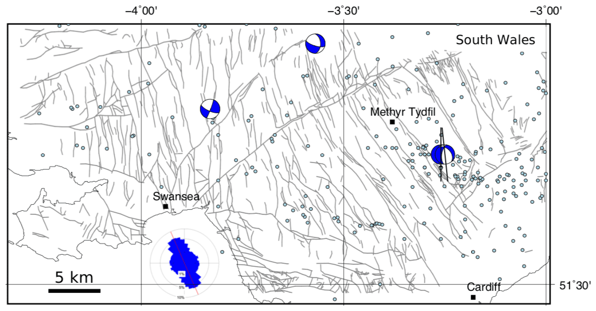
Figure 14Maps of the South Wales coalfield (a suggested site of shallow mine geothermal energy) showing selected population centres (black squares), epicentres of seismicity (light blue dots; BGS catalogue; Musson, 1996), focal mechanisms (blue and white; Baptie, 2010), and orientations of the maximum horizontal stress (black lines; World Stress Map data; Heidbach et al., 2018). Inset equal-area rose diagrams show orientations of mapped faults. Faults in the Coal Measures taken from the BGS Hydrogeological Map of South Wales (1 : 125 000) (n=3408), with a circular mean strike of 156∘ and a circular standard deviation of 65∘.
In the South Wales coalfield, 3408 fault segments were traced, and the dominant trend is clearly NNW–SSE but with important (and long) fault zones running ENE–WSW, such as the Neath and Swansea valley disturbances (Fig. 14). From cross sections, we measured 142 fault dips to help constrain the distribution of friction coefficients in these rocks (Fig. 15b–c; see below), corrected for vertical exaggeration on the section line where necessary. Focal mechanisms in this area (n=4) suggest that NNW–SSE and N–S faults are active in the current stress regime. Historical seismicity is widely, if unevenly, distributed with no obvious direct correlation to the surface mapped fault traces. For example, there are areas of intense surface faulting but no recorded historical seismicity and vice versa, i.e. areas with abundant historical events but few mapped faults.
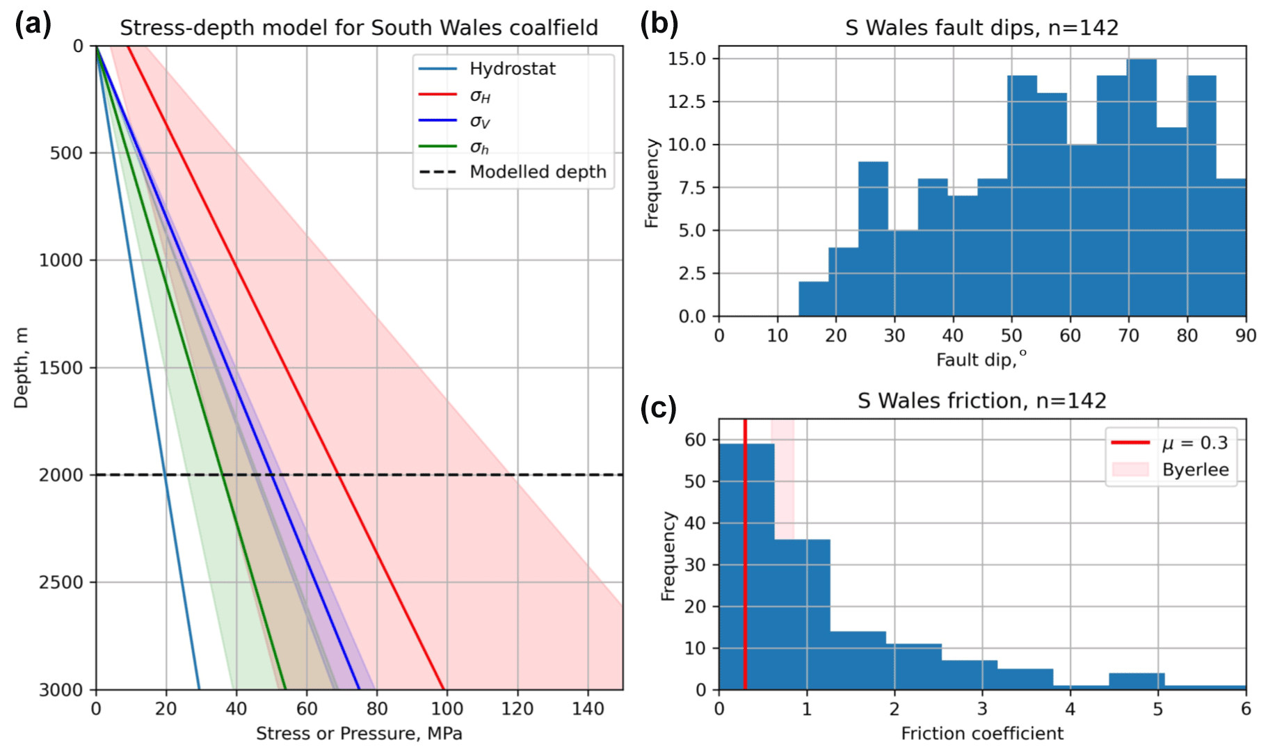
Figure 15Constraints on input variables for the coalfield modelling of slip tendency. (a) Stress–depth plot based on data from onshore UK (after Fellgett et al., 2018). Shaded areas show the extent of uncertainty for each stress. Also shown is the modelled depth of 2 km. (b–c) Histograms of fault dips measured from cross sections on published BGS 1 : 50 000 maps of South Wales and calculated values of friction coefficients derived from these dips assuming Mohr–Coulomb failure. Byerlee friction (μ = 0.6–0.85) is shown as a shaded pink box. Modelled critical values of friction (μ=0.3) are shown by red lines.
There are no published geomechanical analyses for the variation of stress with depth for this area. To constrain the depth dependence of stress, we have used larger-scale syntheses of stress for onshore UK produced by the BGS (e.g. Kingdon et al., 2016; Fellgett et al., 2018). The stress–depth plot in Fig. 15a has been constructed using the data shown in Fellgett et al. (2018) and shows that, in general, a strike-slip fault regime with σ1=σHmax is most likely. However, given the known uncertainties in these data, a normal fault regime (σ1=σV) cannot be ruled out, especially at depth. Note that the stress–depth data shown in Fellgett et al. (2018) and used in Fig. 15a are compiled from different areas and remain untested for the specific area shown in this paper. The azimuth of σHmax is known to vary across the UK, ranging from ∼130 to ∼170 (Baptie, 2010; Becker and Davenport, 2001).
Despite the economic and historical significance of the Coal Measures, there are no published datasets of laboratory-measured friction or cohesion for either intact rocks or their faulted equivalents (although data may exist in proprietary company records). Data for specific units of interest do exist, e.g. for the Oughtibridge Ganister, a seat earth in the Coal Measures (Rutter and Hadizadeh, 1991), and the Pennant Sandstone, a rare marine sandstone unit (Cuss et al., 2003; Hackston and Rutter, 2016), but a systematic analysis of the volumetrically dominant sandstone, siltstone, and mudstone formations is notably absent. Instead, we use the measured dips of faults in the Coal Measures as a proxy for the coefficient of sliding friction, using the relationship
where β is the angle between the fault plane and σ1 at failure (Jaeger et al., 2009; Carvell et al., 2014). Such a calculation assumes Mohr–Coulomb failure and that the current dip of the fault is reasonably close to the dip at failure in the post-Westphalian deformation of the coalfields. For measured fault dips <45∘, we assume that σ1 was horizontal (Andersonian thrust and reverse fault regime) and for fault dips ∘ we assume σ1 was vertical (Andersonian normal fault regime). In practice, some of these faults probably originated as strike-slip faults (i.e. with a sub-vertical dip and σ2 vertical), and some of their dips have almost certainly been modified by compaction since their formation. However, this method of estimating the likely range of friction coefficients from measured dips remains simple to apply and useful to the first order, in the absence of better data. From the dip data, the calculated friction coefficients vary between 0.0 and 6.0 for South Wales (Fig. 15b, c).
Based on the values of sliding friction calculated from measured fault dips across the coalfield a threshold stability value of μ=0.3 is taken as a reasonable lower bound for faulted rock. This is the value used to compare with predicted slip tendencies calculated for each fault. For Ts>0.3, the fault is deemed unstable, and for it is stable.
Predictions of conditional probability for fault slip have been calculated for all faults in the coalfield using slip tendency as the chosen measure: in the absence of detailed pore fluid pressure constraints or estimates of cohesive strength, it is hard to justify modelling the fracture susceptibility. Slip tendency provides a first-order estimate of fault stability. A quadratic response surface was constructed for the coalfield using the full range of measured fault strikes and dips, and the input variable distributions listed in Table 4 and constrained by the data in Fig. 15. Monte Carlo simulations (NMC=5000) were run for each mapped fault segment with the other input variables drawn from their respective distributions.
Table 4Distributions of input variables used to model slip tendency in the coalfields of South Wales.

Output CDFs for all faults are shown in Fig. 16. For South Wales (N=3408 faults), approximately 46 % of faults are predicted to have a 1 in 3 chance of being unstable (i.e. Ts>0.3, shown in red), and 42 % of faults are predicted to have a 1 in 100 chance of being unstable (shown in amber).
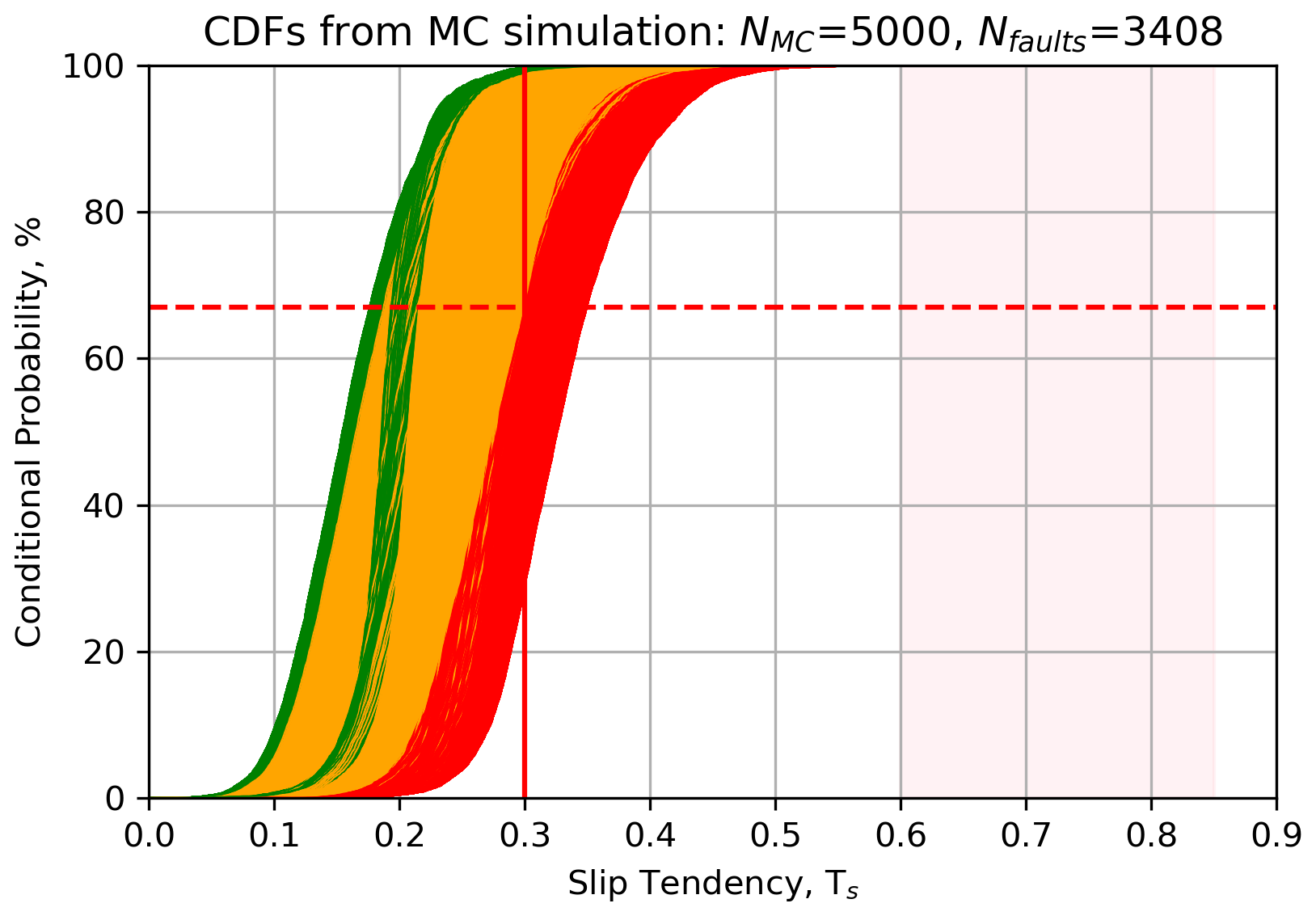
Figure 16Output from the Monte Carlo modelling of slip tendency (Ts) in South Wales coalfield, UK. For slip tendency, more stable faults skew towards the left (low Ts), less stable faults skew to the right (high Ts). CDFs of predicted slip tendency for each mapped fault in South Wales. Colour coding of CDFs is as follows: red shows >33 % chance of exceeding threshold friction (μ=0.3, vertical red line), amber shows between >1 % and <33 % chance, and green shows <1 % chance. The range of Byerlee friction is shown by pink shading.
The results from the RSM–MC modelling shown in the CDF are replicated in map view in Fig. 17. Each fault segment is colour coded using the same heuristic applied in the CDF: red faults have a conditional probability of at least 33% of their slip tendency exceeding the chosen threshold value of fault rock friction (μ=0.3), amber (orange) faults have a 1 %–33 % chance, and green faults have a less than 1 % chance of being unstable.
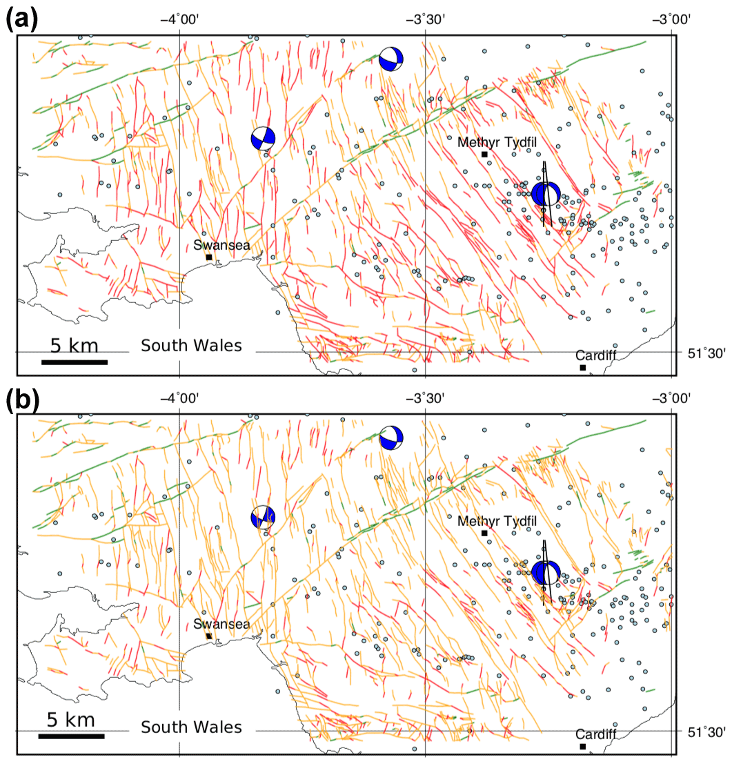
Figure 17Output from the Monte Carlo modelling of slip tendency (Ts) in South Wales coalfield. (a) Colour-coded fault map showing conditional probability of slip for each mapped fault. This map shows the unweighted values, as shown on the CDFs in Fig. 14a. (b) Colour-coded fault map showing conditional weighted probability of slip for each mapped fault. The weighted probability is calculated by multiplying the probability from the CDF in Fig. 14a by the normalized fault smoothness, ranging from 1.0 for a perfectly straight (i.e. smooth) fault and tending to 0.0 for a rough fault. Colour coding of CDFs is as follows: red shows >33 % chance of exceeding threshold friction (μ=0.3), amber shows between >1 % and <33 % chance, and green shows <1 % chance.
For South Wales, the general pattern of the predictions is consistent with the recorded focal mechanisms (Fig. 17a). The most likely fault segments to slip (coloured red) are those oriented either NNW–SSE or N–S, corresponding with one of the nodal planes in each of the focal mechanisms. Faults trending ENE–WSW, such as the Neath disturbance, are predicted to have low probability of slip in the modelled stress regime (green). Note that the Swansea Valley disturbance trends ENE–WSW as a fault zone, but the constituent fault segments are variously oriented, including elements that trend NE–SW, and these are marked in red (high probability of slip). Blenkinsop et al. (1986) noted that this fault zone may in fact have a shallow dip at depth, which is not covered by the dip distribution used in our modelling, and thus further work is required here. The location with the most recorded events lies to the SE of Merthyr Tydfil, and this corresponds to an area with many mapped faults trending NW–SE marked with a high probability of slip, and consistent with two of the focal mechanisms.
4.1 Stress, pressure, and temperature
The simulations described in this paper all critically depend on our knowledge of the in situ stress tensor. We can constrain some of the components of this tensor better than others. The vertical stress (σV) is usually the best constrained, a reflection of its derivation from the borehole density logs sampled at sub-metre resolution. Our estimates of the horizontal stresses, σHmax and σhmin, remain poorly constrained. Even in cases with relatively good data, e.g. from borehole leak-off tests (LOTs) and formation integrity tests (FITs), the “data density” for these stress components is generally sparse (compared to σV), and we are stuck with significant uncertainties. These uncertainties are important, as shown by this study and previous work (e.g. Chiaramonte et al., 2008; Walsh and Zoback, 2016). The fundamental dependence of shear failure on differential stress inherent in the Mohr–Coulomb failure criterion is reflected in the high ranking of stress tensor components in the tornado plots shown in this study. In addition, larger uncertainties in stress components mean that the Andersonian regime may flip from the default “average” assumption to another orientation: for example, an apparently strike-slip regime may in fact include a significant proportion of normal fault possibilities (>20 % in the case of the Porthtowan Fault Zone shown here). One way to improve our knowledge of the stress tensor and especially the azimuth of σHmax would be to exploit richer catalogues of seismicity to produce more focal mechanisms for natural or induced events. Most countries would benefit from better, i.e. more widespread and higher resolution, continuous seismic monitoring. While this may be expensive with top-of-the-range broadband equipment, citizen science devices, such as the Raspberry Shake, offer a low-cost and viable alternative (Cochran, 2018; Anthony et al., 2019; Hicks et al., 2019; Holmgren and Werner, 2021). Our study shows how Raspberry Shake data are effective for computing focal mechanisms. Analysis of more events would allow stress inversions to be performed on the data measured by these devices, especially when they are combined in ad hoc arrays to improve signal-to-noise ratios.
Pore fluid pressures at depth are also poorly known, even for a country like the UK with a long tradition of geological (and geophysical) science and a rich history of mining and drilling into the crust. Most importantly, our knowledge of measured in situ pore fluid pressures in and around fault zones is generally poor. Theoretical predictions and model simulations abound, but direct measurements of this key parameter are almost non-existent. We need to know the actual limits of pore fluid pressures in fault zones and their likely spatial and temporal variation over a fault plane throughout the seismic cycle. The situation is complicated by the finer-scale structure of fault zones. Fault zones in low-porosity and/or crystalline rocks (such as granite) can be divided into one or more narrow cores defined by fine-grained fault rocks (gouges, cataclasites) surrounded by wider damage zones of more or less fractured rock. Permeability may be low in and across the core(s) and higher in the damage zones (Caine et al., 1996; Faulkner et al., 2010). In high-porosity and/or granular rocks (such as sandstone), fault zones may be simpler, with fine-grained fault rocks along narrow fault planes forming an effective fluid seal (Wibberley et al., 2008) These differences in the physical characteristics of the fault zones have consequences for the distribution of dynamic pore fluid pressures, which remain poorly known in detail.
The work described in this paper has ignored the effects of temperature. However, thermoelastic stress may be more important than poroelastic stress by a factor of 10 (Jacquey et al., 2015). In short, colder injected water may increase the chance of slip on a given fault. In the UK, our knowledge of the subsurface temperature field is increasing (Beamish and Busby, 2016; Farr et al., 2021), but we need more data, especially from faulted rocks.
4.2 Faults
An implicit assumption in all of the modelling performed in this paper (and many others) is that we know something about the fault which may slip: i.e. we can only quantify risk on known faults. There will, in general, be many more unmapped faults in the subsurface, and these may be the ones most likely to slip due to a change in loading (of either in situ stress or fluid pressure). This is apparent in the maps for the coalfields shown in this paper in terms of the relative lack of correspondence between the surface mapped fault traces and the locations of recorded earthquakes. Some, but not all, of this “mismatch” could be explained by the dip of the faults measured at the surface. Moreover, there are areas of apparently intense surface faulting and no recorded seismicity and vice versa (recorded seismicity but no mapped surface faults). Some advances could be made to address this problem with the recognition that each recorded seismic event documents a fault plane, assuming that a double couple focal mechanism implies fault slip rather than dilation from dyke emplacement or other mechanisms. Therefore, the 3D position of each focal mechanism points to at least part of a subsurface fault. The challenge then lies in mapping these seismic event fault planes into a viable fault network. Better data (i.e. higher spatial resolution and extending to smaller event magnitudes) from more dense arrays of seismometers would help with this task, as for the refinement of stress estimates noted above.
4.3 Rock properties
The importance of good data on rock properties has been emphasized above in the worked example for fracture susceptibility and in the case study for the Porthtowan Fault Zone. In general, we need more and better data on coefficients of friction and cohesive strength, especially for the target formations of decarbonization operations. Moreover, we need data for the intact and faulted rocks. We also need better constrained correlations among rock properties. A widely used method in oil and gas is to derive estimates of friction coefficient and unconfined compressive strength (UCS) from wireline log datasets measuring porosity, slowness (velocity), or elasticity, e.g. Chang et al. (2006). However, as noted by these authors, the correlations are strictly valid only for the specific formations tested in the laboratory, and even then the uncertainties remain large. A further issue is the tendency to average wireline log-derived estimates over a depth interval, when for most sections of crust this is the direction in which rock properties are expected to vary most rapidly. The Porthtowan Fault Zone example above highlighted another issue: the relative impact of cohesion and friction on the predicted stability depends on the magnitude of the cohesion in relation to the shear stress on the fault. For low cohesion values, the constraints on friction become much more important. We need systematic investigations of frictional behaviour at low cohesive strength and detailed systematic correlations among rock properties, especially for faulted crystalline basement rocks.
Collecting more laboratory data is no panacea, evidenced by the well-aired concerns over how we upscale rock properties and behaviours from millimetre- and centimetre-sized samples to whole fault zones. However, calibrations and correlations from careful, systematic laboratory data remain the cornerstone of estimating the key in situ values. An interesting new focus would be to explore the nature of the skewness in mechanical property datasets: why should friction coefficients skew low and cohesive strength skew high?
The utility of the Mohr–Coulomb criterion used in this paper is largely down to its mathematical simplicity, i.e. linearity and only two parameters (friction and cohesion). Other criteria are perfectly viable and could easily be added to the pfs Python code, but some other failure criteria lack a clear mapping between their parameters and the mechanics of sliding on rock surfaces.
4.4 Applicability of Ts, Td, and Sf for quantifying risk
A valid question is to ask whether any of these widely used measures of fault stability are, in fact, useful in practical terms at the scale of faults on maps. All three measures focus on the simplified mechanics of slip on a specific fault plane, with a fixed orientation, and with specific rock properties. However, seismic hazard is not isolated at the level of single fault planes. Faults occur in patterns or networks that are more or less linked together. Geometrical factors may be more important than the specifics of either the in situ stress or the rock properties at the scale of observation. The observational record shows that bigger fault zones are the sites of bigger earthquakes, and they are also the locus of most displacement in a given network. Conversely, smaller faults host smaller seismic events and accrue less overall displacement (Walsh et al., 2001). To begin to address this issue, we can weight the conditional probabilities of slip for a specific fault segment by a dimensionless normalized factor derived from the total length of the fault: e.g. , where Ls is fault segment length and Lt is fault trace length. An alternative but related idea is that of the relationship between fault smoothness (or inversely, roughness) and fault maturity and therefore seismic hazard (Wesnousky, 1988; Wells and Coppersmith, 1994; Leonard, 2010). The most seismically active faults are not only (or necessarily) the largest ones in their network but tend to be the smoothest or most connected, reflecting the coalescence of fault segments through time and the removal of asperities through repeated slip events (Stirling et al., 1996). Therefore, we can weight the conditional probabilities of slip by a dimensionless factor of smoothness: , where Lstraight is the straight line length between fault end points, which is 1.0 for a perfectly smooth fault with all segments parallel and connected and tends to 0.0 for rough, complex fault traces. An example of the effect of these smoothness weightings applied to the conditional probabilities is shown in Fig. 17b for the South Wales coalfield faults. The net effect is to reduce the number of most risky faults (shown in red) by about half. These approaches are the subject of further work and testing.
In this paper, we have described and explained the response surface methodology and shown how it can be combined with a Monte Carlo approach to generate probabilistic estimates of fault stability using published measures of slip tendency, dilation tendency, and fracture susceptibility. Simulations show that a quadratic response surface always generates a better fit to the input variables in comparison to a linear surface, at the cost of larger matrices (more computer memory) and longer run times. Worked examples to calculate Ts and Sf with synthetic input distributions show how the quadratic response surfaces vary for each input parameter. For slip and dilation tendency, the primary dependence is (as expected) on the maximum differential stress, and therefore the maximum and minimum principal stresses of the in situ stress tensor, with a lesser dependence on the fault orientation. For fracture susceptibility, the situation is more complex: if cohesion is relatively high, Sf is mainly dependent on the in situ stresses and cohesion. But if cohesion is low – quite likely in fault zones – then the dependence of Sf on friction is much more significant. This is a key finding: the relative sensitivity of the input variables on the response surface varies with the absolute value of the variables.
Sensitivity tests were used to assess how the shapes of different input distributions affect the predictions of fault stability. Varying the spread of symmetric (normal, Gaussian) distributions of input variables has a significant effect on the predictions, and this mirrors the reality of uncertainties in, for example, the principal stresses in a standard geomechanical analysis. As noted above, the vertical stress is often well constrained and has a lower relative standard deviation (say, 5 % of the mean) than either the maximum or minimum horizontal stresses (typically 15 %–20 % of their mean value). The shape and spread of skewed (asymmetric) distributions of rock properties (friction and cohesion) is also important. The direction of skewness is described by the sign of the parameter α for the skewed normal distributions used in this paper to model variations in rock properties. Friction is modelled with a negative skewness towards lower values, whereas cohesion is modelled with positive skewness towards higher values, but systematic laboratory data are needed to verify these assumptions. This will require a statistically significant number of repeat tests for each property on quasi-identical samples of the same rock.
Case studies of two different locations demonstrated how a probabilistic approach can provide a useful assessment of fault stability, including which of the input variables are the most important for a given combination of in situ stress, fault plane orientations, and rock properties. This then enables greater focus on improving the estimates of the key variables, and the relationships between them. For the Porthtowan Fault Zone in Cornwall, the modelling in this paper shows that we need more data for, and a better understanding of the relationship between, coefficients of friction and cohesive strength, especially at low values of friction (i.e. less than the Byerlee range of 0.6–0.85) to be expected in fault zones. For the South Wales coalfield, model outputs show how predictions of fault stability can be weighted by a simple index of fault smoothness to begin to allow for the effects of geometrical weakening within the fault system as whole, rather than focusing on each individual fault plane taken in isolation.
It is obvious that uncertainty in the input parameters must translate into uncertainty in the output predictions. By combining a response surface methodology with a Monte Carlo approach to the quantification of fault stability, we can explore, understand, and quantify how differing degrees of uncertainty among the input parameters feed through to uncertainty in the predicted stability measure. Response surfaces and tornado plots can help to identify which parameters are the most important in a particular analysis. Given our current state of knowledge of stress, fault orientations, and fault rock properties, probabilistic estimates and iterative modelling are useful approaches to begin to de-risk the energy transition. Free, open-source software to perform these analyses, such as the Python package pfs, can help to encourage their wider adoption and further refinement (“given enough eyeballs, all bugs are shallow”; Raymond, 2001). The deployment of abundant and relatively low-cost citizen science seismometers (e.g. Raspberry Shakes) could synergize two critical issues: the wider involvement of the public into open science debates about risk and the simultaneous collection of better data to constrain the local stress field. The energy transition and decarbonization are urgent and essential tasks: we will only be successful if we manage to balance public perceptions of risk with the technical challenges inherent to the exploitation of faulted rock.

Figure A1Histograms of input variables used to calculate dilation tendency (Td) for the synthetic distributions shown in Table 2.
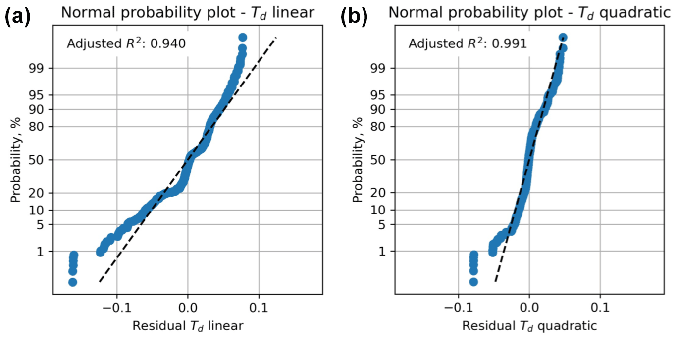
Figure A2Residual plots for linear and quadratic response surfaces for dilation tendency (Td) using synthetic data. The quadratic fit has a higher value of the adjusted R2 parameter and is therefore deemed better in this case.
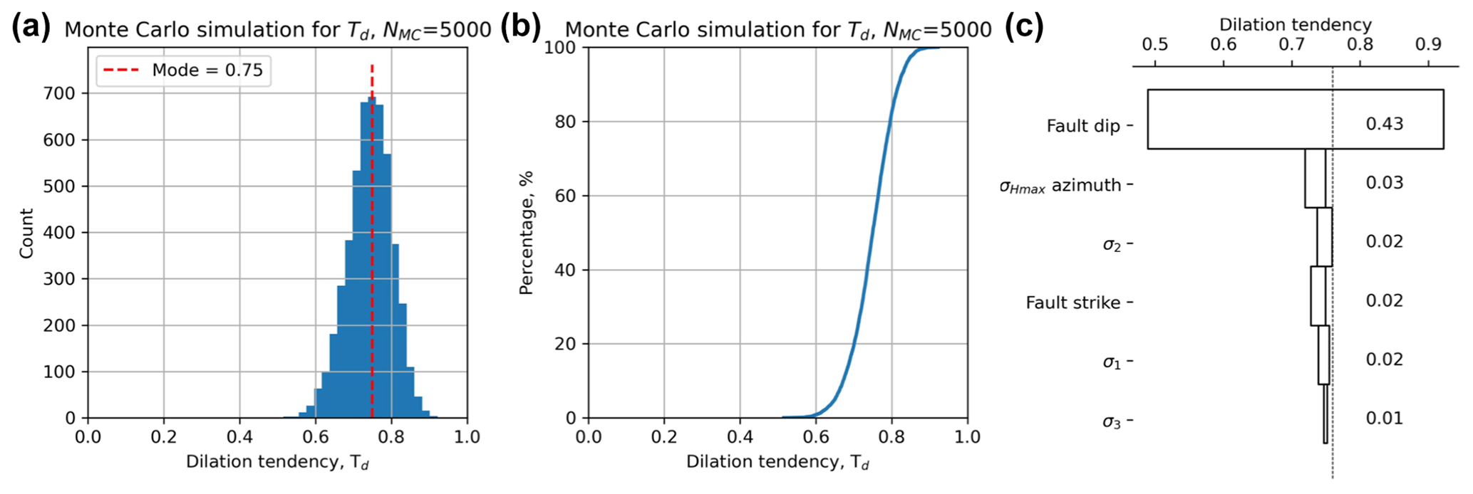
Figure A3Output from Monte Carlo simulation (NMC=5000) of dilation tendency calculated using a quadratic response surface from synthetic input data. (a) Histogram of calculated dilation tendency values, in this case showing a quasi-normal distribution with a mode of ∼ 0.75. (b) Cumulative distribution function (CDF) of calculated dilation tendency values, showing the range in values from ∼ 0.5 to ∼ 0.9.
The code used in this study is available at https://github.com/DaveHealy-github/pfs, last access: 6 January 2022 (https://zenodo.org/badge/latestdoi/377846715, Healy, 2021).
No data sets were used in this article.
DH originated the study, wrote the code, and ran the models. SPH contributed seismology data and expertise and to the writing of the text.
At least one of the (co-)authors is a member of the editorial board of Solid Earth. The peer-review process was guided by an independent editor, and the authors also have no other competing interests to declare.
Publisher's note: Copernicus Publications remains neutral with regard to jurisdictional claims in published maps and institutional affiliations.
David Healy first presented the core ideas in this paper at the Tectonic Studies Group AGM in Cardiff in 2014 and enjoyed discussions there with Jonathan Turner (RWM Ltd). Thanks to former PhD student Sarah Weihmann (now at BGR) and co-supervisor Frauke Schaeffer (Wintershall DEA) for discussions about using oil industry wireline log data for quantifying geomechanical models. Thanks to Tom Blenkinsop (Cardiff) for the idea of using fault dips to estimate friction coefficients. Generic Mapping Tools (GMT) (Wessel et al., 2013) was used for the maps. SciPy (Virtanen et al., 2020), Numpy (Harris et al., 2020), and Matplotlib (Hunter, 2007) were used for the Python pfs code, and Allmendinger et al. (2011) was used for various geomechanical and geometrical algorithms. We thank the reviewers for their comments that improved the manuscript. David Healy acknowledges NERC funding from grant NE/T007826/1.
This research has been supported by the Natural Environment Research Council (grant no. NE/T007826/1).
This paper was edited by Federico Rossetti and reviewed by Jonathan Turner and one anonymous referee.
Alcalde, J., Bond, C. E., Johnson, G., Ellis, J. F., and Butler, R. W.: Impact of seismic image quality on fault interpretation uncertainty, GSA Today, https://doi.org/10.1130/GSATG282A.1, 2017.
Allmendinger, R. W., Cardozo, N., and Fisher, D. M.: Structural geology algorithms: Vectors and tensorsm Cambridge University Press, ISBN 978-1-10-740138-9, 2011.
Anthony, R. E., Ringler, A. T., Wilson, D. C., and Wolin, E.: Do low-cost seismographs perform well enough for your network? An overview of laboratory tests and field observations of the OSOP Raspberry Shake 4D, Seismol. Res. Lett., 90, 219–228, 2019.
Ayash, S. C., Dobroskok, A. A., Sorensen, J. A., Wolfe, S. L., Steadman, E. N., and Harju, J. A.: Probabilistic approach to evaluating seismicity in CO2 storage risk assessment, Enrgy. Proced., 1, 2487–2494, 2009.
Baptie, B.: Seismogenesis and state of stress in the UK, Tectonophysics, 482, 150–159, 2010.
Barcelona, H., Yagupsky, D., Vigide, N., and Senger, M.: Structural model and slip-dilation tendency analysis at the Copahue geothermal system: inferences on the reservoir geometry, J. Volcanol. Geoth. Res., 375, 18–31, 2019.
Batchelor, A. S. and Pine, R. J.: The results of in situ stress determinations by seven methods to depths of 2500 m in the Carnmenellis granite, in: ISRM International Symposium, OnePetro, August 1986, Stockholm, Sweden, 1986.
Beamish, D. and Busby, J.: The Cornubian geothermal province: heat production and flow in SW England: estimates from boreholes and airborne gamma-ray measurements, Geothermal Energy, 4, 1–25, 2016.
Becker, A. and Davenport, C. A.: Contemporary in situ stress determinations at three sites in Scotland and northern England, J. Struct. Geol., 23, 407–419, 2001.
Blenkinsop, T. G., Long, R. E., Kusznir, N. J., and Smith, M. J.: Seismicity and tectonics in Wales, J. Geol. Soc., 143, 327–334, 1986.
Bond, C. E.: Uncertainty in structural interpretation: Lessons to be learnt, J. Struct. Geol., 74, 185–200, 2015.
Box, G. E. and Wilson, K. B.: On the Experimental Attainment of Optimum Conditions, J. R. Stat. Soc. B, 13, 1–45, 1951.
Caine, J. S., Evans, J. P., and Forster, C. B.: Fault zone architecture and permeability structure, Geology, 24, 1025–1028, 1996.
Carvell, J., Blenkinsop, T., Clarke, G., and Tonelli, M.: Scaling, kinematics and evolution of a polymodal fault system: Hail Creek Mine, NE Australia, Tectonophysics, 632, 138–150, 2014.
CCC (UK Committee on Climate Change): Net Zero–Technical Report, available at: https://www.theccc.org.uk/wp-content/uploads/2019/05/Net-Zero-Technical-report-CCC.pdf (last access: 6 January 2022), 2019.
Chang, C., Zoback, M. D., and Khaksar, A.: Empirical relations between rock strength and physical properties in sedimentary rocks, J. Petrol. Sci. Eng., 51, 223–237, 2006.
Chiaramonte, L., Zoback, M. D., Friedmann, J., and Stamp, V.: Seal integrity and feasibility of CO2 sequestration in the Teapot Dome EOR pilot: geomechanical site characterization, Environ. Geol., 54, 1667–1675, 2008.
Clarke, H., Verdon, J. P., Kettlety, T., Baird, A. F., and Kendall, J. M.: Real-time imaging, forecasting, and management of human-induced seismicity at Preston New Road, Lancashire, England, Seismol. Res. Lett., 90, 1902–1915, 2019.
Cochran, E. S.: To catch a quake, Nat. Commun., 9, 1–4, 2018.
Cuss, R. J., Rutter, E. H., and Holloway, R. F.: The application of critical state soil mechanics to the mechanical behaviour of porous sandstones, Int. J. Rock Mech. Min., 40, 847–862, 2003.
Das, D. and Mallik, J.: Koyna earthquakes: a review of the mechanisms of reservoir-triggered seismicity and slip tendency analysis of subsurface faults, Acta Geophys., 68, 1097–1112, 2020.
Ellsworth, D., Spiers, C. J., and Niemeijer, A. R.: Understanding induced seismicity, Science, 354, 1380–1381, 2016.
Farr, G., Sadasivam, S., Watson, I. A., Thomas, H. R., and Tucker, D.: Low enthalpy heat recovery potential from coal mine discharges in the South Wales Coalfield, Int. J. Coal Geol., 164, 92–103, 2016.
Farr, G., Busby, J., Wyatt, L., Crooks, J., Schofield, D. I., and Holden, A.: The temperature of Britain's coalfieldsm Q. J. Eng. Geol. Hydroge., 54, https://doi.org/10.1144/qjegh2020-109, 2021.
Faulkner, D. R., Jackson, C. A. L., Lunn, R. J., Schlische, R. W., Shipton, Z. K., Wibberley, C. A. J., and Withjack, M. O.: A review of recent developments concerning the structure, mechanics and fluid flow properties of fault zones, J. Struct. Geol., 32, 1557–1575, 2010.
Fellgett, M. W. and Haslam, R.: Fractures in Granite: Results from United Downs Deep Geothermal well UD-1, EGU General Assembly 2021, online, 19–30 April 2021, EGU21-5593, https://doi.org/10.5194/egusphere-egu21-5593, 2021.
Fellgett, M. W., Kingdon, A., Williams, J. D., and Gent, C. M.: Stress magnitudes across UK regions: New analysis and legacy data across potentially prospective unconventional resource areas, Mar. Petrol. Geol., 97, 24–31, 2018.
Ferrill, D. A., Winterle, J., Wittmeyer, G., Sims, D., Colton, S., Armstrong, A., and Morris, A. P.: Stressed rock strains groundwater at Yucca Mountain, Nevada, GSA Today, 9, 1–8, 1999.
Goebel, T. H. W., Rosson, Z., Brodsky, E. E., and Walter, J. I.: Aftershock deficiency of induced earthquake sequences during rapid mitigation efforts in Oklahoma, Earth Planet. Sc. Lett., 522, 135–143, 2019.
Green, A. S. P., Baria, R., Madge, A., and Jones, R.: Fault-plane analysis of microseismicity induced by fluid injections into granite, Geol. Soc. Eng. Geol. Sp., 5, 415–422, 1988.
Hackston, A. and Rutter, E.: The Mohr–Coulomb criterion for intact rock strength and friction – a re-evaluation and consideration of failure under polyaxial stresses, Solid Earth, 7, 493–508, https://doi.org/10.5194/se-7-493-2016, 2016.
Hardebeck, J. L. and Shearer, P. M.: A new method for determining first-motion focal mechanisms, B. Seismol. Soc. Am., 92, 2264–2276, 2002.
Harris, C. R., Millman, K. J., van der Walt, S. J., Gommers, R., Virtanen, P., Cournapeau, D., Wieser, E., Taylor, J., Berg, S., Smith, N. J., and Kern, R.: Array programming with NumPy, Nature, 585, 357–362, 2020.
Healy, D.: Probability of fault slip, Zenodo [data set], available at: https://zenodo.org/badge/latestdoi/377846715, last access: 6 January 2022.
Healy, D., Rizzo, R. E., Cornwell, D. G., Farrell, N. J., Watkins, H., Timms, N. E., Gomez-Rivas, E., and Smith, M.: FracPaQ: A MATLAB™ toolbox for the quantification of fracture patterns, J. Struct. Geol., 95, 1–16, 2017.
Heidbach, O., Rajabi, M., Cui, X., Fuchs, K., Müller, B., Reinecker, J., Reiter, K., Tingay, M., Wenzel, F., Xie, F., and Ziegler, M. O.: The World Stress Map database release 2016: Crustal stress pattern across scales, Tectonophysics, 744, 484–498, 2018.
Hennings, P. H., Lund Snee, J. E., Osmond, J. L., DeShon, H. R., Dommisse, R., Horne, E., Lemons, C., and Zoback, M. D.: Injection-induced seismicity and fault-slip potential in the Fort Worth Basin, Texas, B. Seismol. Soc. Am., 109, 1615–1634, 2019.
Hicks, S., Goes, S., Whittaker, A. C., and Stafford, P. J. Multivariate statistical appraisal of regional susceptibility to induced seismicity: application to the Permian Basin, SW United States, J. Geophys. Res.-Sol. Ea., 126, e2021JB022768, https://doi.org/10.1029/2021jb022768, 2021.
Hicks, S. P., Verdon, J., Baptie, B., Luckett, R., Mildon, Z. K., and Gernon, T.: A shallow earthquake swarm close to hydrocarbon activities: Discriminating between natural and induced causes for the 2018–2019 Surrey, United Kingdom, earthquake sequence, Seismol. Res. Lett., 90, 2095–2110, 2019.
Hincks, T., Aspinall, W., Cooke, R., and Gernon, T. Oklahoma's induced seismicity strongly linked to wastewater injection depth, Science, 359, 1251–1255, 2018.
Holmgren, J. M. and Werner, M. J.: Raspberry Shake Instruments Provide Initial Ground-Motion Assessment of the Induced Seismicity at the United Downs Deep Geothermal Power Project in Cornwall, United Kingdom, Seismic Record, 1, 27–34, 2021.
Hunter, J. D.: Matplotlib: A 2D graphics environment, Comput. Sci. Eng., 9, 90–95, 2007.
IPCC: Global warming of 1.5 ∘C. An IPCC Special Report on the impacts of global warming of 1.5 ∘C above pre-industrial levels and related global greenhouse gas emission pathways, in the context of strengthening the global response to the threat of climate change, sustainable development, and efforts to eradicate poverty, edited by: Masson-Delmotte, V., Zhai, P., Pörtner, H. O., Roberts, D., Skea, J., Shukla, P. R., Pirani, A., Moufouma-Okia, W., Péan, C., Pidcock, R., and Connors, S., 1, 1–9, 2018.
Jaeger, J. C., Cook, N. G., and Zimmerman, R.: Fundamentals of rock mechanics, John Wiley and Sons, ISBN 978-0-632-05759-7, 2009.
Jacquey, A. B., Cacace, M., Blöcher, G., and Scheck-Wenderoth, M.: Numerical investigation of thermoelastic effects on fault slip tendency during injection and production of geothermal fluids, Enrgy. Proced., 76, 311–320, 2015.
Kingdon, A., Fellgett, M. W., and Williams, J. D.: Use of borehole imaging to improve understanding of the in-situ stress orientation of Central and Northern England and its implications for unconventional hydrocarbon resources, Mar. Petrol. Geol., 73, 1–20, 2016.
Ledingham, P., Cotton, L., and Law, R.: The united downs deep geothermal power project, in: Proceedings of the 44th Workshop on Geothermal Reservoir Engineering, Stanford University, Stanford, CA, USA, 11–13, 2019.
Leonard, M.: Earthquake fault scaling: Self-consistent relating of rupture length, width, average displacement, and moment release, B. Seismol. Soc. Am., 100, 1971–1988, 2010.
Li, X., Main, I., and Jupe, A.: Induced seismicity at the UK “hot dry rock” test site for geothermal energy production, Geophys. J. Int., 214, 331–344, 2018.
Lisle, R. J. and Srivastava, D. C.: Test of the frictional reactivation theory for faults and validity of fault-slip analysis, Geology, 32, 569–572, 2004.
McLennan, D., Noble, S., Noble, M., Plunkett, E., Wright, G., and Gutacker, N.: The English indices of deprivation 2019: Technical report, available at: https://assets.publishing.service.gov.uk/government/uploads/system/uploads/attachment_data/file/833951/IoD2019_Technical_Report.pdf (last access: 6 January 2022), 2019.
Miocic, J. M., Johnson, G., and Bond, C. E.: Uncertainty in fault seal parameters: implications for CO2 column height retention and storage capacity in geological CO2 storage projects, Solid Earth, 10, 951–967, https://doi.org/10.5194/se-10-951-2019, 2019.
Moeck, I., Kwiatek, G., and Zimmermann, G.: Slip tendency analysis, fault reactivation potential and induced seismicity in a deep geothermal reservoir, J. Struct. Geol., 31, 1174–1182, 2009.
Moos, D., Peska, P., Finkbeiner, T., and Zoback, M.: Comprehensive wellbore stability analysis utilizing quantitative risk assessment, J. Petrol. Sci. Eng., 38, 97–109, 2003.
Morris, A., Ferrill, D. A., and Henderson, D. B.: Slip-tendency analysis and fault reactivation, Geology, 24, 275–278, 1996.
Musson, R. M.: The seismicity of the British Isles, Ann. Geophys., 39, https://doi.org/10.4401/ag-3982, 1996.
Myers, R. H., Montgomery, D. C., and Anderson-Cook, C. M.: Response surface methodology: process and product optimization using designed experiments, John Wiley and Sons, ISBN 978-1-118-91601-8, 2016.
Nolan, L.: The Welsh Index of Multiple Deprivation, in: Presentation for the GSS Methodology Conference, Vol. 6, available at: https://your-biz.org/wp-content/uploads/2014/11/welshindexofmultipledeprivatio_tcm77-281304.pdf (last access: 6 January 2022), 2016.
Pine, R. J. and Batchelor, A. S.: Downward migration of shearing in jointed rock during hydraulic injections, International Journal of Rock Mechanics and Mining Sciences and Geomechanics Abstracts, 21, 249–263, 1984.
Raleigh, C. B., Healy, J. H., and Bredehoeft, J. D.: An experiment in earthquake control at Rangely, Colorado, Science, 191, 1230–1237, 1976.
Raymond, E.: The Cathedral and the Bazaar, revised Edn., O'Reilly, ISBN-10 0596001088, ISBN-13 978-0596001087, 2001.
Reinecker, J., Gutmanis, J., Foxford, A., Cotton, L., Dalby, C., and Law, R.: Geothermal exploration and reservoir modelling of the united downs deep geothermal project, Cornwall (UK), Geothermics, 97, 102226, https://doi.org/10.1016/j.geothermics.2021.102226, 2021.
Roberts, J. J., Bond, C. E., and Shipton, Z. K.: Fracking bad language–hydraulic fracturing and earthquake risks, Geosci. Commun., 4, 303–327, 2021.
Rohmer, J. and Bouc, O.: A response surface methodology to address uncertainties in cap rock failure assessment for CO2 geological storage in deep aquifers, Int. J. Greenh. Gas Con., 4, 198–208, 2010.
Rutter, E. H. and Hadizadeh, J.: On the influence of porosity on the low-temperature brittle–ductile transition in siliciclastic rocks, J. Struct. Geol., 13, 609–614, 1991.
Sanchez-Roa, C., Saldi, G. D., Mitchell, T. M., Iacoviello, F., Bailey, J., Shearing, P. R., Oelkers, E. H., Meredith, P. G., Jones, A. P., and Striolo, A.: The role of fluid chemistry on permeability evolution in granite: Applications to natural and anthropogenic systems, Earth Planet. Sc. Lett., 553, 116641, https://doi.org/10.1016/j.epsl.2020.116641, 2021.
Stephenson, M. H., Ringrose, P., Geiger, S., Bridden, M., and Schofield, D.: Geoscience and decarbonization: current status and future directions, Petrol. Geosci., 25, 501–508, 2019.
Stirling, M. W., Wesnousky, S. G., and Shimazaki, K.: Fault trace complexity, cumulative slip, and the shape of the magnitude-frequency distribution for strike-slip faults: A global survey, Geophys. J. Int., 124, 833–868, 1996.
Streit, J. E. and Hillis, R. R.: Estimating fault stability and sustainable fluid pressures for underground storage of CO2 in porous rock, Energy, 29, 1445–1456, 2004.
Townend, J. and Zoback, M. D.: How faulting keeps the crust strong, Geology, 28, 399–402, 2000.
Verdon, J. P. and Budge, J.: Examining the capability of statistical models to mitigate induced seismicity during hydraulic fracturing of shale gas reservoirs, B. Seismol. Soc. Am., 108, 690–701, 2018.
Virtanen, P., Gommers, R., Oliphant, T. E., Haberland, M., Reddy, T., Cournapeau, D., Burovski, E., Peterson, P., Weckesser, W., Bright, J., and Van Der Walt, S. J.: SciPy 1.0: fundamental algorithms for scientific computing in Python, Nat. Methods, 17, 261–272, 2020.
Walker, A., Baptie, B., and Ottemoller, L.: UK earthquake monitoring 2002/2003, available at: http://nora.nerc.ac.uk/id/eprint/527566 (last access: 6 January 2022), 2003.
Walsh III, F. R. and Zoback, M. D.: Probabilistic assessment of potential fault slip related to injection-induced earthquakes: Application to north-central Oklahoma, USA, Geology, 44, 991–994, 2016.
Walsh, J. J., Childs, C., Meyer, V., Manzocchi, T., Imber, J., Nicol, A., Tuckwell, G., Bailey, W. R., Bonson, C. G., Watterson, J., and Nell, P. A.: Geometric controls on the evolution of normal fault systems, Geol. Soc. Lond. Spec. Publ., 186, 157–170, 2001.
Wang, Q., Ru, Z., Zhao, R., Yu, C., Liu, Y., and Deng, S.: A study on permeability along strike slip faults in Shunbei reservoir of Tarim Basin, China, Energ. Source, 1–17, https://doi.org/10.1080/15567036.2020.1841341, 2020.
Wells, D. L. and Coppersmith, K. J.: New empirical relationships among magnitude, rupture length, rupture width, rupture area, and surface displacement, B. Seismol. Soc. Am., 84, 974–1002, 1994.
Wesnousky, S. G.: Seismological and structural evolution of strike-slip faults, Nature, 335, 340–343, 1988.
Wessel, P., Smith, W. H., Scharroo, R., Luis, J., and Wobbe, F.: Generic mapping tools: improved version released, EOS T. Am. Geophys. Un., 94, 409–410, 2013.
Wibberley, C. A., Yielding, G., and Di Toro, G.: Recent advances in the understanding of fault zone internal structure: a review, Geol. Soc. Lond. Spec. Publ., 299, 5–33, 2008.
Williams, J. D., Fellgett, M. W., and Quinn, M. F.: Carbon dioxide storage in the Captain Sandstone aquifer: determination of in situ stresses and fault-stability analysis, Petrol. Geosci., 22, 211–222, 2016.
Williams, J. D. O., Gent, C. M. A., Fellgett, M. W., and Gamboa, D.: Impact of in situ stress and fault reactivation on seal integrity in the East Irish Sea Basin, UK, Mar. Petrol. Geol., 92, 6850–696, 2018.
Zhao, J.: Experimental studies of the hydro-thermo-mechanical behaviour of joints in granite, PhD thesis, Imperial College, London, UK, 320 pp., 1987.