A study on the effect of input data length on a deep-learning-based magnitude classifier

The rapid characterisation of earthquake parameters such as its magnitude is at the heart of earthquake early warning (EEW). In traditional EEW methods, the robustness in the estimation of earthquake parameters has been observed to increase with the length of input data. Since time is a crucial factor in EEW applications, in this paper we propose a deep-learning-based magnitude classifier based on data from a single seismic station and further investigate the effect of using five different durations of seismic waveform data after first P-wave arrival: 1, 3, 10, 20 and 30 s. This is accomplished by testing the performance of the proposed model that combines convolution and bidirectional long short-term memory units to classify waveforms based on their magnitude into three classes: “noise”, “low-magnitude events” and “high-magnitude events”. Herein, any earthquake signal with magnitude equal to or above 5.0 is labelled as “high-magnitude”. We show that the variation in the results produced by changing the length of the data is no more than the inherent randomness in the trained models due to their initialisation. We further demonstrate that the model is able to successfully classify waveforms over wide ranges of both hypocentral distance and signal-to-noise ratio.

1 Introduction

The earthquake magnitude, defined as a logarithmic measure of the relative strength of an earthquake, is one of the most fundamental parameters in its characterisation (Mousavi and Beroza, 2020). The complex nature of the geophysical processes affecting earthquakes makes it very difficult to have a single reliable measure for its size (Kanamori and Stewart, 1978), and hence, magnitude values measured in different scales often differ by more than 1 unit. This is especially true for larger events due to saturation effects (Howell Jr, 1981; Kanamori, 1983). Owing to the above-mentioned reasons and the empirical nature of the majority of the magnitude scales, it is one of the most difficult parameters to estimate (Chung and Bernreuter, 1981; Ekström and Dziewonski, 1988). Some of the classical approaches to obtain first estimates of earthquake magnitude have used empirical relations for parameters such as predominant period ${\mathit{\tau }}_{\text{max}}^{\text{p}}$ (Nakamura, 1988; Allen and Kanamori, 2003), effective average period τ_c (Kanamori, 2005; Jin et al., 2013) in the frequency domain and parameters such as peak displacement (Pd) (Wu and Zhao, 2006; Jin et al., 2013) in the amplitude domain calculated from the initial 1–3 s of P waves. These relations form the basis of existing earthquake early warning (EEW) systems in Japan, California, Taiwan, etc. (Allen et al., 2009 and the references therein). The accuracy of such estimates has been shown to increase with the duration of data used to calculate them (Ziv, 2014).

The recent developments in the area of deep learning (LeCun et al., 2015), combined with the availability of affordable high-end computational power through graphics processing units (GPUs), have led to state-of-the-art results in image recognition (Krizhevsky et al., 2017; He et al., 2016), speech recognition (Mikolov et al., 2011; Hinton et al., 2012) and natural language processing (Peters et al., 2018; Collobert et al., 2011). In fields such as seismology, where the volume of available data has increased exponentially over the last decades (Kong et al., 2018), deep learning has achieved great success in tasks such as seismic phase picking (Zhu and Beroza, 2019; Liao et al., 2021; Li et al., 2021), event detection (Wang and Teng, 1995; Mousavi et al., 2020; Meier et al., 2019), magnitude estimation (Mousavi and Beroza, 2020), event location characterisation (Perol et al., 2018; Panakkat and Adeli, 2009; Kuyuk and Susumu, 2018) and first-motion polarity detection (Ross et al., 2018).

Considering that timeliness is of the essence in rapid earthquake characterisation, it becomes important to find an optimum duration for the input data that can provide a reliable and statistically significant estimate for various earthquake parameters while using a minimum amount of P-wave data. In this study, we present a deep learning model to perform time series multiclass classification (Fawaz et al., 2019; Aly, 2005) that classifies seismic waveforms as “noise”, “low-magnitude” or “high-magnitude”. Here a local magnitude of 5.0 is taken to be the boundary between the low-magnitude and high-magnitude classes. We further investigate the effect of using different lengths of data on the model performance. Please note that the boundary of 5.0 is arbitrarily chosen and can be modified depending on the purpose of the model and the local geology (which influences the correlation between earthquake magnitude and intensity). Magnitudes of 3 and 4 were also experimented with as decision boundaries, and accuracy, precision and recall values in either case were found to be similar to those for magnitude 5. Thus, the decision boundary in itself does not seem to influence the model performance. Unlike Saad et al. (2020), who use data from three seismic stations to characterise different earthquake parameters, the model discussed in this paper only uses three-component data from a single station.

2 Methodology

2.1 Generating training and testing datasets

We use data from the STanford EArthquake Dataset (STEAD) (Mousavi et al., 2019) (see “Data availability”) to train and test our model. STEAD is a high-quality bench-marked dataset created for machine learning and deep learning applications and contains seismic event and noise waveforms of 1 min duration recorded by over 2500 seismic stations across the globe. The waveforms have been detrended and filtered with a bandpass filter between 1.0 and 40.0 Hz, followed by a resampling at 100 Hz. Metadata consisting of 35 attributes for earthquake traces and 8 attributes for noise traces are provided by the authors.

To ensure consistency in magnitude we only use traces for which the magnitude is provided in “ml” (local magnitude) scale (as this is the case for most of the traces in the dataset). We also discard traces with signal-to-noise ratio less than 10 dB for quality control. We divide the noise and earthquake traces into training, validation and test sets in the ratio $\mathrm{60}:\mathrm{10}:\mathrm{30}$. Care is taken to make sure that the three aforementioned datasets are non-overlapping. This means that traces corresponding to a particular earthquake (represented by the “source_id” attribute) but recorded at different stations are included in only one of the three sets. For noise traces, recordings from a particular seismic station are included in only one of the three sets. In this paper, we propose a classifier model for rapid earthquake characterisation. Furthermore, we investigate the effect of using different lengths of data after the first P arrival (1, 3, 10, 20 and 30 s) on the performance of this classifier model. In each case the P-wave data are preceded by 2.8–3.0 s of pre-signal noise, so the model can learn the noise characteristics of the station (Münchmeyer et al., 2020). The data labels 0, 1 and 2 are used to denote the classes noise, low-magnitude and high-magnitude, respectively.

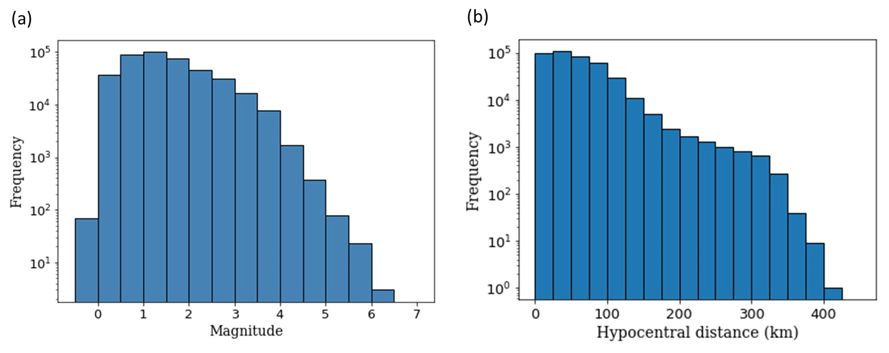
Figure 1 Original distribution (prior to data augmentation) of (a) local magnitudes and (b) hypocentral distances in the chunk of STEAD (Mousavi et al., 2019) data used for training.

As mentioned earlier, we take a local magnitude 5.0 to be the decision boundary between high-magnitude and low-magnitude events. However, the training dataset originally has a magnitude distribution as shown in Fig. 1; this would lead to a high imbalance between the low-magnitude and high-magnitude classes (a ratio of nearly 3300:1). It is widely agreed by the machine learning community that most classifiers assume an equal distribution between the different classes (Batista et al., 2004). Although examples from some domains where models perform reasonably well, even in highly imbalanced datasets, show that there are other factors at play, imbalanced datasets not only are a major hindrance in the development of good classifiers but can also lead to misleading evaluations of the accuracy of the model (Batista et al., 2004). To tackle this imbalance problem, we apply resampling of the data (Krawczyk, 2016) as follows.

• –

  Events with magnitude equal to or above 5.0 are represented 20 times in the dataset by using a shifting window starting from 300 samples to 280 samples before the first P-arrival sample, the window being shifted by 2 samples for each representation. Each of these traces are also flipped; i.e. their polarity is reversed, since it does not affect the magnitude information of the data. Such data augmentation techniques used for images have also been found to be useful for time series data (Batista et al., 2004; Wen et al., 2021).

• –

  For low-magnitude events the following strategy of random undersampling is adopted.

  • 1.

    All events with magnitude between 4.5 and 5.0 are used.

  • 2.

    A total of $\mathrm{1}/\mathrm{3}$ of events with magnitude between 4.0 and 4.5 are used.

  • 3.

    A total of $\mathrm{1}/\mathrm{50}$ of events with magnitude between 2.0 and 4.5 are used.

  • 4.

    A total of $\mathrm{1}/\mathrm{100}$ of events with magnitude less than 2.0 are used.

• –

  A total of $\mathrm{1}/\mathrm{25}$ of the available noise traces are used.

Note that special care is taken to include more events close to the decision boundary (magnitude 5.0) so that the model can learn to differentiate between events of magnitude, say, 4.0 to 5.0, which is more difficult compared to differentiating between events of magnitude, say, 2.0 and 5.0. The corresponding distribution of the different classes is shown in Fig. 2. The validation and test datasets follow a similar distribution. As one can see, in spite of the resampling techniques employed, the high-magnitude class is still under-represented in the dataset, as compared to the other two classes. So, we apply a class weight (Krawczyk, 2016) of $\mathrm{1}:\mathrm{1}:\mathrm{10}$, chosen experimentally, for classes 0, 1 and 2 while training the model. The data are used without instrument response removal. Unlike Lomax et al. (2019) we do not normalise the data. Only the waveform information is provided to the model. Since the dataset includes waveforms from different types of instruments, choosing only one type of instrument would significantly reduce the amount of training data, thereby limiting the learning; therefore we use data from different instruments to train the model.

Figure 2 The distribution of classes in the training dataset obtained by undersampling “noise” (represented by class 0) and “low-magnitude” (represented by class 1) data and applying data augmentation to “high-magnitude” (represented by class 2) events. A similar distribution of classes is seen in the validation and test datasets as well.

2.2 Model architecture and model training

The model architecture (Chakraborty et al., 2021) consists of two sets of 1D convolution (Kiranyaz et al., 2021), dropout (Srivastava et al., 2014) and max-pooling (Nagi et al., 2011) layers, followed by three bi-directional long short-term memory (LSTM) layers (Hochreiter and Schmidhuber, 1997). Convolutional neural networks have often been found to be useful for seismological data analysis as they are capable of extracting temporally independent patterns in the data (features). When combined with LSTMs the temporal relations between these features can be obtained. In applications such as magnitude-based classification of earthquakes, this aids in the effective analysis of signal features as compared to the pre-signal background noise. The dropout layers are used to prevent the model from overfitting, and the max-pooling layer is a method to reduce the data dimensionality so that only relevant features can be retained. The final layer is a softmax layer (Goodfellow et al., 2016), which gives a three-element array of the form [$P_{\mathrm{0}},P_{\mathrm{1}},P_{\mathrm{2}}$], where P_i is the probability of the waveform belonging to the class i (Fig. 3). A detailed description of the model architecture is provided in the caption for Fig. 3.

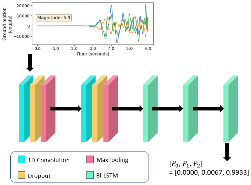
Figure 3 The architecture of the model used to perform the three-class classification. The input to the model is three-component seismic waveform data from a single station. The example shown here corresponds to the case where 3 s of P-wave data is used (the total length of data is, thus, 6 s). The 1D convolution layers have a kernel size of four and eight filters each; the drop rate for each dropout layer is 0.2, and each max-pooling layer reduces the size of the data by a factor of 4; the bi-LSTM layers have dimensions of 256, 256 and 128, respectively. The final layer is a softmax layer that outputs the probability of the trace belonging to classes 0 (noise), 1 (low-magnitude) and 2 (high-magnitude), represented here as P₀,P₁ and P₂, respectively. In this case a probability of 0.9933 is assigned to class 2 for an event with magnitude 5.3; thus, this is a case of correct classification.

The model is trained using an Adam optimiser (Kingma and Ba, 2015), categorical cross-entropy loss (Murphy, 2012) and a batch size of 256. Early stopping (Prechelt, 2012) is used to prevent overfitting, whereby the validation loss is monitored, and the training stops when there is no reduction in it for 20 consecutive epochs. We start with a learning rate of 10⁻³ and reduce it by a factor of 10 if the validation loss does not reduce for 15 consecutive epochs until it reaches 10⁻⁶. The model for the epoch corresponding to the lowest validation loss is retained.

3 Results

To analyse the effect of different lengths of data on the performance of the classifier model, we use the metrics listed below to evaluate the model performance. The metrics are calculated in terms of true positive (TP), true negative (TN), false positive (FP) and false negative (FN) samples.

• Accuracy. The accuracy of a classifier is the proportion of testing samples that are correctly classified. Mathematically, it can be defined as follows:

  $$\begin{array}{}\text{(1)}& \mathrm{accuracy}={\displaystyle \frac{\mathrm{TP}+\mathrm{TN}}{\mathrm{TP}+\mathrm{FN}+\mathrm{TN}+\mathrm{FP}}}.\end{array}$$

• Precision. This is the ratio of the number of times the model correctly predicts a class to the total number of times it predicts that class. Mathematically it is defined as

  $$\begin{array}{}\text{(2)}& \mathrm{precision}={\displaystyle \frac{\mathrm{TP}}{\mathrm{TP}+\mathrm{FP}}}.\end{array}$$

• Recall. This is the ratio of the number of times the model correctly predicts a class to the total number occurrences of that class in the dataset. Mathematically it is defined as

  $$\begin{array}{}\text{(3)}& \mathrm{recall}={\displaystyle \frac{\mathrm{TP}}{\mathrm{TP}+\mathrm{FN}}}.\end{array}$$

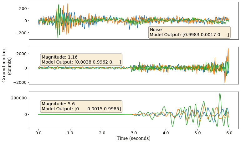
Figure 4 Examples of waveforms that have been correctly classified. In each case the highest probability corresponds to the respective class.

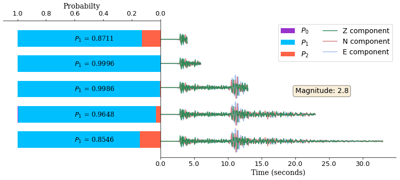
Figure 5 Softmax probabilities for different input lengths of the same waveform, predicted by the models trained on the corresponding lengths of data. The waveform used here corresponds to an event of magnitude 2.8; although the maximum probability corresponds to class 1, the values of these probabilities are different for different data lengths, and there is no clear dependence between the length of the data and this probability.

Figure 4 shows three waveforms (one from each class) that have been correctly classified. The softmax probabilities, as described in Sect. 2.2, are also shown. In each case the highest probability is predicted for the corresponding class. Figure 5 shows the softmax probabilities, predicted by the model for different lengths of the same waveform. Although the waveform is correctly classified in each case, the predicted probabilities are different and show no dependence on the length of input data.

Figure 6 (a) Variation in classifier model performance when different durations (1, 3, 10, 20, 30 s) of P-wave data are used; (b) variation in the classifier model performance when the same model is retrained on the same data (in this case 3 s of P-wave data used) five times. This shows that the variations in the two cases are comparable.

4 Discussions

We investigated the possible factors that might be influencing the model performance. Figure 6a shows the variation in the model performance with respect to the duration of P-wave data used as an input. As we do not tune a random seed during model training (Bengio, 2012; Madhyastha and Jain, 2019), we also looked at the randomness in the performance when the model is trained on the same data five times (Fig. 6b). Thus, we can see that the variation in the results caused by changing the length of data is comparable to the randomness in the results due to random initialisation upon retraining the model on the same data.

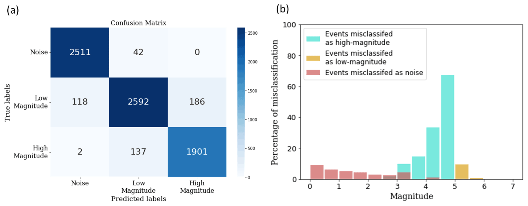
Figure 7 The classification results for a model trained on the 3 s data. (a) The confusion matrix (Ting, 2017) for a model trained and tested on the 3 s data. (b) The misclassification statistics for the same model, for different magnitude values. Note how the highest degree of misclassification happens close to the decision boundary. The percentage of low-magnitude events classified as high-magnitude is much higher than the percentage of high-magnitude events classified as low-magnitude. This is a result of the class weights we used while training the model.

Figure 7 shows the classification statistics for one of the iterations of the model trained on the 3 s data. The events classified as noise tend to be of low magnitude, while the misclassification of low-magnitude events as high-magnitude and vice versa is most pronounced at the decision boundary of 5.0. Another important observation is that the degree of misclassification of low-magnitude events is much higher than the reverse case; approximately 65 % of events with magnitude between 4.5 and 5.0 and 35 % of events with magnitude between 4.0 and 4.5 are classified as high-magnitude, while fewer than 10 % of events with magnitude between 5.0 and 5.5 are classified as low-magnitude; this is intentional as a missed alarm is considered more dangerous than a false alarm in this context (Allen and Melgar, 2019) and is achieved by giving the high-magnitude class more weight during model training.

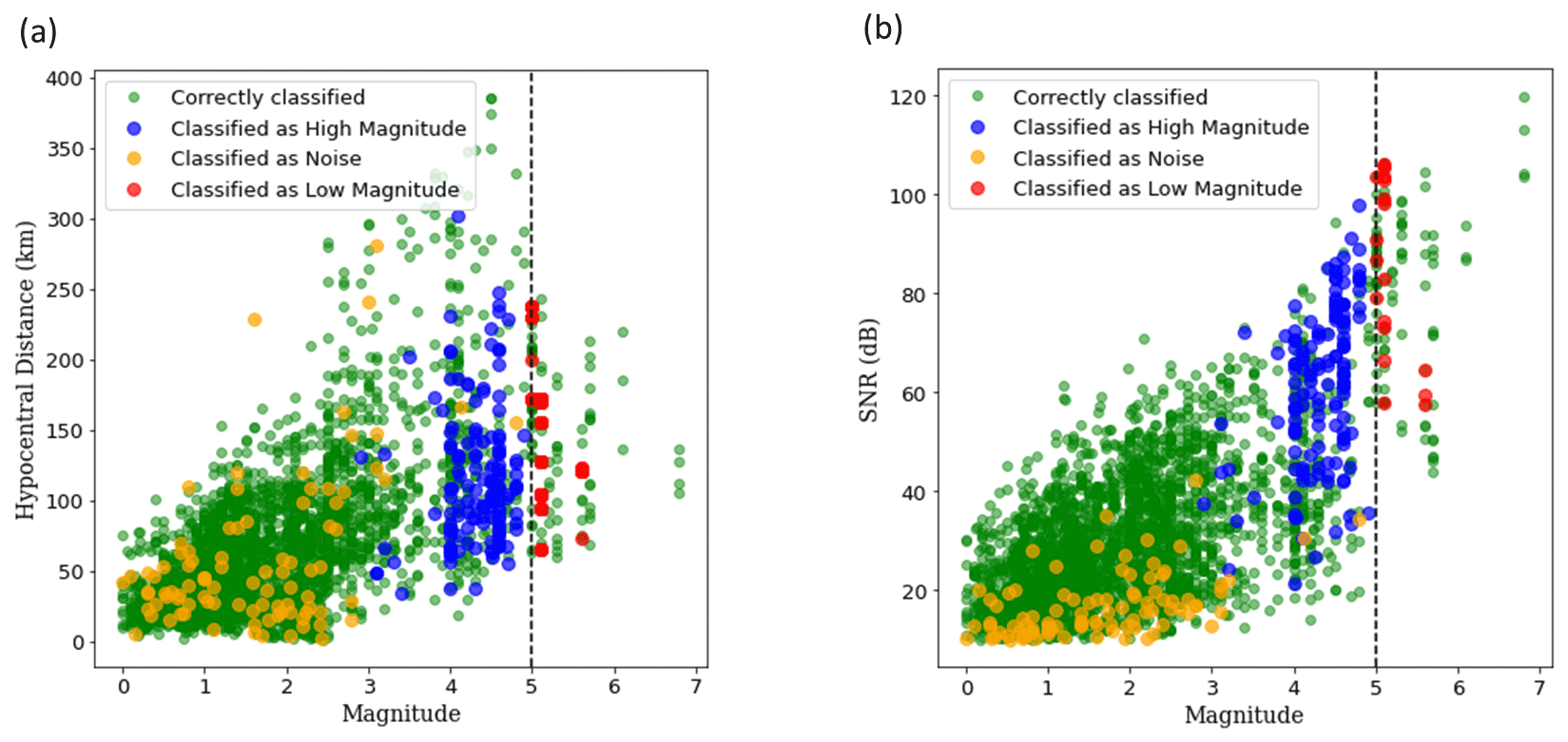
Figure 8 Classification of events with different (a) hypocentral distance and (b) signal-to-noise ratio (SNR). It is observed that the model can correctly classify traces over a range of hypocentral distance and SNR, which exhibits its ability to learn from the frequency characteristics and does not directly learn from amplitude or SNR to some extent. There seems some visible clustering of misclassification of low-magnitude events as noise for SNR below 20 dB.

Figure 8 visualises the classification of events across different hypocentral distance (Fig. 8a) and signal-to-noise ratios (Fig. 8b). We observe that there are instances of correct classification across a wide-range of hypocentral distances and signal-to-noise ratios (SNRs), which means that the model is capable of learning the frequency characteristics of waveforms to some extent and does not directly correlate the amplitude or SNR with magnitude. We do observe some clustering of low-magnitude events classified as noise for SNRs below 20 dB. But for the demarcation between low-magnitude and high-magnitude events the misclassification seems to be close to the decision boundary and spread across a wide range of hypocentral distances and signal-to-noise ratios.

Despite maximising the amount of data on either side of the decision boundary between low and high magnitude, we find some incorrect classifications, most of which lie within a range of 5.0±0.5, as can be seen in Fig. 8. However, considering that sometimes even magnitudes of the same scale reported by different agencies can vary by as much as 0.5 magnitude units (Mousavi and Beroza, 2020), it can be expected that the model would have difficulty in classifying traces close to the decision boundary. In a future version of the model, it might be helpful to treat this as a regression problem instead of classification, thereby providing the model more information about the exact value of the magnitude. The model obtains an overall accuracy ranging between 90.04 % and 93.86 %, which is comparable to the magnitude classification accuracy of 93.67 % achieved by Saad et al. (2020) using data from three seismic stations. This shows great potential in the area of single-station waveform analysis for earthquake early warning.

5 Conclusions

In this study, we present a deep learning model that classifies seismic waveform into three classes: noise, low-magnitude events and high-magnitude events, with events of local magnitude equal to or above 5.0 categorised as “high-magnitude”. We investigate the effect of using different durations of P-wave data to perform the said task and demonstrate that changing the length of the waveform (1, 3, 10, 20 or 30 s after P arrival) has no significant effect on the model performance. We also find that the model classifies most of the data above a magnitude of 4.5 as high-magnitude, even though the decision boundary is chosen at 5.0, due to the higher class weight assigned to high-magnitude events. We obtain an overall accuracy of up to 93.86 %, and we expect this to be very useful in the fast classification of seismological data.