the Creative Commons Attribution 4.0 License.
the Creative Commons Attribution 4.0 License.
 | 16 Feb 2022
Exhumation and erosion of the Northern Apennines, Italy: new insights from low-temperature thermochronometers
Maria Giuditta Fellin
Sean D. Willett
Analysis of new detrital apatite fission-track (AFT) ages from modern river sands, published bedrock and detrital AFT ages, and bedrock apatite (U-Th)/He (AHe) ages from the Northern Apennines provides new insights into the spatial and temporal patterns of erosion rates through time across the orogen. The pattern of time-averaged erosion rates derived from AHe ages from the Ligurian side of the orogen illustrates slower erosion rates relative to AFT rates from the Ligurian side and relative to AHe rates from the Adriatic side. These results are corroborated by an analysis of paired AFT and AHe thermochronometer samples, which illustrate that erosion rates have generally increased through time on the Adriatic side but have decreased through time on the Ligurian side. Using an updated kinematic model of an asymmetric orogenic wedge, with imposed erosion rates on the Ligurian side that are a factor of 2 slower relative to the Adriatic side, we demonstrate that cooling ages and maximum burial depths are able to replicate the pattern of measured cooling ages across the orogen and estimates of burial depth from vitrinite reflectance data. These results suggest that horizontal motion is an important component of the overall rock motion in the wedge, and that the asymmetry of the orogen has existed for at least several million years.
- Article
(5363 KB) - Full-text XML
-
Supplement
(9454 KB) - BibTeX
- EndNote


The Apennine mountains of Italy are an active orogen characterized by contemporaneous extensional and compressional tectonics. In the Northern Apennines, these features are linked to rollback of the Adriatic slab beneath Eurasia, suggested to be active since the Oligocene (Malinverno and Ryan, 1986). The interplay between extension and compression has affected the overall tectonic evolution of the Northern Apennines and, in particular, its exhumational and topographic evolution. Low-temperature bedrock and detrital thermochronology studies have constrained the timing and rates of exhumation at the orogen scale (e.g. Thomson et al., 2010; Malusà and Balestrieri, 2012) and at the regional scale along the extensional Ligurian side of the orogen (e.g. Fellin et al., 2007), and in the frontal fold-and-thrust belt (Adriatic side) (Balestrieri et al., 1996; Carlini et al., 2013; Zattin et al., 2002). Age–elevation profiles and multiple thermochronometers have revealed spatially variable exhumation across and along strike of the orogen, and temporal variability in exhumation rates (Thomson et al., 2010). Although spatial variability is large, the overall pattern of exhumation is consistent with kinematic models of the Apennines as an orogenic wedge, with deformation driven by frontal accretion on the Adriatic margin, and erosion and extension across the mountain belt (Thomson et al., 2010).
In this paper, we augment the thermochronometric data of the range with new detrital thermochronometric data from the Ligurian side of the range to ensure the broadest possible sampling of the thermochronological signal, recognizing that bedrock sampling can miss local regions of anomalous exhumation rate, as was shown from detrital data on the Adriatic side of the orogen (Malusà and Balestrieri, 2012). Published and new data are combined into an analysis of local and regional patterns of exhumation rate through thermal and kinematic modelling. We derive time-averaged erosion rates for individual samples, using two different methods for determining the relevant geothermal gradients. In addition, we calculate erosion rates through time for paired apatite fission-track (AFT) and apatite (U-Th)/He (AHe) samples to compare with results from age–elevation transects that illustrate a change in erosion rates at 4 Ma (Thomson et al., 2010). Our results suggest that the increase in exhumation is restricted to the Adriatic side of the orogen and may have occurred later (∼1–3 Ma), whereas exhumation rates decreased on the Ligurian side at ∼1–5 Ma. Finally, to understand how this pattern of regional erosion rates relates to orogen-scale kinematics of the Northern Apennines, we propose an updated kinematic model that allows for crustal accretion from both frontal accretion and underplating, and variable temperature at the base of the crust.
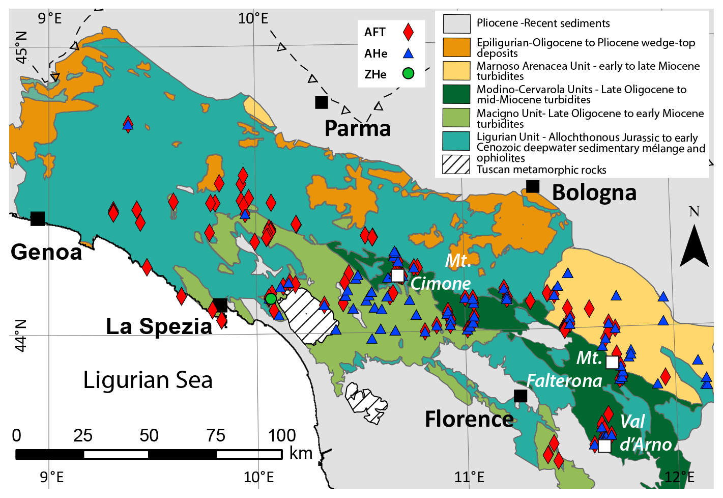
Figure 1Simplified geologic map of the Northern Apennines and locations of published (>10 Ma) bedrock AFT samples (diamonds) (Abbate et al., 1994; Balestrieri, 2000; Balestrieri et al., 1996, 2018; Bonini et al., 2013; Carlini et al., 2013; Fellin et al., 2007; Thomson et al., 2010; Ventura et al., 2001; Zattin et al., 2002), AHe samples (triangles) (Fellin et al., 2007; Thomson et al., 2010), and ZHe sample (circle) (Fellin et al., 2007). Dashed sawtooth lines represent the thrust front buried beneath Po Plain sediments. The following chronostratigraphic divisions are used as minimum depositional ages for the Cenozoic foredeep units: Macigno Unit (Chattian–Aquitanian) (Cita Sironi et al., 2006), Cervarola Unit (Aquitanian–Langhian) (Delfrati et al., 2002), and Marnoso–Arenacea Unit (Burdigalian–Tortonian) (Pialli et al., 2000).
1.1 Geologic and thermotectonic evolution
Development of the Apenninic wedge began during the Eocene between ∼49–42 Ma, due to convergence and southwest-directed subduction of the Adriatic microplate beneath Eurasia (Lustrino et al., 2009). From the Late Oligocene, sediments supplied largely by the Central Alps (Garzanti and Malusà, 2008; Malusà et al., 2016b) were deposited as turbidite sequences into a series of northward-migrating foredeep basins (Macigno, Cervarola, and Marnoso–Arenacea basins) (Fig. 1), which were subsequently uplifted and deformed during the Neogene (Ricci Lucchi, 1986). Until the Pliocene, these Cenozoic foredeep basins were overridden by the Ligurian Unit (Fig. 1), a non-metamorphosed, allochthonous accretionary complex that was thrust over the Cenozoic foredeep deposits as a surficial nappe (Merla, 1952; Pini, 1999). Eocene-to-Pliocene basins formed on top of the Ligurian Unit (epi-Ligurian Unit) (Ori and Friend, 1984; Cibin et al., 2001), which record discontinuous deposition of shallow-marine and continental sediments (Ricci Lucchi, 1986), and presently exist as erosional remnants above the Ligurian Unit. Today, the Ligurian and epi-Ligurian units are the highest structural units exposed in the Northern Apennines.
The onset of near-surface exhumation is constrained by the present extent and depositional ages of the epi-Ligurian units on the Adriatic side (Fig. 1), which are commonly not younger than the Tortonian in the NW of the study area; however, to the ESE, near Bologna, they can be as young as the Pliocene (Cibin et al., 2001). The onset of near-surface exhumation in the Northern Apennines is suggested to have begun earlier than 14 Ma, during the Tortonian (Ventura et al., 2001), although the timing of the onset is debated. However, it is clear that rapid exhumation began at 8–9 Ma on the Ligurian side (Balestrieri et al., 1996), and at 4–7 Ma near the divide between the Ligurian and Adriatic sides, based on the ages and younging trend in AFT and AHe thermochronometers <10 Ma (Fig. 2) (Thomson et al., 2010).
The first evidence for emergent topography in the Northern Apennines is documented in the early Pliocene by lacustrine deposits in an intermontane extensional basin located within the Magra River catchment (Fig. 3) (Bertoldi, 1988; Balestrieri et al., 2003). These deposits are overlain by late Pliocene alluvial conglomerates that contain metamorphic pebbles sourced from the Apuan Alps metamorphic dome (white, hatched area in Fig. 3a), indicating that the Apuan Alps were emergent at this time (Fellin et al., 2007). The onset of topographic relief then migrated eastward (Abbate et al., 1999; Carlini et al., 2013; Thomson et al., 2010), recorded by increased rock uplift rates at the drainage divide during the Pleistocene (Balestrieri et al., 2003), and the formation of Pleistocene-to-Holocene deformed fluvial terraces near the Adriatic mountain front (Picotti and Pazzaglia, 2008; Wegmann and Pazzaglia, 2009; Wilson et al., 2009).
Cooling ages in the Northern Apennines are primarily limited to AFT and AHe methods (Balestrieri et al., 1996; Ventura et al., 2001; Zattin et al., 2002; Balestrieri et al., 2003; Fellin et al., 2007; Thomson et al., 2010; Malusà and Balestrieri, 2012; Carlini et al., 2013; Balestrieri et al., 2018), as the region is dominated by sedimentary rocks (Fig. 1) that have experienced relatively low burial temperatures of less than 200–250 ∘C (Reutter et al., 1983). Non-reset clastic rocks in the Northern Apennines are commonly exposed close to the frontal thrust zone, near the mountain front, and at high elevations (e.g. Zattin et al., 2002; Thomson et al., 2010; Carlini et al., 2013).
Maximum burial depths of rock across the Northern Apennines are constrained most commonly from vitrinite reflectance data (Fig. 2; Reutter et al., 1983; Ventura et al., 2001; Botti et al., 2004; Carlini et al., 2013), which is a proxy for burial temperatures recorded by organic particles, and is expressed as Ro (%). Higher Ro values generally reflect higher burial temperatures. Ro increases steadily from NE to SW in the Northern Apennines, with maximum Ro values near the Ligurian coastline, as shown along the swath profiles in Fig. 2. This pattern of Ro values was interpreted to reflect NE-directed Miocene thrusting of the Ligurian Unit, which buried the underlying Cenozoic foredeep deposits (Reutter et al., 1983). Ro values also decrease along strike of the orogen from NW to SE (Fig. 2), illustrating that maximum burial depths also decrease towards the SE. This pattern was in turn interpreted to reflect the shape of the Ligurian Unit as a wedge that thinned towards the east (Zattin et al., 2002) and thus resulted in shallower burial depths for the underlying Cenozoic foredeep deposits.
2.1 Detrital AFT thermochronology
Bulk samples of modern sand were collected from six rivers on the Ligurian side of the Northern Apennines (Fig. 3a) and are representative of the Macigno, Cervarola, Apuan Alps, and Ligurian units (Fig. 1). As some Ligurian catchments (Magra and Serchio rivers) contain basins with Pliocene sediments, additional samples were collected in tributaries above these basins to avoid sampling the younger, post-orogenic sediments.
Samples were processed according to the external detector method for AFT dating, using standard methods. Bulk samples were first sieved with a 1.5 mm mesh, and heavy minerals were concentrated using standard techniques, involving the use of the Wilfley table and of heavy liquids. We separated the apatite from lighter minerals using a heavy liquid with a density of 3 g cm−3, and subsequently separated the apatite from heavier minerals (e.g. zircon, rutile, and monazite) using a heavy liquid with a density of 3.3 g cm−3. A magnetic separator was used to further concentrate the apatite. Apatite grains were then poured onto glass slides, carefully avoiding any potential selection of grains due to differences in size and shape. The grains were subsequently embedded in cold epoxy and polished to expose the internal surfaces of the apatite grains. For each sample, we counted all countable grains, which specifically refers to any grains that expose a section parallel to the C axis, independently of whether it has zero or more spontaneous tracks. Multiple mounts per sample were produced to maximize the number of datable grains, and we aimed to date at least 100 grains per sample. However, only 37, 87, and 77 apatite samples were countable in samples Lima1 (6), Bisenzio (7), and Pescia (8), respectively, whereas the high number of countable apatite grains in samples Vara (1) and Magra1 (3) allowed us to date 150 grains in each sample.
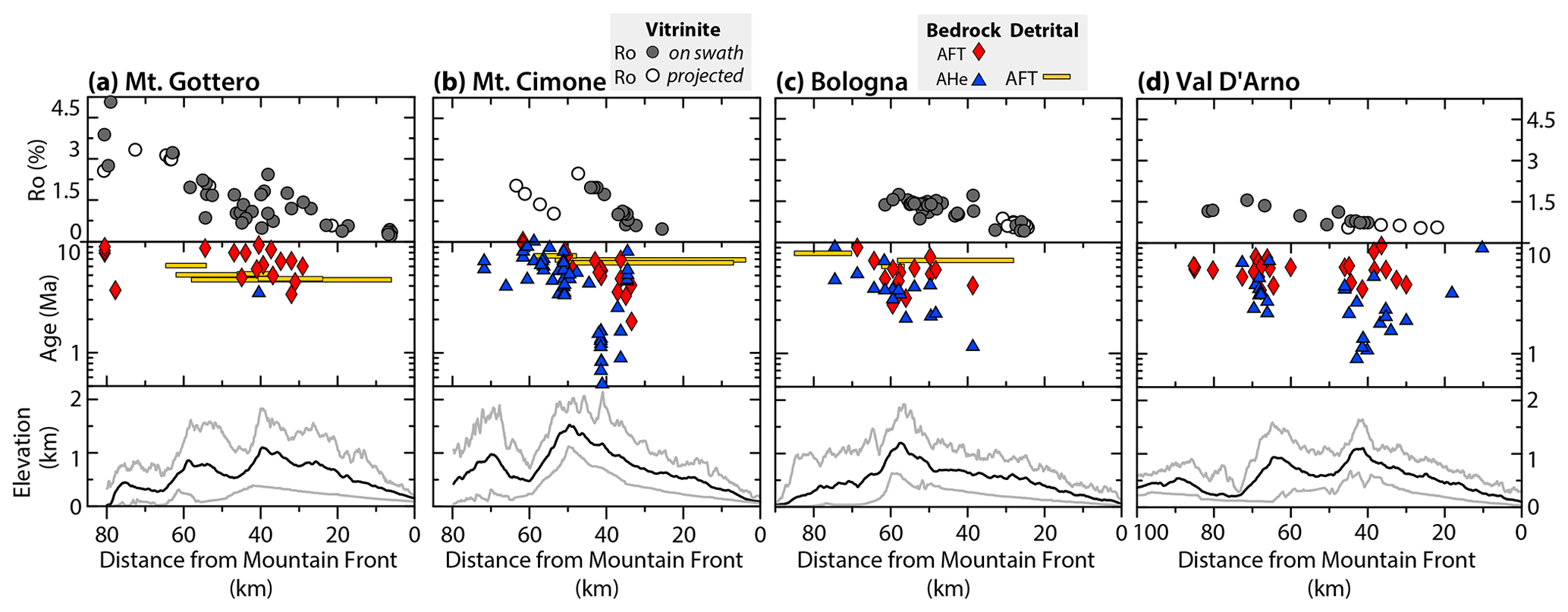
Figure 2Published vitrinite reflectance (Botti et al., 2004; Carlini et al., 2013; Reutter et al., 1983; Ventura et al., 2001), published bedrock cooling ages (Abbate et al., 1994; Balestrieri, 2000; Balestrieri et al., 1996, 2018; Bonini et al., 2013; Carlini et al., 2013; Fellin et al., 2007; Thomson et al., 2010; Ventura et al., 2001; Zattin et al., 2002) and new detrital cooling ages, and topography plotted along (a) Mt. Gottero, (b) Mt. Cimone, (c) Bologna, and (b) Val D'Arno swath profiles. Profile locations are shown in Fig. 3a. Top row: filled circles are vitrinite reflectance samples located within the 30 km wide swath profile; empty circles are located outside of swath profile line and were projected onto the line. Middle row: cooling ages corrected for topography for bedrock AFT (red diamonds), and AHe (blue triangles). Detrital AFT samples (yellow rectangles) were not corrected for topography. Bottom row: mean elevation (thick black line) and minimum and maximum elevation (light grey lines).
Apatite grains were etched in 5.5 N HNO3 for 20 s at 21 ∘C. AFT ages were measured and calculated using the external-detector and the zeta-calibration methods (Hurford and Green, 1983) with International Union of Geological Sciences (IUGS) age standards (Durango and Fish Canyon apatites) (Hurford, 1990). The analyses were subjected to the χ2 test (Galbraith, 1981) to assess whether the sample age distributions were overdispersed; a probability of less than 5 % denotes mixed distributions.
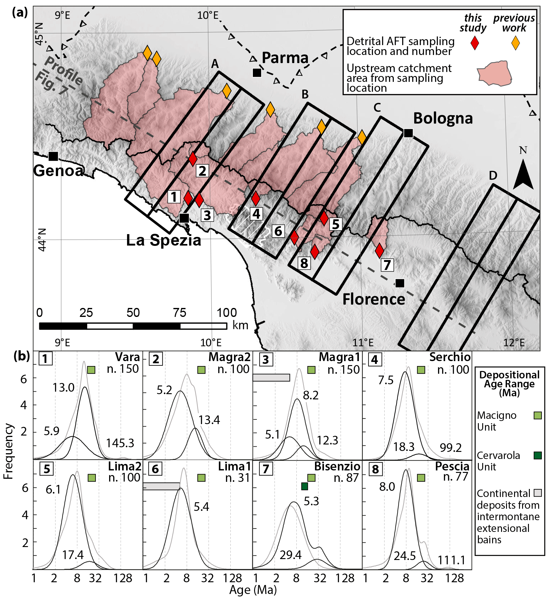
Figure 3(a) Location map for detrital samples. Detrital AFT samples from this study are illustrated as red diamonds, and published detrital AFT samples (Malusà and Balestrieri, 2012) are shown as yellow diamonds. Numbers in the white squares correspond to the age population plots shown in panel (b). (c) Peak distribution curves (black curves), total probability density functions (PDFs) (grey curves), and peak ages (Ma) for all sampled Ligurian catchments. Catchment name and sample number (where applicable), and number of dated grains (n.) are given in the top right corner of each figure panel. Coloured rectangles in each plot give the range of stratigraphic ages for the youngest exposed Cenozoic foredeep units (Fig. 1) in the respective upstream catchment area. We also indicate the age range of the Pliocene–Pleistocene continental deposits, as these are potential sources of detrital apatite recycled from the Cenozoic foredeep units or from the Apuan Alps metamorphic rocks.
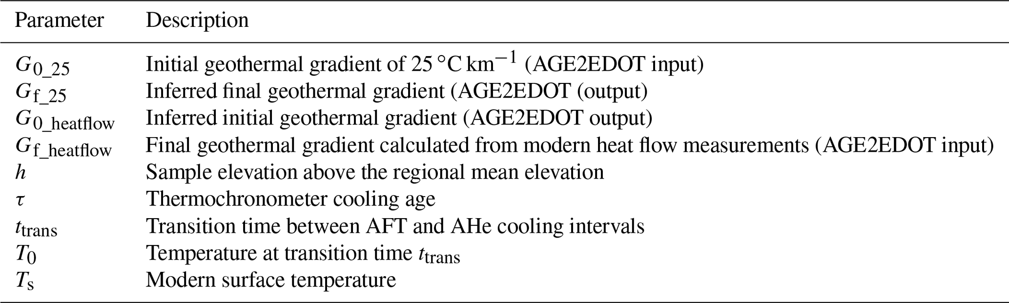
Table 1Definitions of thermal parameters used in the erosion rate analysis.
We determined age populations for detrital samples based on dominant age peaks identified with the Binomfit programme (Brandon, 2002), which is well suited for AFT data with low spontaneous track density. In order to estimate the degree of resetting of the detrital age populations relative to the Apenninic orogenic event, we compared the detrital cooling ages with minimum depositional ages of the Cenozoic foredeep units exposed in the drainage areas (Figs. 1 and 3b).
2.2 Erosion rate analysis
We compiled ages from new and existing detrital AFT samples (23), bedrock AFT samples (139), AHe samples (135), and zircon (U-Th)/He (ZHe) samples (26) (Supplement Tables S1–S4) (Abbate et al., 1994; Balestrieri et al., 1996; Ventura et al., 2001; Zattin et al., 2002; Balestrieri et al., 2003; Fellin et al., 2007; Thomson et al., 2010; Malusà and Balestrieri, 2012; Carlini et al., 2013). As the Apuan Alps have an erosional history different from the rest of the Northern Apennines (Balestrieri et al., 2003; Fellin et al., 2007), we removed these samples from our compilation of thermochronometric ages.
We converted ages to erosion rates using a half-space cooling model and a closure temperature concept (Willett and Brandon, 2013). This model has the advantage of including an accurate representation of the transience associated with whole lithosphere geotherms. Reset ages were converted to erosion rates using closure temperatures specific to each thermochronometer, although this is a simplification of diffusional daughter product loss that neglects effects associated with complex cooling histories. For monotonic cooling histories, the measured age of the sample is represented by the time needed for a rock to move from the closure depth to the surface (e.g. Reiners and Brandon, 2006).

Figure 4Schematic of paired-age erosion rate analysis, illustrating the theoretical temperature path through time for a sample with paired AFT and AHe cooling ages, given the thermal parameters described in the text; ė represents the erosion rate for each cooling interval.
The conversion to erosion rates was performed using the AGE2EDOT programme (Willett and Brandon, 2013), which estimates an erosion rate from a closure temperature and a geotherm obtained by solution of the 1-D thermal advection–diffusion problem for a lithospheric column subjected to a constant rate of erosion. Thermochronometric data required for the calculations include the measured ages and kinetic parameters from which a closure temperature is calculated. In addition, the thermal initial conditions and boundary conditions, as well as thermal parameters, must be specified for each sample site.
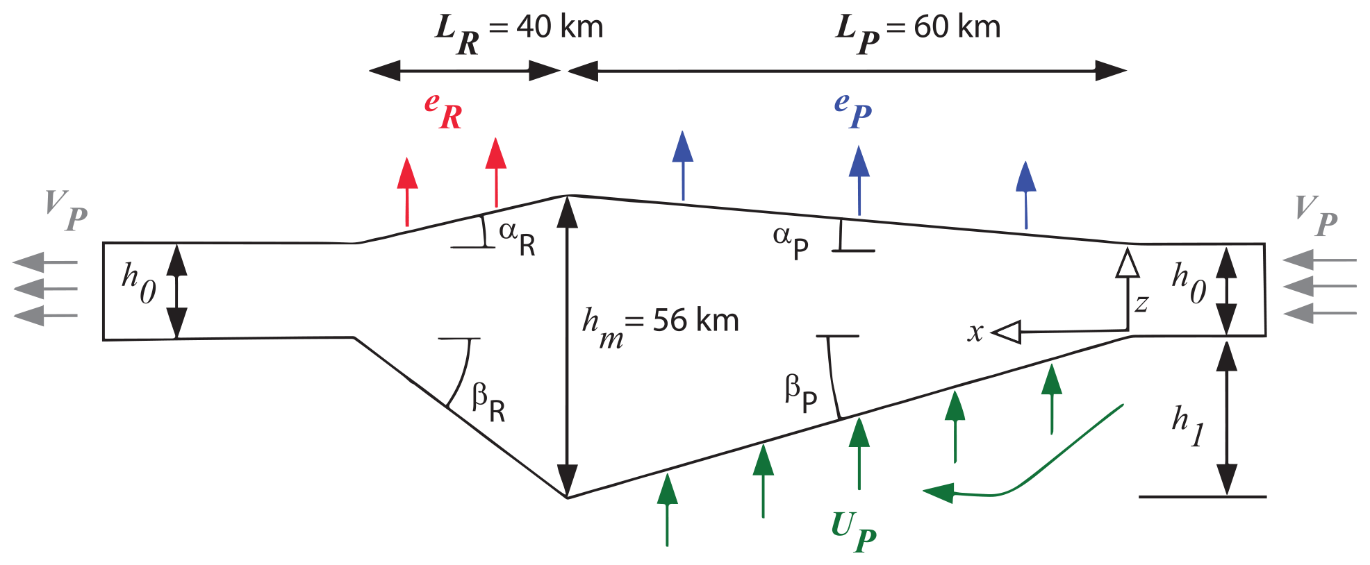
Figure 5Kinematic model of the Northern Apennines as an orogenic wedge with internal deformation driven by frontal and basal accretion and surface erosion. Mass is balanced to maintain a steady size, and internal deformation is calculated to be consistent with boundary conditions.
For the kinetic parameters for AHe, we assumed grain sizes of 45 µm, given that sizes of dated grains are not reported by previous studies, and that a grain size of 60 µm is larger than the mean size of detrital apatite grains that are typically dated in the Northern Apennines. Thermal parameters (see definitions in Table 1) include an estimate for the onset age of erosion (t1); the sample elevation, given as an elevation above a regional mean (h); surface temperature (Ts); and either an initial geothermal gradient (G0) or the final geothermal gradient (Gf). Only one estimate of the geothermal gradient is needed, but we took two approaches, as will be discussed below. To calculate Ts, we adjusted a base temperature value for the elevation of each sample, given a lapse rate of 5 ∘C km−1. For the base temperature, we used a modern surface temperature of 13.8 ∘C, which represents the calculated yearly average for an elevation of 53 m at Bologna from 1813–2004 (NOAA Global Temperature Summary of the Year dataset).

Figure 6Comparison of initial geothermal gradients (G0) and final geothermal gradients (Gf) for AFT samples (a–c) and AHe samples (d–f). (a, d) Comparison of G0_heatflow and Gf_heatflow. (b, e) Comparison of Gf_heatflow with Gf_25. (c, f) Comparison of erosion rates derived from Gf_heatflow measurements versus erosion rates derived from imposed G0_25.
The geothermal gradient is the most important parameter incorporated into the erosion rate analysis and is also the largest source of uncertainty. It can be specified either as a final geothermal gradient (Gf), which is the present geothermal gradient at the surface, or as an initial geothermal gradient (G0) that is assumed to be constant with depth at the onset of exhumation (Willett and Brandon, 2013). We calculated and compared erosion rates derived using two approaches. In the first method, we imposed a spatially constant G0 of 25 ∘C km−1 (G0_25) (Balestrieri et al., 2003; Ventura et al., 2001; Zattin et al., 2002). In the second method, we assumed that the present-day geothermal gradient (Gf) matches the geothermal gradient calculated from geothermal heat flow measurements. We converted the heat flow measurements to a Gf (Gf_heatflow) using a spatially constant thermal conductivity value for sandstone (2 W mK−1). Heat flow values were extracted from contour maps that interpolate geothermal well data (Pauselli et al., 2019; della Vedova et al., 2001). The della Vedova et al. (2001) heat flow map covers the entire study area, whereas the Pauselli et al. (2019) map covers the area south of 44.5∘ N and includes only the Bisenzio River (Fig. 3) within the study area. Because the heat flow map of della Vedova et al. (2001) is based on fewer geothermal well measurements relative to the Pauselli et al. (2019) map, we consider the della Vedova et al. (2001) interpolation to have higher uncertainties. Thus, where the Pauselli et al. (2019) map was available, a heat flow value was selected from this map. Otherwise, a heat flow value was selected from the della Vedova et al. (2001) map.
The modelling procedure described above was applied to all ages, assuming that erosion initiated over the entire region at 10 Ma. The resulting erosion rate applies from the onset of exhumation at 10 Ma to the present and reflects the time-averaged erosion rate that is constrained to pass through the closure temperature at the cooling age and with a cooling rate commensurate with the average erosion rate. Thus, this method is limited to a single, average erosion rate. However, changes in exhumation rates through time in the Northern Apennines are supported by several lines of evidence, particularly by age–elevation transects (AETs). In fact, AETs from the existing literature illustrate differences along the age–elevation slope for a single thermochronometer (as in Balestrieri et al., 1996) or among age–elevation slopes for multiple thermochronometers (as in Thomson et al., 2010).
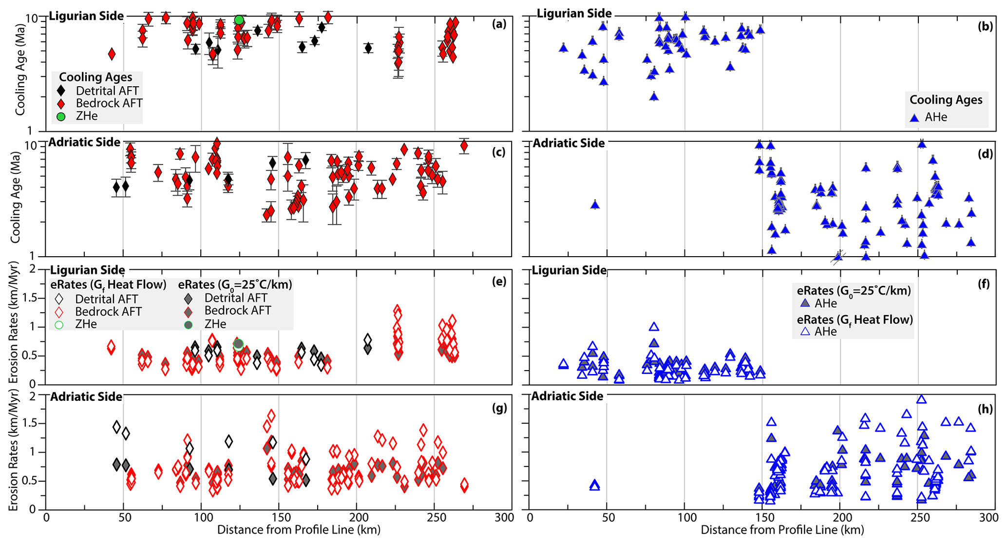
Figure 7Profile parallel to the orogen strike (profile location shown in Fig. 3a) illustrating cooling ages along the Ligurian side for (a) AFT and ZHe data and (b) AHe data, and along the Adriatic side for (c) AFT and ZHe data and (d) AHe data. Erosion rates along the Ligurian side for (e) AFT and ZHe data and for (f) AHe data, and along the Adriatic side for (g) AFT and ZHe data and for (h) AHe data. In panel (d), individual AHe symbol dated to >1 Ma is illustrated with a double grey slash.
It is possible to use AGE2EDOT in an incremental manner, allowing us to use paired thermochronometers analysed from a single sample. In this case, the temporal range of exhumation is bracketed by the AFT and AHe ages, with independent erosion rates determined from each age, thus resolving two time intervals (Willett et al., 2021). In principle, this violates the assumption of a constant rate of cooling implicit to the use of the closure age concept, but provided that the transition between erosion rate intervals is not close to either age, the error will be small. We analysed 30 available paired ages to detect temporal changes in erosion rate. For the paired-age analysis, the exhumation path is divided into two segments: the first segment extends from the onset of exhumation to a specified transition time (ttrans) after cooling through the AFT system, and the second segment extends from this transition time to the present, thus passing through the AHe age in this second interval (Fig. 4). We derive an erosion rate for each of these time segments by analysing each segment with AGE2EDOT, linking the two solutions at ttrans. The solutions are matched by noting the depth and temperature of the sample at ttrans, based on the erosion rate in the second interval, and using this and the geothermal gradient at ttrans as the boundary conditions for calculations of the first interval (Fig. 4).
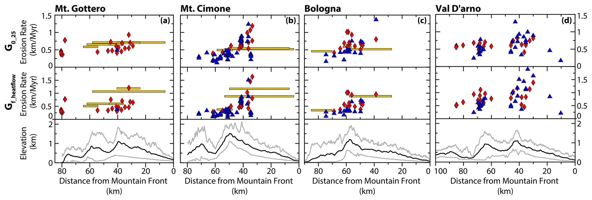
Figure 8Erosion rates for AHe, bedrock AFT, and detrital AFT thermochronometers calculated from G0_25 (top row, a–d) or calculated with Gf_heatflow (middle row, a–d). The length of the detrital AFT boxes reflects the distance from the sample location to the catchment headwaters where the erosion rate is valid. Swath profile locations are shown in Fig. 3a. In the Bologna swath profile, one AHe sample could not be resolved for an erosion rate with Gf_heatflow.
The difference in age between some of our paired ages is less than 1 Ma but larger than 0.5 Ma, so we set the transition at 0.5 Ma before the AHe closure for all samples (i.e. the AHe cooling age plus 0.5 Myr), in order to allow the onset of advection to precede the AHe closure (Fig. 4). Calculation of the erosion rate over the second interval requires the modern surface temperature (Ts); the sample elevation above the regional mean (h); the AHe cooling age (τ); the final geothermal gradient as derived from heat-flow measurements (Gf_heatflow); and the length of the time interval (ttrans), calculated as the AHe age plus 0.5 Myr. The erosion rate is then solved from these data and the kinetic parameters.
To calculate the erosion rate for the first interval, we also require the temperature at ttrans (T0) (Fig. 4); the sample elevation above the regional mean (h); the sample AFT age (τ), and the onset age of erosion, taken as 10 Ma. To match solutions at ttrans, we simply reduce the age by ttrans, and reduce the elevation by the amount of exhumation that occurred during the second interval. We take the initial geothermal gradient obtained from the model for the second interval as the final condition for the first interval.
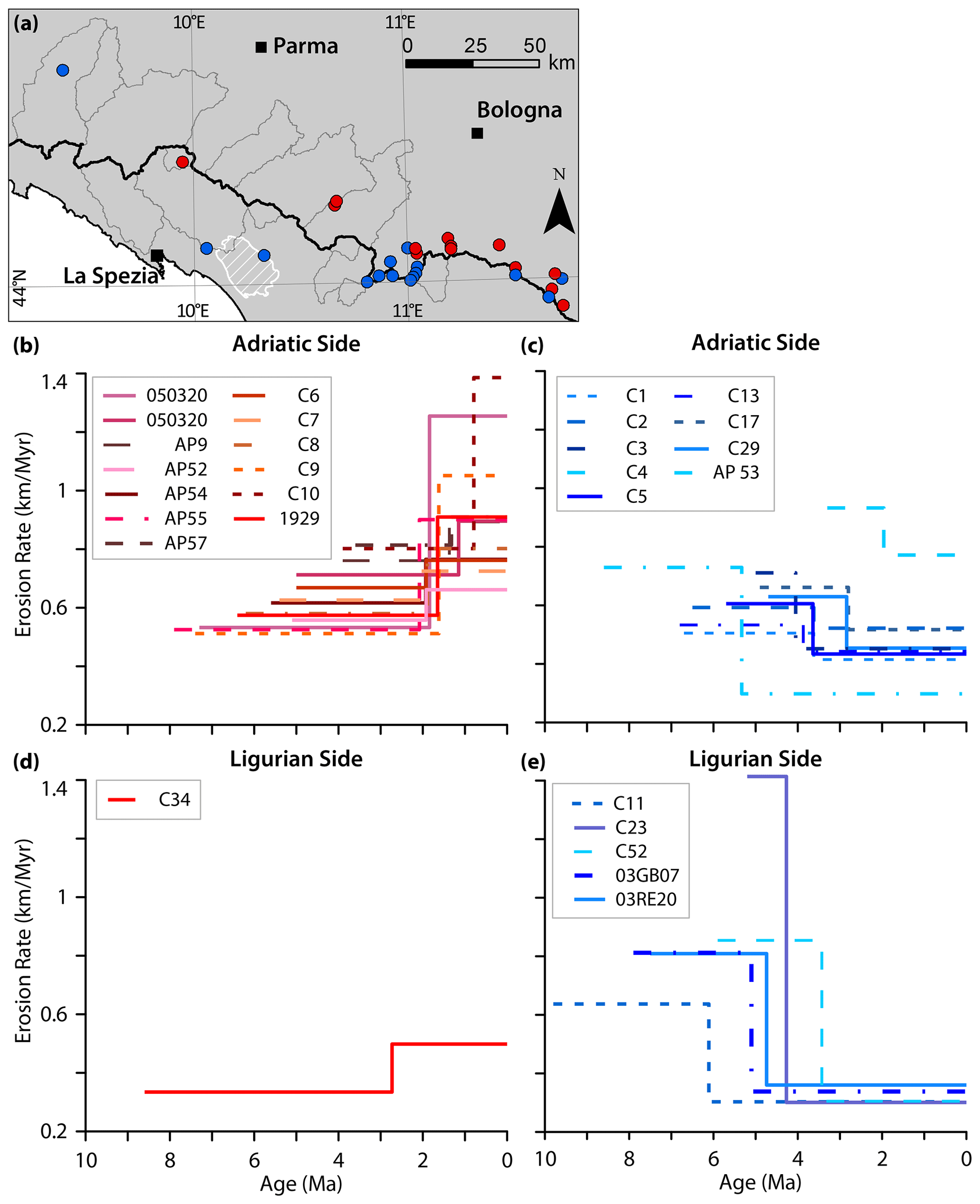
Figure 9Erosion rates through time from paired AFT and AHe age samples on the Adriatic side for (b) increasing erosion rates and (c) decreasing erosion rates, and on the Ligurian side for (d) increasing erosion rates and for (e) decreasing erosion rates. Inset map (a) shows the locations of paired thermochronometer age samples (circles). Red circles indicate locations where the erosion rate through time is increasing, and blue circles indicate locations where the erosion rate through time is decreasing.
2.3 Kinematic model
We used a range of kinematic and thermal parameters applicable to the Northern Apennines to characterize a 1-D kinematic model that aims to (1) model the path of rock particles from accretion into the wedge to their erosion at the surface, (2) calculate uplift and horizontal rock velocities across the wedge, (3) predict reset cooling ages for AHe, AFT, and ZHe thermochronometers, and (4) calculate maximum burial depths across the model. Here, we describe the model geometry and the kinematic and thermal parameters used to constrain the model.
The kinematic model approximates the Northern Apennines as a doubly tapering, asymmetric wedge, given the geometric parameters illustrated in Fig. 5. The Adriatic and Ligurian sides of the orogen are defined as the accreting prowedge and non-accreting retrowedge of the orogen, respectively (e.g. Willett et al., 2001). The geometry of the wedge is defined by surface and basal angles for the prowedge (αP and βP) and retrowedge (αR and βR). The lengths of the prowedge (LP) and retrowedge (LR) are 60 and 40 km, respectively, based on average widths measured from a Shuttle Radar Topography Mission (SRTM) 90 m digital elevation model (DEM). The maximum crustal thickness is 56 km (Spada et al., 2013), the maximum elevation is 2 km, and the thickness of the accreted crust is 20 km, partitioned between frontal accretion (h0=10 km) and prowedge basal accretion (h1=10 km). We assume no retrowedge accretion (h2=0).
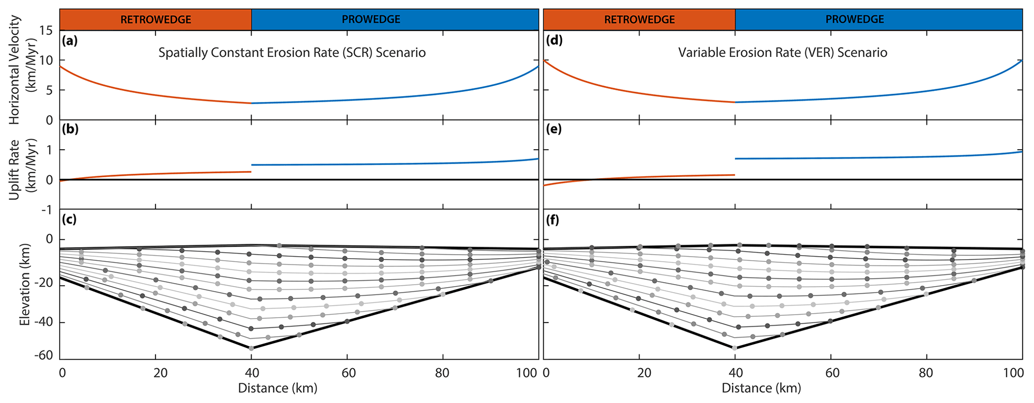
Figure 10Kinematic model results for the spatially constant erosion rate (SCR) scenario (a–c) and the variable erosion rate (VER) scenario (d–f). (a, d) Predicted material horizontal velocities across the orogenic wedge and (b, e) predicted uplift rates across the wedge. (c, f) Material motion paths (lines within wedge) and particle positions and paths, equally spaced in time (solid, coloured circles).
Closure depths were calculated using the closure temperature for each thermochronometer, divided by a spatially and temporally constant geothermal gradient. Closure temperatures are given with AHe of 70 ∘C (Farley, 2000), AFT of 110 ∘C, (Wagner and Van Den Haute, 1992), and ZHe of 180 ∘C (Farley, 2000). Excluding the Apuan Alps samples, we used the full set of unique sample locations in our field area (Tables S1–S4) to calculate an average Gf_heatflow=36.4 ∘C km−1 and closure depths for the ZHe (4.9 km), AFT (3.0 km), and AHe (1.9 km) thermochronometers.
Material is accreted to the wedge through thrusts slices in the upper plate (frontal accretion) or is offscraped from the subducting plate at depth (underplating). Material motion is constrained by balancing frontal and rearward fluxes, underplating, and erosion. We prescribe a compressional prowedge and an extensional retrowedge, where horizontal velocities decrease along the prowedge and increase along the retrowedge as a function of distance. The vertical rock velocity is also variable with depth and is defined as the sum of the erosion rate and a component of crustal thickening driven by accretion.
The velocities in the model are defined as follows: plate subduction velocity (VP), prowedge underplating velocity (UP), prowedge erosional velocity (eP), and retrowedge erosional velocity (eR). The plate subduction velocity, or convergence rate, for the Northern Apennines is suggested to be driven entirely by slab rollback, so we used estimates of slab rollback to parameterize the convergence rate. Slab rollback rates are on the order of ∼6–20 km Myr−1 in this region of the Apennines (Faccenna et al., 2014; Malusà et al., 2015; Rosenbaum and Piana Agostinetti, 2015), so we run the model using these minimum and maximum values as end-member scenarios. We also vary the spatial pattern of erosion rates in the model using two model assumptions: (1) a constant erosion rate across the orogenic wedge and (2) a higher erosion rate on the prowedge relative to the retrowedge. Since the model represents a 1-D cross section through the Northern Apennines, all velocities and rates specified in this model are assumed to reflect motion within the direction of the wedge (i.e. perpendicular to the strike of the orogen).
Table 2Central ages and AFT dataset details.
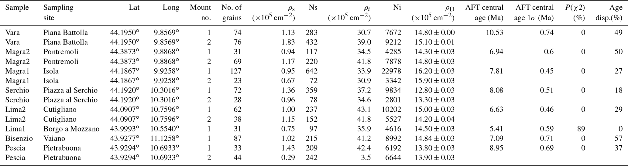
ρs: spontaneous track density. ρi: induced track density in external detector. ρD: induced track density in external detector adjacent to dosimeter glass. Age disp: age dispersion. Ni: number of counted induced tracks. Ns: number of counted spontaneous tracks.
Table 3Peak ages with standard error and size of major peaks (%).
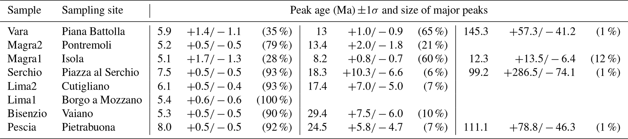
3.1 Detrital AFT cooling ages
New detrital AFT (8) sample ages are given in Fig. 3b and Tables 2–3. Central ages vary from 5.4 ± 0.6 to 10.5 ± 0.7 Ma, and single-grain ages show a wide range of values from 5.1 to 145.3 Ma. All samples except Lima1 show at least two distinct age populations, with minimum age peaks between 5.1 and 8 Ma. All minimum age peaks are younger than the stratigraphic ages of units within the catchment (Fig. 3b) (Cita Sironi et al., 2006; Delfrati et al., 2002; Pialli et al., 2000), with the exception of Magra1. This site contains Plio-Pleistocene deposits exposed in its catchment that are younger than the minimum age peak, but these are locally derived sediments, and the sedimentary bedrock has stratigraphic ages older than the young peak.
In the five southern samples (Serchio, Lima1, Lima2, Pescia, and Bisenzio), the youngest peaks represent the largest age populations and are similar to the sample central ages. The three northern samples (Vara, Magra1, Magra2) show two common age populations at 5–6 and at 12–13 Ma and have central ages older than the minimum peak ages, due to a large proportion of older grains.
3.2 Geothermal gradients and erosion rates
We report initial geothermal gradients (G0) and final geothermal gradients (Gf) using the two approaches described in the methods. Given a G0=25 ∘C km−1 common to all samples, Gf_25 ranges from 27.4 to 55.2 ∘C km−1 for AHe samples (Table S5) and ranges from 31.2 to 49.7 ∘C km−1 for AFT samples (Table S6). Using the second method based on modern heat flow measurements, G0_heatflow for AHe samples ranges from 9.3 to 42.2 ∘C km−1 (Table S5) and ranges from 12.4 to 38.0 ∘C km−1 for AFT samples (Table S6). Relative to the Gf_25, Gf_heatflow derived from Pauselli et al. (2019) are consistently lower, where all samples lie left of the 1:1 trendline for AHe samples (Fig. 6e) and all but one lie left of the 1:1 trendline for AFT samples (Fig. 6b). In contrast, Gf_heatflow derived from della Vedova et al. (2001) are highly variable, although the majority lie to the right of the 1:1 line for both AHe (Fig. 6e) and AFT (Fig. 6b) samples, indicating that these values are higher relative to Gf_25.
Erosion rates calculated using the two methods for estimating geothermal gradients also illustrate different trends for the della Vedova et al. (2001) and Pauselli et al. (2019) heat flow estimates. Erosion rates derived from G0_25 plotted against erosion rates derived from della Vedova et al. (2001) Gf_heatflow lie mostly on the 1:1 trendline for both AFT and AHe samples (Fig. 6c, f) and are thus similar. In contrast, erosion rates calculated with Pauselli et al. (2019) Gf_heatflow are lower relative to erosion rates derived from G0_25 but always by a factor of less than 2 (Fig. 6c, f).

Figure 11Closeup (vertical axis only) of kinematic model shown in Fig. 10. Left and right panels represent the spatially constant erosion rate (SCR) and variable erosion rate (VER) model setups, respectively. (a, d) Predicted age of thermochronometers with distance along the wedge. (b, e) Predicted maximum burial depths for each particle path. (c, f) Material paths in upper 8 km of kinematic model. Coloured lines illustrate closure depths for AHe, AFT, and ZHe thermochronometers.
Here, we present the erosion rate results for the Adriatic and Ligurian sides, given the two methods used for constraining the modern geothermal gradient, and by illustrating the data with two perspectives: (1) along a profile oriented parallel to the orogen strike (Fig. 7, location shown in Fig. 3) and (2) along swath profiles oriented perpendicular to the orogen strike (Fig. 8). Calculated with G0_25, erosion rates inverted from AFT bedrock ages (Table S6; Figs. 7e, g, top row) vary between 0.41 and 1.19 km Myr−1 on the Adriatic side (Fig. 7g) and between 0.36 and 0.84 km Myr−1 on the Ligurian side (Fig. 7e). The highest erosion rates on the Ligurian side are located in the Macigno Unit near the Apuan Alps, whereas the highest rates on the Adriatic side are located near the drainage divide (Cervarola Unit; top row, Fig. 8). AFT bedrock erosion rates across the divide are similar or slightly higher on the Adriatic side (Figs. 7e, g, 8, top row). AFT detrital erosion rates are similar to bedrock AFT rates, which also exhibit erosion rates that are higher on the Adriatic side (top row, Fig. 8). Erosion rates derived from AHe ages (Table S5) range between 0.14 and 1.39 km Myr−1 on the Adriatic side and between 0.14 and 0.74 km Myr−1 on the Ligurian side. AHe erosion rates on the Adriatic side are more variable relative to the Ligurian side, particularly in the southeast region of the field area (Fig. 7f, h). Similar to the bedrock AFT erosion rates, the highest AHe erosion rates are found on the Adriatic side near the drainage divide and are lowest near the Ligurian coastline (top row, Fig. 8).
Calculated with Gf_heatflow, the pattern of erosion across the drainage divide is similar to the pattern for erosion rates calculated with G0_25 (middle row, Fig. 8). On the Adriatic side, erosion rates inverted from AFT bedrock and detrital ages vary between 0.34 and 1.63 km Myr−1 and between 0.88 and 1.44 km Myr−1, respectively. On the Ligurian side, AFT bedrock erosion rates vary between 0.26 and 1.28 km Myr−1, and detrital AFT erosion rates vary between 0.34 and 0.78 km Myr−1. Erosion rates derived from AHe ages range from 0.17 to 1.92 km Myr−1 on the Adriatic side and from 0.10 to 1.02 km Myr−1 on the Ligurian side. Detrital AFT erosion rates on the Adriatic side are higher relative to the Ligurian side, regardless of the method used for constraining the geothermal gradient. However, calculated from Gf_heatflow, detrital AFT erosion rates on the Adriatic side are up to a factor of 2 higher than erosion rates calculated with G0_25 (Fig. 8).
Table 4Erosion rates and parameters for paired AFT–AHe thermochronometer samples.
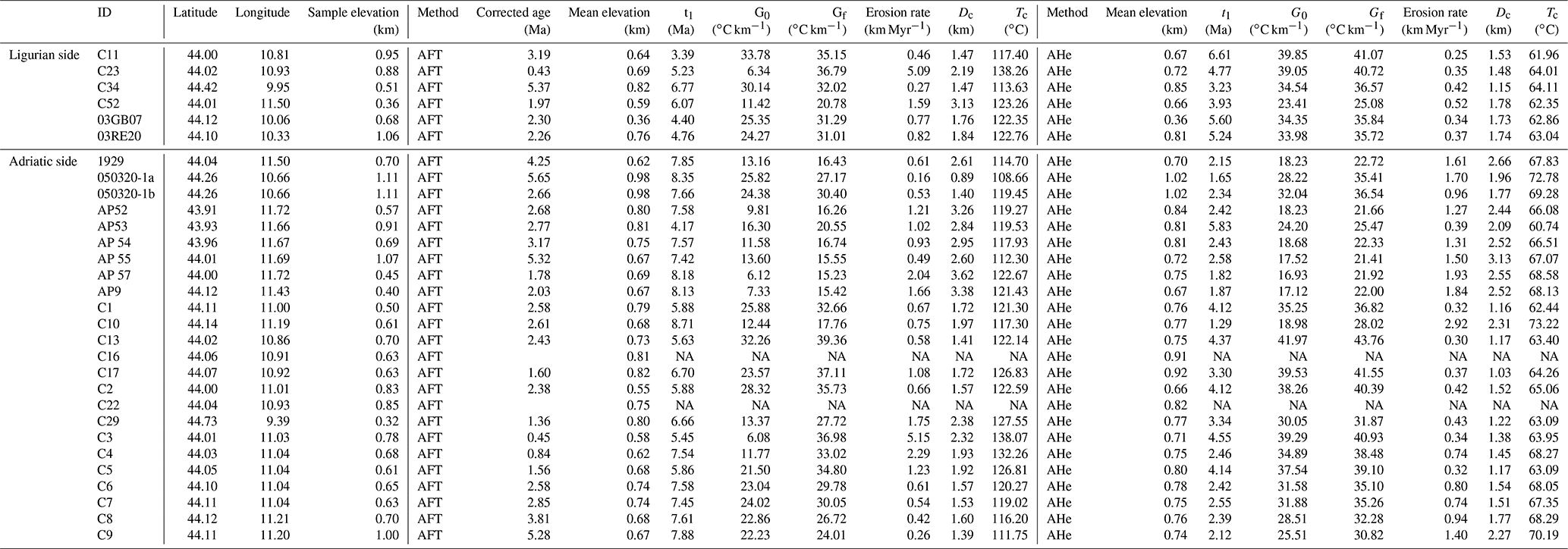
NA refers to not available.
3.3 Paired ages
Of the 30 paired samples analysed here, erosion rates for two samples could not be resolved (Table 4) due to the similarity in ages between the AFT and AHe thermochronometers (sample C16) or due to an AHe age that is older than the AFT age (sample C22). Six paired samples are located on the Ligurian side of the orogen, and the remaining 22 samples are located on the Adriatic side of the orogen (Fig. 9a).
Erosion rates from samples on the Adriatic side vary from ∼0.3 to 5.2 km Myr−1 (Table 4). In total, 12 samples illustrate an increase in erosion through time (Fig. 9b), with the shift generally occurring between ∼1 and 2 Ma. The 10 samples from the Adriatic side illustrate a decrease in erosion rate through time (Fig. 9c), with the shift generally occurring between ∼2 and 4 Ma. With the exception of three samples (AP53, AP57, and C29), decelerating sites are located in the headwaters of the Reno River (inset map, Fig. 9a), which drains the Cervarola and Macigno units east of Mt. Cimone (Fig. 1). For the six paired samples from the Ligurian side, the range of erosion rates is similar and varies from ∼0.3 to 5.1 km Myr−1 (Table 4). However, only one sample on the Ligurian side illustrates an increase in erosion rate, occurring at ∼3 Ma (Fig. 9d). All other samples illustrate a decrease in erosion through time, with the shift occurring between ∼6 and 2 Ma (Fig. 9e).
3.4 Kinematic model
The orogenic wedge model shows how the spatial pattern of exhumation rates relates to the polarity of accretion and the pattern of horizontal and vertical motion. Figure 10 illustrates the predicted horizontal velocities, uplift rates, and material paths through the wedge for the spatially constant erosion rate setup (SCR) and the spatially variable erosion rate (VER) setup. Horizontal velocities at the toes of the wedge are equal to the rate of slab rollback and decrease to a minimum at the drainage divide between the prowedge and retrowedge (Fig. 10a). Extension in the retrowedge results in higher horizontal erosion rates towards the Ligurian coast.
To construct the best-fit model, our goal is to reproduce the pattern of reset and non-reset thermochronometer ages and uplift rates from geodetic re-levelling (D'Anastasio et al., 2006) for the prowedge (0.5–1 km Myr−1) and retrowedge (−0.15–0.12 km Myr−1). To this end, we adjust the slab rollback rate within the acceptable range for our field area (6–20 km Ma−1), and the AHe erosion rates within the range of values calculated from Gf_heatflow (0.17–1.9 km Myr−1) (Table S5). Since ZHe samples are only reset near the Apuan Alps, an acceptable model should have ZHe cooling ages that are >10 Ma across the orogenic wedge, whereas AFT and AHe samples should be reset across the wedge. Increasing the erosion rates within the kinematic model produces younger cooling ages. Increasing the rate of slab rollback increases the horizontal component of motion for rock particles and produces particle paths with shallower maximum burial depths.
For the SCR setup, we ran the model with a single, orogen-wide erosion rate varying between 0.17 and 1.9 km Myr−1, which are values consistent with the range of AHe-derived erosion rates for the Adriatic side of the orogen. The best-fit model for the SCR scenario incorporates an orogen-wide erosion rate ( km Ma−1 and a slab rollback rate (VP)=9 km Myr−1. In this scenario, horizontal velocities decrease to a minimum of 2.8 km Myr−1 at the drainage divide (Fig. 10a). Uplift rates on the prowedge vary from 0.49 to 0.7 km Myr−1, and from 0 to 0.26 km Myr−1 on the retrowedge (Fig. 10b). Predicted reset cooling ages across the orogen for AHe samples (triangles) vary from 4.0 to 5.9 Ma, from 5.9 to 9.6 Ma for AFT samples (diamonds), and from 9.1 to 12.9 Ma for ZHe samples (circles) (Fig. 11a, c). Maximum burial depth increases almost linearly across the orogenic wedge, ranging from 1.9 to 2.7 km on the prowedge and from 3.2 to 6.0 km on the retrowedge (Fig. 11b).
For the VER setup, we prescribed a slab rollback rate (VP)=10 km Myr−1, a prowedge erosion rate (ep=0.6 km Myr−1), and a retrowedge erosion rate (er=0.3 km Myr−1). Horizontal velocities decrease to a minimum of 2.9 km Myr−1 at the drainage divide (Fig. 10d). Predicted uplift rates on the prowedge are 0.70–0.93 km Myr−1, and uplift rates on the retrowedge are −0.20–0.15 km Myr−1 (Fig. 10e). Predicted reset cooling ages range from 3.5 to 5.5 Ma for AHe samples, from 5.6 to 7.6 Ma for AFT samples, and from 10.8 to 11.6 Ma for ZHe samples. For samples that reach the surface on the prowedge side of the range, predicted reset cooling ages decrease towards the primary drainage divide. On the retrowedge, ages initially increase away from the divide but young slightly at the model boundary (Fig. 11d). Maximum burial depth for reset particles increases almost linearly along the prowedge (2.0–4.1 km) up to a kink at the drainage divide, which reflects the shift towards a shallower slope, where maximum burial depths along the retrowedge range from 4.6 to 6.8 km (Fig. 11e).
4.1 Detrital versus bedrock ages
Previous studies place the onset of exhumation between 8 and 14 Ma (Balestrieri et al., 1996; Ventura et al., 2001), so it is not clear whether the 12–13 Ma old population in the Vara and Magra samples represent partially or completely reset cooling ages. However, these ages are consistent with high-elevation samples west of the Vara catchment that record slow cooling prior to 8 Ma. The 8.2 Ma age peak is present in the Magra1 sample, which drains the extensional intermontane basin within the catchment, but is absent in the Magra2 sample, which drains only small tributaries upstream of the basin (Fig. 3b). Thus, the peak at 8.2 Ma in Magra1 likely reflects exhumation ages of the nearby Macigno Unit, which would have been eroded and redeposited into the Pliocene basins (Balestrieri, 2000; Fellin et al., 2007). The pulse of exhumation in the Northern Apennines between 6 and 4 Ma, when most of the Northern Apennines became sub-aerially exposed (Zattin et al., 2002; Balestrieri et al., 2003; Fellin et al., 2007), is consistent with the youngest peaks shown in the Vara, Magra, Lima, and Bisenzio rivers.
The pattern of detrital AFT ages on the Ligurian and Adriatic sides (Malusà and Balestrieri, 2012) is consistent with the pattern of bedrock AFT ages, which illustrate younging exhumation ages towards the NE, regardless of whether cooling ages are corrected or uncorrected for topography (Fig. 2). Overall, we find consistent results between the detrital AFT and bedrock AFT ages, reinforcing that the reset detrital ages illustrate a true exhumation signal, rather than an artefact of the technique. Fertility analysis of sediment from sampled Adriatic catchments also confirms that the detrital samples are representative of the eroded bedrock (Malusà et al., 2016a), in the absence of hydraulic sorting effects. Since the Ligurian catchments sampled in this study generally expose the same lithologies as the Adriatic catchments studied by Malusà et al. (2016a), this suggests that detrital samples on the Ligurian side are also representative of eroded bedrock.
4.2 Inferred erosion rate and relationship to the geothermal gradient
One of the parameters specified for the AGE2EDOT inversion is the onset time for erosion. An erosional unconformity (ca. 18 Ma) is recorded in the epi-Ligurian deposits, which has been attributed to a phase of major thrusting and sea level oscillations (Papani et al., 1987). This unconformity is succeeded by shelf deposits that record an overall shallowing trend in the epi-Ligurian basins and is thus not related to the emergence of the entire Apennine wedge, which is the time period in Apenninic history that we are modelling. In fact, stratigraphic and petrographic data indicate that the Northern Apennines increasingly provided detrital sediment to the foredeep through the middle–late Miocene, while the wedge was still submerged (Valloni et al., 2002). The first important clastic supply from the Northern Apennines dates to the Serravallian at ∼12 Ma (Caprara et al., 1985). Thus, in our erosion rate analysis, we used an onset time of 10 Ma as a reflection of the onset of heat advection due to erosion.
In the Northern Apennines, an erosion onset age of 10 Ma for the erosion rate analysis is a reasonable assumption for all samples from Cenozoic foredeep units with depositional ages far older than 10 Ma. For the Cenozoic foredeep units that were deposited in the middle–late Miocene, this assumption may not hold. Among the dated rocks compiled here, the youngest ones are the foredeep sediments of the Marnoso–Arenacea Unit, which has a depositional age as young as late Miocene. However, in most cases, reset ages from the Marnoso–Arenacea Unit are from areas that have depositional ages significantly older than 10 Ma. Given that accretion in the Northern Apennines occurs very shortly after deposition (e.g. Zattin et al., 2002), it is likely that accretion and erosion started close to 10 Ma, even for the youngest reset Marnoso–Arenacea samples. Assuming a later onset of erosion, for instance 8 Ma, would result in a slightly higher erosion rate. Finally, we note that using an erosion onset age of 14 Ma would not change the pattern of exhumation but would proportionally decrease all erosion rates in the Northern Apennines in response to a longer period of erosion. With regard to the detrital AFT samples, as we incorporate only the youngest population age from each sample, the 13 Ma age population of samples 1 to 3 would have no effect on the erosion rate calculations, even if we used an erosion onset at 14 Ma.
The geothermal gradient is the most important external parameter for converting cooling ages into erosion rates (Willett and Brandon, 2013). The two major studies of regional heat flow (della Vedova et al., 2001 and Pauselli et al., 2019) show large variations in heat flow across the region but are also internally inconsistent by up to 50 mW m−2 in the regions where they overlap. It is thus unclear how much of the spatial variability is real or how much is due to local effects or local errors in heat flow measurements, a large source of uncertainty for the geothermal gradients and, ultimately, the erosion rates. To address this uncertainty, we took two approaches. First, we assumed that the initial geothermal gradient in the region was uniform and all variations in the modern geothermal gradient are due to advection in response to erosion. Second, we constrained the thermal model to be consistent with the modern heat flow measurements and inferred an initial geothermal gradient that was spatially variable.
The uncertainties in the modern heat flow measurements are evident in the erosion rate analysis, particularly when comparing the range of G0_heatflow inferred from Gf_heatflow inputs that are calculated with heat flow measurements (Fig. 6a, d). However, it is unclear whether the large range of G0_heatflow values represents how the geothermal gradient may have varied in either space or time at the onset of erosion. As the Northern Apennines evolved, sediments were accreted to the accretionary wedge shortly after being deposited in a subsiding foreland basin, whose modern equivalents are the Po Plain and the Adriatic Sea. There, modern heat flow values are generally low (≤50 mW m−2) (della Vedova et al., 2001), although with significant spatial variations (Pauselli et al., 2019), indicating that the present geothermal gradients in the foreland should be not higher than about 30 ∘C km−1. Given the uncertainties in the modern heat flow measurements, the erosion analysis approach based on a common G0_25 can be considered a viable alternative to the approach based on an input Gf_heatflow.
The erosion rates resulting from these two analyses differ significantly: erosion rates from one analysis are a factor of 2 different from the alternate analysis (Fig. 6). However, the two sets of results projected along swath profiles from SW to NE show little difference in their spatial patterns across the main Apenninic divide (Fig. 8). The main differences are that the erosion rates derived from Gf_heatflow vary over a larger and higher range than those derived from G0_25, and the maximum rates are higher from Gf_heatflow. In particular, the youngest detrital age populations give much larger rates on the Adriatic side than on the Ligurian side with the analysis based on Gf_heatflow. These observations suggest that the erosion rates derived from G0_25 may be more conservative estimates overall. However, the most important observation for the scope of this contribution remains that the large-scale spatial pattern of erosion rates along the swath profile does not change with the employed analysis method.
4.3 Erosion rate patterns
Bedrock cooling ages on the Ligurian side of the Northern Apennines generally vary between 4 and 10 Ma (Fig. 7a, b), with only a few ages younger than 4 Ma. On the Adriatic side, bedrock cooling ages younger than 4 Ma are a large component of the age distributions, especially among the AHe ages (Fig. 7d). Similarly, the youngest populations for detrital AFT samples on the Ligurian side are nearly all older than the youngest detrital AFT populations on the Adriatic side (Fig. 7a, c).
Erosion rates derived from both bedrock and detrital thermochronometric ages suggest a difference between the Ligurian and Adriatic sides that is valid at the regional scale, regardless of the method used for constraining the geothermal gradients. An exception to this general pattern may be the Apuan Alps massif, which represents a structural culmination exposing a deep section and where high exhumation rates from the latest Miocene to the present likely reflect post-orogenic processes of crustal thinning (Fellin et al., 2007; Molli et al., 2018). On the Ligurian side, erosion rates derived from bedrock AFT ages (Fig. 7e) tend to be higher than erosion rates obtained from bedrock AHe ages (Fig. 7f) reflecting a regional decrease in erosion rate. This is particularly evident in the region east of the Apuan Alps, at the main drainage divide north of Florence and in the Val d'Arno (Figs. 1 and 2). In contrast, on the Adriatic side, erosion rates derived from AHe ages (Fig. 7h) tend to be higher than erosion rates obtained from AFT ages (Fig. 7g) and suggest an increase in erosion rate over the last 5 Myr.
Paired thermochronometers on the same sample (as, for instance, AFT and AHe) or AETs also indicate temporal changes in erosion rate. The majority of the paired-age samples (12) from the Adriatic side illustrate an increase in erosion rate through time (Fig. 9b), although 10 of these samples illustrate a decrease in erosion through time (Fig. 9c). Of these 10 samples, 7 are from one region of the upper Reno River Valley (Fig. 9a). The headwaters of the Reno River Valley extend farther south than the adjacent basins of the Serchio River and Bisenzio River, which flow to the Ligurian Sea (Fig. 3a). Interestingly, the exhumation rates from the upper Reno River are similar to rates from the Serchio River, suggesting that the upper Reno River presents an erosion rate signal akin to Ligurian rivers, rather than to Adriatic rivers, and are thus resolving a consistent pattern of erosion rate in space, but not restricted to catchment boundaries. We also note that modern erosion rates from cosmogenic nuclide concentrations in the upper Reno tributaries are at least a factor of 3 lower than rates for the entire basin (Cyr et al., 2010), suggesting that the trend of lower erosion rates in this area has continued to the present.
Paired ages from the Ligurian side show the opposite trend. With the exception of one sample (C34) (Fig. 9d) located within the Magra2 catchment area (Fig. 3a), all other samples consistently illustrate a decrease in erosion rate through time (Fig. 9e). Thus, the results from the paired thermochronometer ages on the Adriatic and Ligurian sides of the orogen confirm the regional trends observed from the simple erosion rate analysis method.
The results from our paired-age analysis can also be discussed in the context of the AETs from Mt. Falterona, Mt. Cimone, and Val d'Arno (see Fig. 1 for locations). Between 4 and 2 Ma, these AETs have previously been interpreted to reflect an orogen-wide increase in exhumation and erosion rates, although there are notable differences between the results from the profiles on the Adriatic side (Mt. Falterona and Mt. Cimone) and on the Ligurian side (Val d'Arno) (Thomson et al., 2010). The Mt. Falterona and Cimone AETs illustrate a 2-fold increase in erosion rates between 4 and 5 Ma, from 0.29 ± 0.1 to 0.58 ± 0.23 km Myr−1 and from 0.22 ± 0.09 to 0.58 ± 0.16 km Myr−1, respectively (Thomson et al., 2010). Excluding the samples from the upper Reno River Valley that illustrate a decrease in erosion rate through time, our paired-age analysis reflects erosion rates that increase from 0.68 ± 0.42 to 1.31 ± 0.70 km Myr−1, given 1σ uncertainties. Our average erosion rates are higher than the average erosion rates calculated for the Mt. Falterona and Cimone AETs, although, given the high uncertainties in our values, they are within the range of the AETs.
The results from the Val d'Arno AET are less straightforward, due to the fact that some samples illustrate a decrease in erosion rate through time, while others illustrate an increase in erosion rate through time. When corrected for topographic and advection effects, this AET shows a negative slope that was previously interpreted to reflect post-cooling tilting of the footwall block of an extensional fault (Thomson et al., 2010). On the Ligurian side, cooling ages and erosion rates vary locally as a function of elevation and of fault activity, and extensional faults can control differences in the exhumation pattern. However, in light of our results from the simple analysis of erosion rates and the paired ages, this negative slope could also be interpreted as a decrease in erosion rates and thus would reflect a regional signal rather than local tectonics. We infer that such regional-scale differences must be controlled by first-order features of the Northern Apennines. In order to address the question of what could control such differences, we compare two different kinematic models for the Northern Apennine orogenic wedge.
4.4 Kinematic model
The orogenic wedge kinematic models illustrate differences in cooling ages, maximum burial temperatures, and material paths across the Northern Apennine wedge, assuming simple continuum accretion and mass balance (Fig. 11). Since we constrain the range of possible prowedge and retrowedge erosional velocities from AHe erosion rates, the kinematic model can be assumed to reflect the more recent <5 Ma evolution of the Northern Apennines, when the Northern Apennines experienced major uplift and erosional exhumation (i.e. early Pliocene). Using a spatially constant erosion rate across the orogenic wedge (SCR) predicts that reset ages decrease from northeast to southwest and are youngest on the retrowedge model boundary. While this pattern is consistent with observed ZHe ages that are reset only near the Ligurian coastline, the SCR model cannot recreate the pattern of older observed AFT and AHe cooling ages on the retrowedge (Fig. 7a–d). In contrast, the VER setup predicts minimum reset ages near the drainage divide and maximum reset ages on the retrowedge, close to the model boundary. The VER model does not predict any ZHe reset ages, although the pattern of predicted AFT and AHe cooling ages is consistent with the pattern of observed cooling ages, which are youngest near the drainage divide in the core of the Northern Apennines (Fig. 2).
Slab rollback rates vary over an order of magnitude in the Northern Apennines (6–20 km Myr−1). Higher values of slab rollback can reproduce the pattern of cooling ages across the Northern Apennines, although predicted maximum burial depths decrease with higher slab rollback rates. Vitrinite reflectance (VR) data provide an additional estimate for maximum palaeotemperatures and burial depth and thus, an additional calibration of the kinematic model. In the Northern Apennines, Ro values reach 5.1 % at the Ligurian coastline along the Mt. Gottero swath profile (Fig. 2a). With the exception of this profile, maximum VR values are generally within the range of 1.5 %–2.5 % for the Mt. Cimone, Bologna, and Val d'Arno profiles (Fig. 2b, d). Maximum palaeotemperatures from VR are estimated at 200–250 ∘C in the core of the range and along the Ligurian coastline in the northwest (Fellin et al., 2007), whereas palaeotemperatures are 150–190 ∘C in the Cervarola Unit (VR of 1.0–1.7 %) and 100–110 ∘C in the Ligurian Unit (VR of 0.5–0.6 %) (Ventura et al., 2001; Botti et al., 2004). Maximum palaeotemperatures should correspond to maximum burial depths; thus, we expect to find the maximum burial depths along the Ligurian coastline and near the drainage divide in the Cervarola Unit. Both the SCR and VER models predict maximum burial depths near the Ligurian coastline, consistent with the trends observed in the Mt. Gottero and Val d'Arno profile. Near the drainage divide on the prowedge, predicted maximum burial depths are 2.9 km for the SCR model and 4.1 km for the VER model.
We can estimate maximum burial depths at the drainage divide, given the generalized relationship between Ro and burial depth (Suggate, 1998), VR values, and a modern geothermal gradient. To estimate the modern geothermal gradient at the drainage divide, we use Gf_heatflow rates from the simple erosion analysis for AHe samples in the Cervarola Unit (Table S5). Given these parameters, we estimate maximum burial depths in the range of 4.0–5.5 km near the drainage divide, consistent with the predicted maximum burial depth for the VER model. Collectively, our erosion rate analysis and kinematic model illustrate that the east-to-west particle trajectories, combined with lower erosion rates on the retrowedge by a factor of 2, are consistent with the spatial pattern of cooling ages and maximum palaeotemperatures estimated from both vitrinite reflectance and thermochronometric data.
The particle paths in the VER kinematic model, combined with the lower erosion rates in the retrowedge, suggest an explanation for the apparent decrease in erosion rates with time on the Ligurian side of the Apennines. As rocks are advected from prowedge to retrowedge, the vertical component of their motion decreases (Fig. 10f). Particle paths where the AFT cooling age is set in the prowedge, but where the AHe cooling age is set in the retrowedge, will record this change as a temporal deceleration of cooling rate. However, rather than representing a change in surface erosion rate, the change in cooling rate reflects the motion of the rock from the fast erosion rate prowedge into the low erosion rate retrowedge. The fact that the decelerating sites are all found to the southwest, regardless of drainage basin (inset, Fig. 8c), supports the idea that this is a tectonically controlled spatial pattern.
The acceleration of exhumation observed in the prowedge is not explained by the kinematic model. The acceleration of exhumation may be related to a change in the timing or rate of slab rollback, which has varied along strike and across the orogen (Faccenna et al., 2014; Rosenbaum and Piana Agostinetti, 2015) and is a first-order tectonic control on exhumation and erosion (Thomson et al., 2010). We allow for a range of rollback rates that are consistent with rates for the field area, although the kinematic model is not able to resolve variability in rollback rates in either space or time, nor can it resolve how rotation or motion external to the wedge (e.g. lateral translation of the Adriatic slab relative to the Apennine wedge) would alter the flux or orientation of material entering the wedge. Alternatively, the apparent increase in exhumation rate might be explained by spatial changes in tectonic uplift and an associated increase in erosion rate, although there is no strong evidence for this in the spatial pattern of ages or in the geomorphology, which should show higher uplift rates in the range interior. In contrast, the highest uplift rates are more often observed at the mountain front (Picotti and Pazzaglia, 2008). It is more likely that this is a true temporal increase in erosion rate, which could be associated with an increase in accretionary flux as the mountain front advanced into the Alpine sediments of the Adriatic foreland. The foreland basin fill thickened as Miocene alpine sediments filled the foredeep and again in the Quaternary as glacial sediments filled the Po Plain and parts of the Adriatic Sea. The increase in accretionary flux would lead to an increase in wedge size and in erosion rate, processes that our kinematic model does not include. The increase in erosion rate could also be associated with a direct, externally driven increase in surface erosion rate associated with Quaternary climate change. Although the Apennines were not significantly affected by alpine glaciation, the cooling and strong cyclicity of the Quaternary climate may have led to an increase in erosion rate through the efficiency of periglacial processes and hillslope processes such as landsliding (Amorosi et al., 1996; Borgatti and Soldati, 2010; Simoni et al., 2013; Wegmann and Pazzaglia, 2009).
We present evidence from multiple thermochronometers that the spatial and temporal patterns of erosion rates in the Northern Apennine orogen differ at the regional scale. New detrital AFT cooling ages from the Ligurian side of the orogen are similar to AFT bedrock cooling ages from the Ligurian side, illustrating that the detrital ages reflect a true exhumation signal across the Northern Apennines. Time-averaged erosion rates from individual thermochronometers predict faster erosion rates derived from AHe ages on the Adriatic side relative to the Ligurian side. These results are consistent with erosion rates derived from paired AFT–AHe thermochronometer samples, which illustrate an increase in erosion rates through time on the Adriatic side, but a decrease in erosion rates through time on the Ligurian side. The pattern of erosion rates, observed maximum burial depths, and modern uplift rates across the orogen can be replicated with a kinematic model for an asymmetric orogen that includes both frontal accretion and underplating modes of crustal accretion, a slab rollback rate of 10 km Myr−1, and prowedge erosion rates that are a factor of 2 higher than retrowedge erosion rates. This model suggests that observed decelerations on the retrowedge are the result of the spatial advection of rock to the SW, although the observed acceleration of erosion rates on the prowedge requires external forcing, either through an increase in accretionary flux or through more erosive conditions linked to climate change.
All data used in this study are included in the text. Related codes for the erosion rate analysis and kinematic model are available upon request to the corresponding author.
The supplement related to this article is available online at: https://doi.org/10.5194/se-13-347-2022-supplement.
EDE, MGF, and SDW collected the detrital AFT samples in Northern Apennine catchments. EDE and MGF processed and analysed the detrital AFT samples. SDW wrote the kinematic model. EDE, MGF, and SDW all contributed to the interpretation of the data. EDE wrote the manuscript and created the figures with input from MGF and SDW.
The contact author has declared that neither they nor their co-authors have any competing interests.
Publisher’s note: Copernicus Publications remains neutral with regard to jurisdictional claims in published maps and institutional affiliations.
We thank two anonymous reviewers and the editor, whose input greatly improved our study.
This research has been supported by the Schweizerischer Nationalfonds zur Förderung der Wissenschaftlichen Forschung (grant no. SINERGIA Swiss Alp Array project (SNF no. 154434)).
This paper was edited by Federico Rossetti and reviewed by two anonymous referees.
Abbate, E., Balestrieri, M. L., Bigazzi, G., Norelli, P., and Quercioli, C.: Fission track datings and recent rapid denudation in Northern Apennines, Mem. Soc. Geol. It, 48, 579–585, 1994.
Abbate, E., Balestrieri, M. L., Bigazzi, G., Ventura, B., Zattin, M., and Zuffa, G. G.: An extensive apatite fission-track study throughout the Northern Apennines Nappe belt, Radiat. Meas., 31, 673–676, https://doi.org/10.1016/S1350-4487(99)00168-7, 1999.
Amorosi, A., Farina, M., Severi, P., Preti, D., Caporale, L., and Di Dio, G.: Genetically related alluvial deposits across active fault zones: An example of alluvial fan-terrace correlation from the upper Quaternary of the southern Po Basin, Italy, Sediment. Geol., 102, 275–295, https://doi.org/10.1016/0037-0738(95)00074-7, 1996.
Argnani, A. and Lucchi, F. R.: Tertiary silicoclastic turbidite systems of the Northern Apennines, in Anatomy of an orogen: the Apennines and adjacent Mediterranean basins, Springer, 327–349, 2001.
Balestrieri, M. L.: Exhumation ages and block faulting on the eastern flank of the Serchio graben (northern Apennines), in: 9th International Conference on Fission Track Dating and Thermochronology, Victoria, Australia, 6–11 February 2000, Geological Society of Australia Abstract Series, 58, 11–12, 2000.
Balestrieri, M. L., Abbate, E., and Bigazzi, G.: Insights on the thermal evolution of the Ligurian Apennines (Italy) through fission-track analysis, J. Geol. Soc. Lond., 153, 419–425, https://doi.org/10.1144/gsjgs.153.3.0419, 1996.
Balestrieri, M. L., Bernet, M., Brandon, M. T., Picotti, V., and Reiners, P. W., and Zattin, M.: Pliocene and Pleistocene exhumation and uplift of two key areas of the Northern Apennines, Quat. Int., 101, 67–73, 2003.
Balestrieri, M. L., Benvenuti, M., and Catanzariti, R.: Unravelling basin shoulder dynamics through detrital apatite fission-track signature: the case of the Quaternary Mugello Basin, Italy, Geol. Mag., 155, 1413–1426, https://doi.org/10.1017/s0016756817000073, 2018.
Bertoldi, R.: Una sequenza palinologica di età rusciniana nei sedimenti lacustri basali del bacino di Aulla-Olivola (Val di Magra), Riv. Ital. Paleontol. Stratigr., 94, 105–138, 1988.
Bonini, M., Moratti, G., Sani, F., and Balestrieri, M. L.: Compression-to-extension record in the late pliocene-pleistocene upper valdarno basin (Northern Apennines, Italy): Structural and thermochronological constraints, Ital. J. Geosci., 132, 54–80, https://doi.org/10.3301/IJG.2011.18, 2013.
Borgatti, L. and Soldati, M.: Landslides as a geomorphological proxy for climate change: A record from the Dolomites (northern Italy), Geomorphology, 120, 56–64, https://doi.org/10.1016/j.geomorph.2009.09.015, 2010.
Botti, F., Aldega, L., and Corrado, S.: Sedimentary and tectonic burial evolution of the Northern apennines in the modena-bologna area: Constraints from combined stratigraphic, structural, organic matter and clay mineral data of Neogene thrust-top basins, Geodin. Acta, 17, 185–203, https://doi.org/10.3166/ga.17.185-203, 2004.
Brandon, M. T.: Decomposition of mixed grain age distributions using Binomfit, On Track, 24, 13–18, 2002.
Caprara, L., Garzanti, E., Gnaccolini, M., and Mutt, L.: Shelf-basin transition: sedimentology and petrology of the Serravallian of the Tertiary Piedmont Basin (Northern Italy), Riv. Ital. Paleontol. Stratigr., 90, 1985.
Carlini, M., Artoni, A., Aldega, L., Balestrieri, M. L., Corrado, S., Vescovi, P., Bernini, M., and Torelli, L.: Exhumation and reshaping of far-travelled/allochthonous tectonic units in mountain belts. New insights for the relationships between shortening and coeval extension in the western Northern Apennines (Italy), Tectonophysics, 608, 267–287, https://doi.org/10.1016/j.tecto.2013.09.029, 2013.
Cibin, U., Spadafora, E., Zuffa, G. G., and Castellarin, A.: Continental collision history from arenites of episutural basins in the Northern Apennines, Italy, Bull. Geol. Soc. Am., 113, 4–19, https://doi.org/10.1130/0016-7606(2001)113< 0004:CCHFAO>2.0.CO;2, 2001.
Cita Sironi, M. B., Abbate, E., Balini, M., Conti, M. A., Germani, D., Groppelli, G., Manetti, P., and Petti, M. N.: Catalogo delle formazioni. Unità tradizionali, Cart. Geol. d'Italia, 1, 2006.
Cyr, A. J., Granger, D. E., Olivetti, V., and Molin, P.: Quantifying rock uplift rates using channel steepness and cosmogenic nuclide-determined erosion rates: Examples from northern and southern Italy, Lithosphere, 2, 188–198, https://doi.org/10.1130/L96.1, 2010.
D'Anastasio, E., De Martini, P. M., Selvaggi, G., Pantosti, D., Marchioni, A., and Maseroli, R.: Short-term vertical velocity field in the Apennines (Italy) revealed by geodetic levelling data, Tectonophysics, 418, 219–234, https://doi.org/10.1016/j.tecto.2006.02.008, 2006.
Delfrati, L., Falorni, P., Gropelli, G., and Petti, F. M.: Catalogo delle formazioni-Unità tradizionali, Quaderni serie III, Vol 7, fasciolo III, Cart. Geol. d'Italia, 1, 2002.
Faccenna, C., Becker, T. W., Miller, M. S., Serpelloni, E., and Willett, S. D.: Isostasy, dynamic topography, and the elevation of the Apennines of Italy, Earth Planet. Sc. Lett., 407, 163–174, https://doi.org/10.1016/j.epsl.2014.09.027, 2014.
Farley, K. A.: Helium diffusion from apatite: General behavior as illustrated by Durango fluorapatite, J. Geophys. Res.-Sol. Ea., 105, 2903–2914, https://doi.org/10.1029/1999JB900348, 2000.
Fellin, M. G., Reiners, P. W., Brandon, M. T., Wüthrich, E., Balestrieri, M. L., and Molli, G.: Thermochronologic evidence for the exhumational history of the Alpi Apuane metamorphic core complex, northern Apennines, Italy, Tectonics, 26, 1–22, https://doi.org/10.1029/2006TC002085, 2007.
Galbraith, R. F.: On statistical models for fission track counts, J. Int. Assoc. Math. Geol., 13, 471–478, 1981.
Garzanti, E. and Malusà, M. G.: The Oligocene Alps: Domal unroofing and drainage development during early orogenic growth, Earth Planet. Sc. Lett., 268, 487–500, 2008.
Hurford, A. J.: Standardization of fission track dating calibration: Recommendation by the Fission Track Working Group of the IUGS Subcommission on Geochronology, Chem. Geol. Isot. Geosci. Sect., 80, 171–178, 1990.
Hurford, A. J. and Green, P. F.: The zeta age calibration of fission-track dating, Chem. Geol., 41, 285–317, 1983.
Lustrino, M., Morra, V., Fedele, L., and Franciosi, L.: Beginning of the Apennine subduction system in central western Mediterranean: Constraints from Cenozoic “orogenic” magmatic activity of Sardinia, Italy, Tectonics, 28, https://doi.org/10.1029/2008TC002419, 2009.
Malinverno, A. and Ryan, W. B. F.: Extension in the Tyrrhenian Sea and shortening in the Apennines as result of arc migration driven by sinking of the lithosphere, Tectonics, 5, 227–245, 1986.
Malusà, M. G. and Balestrieri, M. L.: Burial and exhumation across the Alps-Apennines junction zone constrained by fission-track analysis on modern river sands, Terra Nov., 24, 221–226, https://doi.org/10.1111/j.1365-3121.2011.01057.x, 2012.
Malusà, M. G., Faccenna, C., Baldwin, S. L., Fitzgerald, P. G., Rossetti, F., Balestrieri, M. L., Danišík, M., Ellero, A., Ottria, G., and Piromallo, C.: Contrasting styles of (U) HP rock exhumation along the Cenozoic Adria-Europe plate boundary (Western Alps, Calabria, Corsica), Geochem. Geophys. Geosys., 16, 1786–1824, 2015.
Malusà, M. G., Resentini, A., and Garzanti, E.: Hydraulic sorting and mineral fertility bias in detrital geochronology, Gondwana Res., 31, 1–19, https://doi.org/10.1016/j.gr.2015.09.002, 2016a.
Malusà, M. G., Anfinson, O. A., Dafov, L. N., and Stockli, D. F.: Tracking Adria indentation beneath the Alps by detrital zircon U-Pb geochronology: Implications for the Oligocene-Miocene dynamics of the Adriatic microplate, Geology, 44, 155–158, https://doi.org/10.1130/G37407.1, 2016b.
Merla, G.: Geologia dell'Appennino settentrionale, Arti Grafiche Pacini Mariotti, 1952.
Molli, G., Vitale Brovarone, A., Beyssac, O., and Cinquini, I.: RSCM thermometry in the Alpi Apuane (NW Tuscany, Italy): New constraints for the metamorphic and tectonic history of the inner northern Apennines, J. Struct. Geol., 113, 200–216, https://doi.org/10.1016/j.jsg.2018.05.020, 2018.
Ori, G. G. and Friend, P. F.: Sedimentary basins formed and carried piggyback on active thrust sheets., Geology, 12, 475–478, https://doi.org/10.1130/0091-7613(1984)12< 475:SBFACP>2.0.CO;2, 1984.
Papani, G., Tellini, C., Torelli, L., Vernia, L., and Iaccarino, S.: Nuovi dati stratigrafici e strutturali sulle formazione di Bismantova nella sinclinale Vetto-Carpineti (Appennino Reggiano-Parmense), Mem. Della Soc. Geol. Ital., 39, 245–275, 1987.
Pauselli, C., Gola, G., Mancinelli, P., Trumpy, E., Saccone, M., Manzella, A., and Ranalli, G.: A new surface heat flow map of the Northern Apennines between latitudes 42.5 and 44.5∘ N, Geothermics, 81, 39–52, https://doi.org/10.1016/j.geothermics.2019.04.002, 2019.
Pialli, G., Plesi, G., Damiani, A. V, Brozzetti, F., Boscherini, A., Bucefalo Palliani, R., Cardinali, M., Checcucci, R., Daniele, G., and Galli, M.: Note illustrative del Foglio 289 “Città di Castello”, Cart. Geol. d'Italia, 1, 2000.
Picotti, V. and Pazzaglia, F. J.: A new active tectonic model for the construction of the Northern Apennines mountain front near Bologna (Italy), J. Geophys. Res.-Sol. Ea., 113, 1–24, https://doi.org/10.1029/2007JB005307, 2008.
Pini, G. A.: Tectonosomes and Olistostromes in the Argile Scagliose of the Northern Apennines, Geol. Soc. Am. Spec. Pap., 335, 70, https://doi.org/10.1130/0-8137-2335-3.1, 1999.
Reiners, P. W. and Brandon, M. T.: Using Thermochronology To Understand Orogenic Erosion, Annu. Rev. Earth Planet. Sci., 34, 419–466, https://doi.org/10.1146/annurev.earth.34.031405.125202, 2006.
Reutter, K. J., Teichmüller, M., Teichmüller, R., and Zanzucchi, G.: The coalification pattern in the Northern Apennines and its palaeogeothermic and tectonic significance, Geol. Rundschau, 72, 861–893, https://doi.org/10.1007/BF01848346, 1983.
Ricci Lucchi, F.: The Oligocene to Recent foreland basins of the northern Appennines, edited by: Allen, A. and Homewood, P., Forel. Basins, 105–139, https://doi.org/10.1002/9781444303810.ch6, 1986.
Rosenbaum, G. and Piana Agostinetti, N.: Crustal and upper mantle responses to lithospheric segmentation in the northern Apennines, Tectonics, 34, 648–661, https://doi.org/10.1002/2013TC003498, 2015.
Simoni, A., Ponza, A., Picotti, V., Berti, M., and Dinelli, E.: Earthflow sediment production and Holocene sediment record in a large Apennine catchment, Geomorphology, 188, 42–53, https://doi.org/10.1016/j.geomorph.2012.12.006, 2013.
Spada, M., Bianchi, I., Kissling, E., Agostinetti, N. P., and Wiemer, S.: Combining controlled-source seismology and receiver function information to derive 3-D moho topography for italy, Geophys. J. Int., 194, 1050–1068, https://doi.org/10.1093/gji/ggt148, 2013.
Suggate, R. P.: Relations between depth of burial, vitrinite reflectance and geothermal gradient, J. Pet. Geol., 22, 5–32, https://doi.org/10.1111/j.1747-5457.1999.tb00471.x, 1998.
Thomson, S. N., Brandon, M. T., Reiners, P. W., Zattin, M., and Isaacson, P. J. and Balestrieri, M. L.: Thermochronologic evidence for orogen-parallel variability in wedge kinematics during extending convergent orogenesis of the northern Apennines, Italy, Bull. Geol. Soc. Am., 122, 1160–1179, https://doi.org/10.1130/B26573.1, 2010.
Vai, F. and Martini, I. P.: Anatomy of an orogen: the Apennines and adjacent Mediterranean basins, Springer, ISBN 978-90-481-4020-6, 2001.
Valloni, R., Cipriani, N., and Morelli, C.: Petrostratigraphic record of the Apennine foredeep basins, Italy, Boll. Della Soc. Geol. Ital., 121, 455–465, 2002.
della Vedova, B., Bellani, S., Pellis, G., and Squarci, P.: Heat Flow Distribution, in: Anatomy of an orogen: the Apennines and adjacent Mediterranean basins, edited by: Vai, G. B. and Martini, I. P., 65–76, 2001.
Ventura, B., Pini, G. A., and Zuffa, G. G.: Thermal history and exhumation of the Northern Apennines (Italy): evidence from combined apatitefissio-track and vitrinite reflectance data from foreland basin sediments, Basin Res., 13, 435–448, https://doi.org/10.1046/j.0950-091X.2001.00159.x, 2001.
Wagner, G. A. and Van Den Haute, P.: Fission-Track Dating, Kluwer Academic Publishers, Dordrecht, Netherlands, ISBN 978-94-010-5093-7, 1992.
Wegmann, K. W. and Pazzaglia, F. J.: Late Quaternary fluvial terraces of the Romagna and Marche Apennines, Italy: Climatic, lithologic, and tectonic controls on terrace genesis in an active orogen, Quat. Sci. Rev., 28, 137–165, https://doi.org/10.1016/j.quascirev.2008.10.006, 2009.
Willett, S. D. and Brandon, M. T.: Some analytical methods for converting thermochronometric age to erosion rate, [code], Geochem., Geophys. Geosys., 14, 209–222, https://doi.org/10.1029/2012GC004279, 2013.
Willett, S. D., Slingerland, R., and Hovius, N.: Uplift, shortenning, and steady state topography in active mountain belts, Am. J. Sci., 301, 455–485, 2001.
Willett, S. D., Herman, F., Fox, M., Stalder, N., Ehlers, T. A., Jiao, R., and Yang, R.: Bias and error in modelling thermochronometric data: Resolving a potential increase in Plio-Pleistocene erosion rate, Earth Surf. Dyn., 9, 1153–1221, 2021.
Wilson, L. F., Pazzaglia, F. J. and Anastasio, D. J.: A Fluvial record of active fault-propagation folding, salsomaggiore anticline, northern Apennines, Italy, J. Geophys. Res.-Sol. Ea., 114, 1–23, https://doi.org/10.1029/2008JB005984, 2009.
Zattin, M., Picotti, V. and Zuffa, G. G.: Fission-track reconstruction of the front of the Northern Apennine thrust wedge and overlying Ligurian unit, Am. J. Sci., 302(4), 346–379, https://doi.org/10.2475/ajs.302.4.346, 2002.