the Creative Commons Attribution 4.0 License.
the Creative Commons Attribution 4.0 License.
 | 21 Feb 2022
Reflection tomography by depth warping: a case study across the Java trench
Dirk Klaeschen
Heidrun Kopp
Michael Schnabel
Accurate subsurface velocity models are crucial for geological interpretations based on seismic depth images. Seismic reflection tomography is an effective iterative method to update and refine a preliminary velocity model for depth imaging. Based on residual move-out analysis of reflectors in common image point gathers, an update of the velocity is estimated by a ray-based tomography. To stabilize the tomography, several preconditioning strategies exist. Most critical is the estimation of the depth error to account for the residual move-out of the reflector in the common image point gathers. Because the depth errors for many closely spaced image gathers must be picked, manual picking is extremely time-consuming, human biased, and not reproducible. Data-driven picking algorithms based on coherence or semblance analysis are widely used for hyperbolic or linear events. However, for complex-shaped depth events, purely data-driven picking is difficult. To overcome this, the warping method named non-rigid matching is used to estimate a depth error displacement field. Warping is used, for example, to merge photographic images or to match two seismic images from time-lapse data. By matching a common image point gather against its duplicate that has been shifted by one offset position, a locally smooth-shaped displacement field is calculated for each data sample by gather matching. Depending on the complexity of the subsurface, sample tracking through the displacement field along predefined horizons or on a simple regular grid yields discrete depth error values for the tomography. The application to a multi-channel seismic line across the Sunda subduction zone offshore Lombok island, Indonesia, illustrates the approach and documents the advantages of the method to estimate a detailed velocity structure in a complex tectonic regime. By incorporating the warping scheme into the reflection tomography, we demonstrate an increase in the velocity resolution and precision by improving the data-driven accuracy of depth error picks with arbitrary shapes. This approach offers the possibility to use the full capacities of tomography and further leads to more accurate interpretations of complex geological structures.
- Article
(33635 KB) - Full-text XML
- BibTeX
- EndNote


Reflection tomography and pre-stack depth migration of multi-channel seismic reflection (MCS) data have evolved into standard seismic data processing routines in recent decades, owing to the rapid development of CPU performance and the effective adaption of seismic data processing software. Pre-stack depth migration (PSDM) of near-vertical reflections is the algorithm of choice in reflection seismology to properly image steeply dipping reflectors while accounting for non-hyperbolic move-out caused by lateral velocity variations (Yilmaz, 2001; Jones et al., 2008) and thus is applied in tectonically and structurally complex geological settings in 2-D and 3-D migration strategies (Collot et al., 2011; Han et al., 2017; Li et al., 2018; Shiraishi et al., 2019). However, the quality of subsurface imaging depends on the seismic velocity model that is used for the migration. An exact determination of the velocity field is thus crucial to retrieve an optimal subsurface image.
The velocity field may be determined during PSDM by performing velocity analysis on selected locations using depth-focusing error analysis (Audebert and Diet, 2008; MacKay and Abma, 1992) or hyperbolic residual move-out (RMO) correction of common image point (CIP) gathers followed by a simple vertical Dix inversion (Dix, 1955) at each location independently. Thus a structural velocity model (Audebert et al., 1997) may be built manually by defining depth horizons. Manual picking or pre-definition of depth horizons, however, are not only time-consuming for seismic processors but, more importantly, may also lead to a subjective interpretation bias (Jones, 2003).
In contrast, the velocity model design based on reflection tomography inverts all CIP locations simultaneously to update the velocity structure and yields a more complete solution than manually designed velocity models (Bishop et al., 1985; Van Trier, 1990; Stork, 1992; Kosloff et al., 1996). While the Dix inversion strips off the layers from top to bottom in a flat-layer approach, the reflection tomography accounts for dipping layers and lateral velocity changes within the streamer length (Jones, 2010). The general procedure for reflection tomography is to go into the pre-stack migrated CIP offset domain and to measure the hyperbolic residual move-out of the depth misalignment (also called depth error) by manual picking or by automatic scanning techniques (Hardy, 2003; Claerbout, 1992). Subsequently, the depth error is inverted to velocity changes to flatten the reflector signals over the entire offset range (Jones et al., 2008; Fruehn et al., 2008; Riedel et al., 2019). For cases where the MCS data do not provide sufficient move-out sensitivity to estimate reliable velocities (i.e. deep target depth), several velocity inversion strategies have been established to combine near-vertical reflections, wide-angle (WA) reflections, and refracted events (Gras et al., 2019; Górszczyk et al., 2019; Melendez et al., 2019).
By relating changes of the CIP depth errors to changes in velocities along source–receiver rays in the direction normal to the local reflector dip, a new velocity can be calculated to minimize the CIP depth errors. To solve the general non-linear inverse tomographic problem, the velocity error is gauged iteratively, inverted, and updated as depicted by the loop in Fig. 1.
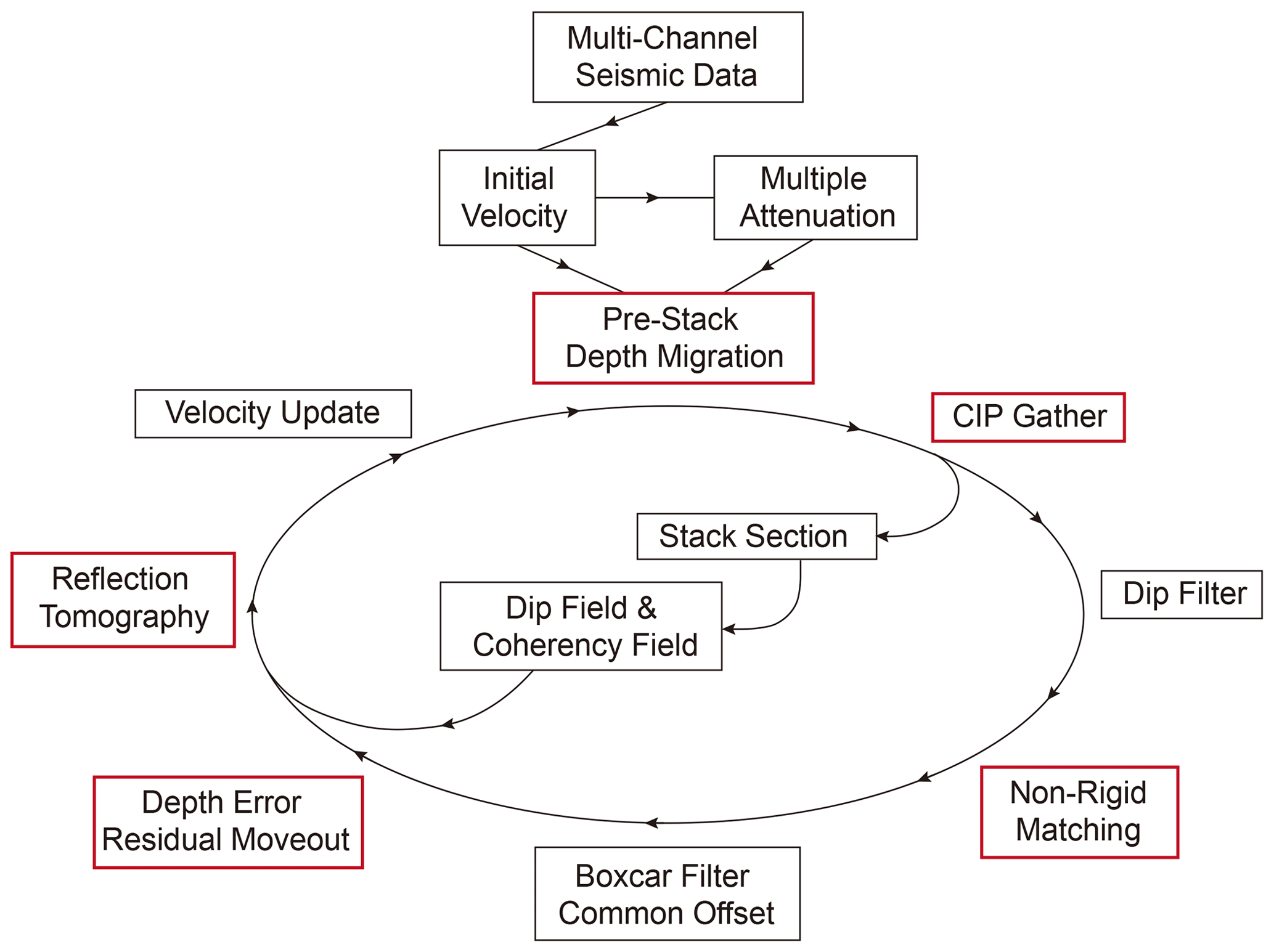
Figure 1Processing scheme using non-rigid matching in reflection tomography to update the velocity field during pre-stack depth migration of multi-channel seismic reflection data. The main processing steps are marked in red.
To circumnavigate these issues and increase the picking accuracy, we applied a warping technique called “non-rigid matching” (NRM). By calculating the depth error shift of seismic trace samples by comparing neighbouring traces along the complete offset of closely spaced CIP gathers, we improve the depth error estimation without any curvature assumption or predefined depth horizons of the subsurface structure.
Here we present the NRM technique for the depth error estimation as a purely data-driven automatic picking method. We demonstrate the advantages and limitations of the NRM method using a synthetic gather. We then apply a combination of NRM with ray-based reflection tomography to field data of pre-stack depth-migrated seismic sections from the Sunda convergent margin offshore Lombok island, Indonesia. As initial velocity, a wide-angle tomographic inversion of a collocated 2-D ocean-bottom seismometer (OBS) seismic line was used. The reflection profile is characterized by an accretionary prism of strongly folded sediment with limited reflector continuity, which makes manual velocity estimation extremely challenging.
2.1 Non-rigid and warping matching techniques
The non-rigid matching (NRM) or “warping” methods are computer-based image matching technologies that aim to estimate a flow pattern (vector displacement in three dimensions) of a sequence of images with additional smoothness constraints (Horn and Schunck, 1981; Wolberg, 1990). Compared to a rigid matching like translation, rotation, or even affine transformation, NRM is developed to handle situations when the transformation is non-linear (Pappu et al., 1996). The benefit of NRM regarding the non-linear transformation substantially improves seismic imaging and inversion methods through matching and tracking horizontal and vertical displacements of seismic events with high accuracy in the depth and time domains.
NRM or warping applications were first introduced for 3-D time-lapse seismic data by comparing two seismic cubes acquired at different acquisition times with a special focus on depth formation changes resulting from hydrocarbon production (e.g. Rickett and Lumley, 2001; Aarre, 2008; Tomar et al., 2017). The image displacement warping method of Hall (2006) estimates a full 3-D local vector deviation employing an iterative search of maximum correlation using a deformable mesh for sensitivity and quality analysis, whereas Hale (2009, 2013) based his dynamic image warping (DIW) on 1-D cross-correlation optimization schemes in each dimension to estimate the vector displacements. By solving a set of 1-D equations and separately including spectral whitening and a Gaussian low-pass filter, a stable 3-D solution is achieved iteratively by minimizing the difference of the reference and the current wavefield corrected by the estimated displacements. This method is able to calculate rapid and large shifts, both in time/depth and in space, and overcomes the restrictions of limited shifts due to time/depth windowing used by cross-correlation methods (Zhang et al., 2014). In contrast, the NRM method introduced by Nickel et al. (1999) uses 1-D Taylor expansions for each vector component, which are separately solved for each dimension to converge to a 3-D solution by minimizing the difference of the reference section and the current wavefield corrected by the estimated displacements, as in the warping method of Hale (2009).
In this study, we use the 1-D displacement version (only in the z direction) of the 3-D NRM calculation from Nickel et al. (1999) and Aarre (2008) from a 3-D time-lapse application. Given any actual seismic volume A and a reference seismic volume R, finding the best 1-D depth displacement field Δh between these two is an optimization problem to minimize the difference between the displacement-corrected actual seismic volume A and the reference volume R. This process could be expressed as in the following formula:
where represents the actual seismic volume, represents the reference volume, represents the 1-D NRM displacement field, and represents the difference volume between the reference volume and the shifted actual volume in the z direction. Indexes are customized dimensions (refers to the common depth point (CDP) dimension, common offset dimension, and depth (z) dimension in this study) for the input data. Note that the is only added in the z dimension of since this is a 1-D displacement calculation.
The optimization problem of a minimized could be achieved by first assuming is equal to zero:
After implementing the Taylor expansion for Eq. (2), one could readily get the following formula:
and
by isolating the .
Thus, the optimization problem of becomes solving the numerical solution of Eq. (4) for a stable and minimized NRM displacement field , which would be further used as the input information of the NRM-based RMO auto-tracking, and the seismic gather flattening.
To stabilize the results, and especially not to disturb the waveform by the estimated depth-variant displacements, additional constraints are implemented, e.g. band-limited application of the seismic traces during the iterations of matching starting from the lowest wavenumber, smoothing for spatial continuity, and avoiding vertical shifts that would swap neighbouring depth samples. It should be noted that the estimated displacements to match two sections are not based on peak amplitudes, but to minimize the band-limited amplitude difference between them.
A number of new geophysical applications for pre-stack event tracking using the warping technique have been introduced in the scientific community in recent decades (e.g. Perez and Marfurt, 2008; Reiche and Berkels, 2018; Sripanich et al., 2020). The main objective of all these applications is to efficiently define a reference data ensemble and calculate the displacement shift from any data ensemble to match the reference data ensemble. The unique selection of a reference ensemble depends on the individual purpose of the application. Perez and Marfurt (2008) estimated vertical and spatial displacements with a modified cross-correlation method from Rickett and Lumley (2001). A displacement estimation between 3-D common angle binned migrated sections to a reference stacked volume was used to improve the stack quality and resolution. Reiche and Berkels (2018) sorted the migration data into common offset sections and selected the smallest offset section as a reference section and calculated the displacement from all other offset sections to the smallest offset section in order to calculate the move-out curvature and flatten the common-mid-point (CMP) gather. Sripanich et al. (2020) estimated reflection move-out dip slopes on 3-D CMP gathers directly by a plane-wave destruction filter (Fomel, 2002) to flatten events by nonstationary filters. This processing sequence can be seen as a warping process by an application of time-variant static corrections.
The wide range of possible applications for lateral and vertical displacement estimations even in three dimensions make the NRM and DIW attractive, e.g. quantitative estimations of vertical and horizontal reflector shifts due to repositioning of re-migrated data. As both methods are very similar in that they iteratively minimize the difference of two sections, we use only the NRM for the application of estimating the RMO. The calculation of vertical shifts between a reference section and an actual section is the simplest application and allows us to compare the results to a plane-wave destruction filter (PWD), which is commonly used for estimations of reflector dips.
In this study's NRM application, we calculate the 1-D NRM displacement field in pre-stack depth-migrated CIP volume to quantify the smoothed trace-to-trace displacement in CIP gathers by manipulating the traces in procedures below. As mentioned in the previous paragraphs, the application of NRM for the vertical displacement calculation in a CIP domain also requires a reference CIP gather, similar to the time-lapse application. This can be achieved with a relative reference scheme by duplicating the current CIP gather and shifting the traces laterally to larger offsets by one trace position to form the reference gather. Thus, the calculated relative 1-D displacement shift through Eqs. (1)–(4) between the two gathers correspond then to vertical and spatial smooth event slope dips of a trace to its previous trace. As neighbouring traces of a CIP gather show a strong similarity of the waveform and amplitude without spatial aliasing, the NRM gather matching can then be used to estimate the vertical displacement also known as depth error without any physical assumptions. In this way, the application of NRM for CIP gathers overcomes the limitation of residual move-out estimations inherent in conventional semblance scanning (Neidell and Taner, 1971) of predefined functions like linear, parabolic, or even higher-order curvatures.
2.1.1 NRM synthetic data example
For field MCS data, due to the complex subsurface structure and seismic acquisition geometry, as well as the anisotropic physical world, three main unique classified situations represent the main difficulties for analysing the residual move-out. To test the advantages and shortcomings of the warping method we created a synthetic CIP gather in Fig. 2a. The gather consists of three sets of events including 0.1 % background noise of the maximum amplitude from top to bottom: (1) a symmetrical lateral shifted diffraction-like event with positive amplitude, which is unrealistic but was included because it cannot be approximated by any linear, parabolic, or hyperbolic standard move-out correction; (2) two intersecting parabolic curvature events with opposite polarity. To get the under-corrected positive polarity event to align horizontally, the velocity above it must be reduced whereas aligning the deeper, over-corrected negative-polarity event requires an increase in velocity above it. This situation occurs if the background velocity model is not well adapted to the data, e.g. a vertical velocity increase between the two events; and (3) one parabolic event with a local curvature anomaly, offset-dependent wavelet amplitude, and frequency attenuation. To get the under-corrected general trend of the event horizontally aligned the velocity above must be decreased. To further align the local curvature anomaly the velocity above must locally be increased to fully flatten the signals over the complete offset range.
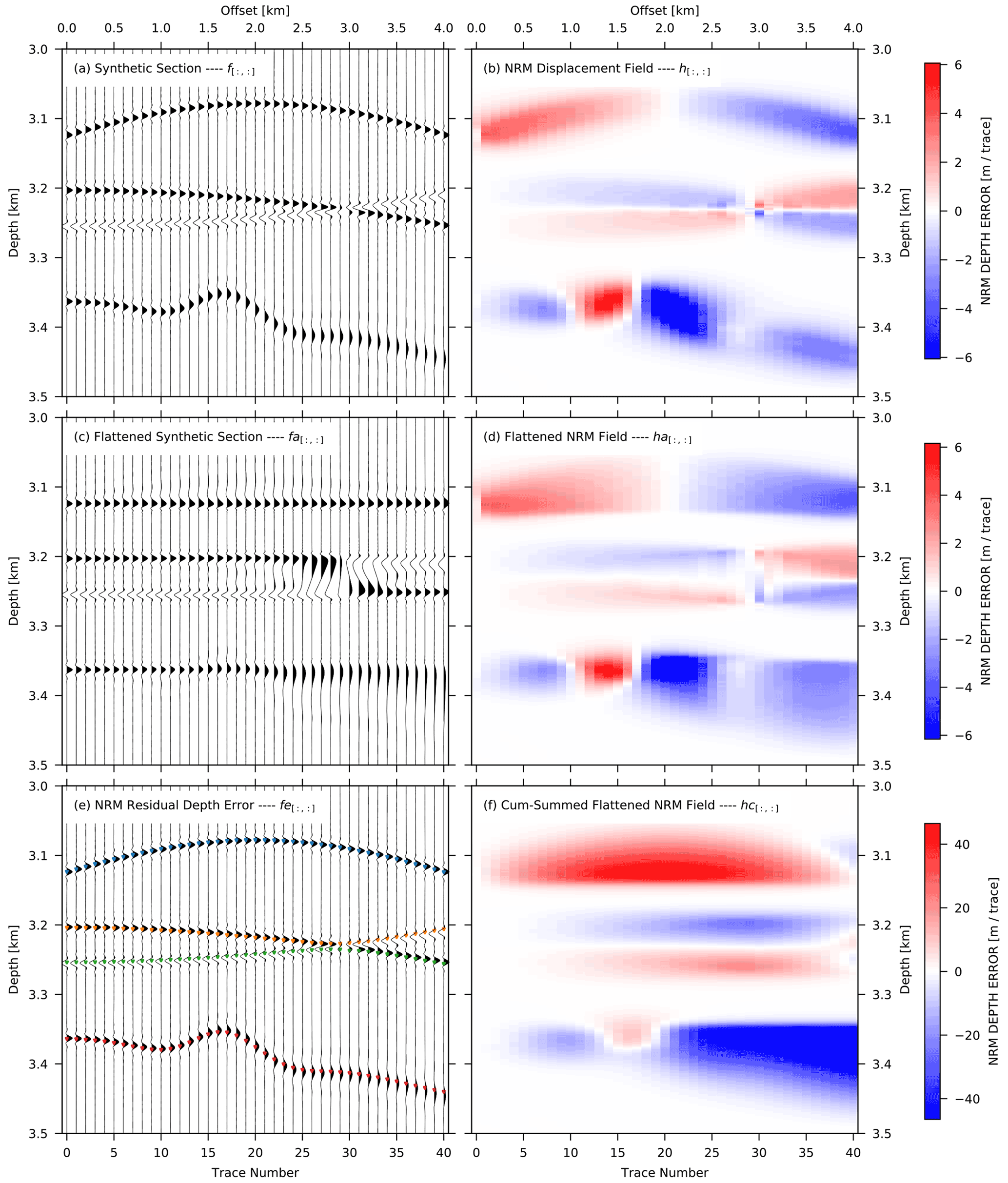
Figure 2(a) Simulated complex geological situations that would be frequently seen in pre-stack depth-migrated (PSDM) common-image-point (CIP) domains. A symmetrical diffraction, two interfering parabolic events with opposite polarity, and parabolic event with a local curvature anomaly, including frequency versus offset signal variations. (b) The relative NRM displacement of gather (a) calculated from trace n to the previous trace (n−1) for n>1. (c) Application of the displacement correction from (b) to the gather of (a). (d) Application of the displacement self-correction of the gather of (b). (e) Residual move-out picks calculated from the recursive cumulative sum of the relative depth errors (f) at predefined nearest-offset depths. (f) Cumulative sum calculated from (d).
Because the NRM displacement field in Fig. 2b is calculated in a relative referenced scheme of a trace to its previous trace, the relative dip displacements correspond to a local dip field. The red colour of positive values in each trace shown in Fig. 2b suggests that a corresponding trace sample in Fig. 2a should be shifted downward to match and align to its previous trace sample by the application of the displacement field values. Blue-coloured negative values require shifting in the opposite (i.e. upward) direction. A zero-displacement value appearing at the apex of the symmetrical diffraction events illustrates the fact that the dipping angle at this location of the event is zero. The NRM field of these three sets of synthetic events follows the general local dip trend well.
2.1.2 Depth-variant alignment from relative displacement correction
Since the NRM field contains the full information of the relative depth-variant shifts of the seismic events, the NRM field can be used to flatten the input seismic section, which has several advantages for the depth error calculation and as quality control of the validity of the displacement field. Intuitively the second trace of Fig. 2a must be depth-variant shifted by the amplitudes of the second trace of the NRM field in Fig. 2b to get aligned to the first trace. To further align the third trace of Fig. 2a, the trace must be depth-variant shifted by the amplitude of the third trace of the NRM field in Fig. 2b and additionally shifted by the previous depth corrections which were applied to the second trace. The following equations are documented in the online repository (https://doi.org/10.5281/zenodo.5998288, Xia et al., 2022) as web-based interactive script files. The depth correction alignment can be written as recursive formula Eq. (5):
where is the original synthetic seismic trace array at the ith trace, represents the NRM displacement field at the ith trace, the index i represents the actual trace number index of the dataset (), and the function Plin represents an irregular linear interpolation function. The function Plin for any corrected sample could be expressed as in Eq. (6):
where the m and n are the closest irregular (non-integer) index to j in the depth corrected index array r[:] by the NRM field for any given seismic trace . Please note that the displacement shifts from seismic amplitudes have much higher precision than the traces' depth sample rate, and the correction of the depth indexes will end up with non-integer numbers in the intermediate index array r[:]. Therefore, an irregular linear interpolation is needed in the calculation to recover the original regular depth index j. The depth index j will be immediately obtained after the linear interpolation.
Based on the above discussion, any intermediate irregular index r[k] in the array r[:] can be simply expressed by , where j represents the original regular depth index of the array , and k represents the index of the NRM-corrected irregular index array r[:], (). Since the element h[i,j] is a number with decimal, the intermediate NRM-corrected index array r[:] does not have to be an integer. Thus, the array r[:] could be simply expressed as follows:
where the represent the NRM displacement field at the ith trace. By applying Eqs. (5)–(7), one could readily get the flattened synthetic seismic section (Fig. 2c). The Python programming with the flattening of the seismic section in Fig. 2c is documented in the online repository.
The NRM flattened events by the recursive depth-variant correction in Fig. 2c provide quality control of displacement calculation for these three special situations. Generally, the squeeze-and-stretch effect of the non-linear displacement correction is inevitable for a multi-trace gather, but as shown here, the displacement shift correction adequately dealt with most of the simulated examples. The first symmetrical diffraction events get optimally flattened, with no significant change of the wavelet shape. The third non-linear undulation with a wavelet variation effect is effectively flattened at the peak amplitude, but strong wavelet stretch is visible. After the NRM displacement correction, the wavelets at mid-offsets (1.5 to 2.5 km) get squeezed and at far offsets (3.5 to 4.0 km) stretched equivalent to normal move-out stretch effects. The crossing region of the two intersecting events is flattened well but suffers from a significant stretch effect, which introduces substantial artificial low-frequency energy between the two events between offset 2.5 and 3.5 km. Due to the constraint that vertical shifts cannot swap neighbouring depth samples, a false event relation occurred beyond 3 km offset, as clearly seen in Fig. 2c by the opposite signal polarity along the two flattened events (between 3.2 and 3.27 km depth). As a result, in a final stacking procedure of this CIP gather, the NRM displacement correction will lead to wavelet stretching, squeezing artefacts, and destructive summation.
An application of the same procedure of Eqs. (5)–(7) to the NRM field instead of the seismic section results in the depth-corrected (flattened) relative NRM displacement field , as shown in Fig. 2d. This flattened NRM field will be used for automatic tracking and picking of the continuous events in the CIP gather.
2.1.3 RMO automatic picking by tracking through NRM displacement field
As the flattened NRM relative displacement field contains the information of relative depth shift from trace to trace along depth slices, the estimation of the depth error is achievable by predefining a start tracking depth at the first trace (nearest offset) and analysing the corresponding depth slice of the flattened NRM field in Fig. 2d. Given a pre-defined starting pick z0 at the nearest offset, the change of the residual reflector depth , which is needed for the reflection tomography, can be extracted along the flattened NRM displacement field by calculating a cumulative summation along the depth slide at depth z0:
where the array Δz[:] represents the depth error relative to reflector depth z0, array represents the depth-corrected cumulative-summed NRM displacement field, and the index i represents the trace number. For any trace in Fig. 2d the cumulative summed NRM field in Fig. 2f can be calculated by
The array represent the ith flattened NRM trace. With the knowledge of the residual reflector depth , one could readily get the RMO of any reflector in a seismic gather:
where array represents the absolute depth of an RMO sequence over the gather for a series of continuous reflectors. By applying Eqs. (8)–(10), and using the simple synthetic seismic (Fig. 2a), the four series of RMO picks illustrated in Fig. 2e represent the auto-tracked RMO depth of the events. The Python programming of Eqs. (8)–(10), the calculation of the RMO of a series of continuous reflectors (Fig. 2e), and the absolute NRM field calculation (Fig. 2f) are documented in the online repository (https://doi.org/10.5281/zenodo.5998288, Xia et al., 2022) as web-based interactive script files.
As a result, all RMO depth error picks follow the amplitude peaks of the seismic events except for the “X”-shaped interfering reflectors. The NRM displacements are misled by the crossing point and switch to an event that should not be followed. This kind of “V”-shaped depth error information will undermine the reliability of the tomographic result because the depth error branch is a combination of two different events. To avoid this mismatch a quality factor is introduced and assigned to each individual pick along the depth error branch. A sliding trace summation window along a depth slice or comparison of a near-offset stack to the individual events can be used. In this example, a sliding trace summation would detect a rapid decrease in quality due to the polarity change resulting in a destructive summation. Picks with lower quality as a predefined threshold can be deleted. In this special case, the two depth error branches of the intersecting events will be split into four individual depth error branches which the reflection tomography will handle correctly as four independent reflection events. If these crossing events happen as a result of interfering noise like surface-related or interbed multiples, the unwanted events should be attenuated prior to NRM by a dip filter in the CIP gather (Fig. 1).
To verify the accuracy of the NRM method we compared the picking results of the NRM method to a plane-wave destruction filter PWD method (Fig. 3). The PWD method is splitting the data into spatially and temporal windows and assumes that the slopes are stationary within each window (Fomel, 2002; Xue et al., 2019). In contrast, the NRM method is iteratively minimizing the amplitude difference (Eqs. 1–4) between an adjusted gather and a reference gather for all events simultaneously. For both methods, the estimated depth error picks in Fig. 3a are near the maximum amplitude peak of the events. On the far offset traces with reduced amplitudes the NRM shows less accuracy (Fig. 3b). Due to the strategy by the NRM method to minimize the band-limited amplitude difference, the strongest near-offset amplitude events will dominate this inversion result. This strategy is useful by comparing two seismic cubes with a special focus on depth or spatial shifts to reduce distortions from low-amplitude events. To avoid small-amplitude events in a CIP gather being underdetermined in their dip estimation an additional gain balancing is recommended before an NRM application.
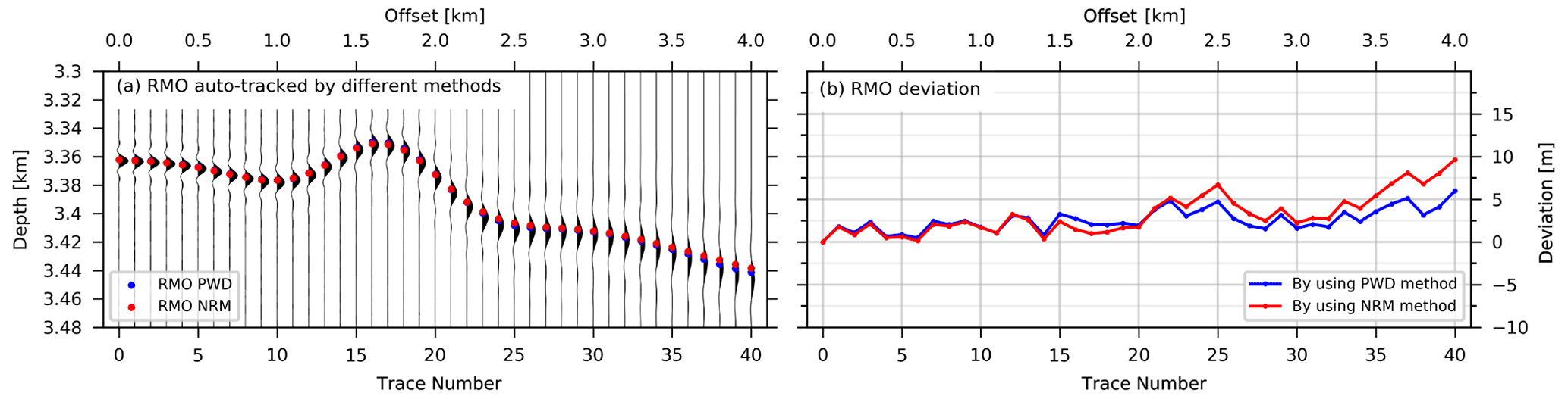
Figure 3(a) Comparison of residual depth error picks between the NRM and PWD method. (b) Depth difference between the depth errors of the NRM and PWD method.
2.1.4 Effective RMO selection based on semblance analysis
Giving predefined starting depths for the RMO tracking is applicable in a simple synthetic test which contains only few continuous reflectors. However, it is unrealistic to define each reflector's starting depth in real data or complex synthetic examples, which could have several tens of effective reflectors in one migrated CIP gather (Fig. 4a). An efficient approach to determine the reflectors' start-tracking depth is by analysing the flattened CIP gather (Fig. 4c) by a semblance-weighted grid-based scheme.
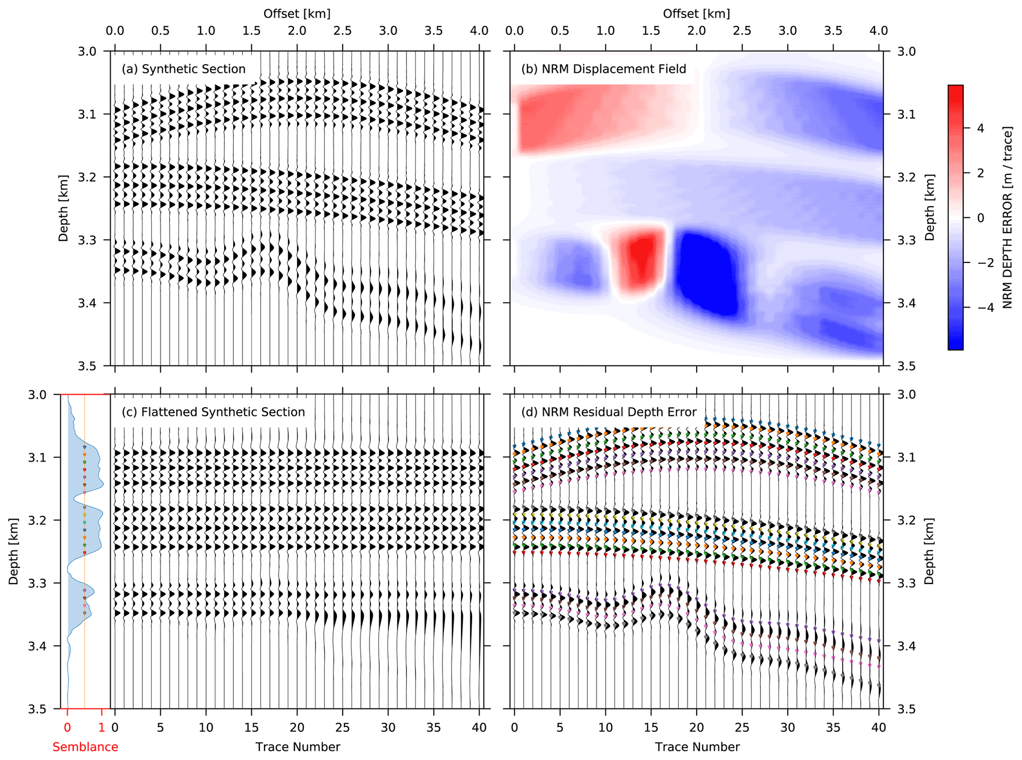
Figure 4(a) Simulated geological situations with multiple sets of reflectors. (b) The NRM displacement of gather (a) calculated from trace n to the previous trace (n−1) for n>1. (c) Application of the “relative-displacement correction” scheme from (b) to the gather of (a). (d) Residual move-out picks automatically calculated by the semblance-weighted grid-based approach of the relative depth errors of (b).
A semblance s[j] value, which is a quantitative measure of the similarity of a number of traces (Yilmaz, 2001) in the seismic section, is described as follows:
where n is the maximum number of traces, F[i,j] represents the seismic section, the index i represents the trace number, and the index j represents the sample depth.
By conducting semblance calculation on the NRM-flattened seismic section (Fig. 4c), the flattened section could not only provide NRM field's quality control but also sheds light on selecting effective reflectors and determining the starting depth for RMOs' auto-tracking. By calculating the semblance value for each depth slice along the flattened seismic section, one can reject unwanted picks, by setting up a threshold of semblance limitation (e.g. 0.5). In the synthetic example with several reflectors (Fig. 4a), RMO picks are digitized in zones of good reflector continuity (semblance >0.5 and minimum pick depth increment of 12 m; see coloured dots in the left panel of Fig. 4c) and rejected in non-reflection or weak zones (semblance <0.5) (Fig. 4d). The math applications of this auto-picking and semblance threshold selection schemes are documented in the online repository (https://doi.org/10.5281/zenodo.5998288, Xia et al., 2022).
Because the plane-wave destruction filter (PWD) is widely used to estimate the move-out dip slopes on seismic sections or gathers (Fomel, 2002; Sripanich et al., 2020), we applied the outlined processing sequence of displacement corrections based on a PWD filter in the online repository as an alternative method to the NRM method.
2.2 Methodology of the ray-based grid tomography with CIP depth errors
The basic concept of iterative ray-based grid tomography is to find subsurface velocity perturbations that minimize the residual move-out depth error picks of the initial migrated CIP gathers (Woodward et al., 2008). Conditions that must be fulfilled are preserved arrival times. The calculated arrival time t of ray path for a given depth error pick Δz through the initial velocity model must be preserved in the updated velocity model. That requires that a change of the residual reflector depth Δz must be compensated by small changes in the velocity model Δαi where the index i corresponds to a grid node in a gridded model. For an acoustic reflection it follows the residual migration equation of Stork (1992):
Here Δt is the preserved arrival time, Δz is a change in reflector depth, Θ is half the opening angle between source and detector rays at the reflector, Φ is reflector dip, and α the velocity at the reflector depth of the actual model. Δαi is a change in the velocity, and is a change in travel time corresponding to a change of velocity α at grid node i. As is calculated independently of the ray parameters Θ and Φ, the ray path bending is assumed not to change during a velocity update. From this follows that only small velocity perturbation should be estimated for each iteration step.
The CIP tomography must find the velocity change Δαi that is needed to flatten migrated reflectors and eliminate the picked reflector depth error for each offset h to a new depth based on Eq. (12):
Due to the unknown residual migrated depth , the CIP tomography minimizes the difference (), where h=0 is the nearest offset of a picked depth error branch, not necessarily zero offset, and h a non-nearest offset. This yields to Eq. (14):
We have a set of linear equations for each pick zh at offset h along a depth error branch relative to the nearest pick z0 for offset 0 along the depth error branch and that for many depth error branches along the whole profile. The tomography equation in matrix notation is written in Eq. (15),
where P weights individual depth error areas, L is the matrix of the ray path term calculated by the residual migration term in brackets of Eq. (14); S is a scale length smoother with the predefined wavelength in lateral and vertical direction; SΔα together is the velocity update vector, W is a damping factor allowing the update magnitude of the model to be adjusted, and Δz is our accumulating picked depth errors between non-near and near-offset picks. The aim of the reflection tomography is now to solve the equation to find a Δα that will explain the residual depth errors Δz. The residual depth errors are usually picked manually or automatically tracked by linear or hyperbolic assumptions. While the latter approach is convenient, it needs additional parameters, especially for non-hyperbolic or weak events. Typically, coherence measurements are used and additional outliners must be detected and removed. Despite this, a vertical and spatial smoothness between depth error branches is not guaranteed. Using the application of the NRM-based picking the smoothness of the depth errors Δz in space and depth will be guaranteed and stabilize the linear equations and the inversion result. Additional regularization and weighting schemes also need to be applied to find a velocity change Δα that will minimize Eq. (15). Details can be further seen in Woodward et al. (2008).
The choice of the parameters of weight P, smoothing scale length S, and damping factor W are strongly data dependent. Tomographic inversion works by iterative velocity updating to minimize the observed residual velocity error (Eq. 15). In the CIP gathers, the depth errors are distributed over the entire offset range and yield the estimation of the interval velocity changes along their ray paths between the source and receiver (Jones, 2010). Due to the linearized approximation in Eq. (14), by ignoring the ray path bending during the estimation of the velocity update, several iterations with only small velocity updates (e.g. ∼10 %) are recommended. Additionally, a large volume with a high spatial density of the residual depth errors needs to be picked in order to stabilize the linear equations by the redundancy of information (Jones, 2003). Once there is a conflict occurring between some of the equations in one grid cell, the minority picks (which could be good or bad) will be rejected by the tomography algorithm in order to get a stable and self-consistent result. Unrealistic picks have an unfavourable effect on the tomographic results when they become the majority. Besides the pick density and depth error accuracy Δz, the smoothing scale length S is the most important parameter for the grid tomography.
If the initial velocity is not well determined, e.g. smoothed depth-converted stacking velocities or depth-converted pre-stack time migration velocities, a long-wavelength to short-wavelength velocity update is a preferred strategy by reducing the smoothing scale length S in Eq. (15). The first iteration is applied with a spatial smoothing length covering at least twice the CIP ray path coverage aperture to update the long-wavelength velocity structure only. In the following iterations, the scale length is successively reduced for each iteration to receive increasing velocity details as shown in Woodward et al. (2008).
If an initial background velocity is well determined, e.g. depth-focusing analysis from pre-stack depth-migrated data, each iteration can be applied immediately with multiple scale lengths, starting from the longest to shortest scale length for each velocity update. Independent of the grid-based reflection tomographic inversion strategy it is common to stop the iterations if an iteration does not contribute any more to the flatness of the CIP residual move-out. Qualitative control will give a comparison of the reflectors' horizontal alignment in the CIP gather with respect to a previous iteration or initial iteration. A more quantitative measure to stop an inversion is to define a lower limit of percentage velocity change which must be achieved (e.g. 3 %).
In contrast to the grid-based tomography, where vertical and horizontal velocity gradients are determined during the inversion, the layer-based tomography updates the lateral velocity variation between two user-defined horizons with a predefined vertical velocity gradient. A comparison of layer-based and grid-based tomography results can be found in Riedel et al. (2019) and Sugrue et al. (2004). Model areas in which a priori velocities are known (e.g. the water column above the seafloor) and hybrid models are used to avoid tomographic velocity updates propagating into selected areas. Furthermore, first-order velocity contrasts, resulting in ray-path bending are problematic as they cannot be inverted by finite grid size. Here hybrid models delivered the best results as shown by Jones et al. (2007) and Fruehn et al. (2008). For most of the studies it is common that the grid-based tomography was applied to moderate layered structures in combination with the hyperbolic curvature scanning technique from Hardy (2003) to estimate the depth error in the CIP domain. An application result of a grid-based tomography combined with the NRM technique in a moderate layered structure is shown in Crutchley et al. (2020).
An application of the NRM common image point depth error estimation in combination with an iterative grid-based tomography approach will be presented here in detail for three different structural settings along a profile crossing the Java trench. The complexity of the data examples increases from moderate horizontal layering, to dipping layered reflections, up to small disrupted dipping reflector elements.
In contrast to the processing by Lüschen et al. (2011), where the velocity model was built iteratively from interpreted depth-focusing analysis in a top-down approach, we used a wide-angle tomography model as initial velocity in combination with a data-driven grid-based reflection tomography. The use of wide-angle and refracted velocities may be influenced by anisotropy but gives the most confident velocity in the deeper subsurface due to the limited streamer length.
3.1 Study area and MCS data pre-processing
The multi-channel 2-D reflection seismic profile BGR06-313 that we use in three field examples was acquired by a 3000 m long, 240-channel digital streamer with a group distance of 12.5 m at a towing depth of 6 m. A two-string G-Gun array of 3080 in.3 (50.8 L) volume with a nominal shot point distance of 50 m was used as a source across the southern Java trench in the south-eastern part of the Sunda subduction zone (Lüschen et al., 2011) as part of the SINDBAD project during RV SONNE Cruise SO190 (Fig. 5).
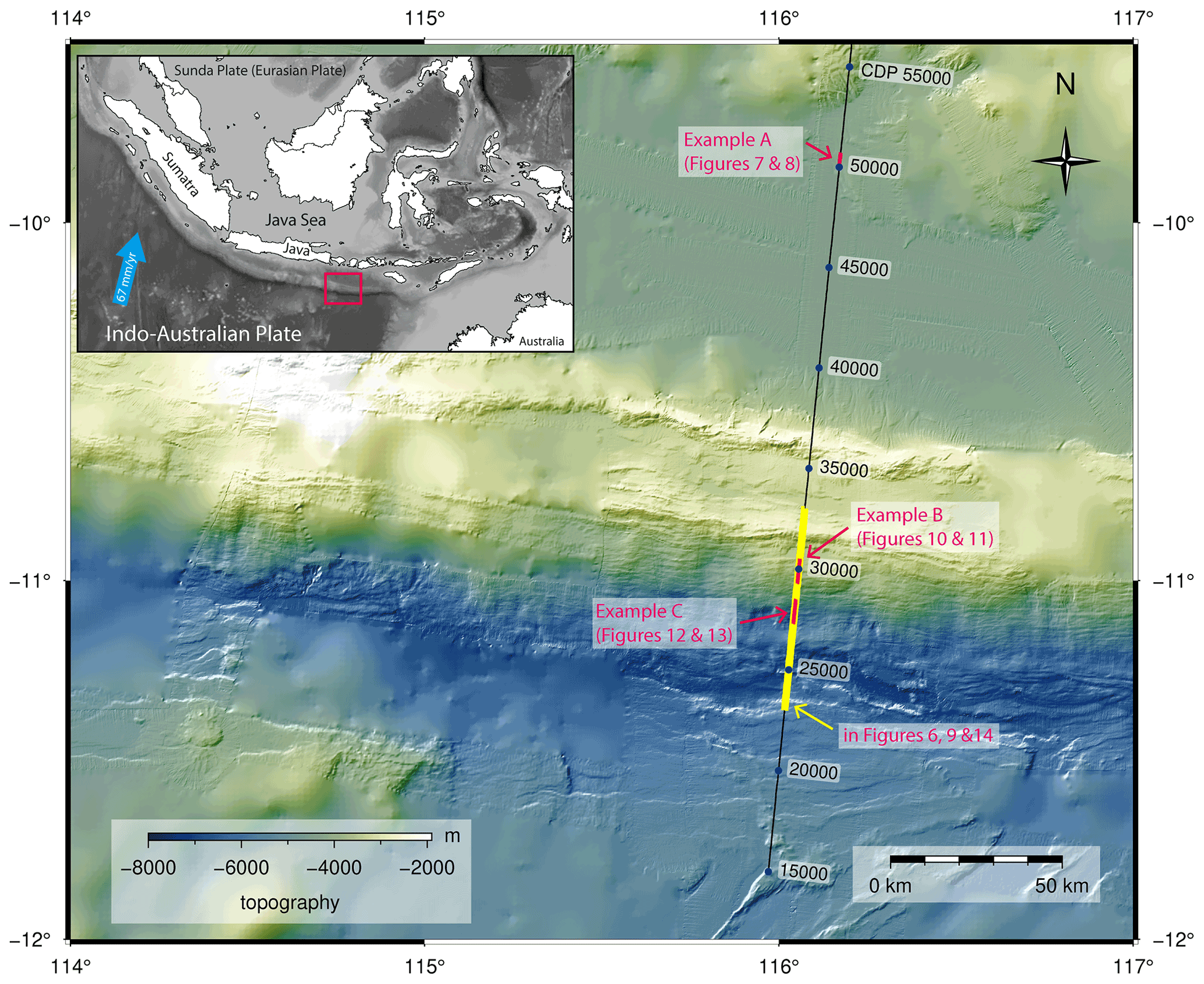
Figure 5Map of the study area offshore southern Java, created by the authors using the open-source software Generic Mapping Tools (GMT). Local multi-beam bathymetry data were acquired during the SO190 cruise and overlain on the global GEBCO_2020 grid (GEBCO Bathymetric Compilation Group, 2020). The location of the multi-channel and collocated wide-angle seismic profile is shown by a black line. Three examples at locations A, B, and C (marked in red) of the NRM-based velocity update for the depth tomography and pre-stack depth migration result are discussed in detail. Example A is located at shallow depth with simple complexity, whereas examples B and C are crossing the subduction trench and accretionary wedge (yellow line) and show highly complex structures where standard velocity analyses mostly fail because of discontinuous highly dipping structures.
The seafloor depth ranges from 1.5 km near the shore on the northern part of the line to 6.5 km in the deep-sea trench. Details of our seismic processing sequence are provided in Table 1. In preparation for the Kirchhoff PSDM, the multiple reflections have been attenuated using a free surface multiple prediction (Verschuur et al., 1992) followed by a frequency-split 2-D adaptive least-square subtraction (Robinson and Treitel, 2000; Guitton and Verschuur, 2004), and a Radon transform dip filter (Hampson, 1986).

3.2 Initial velocity building from wide-angle tomography
The initial velocity model for the reflection depth tomography was merged from an OBS velocity tomographic inversion of a collocated 2-D refraction seismic line covered by 46 OBSs with a spacing of 6 km (Planert et al., 2010) and a velocity model estimated from the near-seafloor structure at coarsely sampled CMP locations by interactive semblance velocity analysis. This near-subseafloor velocity adjustment was needed because the MCS reflection and OBS acquisitions were split into two cruise legs and both profiles did not completely coincide as seen by the mismatch of the seafloor depth at the lower slope and the trench axis (Fig. 6a). Due to a gap of three OBS positions in the trench axis the velocity structure was not well determined near the trench axis with lower-slope sediment velocities of more than 3800 m s−1 between CDP 25 000–26 500 at a depth of 7000 m (Fig. 6). In the first step, the MCS velocity analysis was based on pre-processed CMP gathers and interactively picked semblance with an increment of 500 CMP locations. Based on this smoothed stacking velocity a pre-stack time migration was subsequently applied and a second interactive semblance velocity analysis on the migrated CIP with the same increment delivered a smoothed and depth converted velocity model for the upper 2 km below the seafloor. To finalize the initial tomography model building, the adjusted velocity at shallow depth was merged with the wide-angle velocity model and used for the following NRM tomography (Fig. 6b).

Figure 6(a) The original OBS velocity model with the line drawing based on the final PSDM image. (b) The initial velocity model for the reflection tomography merged from the multi-channel seismic velocity analysis above the white transparent band and the wide-angle velocity model (below the white transparent band). The line drawing is based on the final PSDM image.
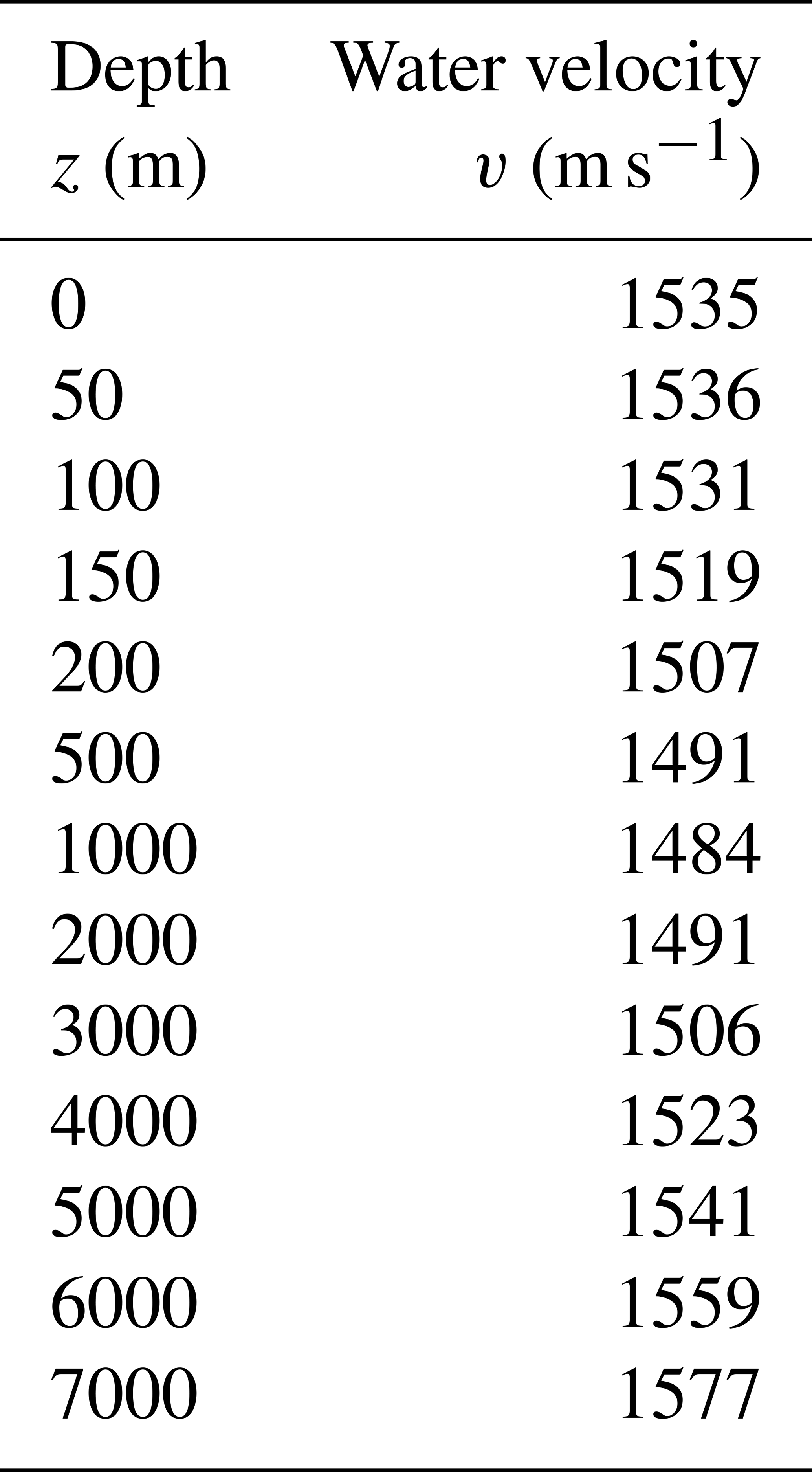
As an additional constraint for the tomography, a hybrid model with the seafloor as a fixed boundary was chosen to avoid velocity changes propagating into the water column, resulting in depth changes of the seafloor. This was especially needed at the trench axis where side reflections and cross-dipping structures due to the rough seafloor topography were observed (Fig. 5). A regional depth-variant water velocity (Table 2) was extracted from the Climatological Atlas of the World Ocean multibeam (MB) system (Levitus, 1983) and used for the entire profile.
Table 2Regional depth-variant water velocity extracted from the Climatological Atlas of the World Ocean MB system (Levitus, 1983).
It should be noted that the wide-angle velocity could not be updated at a depth greater than 4 km below the seafloor during the initial velocity building and the subsequent reflection tomographic inversion since the limited streamer length (3 km) does not provide enough residual move-out sensitivity.
3.3 Reflection tomography attribute data
For the automatic residual NRM picking (see Fig. 4c, d from the synthetic example) an initial depth slice increment of 50 m for the residual depth error pick tracking through the NRM displacement field was depth adjusted based on minimum threshold semblance values by scanning along offsets of the CIP gather.
One attribute presented for the tomography is the reflector dip field Φ (Eq. 14) of the migrated section, which determine the ray coverage propagation direction (see Fig. 7e as an example). A second attribute is the spatial variant weight function W (Eq. 15) calculated from the spatial coherency (Fomel, 2002; Neidell and Taner, 1971) of the depth-migrated structure to weight the picks of the depth error branches (see Fig. 7f as an example).
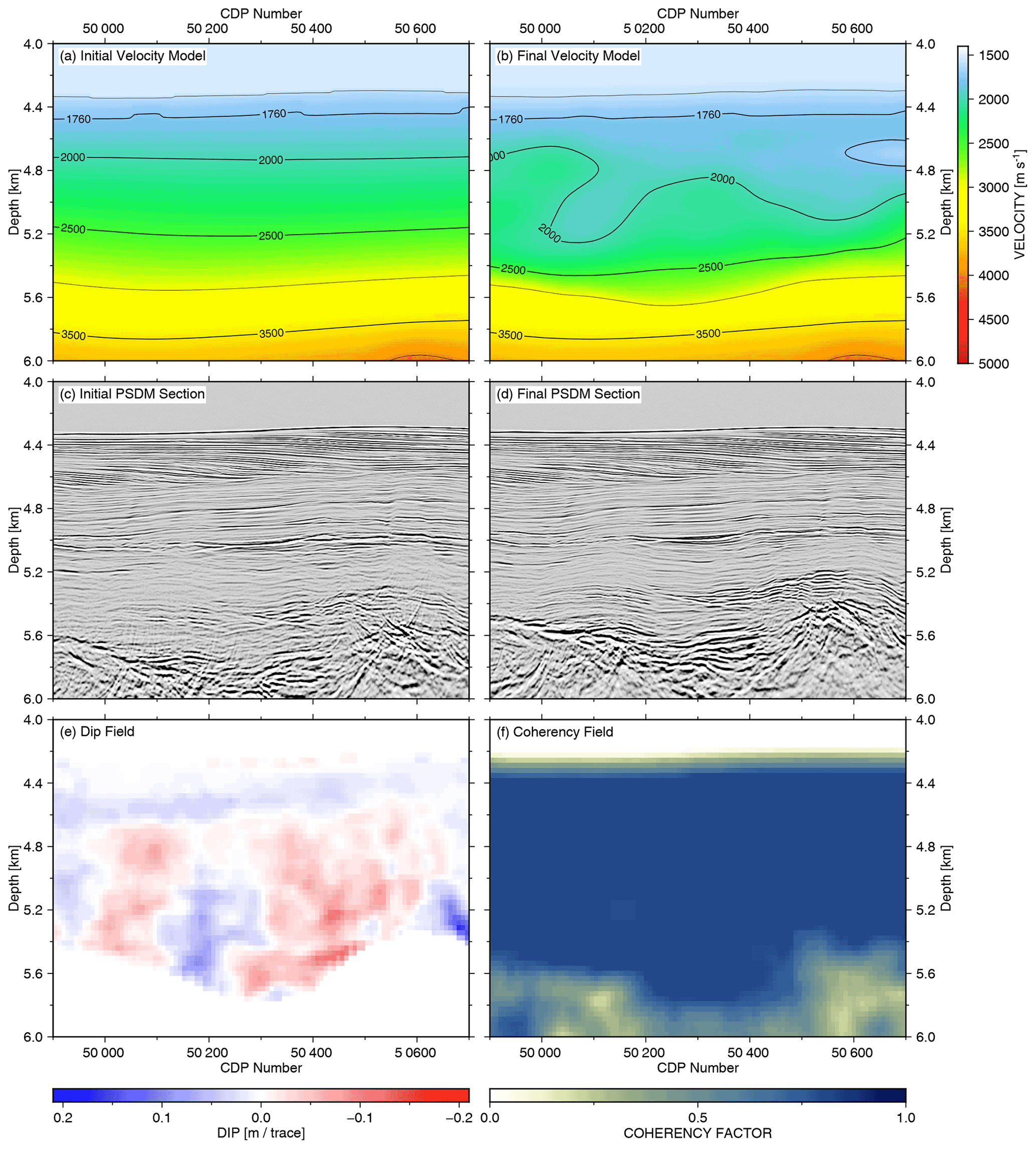
Figure 7Depth tomography example A from Fig. 5, with CDP ranging from 46 700 to 50 800. (a) Initial velocity model merged from velocity analysis and wide-angle refraction tomography. (b) Final velocity model after five iterations of NRM-based depth tomography and PSDM. (c) PSDM result based on the initial velocity model. (d) PSDM result based on the final velocity model. (e) Reflector dip field calculated from the final PSDM result. (f) Reflector coherency field calculated from the final PSDM result. Note that “migration smile” artefacts at a depth of 5.6 km in (c) are significantly reduced in the final PSDM result (d).
3.4 Data examples
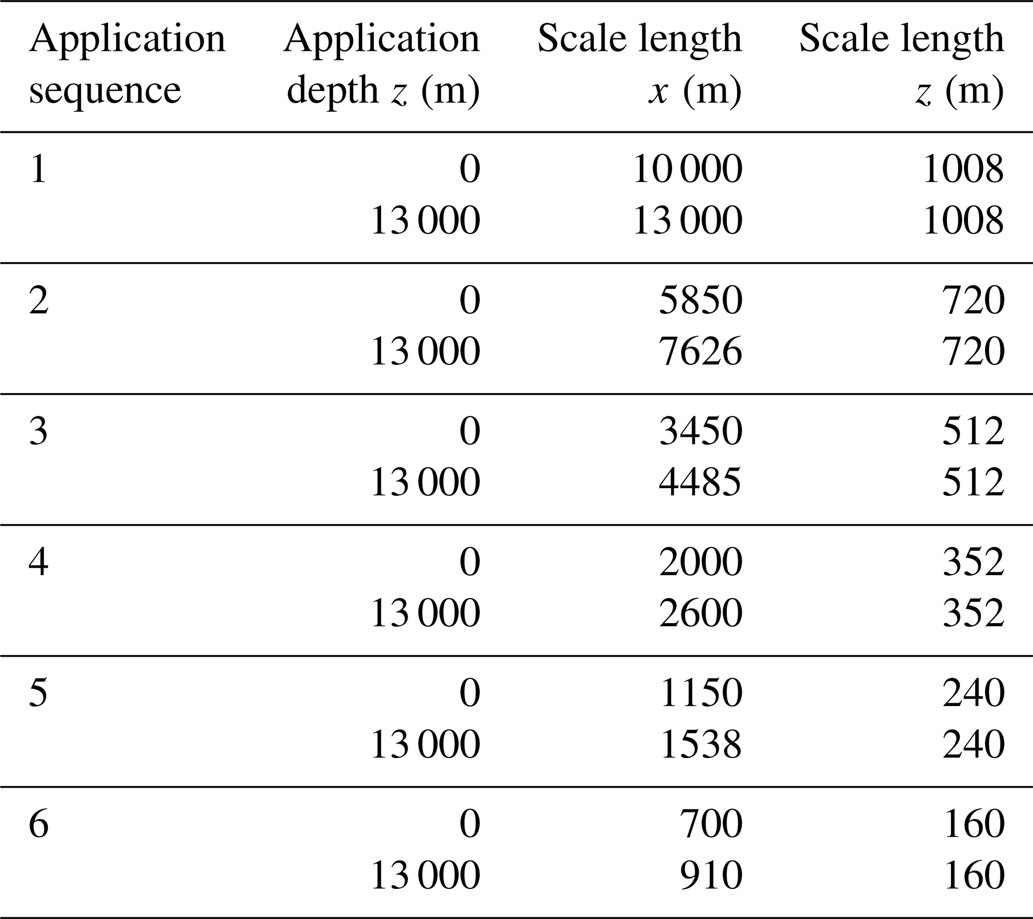
Each iteration loop in the tomographic processing flow (Fig. 1) included approx. 11 000 depth error branches, each branch with 30 picks, and six sequentially applied scale-length smoothings S (Eq. 15). Starting from the longest down to the shortest application sequence, each smoothing was applied over the complete depth range (Table 3). In total five iterations of velocity updates were applied, where for the following presentation only the initial and the final results are shown for the purpose of comparison.
Table 3Successive smoothing scale length reduction applied for each iteration of the depth tomography.
In the data examples, we show three different structural settings with results of the velocity model, the corresponding PSDM sections, and the NRM displacement field, as well as the spatial coherence field together with the reflector dip field of the final migrated section. To document the change in the CIP-gather domain in detail, we additionally compare selected subareas of initial and final CIP gathers, the calculated NRM displacement fields, and the residual depth error picks, as well as on overlay display with the CIP gather and the depth error picks.
3.5 Sediment basin NRM tomography
The first field data example, “Example A”, at the northern end of the profile (Fig. 7), is a shallow sediment basin with layered interfaces and continuous reflectivity and represents an optimal site to obtain a reliable velocity model in a 2-D multi-channel seismic survey. A CIP-gather increment of 32 (200 m) was analysed along the profile with the NRM method. In total, five iterations of tomography loops (Fig. 1) were applied to this data example. An enlarged view of the initial velocity model ranging from CDP 46 700 to 50 800 is displayed in Fig. 7a. The resulting initial Kirchhoff pre-stack depth migration (Fig. 7c) retrieves a coherent image of the shallow sedimentary portion, while the energy in the deeper part close to the basement is not very well collapsed, resulting in a series of over-migrated events. The displayed reflector dip field (Fig. 7e) and coherency field (Fig. 7f) are extracted from the final migration section.
The reflector dip is used for the ray propagation direction during the tomography, and the coherency field is used as an additional weighting of RMO depth error picks in spatially coherent subsurface areas. The two attribute fields were recalculated for each iteration of the tomography loops (Fig. 1). After five iterations of the NRM-based depth tomography and Kirchhoff PSDM, the reflection energy is much better collapsed and shows more focussed and continuous signals, especially in the deeper part between 5.2–5.6 km (Fig. 7d). Furthermore, the final velocity model (Fig. 7b) displays lateral velocity variations that mimic the form of the base of the sediment basin. This is well demonstrated by the 3000 m s−1 velocity contour that mimics the shape of the boundary between the highly reflective basement (below) and the less reflective but more laterally continuous reflections of the sedimentary sequence (above).
Moving into the pre-stack CIP domain, a series of CIP gathers ranging from CDP 49 000 to 50 600 (same profile range as in Fig. 7) are selected and displayed in Fig. 8a with an increment of 32 (200 m). A dip filter is applied to the gathers to eliminate the extreme dipping events and migration noise. The NRM field in Fig. 8c shows the initial relative displacement values for each data sample. The information below the basement is muted by a digitized basement horizon. The distinct block of blue colour within the red rectangle in Fig. 8c, at a depth of 5.0 to 5.8 km, illustrates a general velocity overestimation in the overlying sediment. The RMO depth error picks calculated from the NRM displacement field, as a data-driven automatic picking method without any assumption of its curvature, are the main input information for the tomography (Fig. 8e). Figure 8b, d, and f show the final flattened CIP gather, NRM displacement field, and RMO depth error picks, respectively.
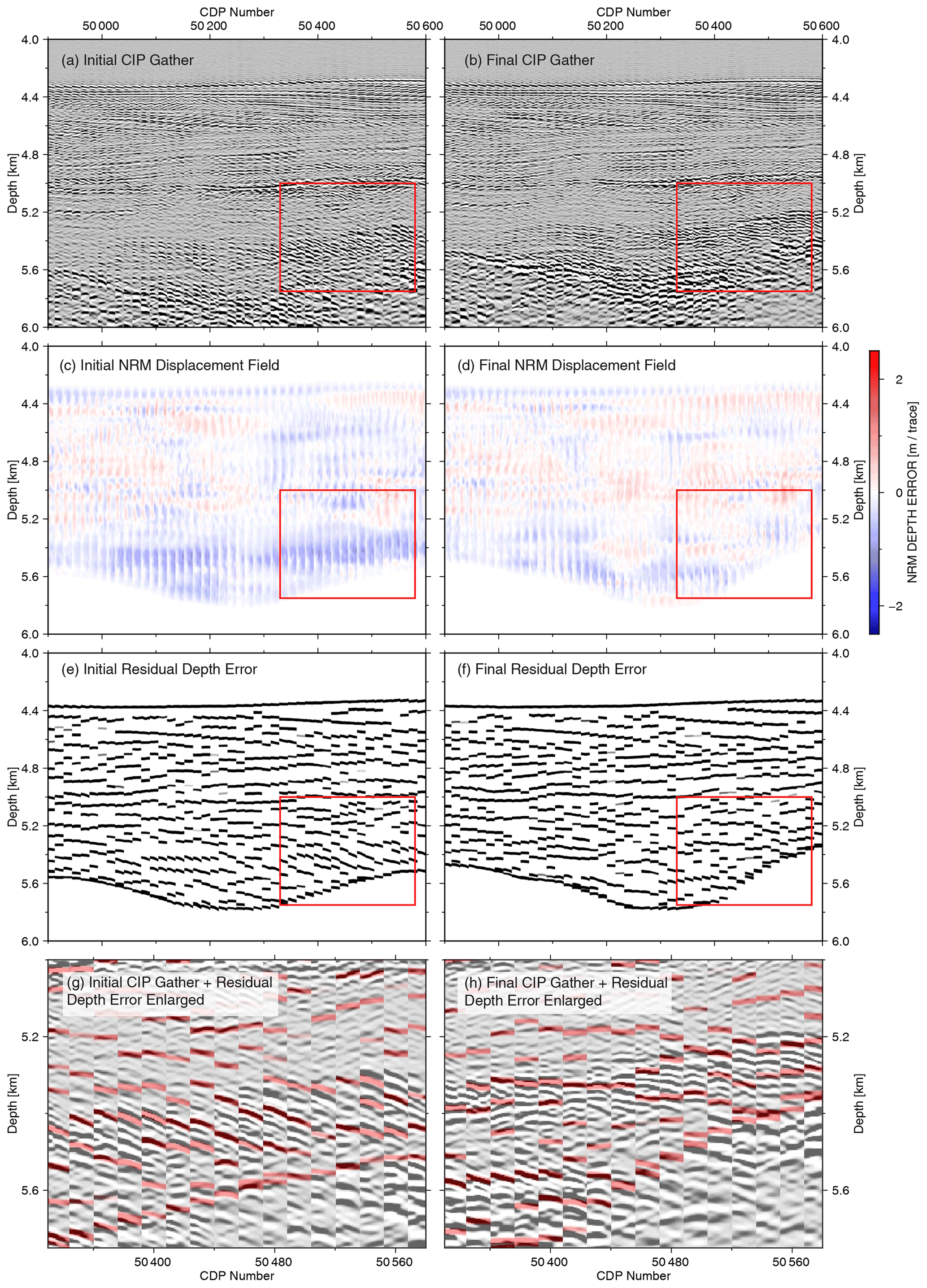
Figure 8NRM velocity updating of Fig. 7 in CIP domain. (a) CIP gathers based on the initial velocity model. (b) CIP gathers based on the final velocity model. (c) Initial NRM depth shifts in the CIP domain. (d) Final NRM depth shift in CIP domain. (e) RMO picks calculated from the initial NRM displacement field. (f) RMO picks calculated from the final NRM depth displacement field. Note that the overall shift error within the distinct area of velocity overestimation in the red rectangle in (c) has been substantially reduced after the tomography (d). CIP gathers (e) and (f) of the red rectangle from (c) and (d) respectively overlaid by RMO picks. Strong dipping events in the initial CIP gather (g) have been flattened after the final iteration (h).
Compared to the initial data, the updated events in the CIP gather become optimally flattened. The depth of the basement shifts upwards by 0.2 km due to the velocity reduction of the final model. In the final NRM field (Fig. 8d), the velocity overestimation error in the region of the red rectangle is substantially reduced. However, some residual move-out undulations from the initial to the final stage remain, as seen in detail in Fig. 8g and h from the CIP gathers overlain with the RMO depth error curves. Ideally, the final NRM displacement field in Fig. 8d should have no NRM depth shift anymore, and all depth error picks should align horizontally. This cannot always be achieved, as the tomography finds only the solution that minimizes the depth error with respect to the smallest scale lengths (Table 3).
3.6 Accretionary wedge NRM tomography
In the following, the PSDM profile (location marked by the yellow line in Fig. 5) with the final velocity model overlain in Fig. 9 will be further analysed.
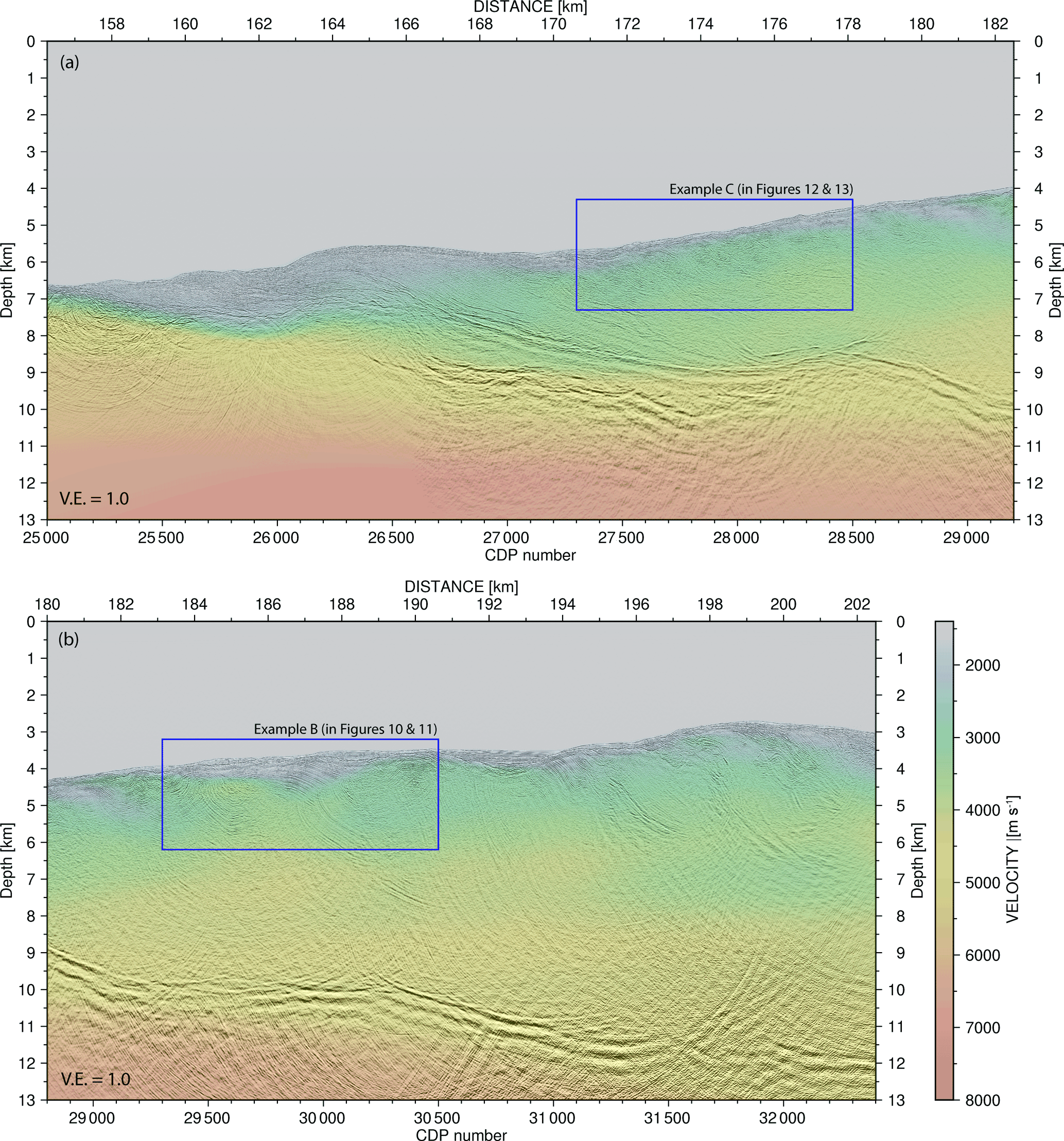
Figure 9Depth migration stack section of five iterations depth tomography with final velocity model overlain. The location of the profile is illustrated in Fig. 5 as a yellow line. Rectangular boxes are discussed in the section on field data examples from the accretionary wedge. (a) Data example C. (b) Data example B.
Two data examples (Fig. 5, examples B and C, marked in red) in the blue rectangles within the accretionary wedge in Fig. 9 show distinct levels of complexity. The selected upper-slope area is characterized by strongly folded continuous reflector sequences, whereas the lower-slope area contains only short reflector segments with varying dips. The lack of coherent reflective signals in this highly deformed accretionary prism leads to a severe difficulty in accurately evaluating the residual move-out in the CIP gathers, especially if a constant spatial analysis increment (e.g. 500 CDP = 3125 m) is greater than or equal to the lateral dimensions of velocity structures to be resolved (e.g. the piggy-back basin CDP 30 500–31 000, 3 to 4 km depth in Fig. 9b). As a consequence of the spatially complex reflectivity pattern, the automated CIP analyses were reduced to an increment of 16 (100 m) to achieve more redundancy of depth error estimations during five iterations of the tomography.
3.6.1 Upper-slope NRM tomography
Our second field data example focuses on a sequence of thick sediment tilted by compressive deformation in the region marked by the blue rectangle example B in Fig. 9b. Figure 10 provides a detailed image of the PSDM section and velocity model from the initial and final stages. The final velocity (Fig. 10b) is significantly reduced compared to the initial velocity model (Fig. 10a) in the shallow part and significantly increased compared to the initial model at depths of 5.2–6.2 km. The reflector sequences of the anticline structure between CDP 29 300 and 29 500, from 4.0–4.4 km depth, are more continuous in the final image (Fig. 10d) than in the initial image (Fig. 10c), especially at the top of the anticline. The dip of the folded reflector sequence between CDP 29 800 and 30 100, above 4.8 km, is more continuous in the final image (Fig. 10d), since the residual depth error is better flattened (Fig. 11g and h), and the reflector dip in the PSDM section increases steadily with increasing distance from the apex of the fold (Fig. 10d). By contrast, the initial image in this same region (Fig. 10c) shows an abrupt change in the dip near the apex of the fold.
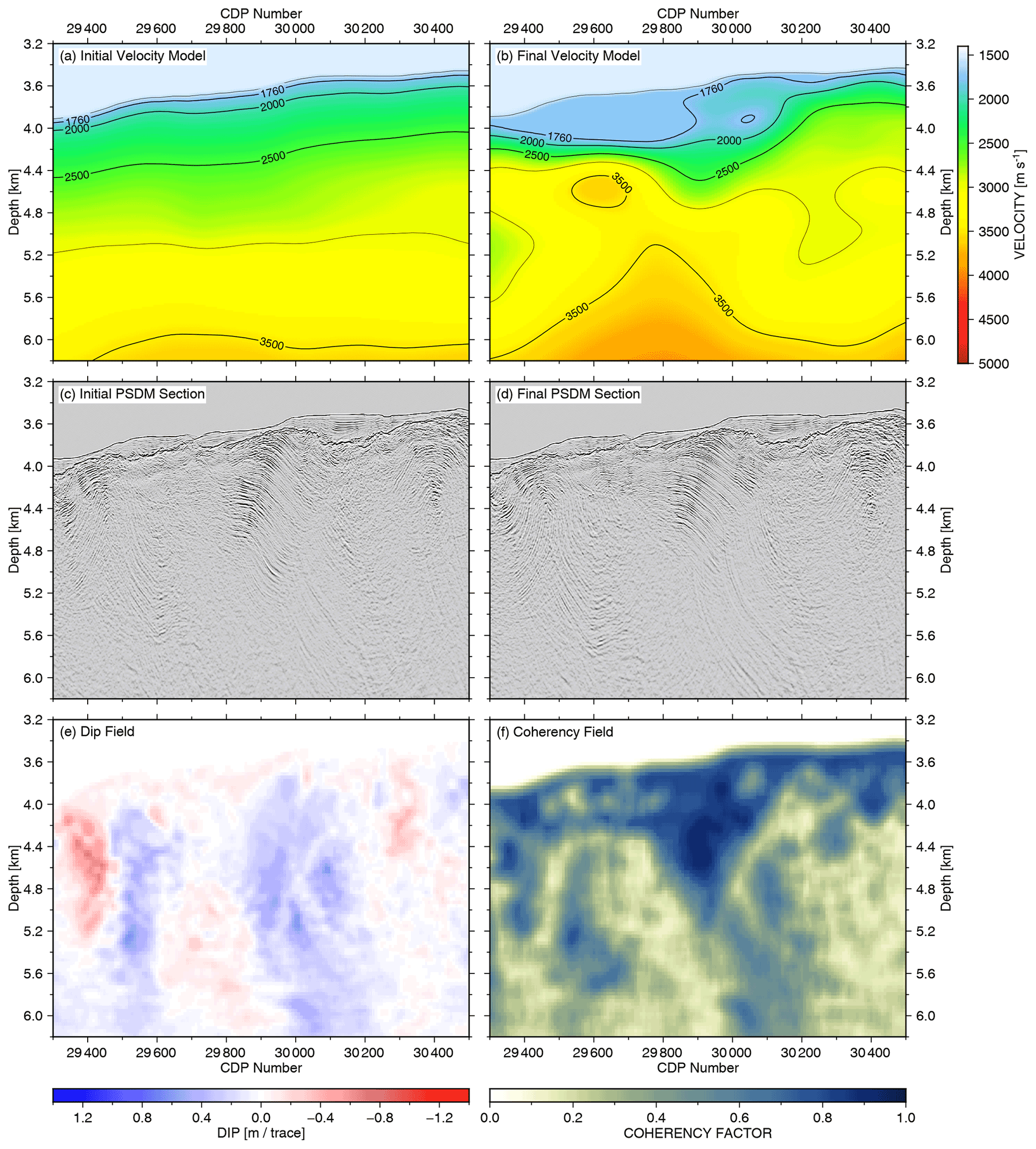
Figure 10Depth tomography example B in Figs. 5 and 9b, with CDP ranging from 29 300 to 30 500. (a) Initial velocity model merged from velocity analysis and wide-angle refraction tomography. (b) Final velocity model after five iterations of NRM-based depth tomography and PSDM. (c) PSDM result based on the initial velocity model. (d) PSDM result based on the final velocity model. (e) Reflector dip field calculated from the final PSDM result. (f) Reflector coherency field calculated from the final PSDM result. Notice the continuity and reflector dip change of the folded sediment layers at a depth of 4.0–4.8 km in (c) and (d) based on the change of the initial velocity and final velocity (a) and (b), respectively.
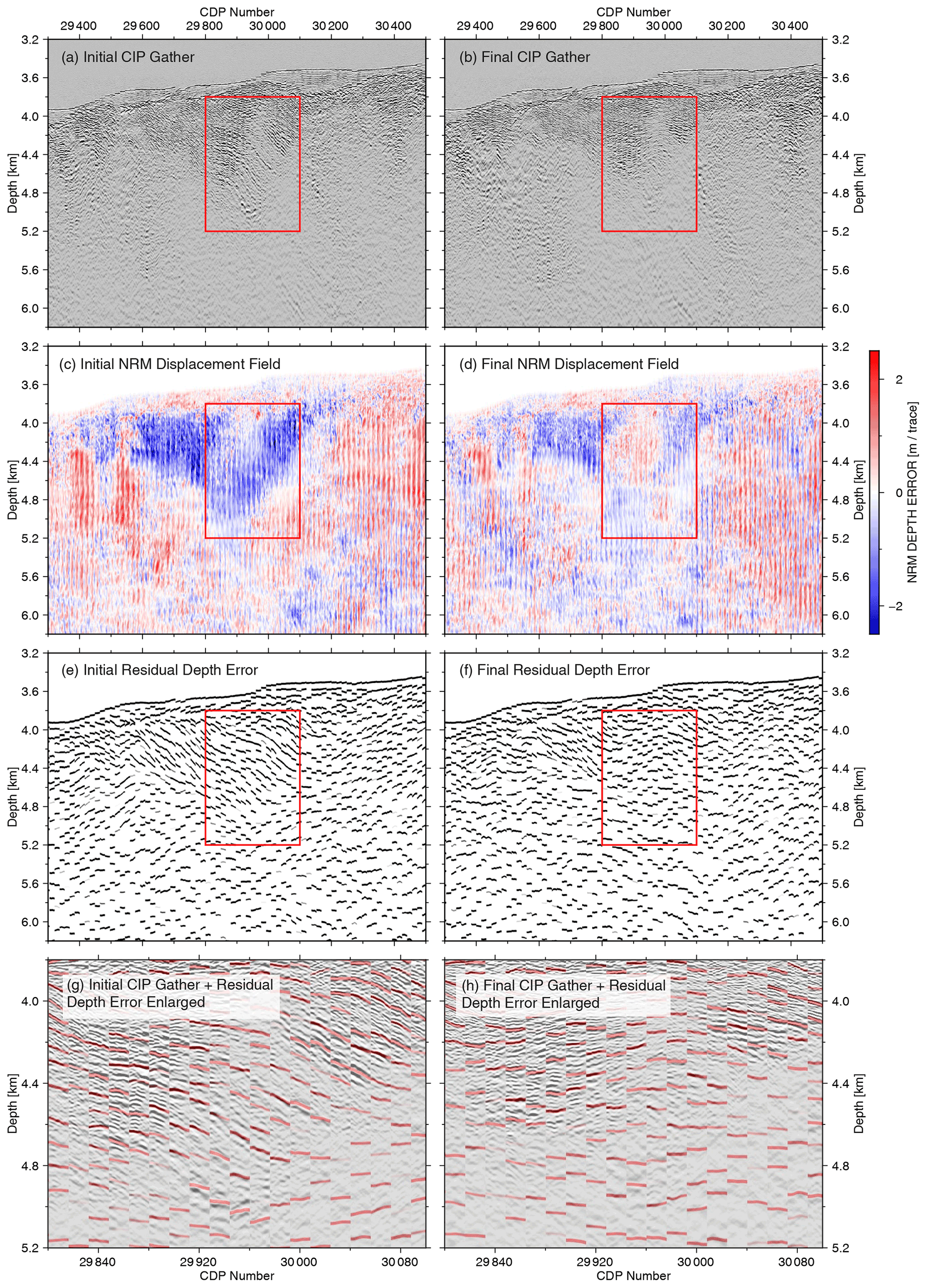
Figure 11NRM velocity update of Fig. 10 in CIP domain. (a) CIP gathers based on the initial velocity model. (b) CIP gathers based on the final velocity model. (c) Initial NRM depth shifts in the CIP domain. (d) Final NRM depth shift in CIP domain. (e) RMO picks calculated from the initial NRM displacement field. (f) RMO picks calculated from the final NRM displacement field. Note that the distinct area of velocity overestimation in the red rectangle in (c) has been substantially reduced after the tomography (d). CIP gathers (e) and (f) of the red rectangle from (c) and (d) respectively overlaid by RMO picks. Strong dipping events in the initial CIP gather (g) have mostly been flattened after the final iteration (h).
Comparing the initial and final CIP gathers in Fig. 11a and b inside the red rectangle, strong downward-dipping reflections indicate the requirement to reduce the initial velocity significantly. The NRM displacement field in Fig. 11c provides a more quantitative view of this requirement, seen by the strong blue colour with more than 2 m depth error per trace distance. The RMO picks calculated in Fig. 11e and overlain on the seismic image (Fig. 11g) follow the seismic down-dipping reflection trend quite accurately. After the tomography, the final NRM displacement is significantly reduced (Fig. 11d and f), the residual calculated depth error in the red box (Fig. 11h) is reduced, and the reflectors are in better horizontal alignment.
To the left of the red box between CDP 29 600 and 29 800, above 4.4 km depth, the tomography could only partially remove the depth error (compare Fig. 11c and d). The reflections in this region could only be aligned with velocities far below the water velocity, indicating that side echoes or cross-dipping structures in this region prevent a reliable subsurface velocity determination. To avoid such unrealistic velocity updates during the tomography, a minimum velocity of 1750 m s−1 below the seafloor was defined as a precondition.
3.6.2 Lower-slope NRM tomography
In the lower-slope region (Fig. 9a, example C), sediment layers are segmented and folded as a result of the regional compressive deformation exerted by the subduction accretion processes. The initial pre-stack depth migration example is shown in Fig. 12c. After the tomography, the final velocity increased by 500 m s−1 on average (Fig. 12b), resulting in a significant increase in the velocity gradient compared to the initial velocity model (Fig. 12a). In the final PSDM section (Fig. 12d), the reflector strength generally increased, and new reflector segments became emphasized compared to the initial migration (Fig. 12c). This is especially evident in the depth range from 6.0 to 6.8 km.
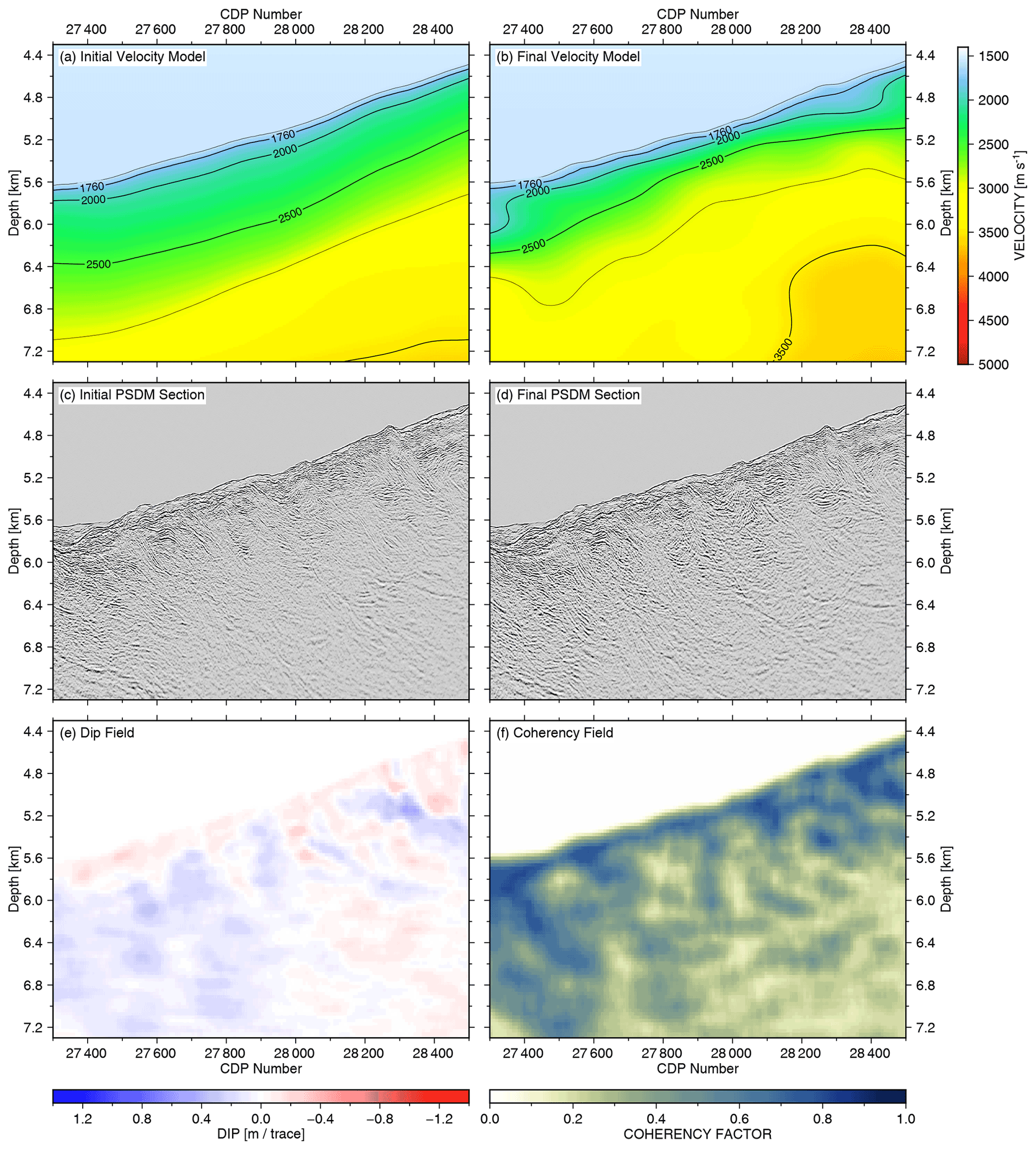
Figure 12Depth tomography example C in Figs. 5 and 9a, with CDP ranging from 27 200 to 28 600. (a) Initial velocity model merged from velocity analysis and wide-angle refraction tomography. (b) Final velocity model after six iterations of NRM-based depth tomography and PSDM. (c) PSDM result based on the initial velocity model. (d) PSDM result based on the final velocity model. (e) Reflector dip field calculated from the final PSDM result. (f) Reflector coherency field calculated from the final PSDM result. Note that the vertical velocity gradient below the seafloor increased in the final velocity model (b) compared to the initial velocity model (a) with a result of stronger focusing of reflected energy by the PSDM (d) compared to (c).
In the initial CIP gathers displayed in Fig. 13a, the reflector distribution appears largely uncorrelated, and no clear trends are visible, particularly within the red box. In the initial NRM displacement field (Fig. 13c), there is a general positive depth error character that dominates the gathers, as indicated by the red colour, especially within the red rectangle and in the initial residual depth error (Fig. 13e).
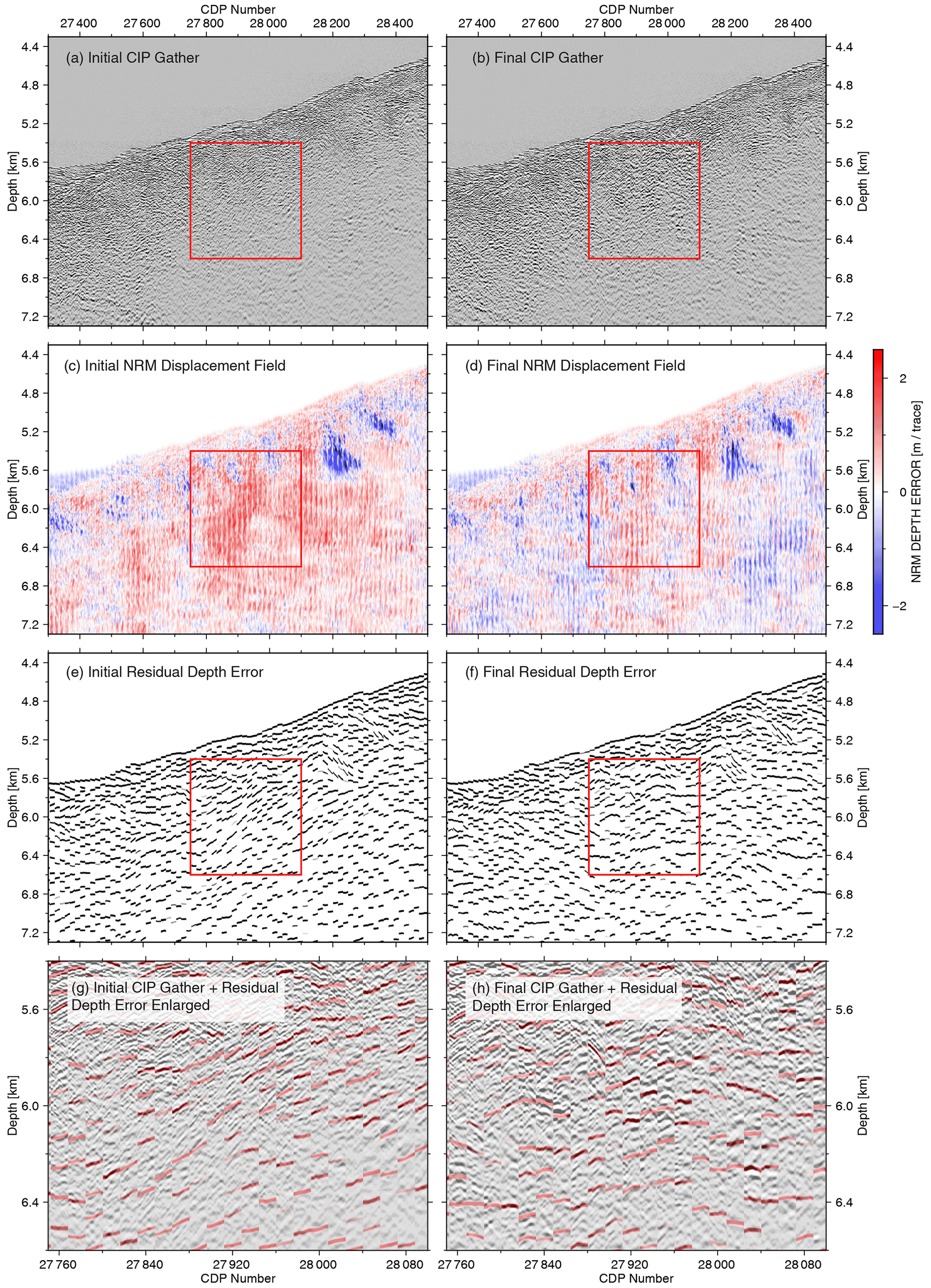
Figure 13NRM velocity updating of Fig. 12 in CIP domain. (a) CIP gathers based on the initial velocity model. (b) CIP gathers based on the final velocity model. (c) Initial NRM depth shifts in the CIP domain. (d) Final NRM depth shift in CIP domain. (e) RMO picks calculated from the initial NRM displacement field. (f) RMO picks calculated from the final NRM displacement field. Note that the distinct area of velocity underestimation in the red rectangle in (c) has been substantially decreased after the tomography (d). CIP gathers (e) and (f) of the red rectangle from (c) and (d) respectively overlaid by RMO picks. Strong dipping events in the initial CIP gather (g) have only partially flattened after the final iteration (h).
By increasing the velocities based on the tomography result, this misalignment is reduced both in the final NRM displacement field (Fig. 13d) and in the final residual depth error illustrated by the generally more horizontal alignment of the events (Fig. 13f). In the enlarged view of Fig. 13g and h, the general positive dip trend has been mostly removed. However, local reflector misalignment is still observed, as documented by the local blue colour in the NRM displacement of downward-dipping events (Fig. 13d). Even after the tomography, the two local anomalies of four neighbouring CIP gathers between CDP 28 200 and 28 400, at 5 and 5.6 km depth, were not correctly aligned. These local anomalies have a lateral dimension of ∼ 200 m and are therefore 3 times shorter than the smallest horizontal scale length smoothing used for the last iteration of the tomography (Table 3).
4.1 Final velocity model and reflectivity structure
The final depth image with the velocity model (Fig. 9) and the final subsurface velocity model (Fig. 14b) compared to the smoothed initial velocity (Fig. 14a) shows local velocity changes in the upper 3 km below the seafloor. To emphasize the differences, the percentage of change is calculated in Fig. 14c.
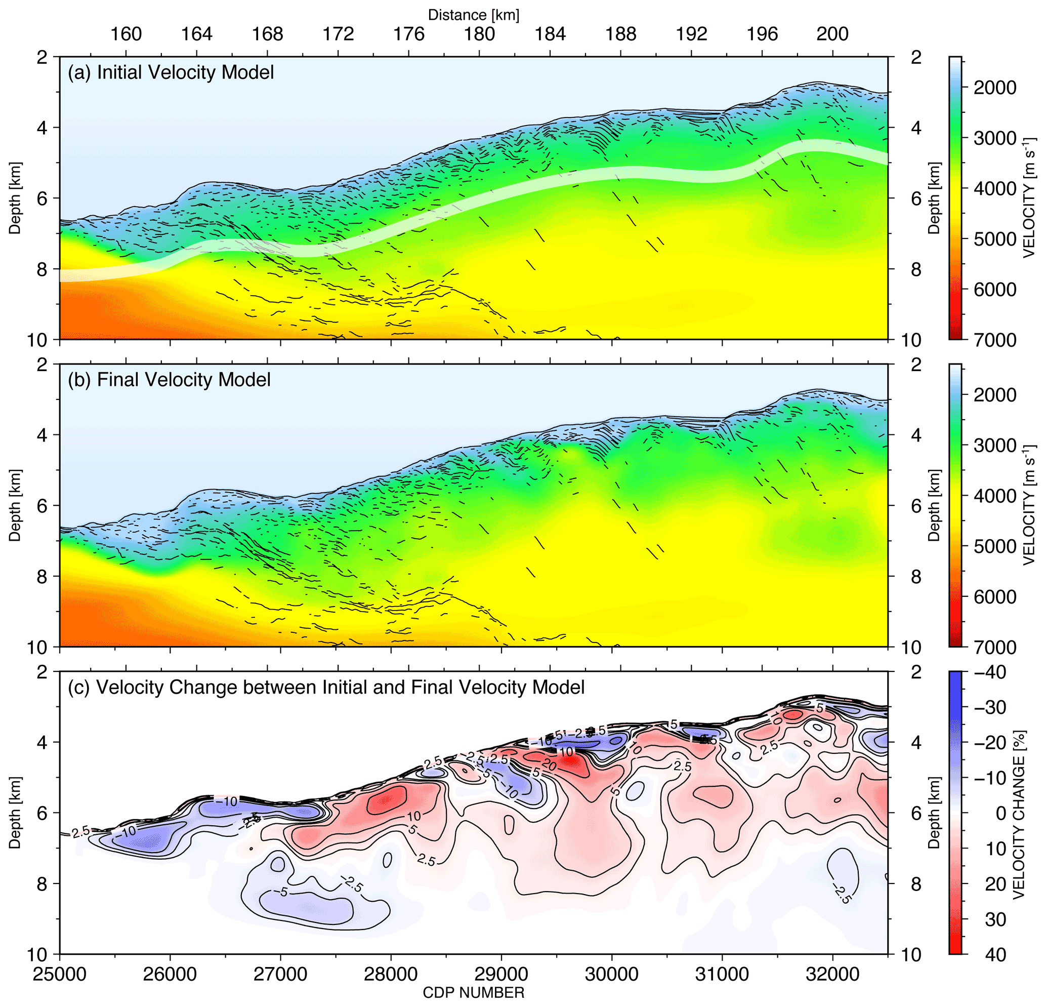
Figure 14(a) The initial velocity model merged with the wide-angle velocity model (below the white transparent band). The line drawing is based on the final PSDM image. (b) The final velocity model calculated from five iterations of the ray-based tomographic velocity inversion. (c) The velocity change in percentage from the initial to the final model.
Close to the trench axis (CDP 25 500–26 000), a velocity reduction of more than 10 % from 2100 to 1800 m s−1 is observed relative to the initial velocity (Fig. 14c). The final velocity close to this area increases from 1750 m s−1 at the seafloor to 2280 m s−1 at the plate boundary at 7400 m depth. In contrast, the uplifted sediment ridge (CDP 26 000–27 000) shows a velocity increase from 1750 to 1850 m s−1 in the upper 500 m below the seafloor, whereas the velocity increases up to 2650 m s−1 at an observed basement high at 7100 m depth.
On the lower slope (CDP 27 000–29 000) an increase in the velocity of more than 10 % compared to the initial velocity is observed and is comparable to the original OBS velocity. A thin pelagic layer of slope sediment with a maximum thickness of 100 m with velocities of 1750 m s−1 covers a highly fractured accretionary prism. The velocity below the slope sediment increases gradually in the upper 1500 m up to 3400 m s−1, which is higher than the OBS velocity model. The relatively high velocity of the major part of the accretionary wedge, which is composed of the ancient oceanic pelagic sedimentary rocks, yields long-term compaction and consolidation of the sedimentary structure. Additionally, the complex reflectivity pattern of strongly folded and fractured strata with limited spatial extents (Figs. 9a, 12d) due to compressional tectonic deformation manifests itself in small thrust ridges at the seafloor with a landward-dipping reflectivity pattern below (e.g. CDP 28 300, 28 700).
In between the dipping reflectivity patches, shallow deformed layered sediment structures with reduced velocities of 1900 m s−1 are observed with landward increasing thickness from 200 to 500 m and start to form anticline structures with the increasing spatial size and reflector continuity (CDP 28 800–29 000).
On the upper slope (CDP 29 000–32 400) the shallow reflector continuity from the lower slope increases in thickness from 500 up to 2000 m and forms continuous landward-dipping structures (Figs. 9b, 10d). The folded anticline structures (CDP 29 000–29 600) at a depth of 4 to 6 km and a sequence of thrust ridges with intervening piggyback basin (CDP 30 500–31 100, depth 3.5 to 4.5 km), as well as the landward increasing steepening of the thrust sheets, document the long-lasting compressional character of this prism.
In our final PSDM section (Fig. 9), the plate interface of the subduction zone is continuously imaged from profile kilometre 166 to kilometre 202 at a depth between 8 to 12 km. Due to the limited streamer length (3000 m) the plate interface in the deeper region is only slightly repositioned, but we did not observe a significant improvement of the reflection amplitude between the initial PSDM and the final PSDM sections. However, a different amplitude versus offset (AVO) distribution in the CIP gather along deeper reflections may be expected due to a change of the ray path bending from velocity updates in the shallow subseafloor. By using longer streamer MCS surveys, implementation of NRM grid-based reflection tomography would benefit the quantification of the plate interface reflection amplitude. This holds true especially for the AVO distribution, angle-dependent reflection coefficients, fluid budget, and its migration paths, which are related to the earthquake phenomena along the megathrust (e.g. Bangs et al., 2015; Sallarès and Ranero, 2019) and may be investigated in future studies.
4.2 Model uncertainties by tomography
In this study, we used a multi-scale length strategy for each iteration (Table 3) because a general background model existed from a wide-angle reflection and refraction tomography (Planert et al., 2010). Due to the limited streamer length, velocity updates deeper than 3 km were not expected, and the long scale-length velocity variation by the OBS model was assumed to be well resolved. Our main target in this study was the shallow subseafloor structure up to 3 km depth, which consists of spatially varying reflector size elements and varying dips. As an example, we discuss the data from the upper slope in Figs. 10 and 11 in more detail. The result of the velocity updates and the reflector alignment for each of the five iterations are shown in Fig. 15a–e. The total velocity update is the summation of the individual iteration's velocity update (Fig. 15f). By adding this velocity to the initial velocity will in general be the final velocity model.
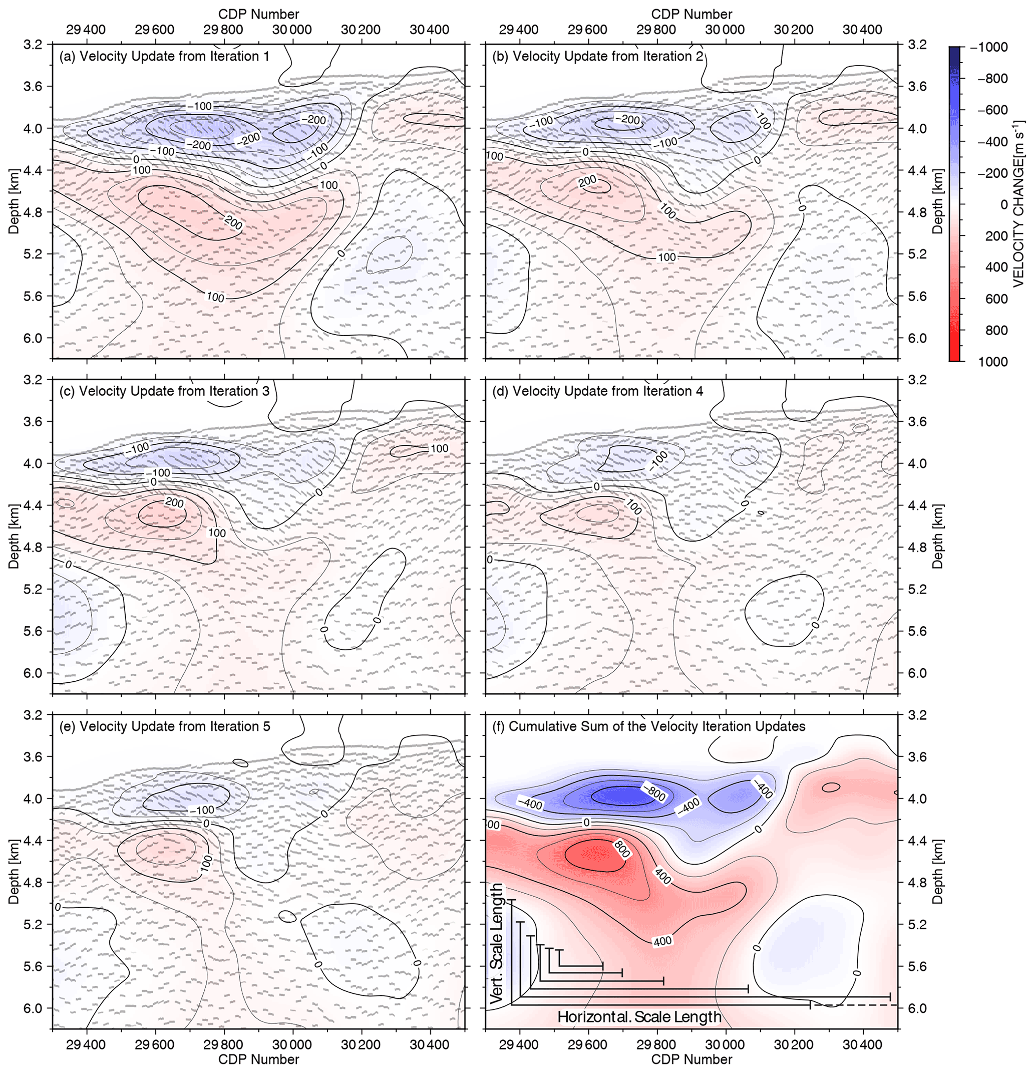
Figure 15(a–e) Velocity update after each iteration of the gridded tomography together with the CIP depth alignment after each iteration. (f) The cumulative sum of the velocity updates from all five iterations together with the horizontal and vertical smoothing length used by the scale length reductions in each iteration.
After the first iteration (Fig. 15a) a strong velocity decrease of more than 200 m s−1 at a depth of 4 km was predicted, even though the CIP gathers after this first iteration show strong misalignments. All six individual scale lengths applied sequentially for a single iteration (Table 3) are illustrated in Fig. 15f as horizontal and vertical lines. The high-velocity increase of 200 m s−1 below the velocity reduction was needed to compensate for the velocities above, especially if the CIP gather had before no misalignments. This compensation effect of the interval velocity is common in interactive CIP-gather picking. During additional iterations, the misalignment could successively be reduced (e.g. Fig. 15e), but the final velocity reached unrealistic sediment values of 1300 m s−1 due to the reduction of more than 800 m s−1 (Fig. 15f) with an initial velocity value of 2100 m s−1 at this subsurface depth. We interpreted this as an area of side echo reflections and limited the minimum velocity in this area after each iteration update by a value of 1750 m s−1. A careful critical inspection of the velocity model is needed by this purely data-driven method, but also offers the possibility to identify individual side echo reflections, which could otherwise mislead interpretations.
The smallest scale-length smoothing defined for the tomography will determine the highest possible resolution of the velocity update. To have enough redundancy at the smallest scale length, the CIP distance increment (100 m) and depth error increment (50 m) of the depth error branches were chosen so that at least seven neighbour CIP-gather and three depth error picked branches were considered. Any velocity anomalies below this scale length will not be detected. This limitation of detectable velocity anomaly can also be seen in Fig. 13d at two locations indicated by the blue colour of negative depth errors.
Due to the dense depth error information which is needed for the tomography to stabilize the linear equations (Eq. 13), manual picking is not recommended, especially if several iterations are needed. In this example of the accretionary wedge in Fig. 9 for one single iteration, 11 000 residual move-out branches were automatically picked, where each branch consists of approx. 30 individual depth picks. This number is equivalent to the number of linear equations which must be solved (Eq. 12) during the tomography.
To quantify the model uncertainties and mainly to reduce the migration computation time, new inversion strategies were developed by incorporating a Monte Carlo approach (e.g. Martin and Bell, 2019) and should be incorporated in the future. Instead of getting one final model result, multiple model results were generated based on the sensitivity and resolution of the input data for the migration. To estimate the sensitivity and resolution, which is mainly determined by the acquisition parameters and the subsurface complexity, a checkerboard test with different wavelengths and magnitudes of perturbation added to an initial velocity model will be inverted by a test tomography application. The difference to the initial model, namely the residual errors, can be used to constrain threshold values for model perturbations. The minimum spatial wavelengths and the maximum amplitude perturbation must be fulfilled for any velocity perturbation created randomly for a Monte Carlo simulation, but this analysis will not avoid the detection of side echo velocity anomalies.
To analyse model perturbations independently of the migration velocity, CIP-gather depth errors are de-migrated with their migration velocity. In the model domain, random perturbed populations of velocity input functions are generated, inverted, and updated to the input velocity model to create a possible velocity model. All these populations of velocity models of the inversions can be statistically analysed, averaged, and used for the next iteration of a migration. By analysing the cumulative depth error of the CIP gathers after the migration iterations, convergence to a predefined obtained minimum depth error can be used to stop the inversion process automatically (Martin and Bell, 2019).
4.3 Anisotropic tomography
The wave propagation, namely direction and speed, is strongly influenced by the rock type and is generally depth and azimuth dependent. A fluid-filled orientation of fractures or microcracks can cause anisotropy as well as a preferred orientation of minerals in the deeper crust. There exist several classes of symmetry for anisotropy. But for imaging and inversion often a simple transverse isotropic type with one axis of symmetry is assumed. The symmetry axis can be vertical (VTI), tilted (TTI), or horizontal (HTI). For a weakly anisotropic medium of acoustic waves, the dimensionless Thomsen parameters ε and δ are used to describe the ratio of the velocity variations (Thomsen, 1986).
Complementary datasets like in this study of near-vertical reflections and wide-angle reflection and refractions with more horizontally propagating events offer one possibility to estimate the anisotropic parameters in the illuminated subsurface areas of both datasets. Classical modelling methods are nowadays replaced by inversion strategies due to the constant growth of observation density and increasing computational power. Several developments for weak anisotropy are published, e.g. 3-D joint refraction and reflection tomography (Meléndez et al., 2019) or a ray-based gridded tomography for tilted TI media based on depth alignment of CIP gather (Wang and Tsvankin, 2011).
The ray-based gridded tomography (Eqs. 12–15) together with the non-hyperbolic NRM event tracking and picking can also be used to invert for the anisotropic parameters, e.g. ε or δ. Based on an isotropic velocity and one Thomson parameter, e.g. ε an initial anisotropic migration will be analysed in the CIP domain and a depth error estimated. Instead of calculating a change in travel time, corresponding to a change of velocity (Eqs. 12–14), the calculation is modified to a change of the Thompson parameter . By exchanging Δα to Δε and solving Eq. (15), any CIP depth error is corrected due to a change of the parameter ε. An application to real data can be found in Woodward et al. (2008). The initial isotropic velocity should be ideally a velocity depth profile corresponding to a vertical seismic profile (VSP) at each location. To overcome this limitation a significant scale length smoothing S (Eq. 15) needs to be applied as shown by Wang and Tsvankin (2011).
In the Java trench dataset, where near-vertical and wide-angle and refracted OBS data both exist, a combined analysis is limited to the move-out sensitivity by the streamer length 3–4 km below the seafloor. Additionally, both profiles do not completely coincide especially at the lower slope. The OBS model does not show significant velocity variations along the slope, especially not in the gravitationally driven slump area close to the trench axis. Instead, only a thin low-velocity layer with constant thickness is observed along the accretionary wedge (Fig. 6a). The data gap of OBS positions in the trench axis and the lack of local sediment basin incorporated into the initial wide-angle tomography model (Planert et al., 2010) have reduced the model reliability for further anisotropic analysis in the shallow illuminated area of both datasets.
The presented case study shows that CIP depth error estimations by depth warping in combination with a ray-based reflection tomography can improve depth-migrated images from MCS data. The non-rigid warping method provides reliable displacement fields for non-hyperbolic CIP depth errors. A semblance-based event tracking through the displacement field is limited by interfering reflected events. Due to the purely data-driven method of densely sampled depth error information (horizontal distance 100 m, vertical distance 50 m) more detailed spatial information for velocity corrections is available. In combination with a grid-based tomography, where depth errors are compensated for by velocity changes, the inversion from long to short lengths iteratively reduces the depth errors and improves the migration image. We suggest that further developments by integrating statistical analysis of the velocity updates (e.g. the Monte Carlo approach) and extending the tomography for anisotropic parameters will provide new analysis tools for the subsurface image within the limits of ray-based methods.
Codes used to implement the depth-variant displacement correction and residual move-out (RMO) auto-tracking on the synthetic seismic section by using the NRM method are available at https://doi.org/10.5281/zenodo.5998288 (Xia et al., 2022).
The raw and final results are available upon reasonable request.
YX and DK performed the computations and are responsible for the majority of the processing. HK helped to strengthen the overall scope and added to interpretational aspects and the discussion of the presented results. MS made the data available and was responsible for the navigation and geometry processing. YX wrote the article, and all authors contributed equally to the proofreading and final preparation of the paper.
The contact author has declared that neither they nor their co-authors have any competing interests.
Publisher’s note: Copernicus Publications remains neutral with regard to jurisdictional claims in published maps and institutional affiliations.
R/V SONNE cruise SO190 and the SINDBAD project were funded by the German Federal Ministry of Education and Research (BMBF) under grants 03G0190A and 03G0190B. Yueyang Xia acknowledges funding from the China Scholarship Council (grant 201506400067). Bathymetric data from R/V SONNE cruise SO190 can be requested through the German Bundesamt für Seeschifffahrt und Hydrographie (BSH; http://www.bsh.de, last access: 25 October 2021). Seismic reflection line SO190 BGR06-313 is stored at the Bundesanstalt für Geowissenschaften und Rohstoffe (BGR) and can be requested through the Geo-Seas data portal (https://geoseas.bgr.de/bgrwebapp/SO190/BGR06-313_mig_oem.xml, last access: 1 November 2021). The seismic data were processed with Schlumberger's Omega2 seismic processing suite OMEGA; ObsPy, a Python framework for seismology; and Seismic Unix, an open-source software package for seismic research and processing from the Center for Wave Phenomena, Colorado School of Mines. Bathymetry and seismic images are plotted by the Generic Mapping Tools (GMT) and Matplotlib. We thank Nathan L. Bangs and César R. Ranero for insightful comments and suggestions that helped to improve the paper.
R/V SONNE cruise SO190 and the SINDBAD project were funded by the German Federal
Ministry of Education and Research (BMBF) under grant nos. 03G0190A and
03G0190B. Yueyang Xia acknowledges funding from the China Scholarship Council
(grant no. 201506400067).
The article processing charges for this open-access publication were covered by the GEOMAR Helmholtz Centre for Ocean Research Kiel.
This paper was edited by Charlotte Krawczyk and reviewed by Nathan Bangs and César R. Ranero.
Aarre, V.: On the presence, and possible causes, of apparent lateral shifts below the Norne reservoir, 78th Soc. Explor. Geophys. Int. Expo. Annu. Meet. SEG 2008 Las Vegas, 3174–3178, https://doi.org/10.1190/1.3064005, 2008.
Audebert, F. and Diet, J.-P.: A focus on focusing, in: Migration I, Prestack Depth Migration and Velocity Model Building, edited by: Jones, I. F., Bloor, R. I., Boindi, B. L., and Etgen, T., Vol. 25, https://doi.org/10.1190/1.9781560801917, 2008.
Audebert, F., Diet, J.-P., Guillaume, P., Jones, I. F., and Zhang, X.: CRP-Scans: 3D PreSDM velocity analysis via zero-offset tomographic inversion, in: SEG Technical Program Expanded Abstracts 1997, Dallas, Texas, USA, 1805–1808, Society of Exploration Geophysicists, https://doi.org/10.1190/1.1885786, 1997.
Bangs, N. L., McIntosh, K. D., Silver, E. A., Kluesner, J. W., and Ranero, C. R.: Fluid accumulation along the Costa Rica subduction thrust and development of the seismogenic zone, J. Geophys. Res.-Sol. Ea., 120, 67–86, https://doi.org/10.1002/2014JB011265, 2015.
Bishop, T. N., Bube, K. P., Cutler, R. T., Langan, R. T., Love, P. L., Resnick, J. R., Shuey, R. T., Spindler, D. A., and Wyld, H. W.: Tomographic determination of velocity and depth in laterally varying media, Geophysics, 50, 903–923, https://doi.org/10.1190/1.1441970, 1985.
Claerbout, J. F.: Earth soundings analysis: Processing versus inversion, edited by: Heydron, J., Blackwell Scientific Publications London, http://sepwww.stanford.edu/sep/prof/pvi.pdf (last access: 15 February 2022), 1992.
Collot, J. Y., Ribodetti, A., Agudelo, W., and Sage, F.: The South Ecuador subduction channel: Evidence for a dynamic mega-shear zone from 2D fine-scale seismic reflection imaging and implications for material transfer, J. Geophys. Res.-Sol. Ea., 116, 1–20, https://doi.org/10.1029/2011JB008429, 2011.
Crutchley, G. J., Klaeschen, D., Henrys, S. A., Pecher, I. A., Mountjoy, J. J., and Woelz, S.: Subducted sediments, upper-plate deformation and dewatering at New Zealand's southern Hikurangi subduction margin, Earth Planet. Sc. Lett., 530, 115945, https://doi.org/10.1016/j.epsl.2019.115945, 2020.
Dix, C. H.: Seismic velocities from surface measurements, Geophysics, 20, 68–86, 1955.
Fomel, S.: Applications of plane-wave destruction filters, Geophysics, 67, 1946–1960, 2002.
Fruehn, J., Jones, I. F., Valler, V., Sangvai, P., Biswal, A., and Mathur, M.: Resolving near-seabed velocity anomalies: Deep water offshore eastern India, Geophysics, 73, VE235–VE241, https://doi.org/10.1190/1.2957947, 2008.
GEBCO Bathymetric Compilation Group 2020: The GEBCO_2020 Grid – a continuous terrain model of the global oceans and land, British Oceanographic Data Centre, National Oceanography Centre [data set], NERC, UK, https://doi.org/10/dtg3, 2020.
Górszczyk, A., Operto, S., Schenini, L., and Yamada, Y.: Crustal-scale depth imaging via joint full-waveform inversion of ocean-bottom seismometer data and pre-stack depth migration of multichannel seismic data: a case study from the eastern Nankai Trough, Solid Earth, 10, 765–784, https://doi.org/10.5194/se-10-765-2019, 2019.
Gras, C., Dagnino, D., Jiménez-Tejero, C. E., Meléndez, A., Sallarès, V., and Ranero, C. R.: Full-waveform inversion of short-offset, band-limited seismic data in the Alboran Basin (SE Iberia), Solid Earth, 10, 1833–1855, https://doi.org/10.5194/se-10-1833-2019, 2019.
Guitton, A. and Verschuur, D. J.: Adaptive subtraction of multiples using the L1-norm, Geophys. Prospect., 52, 27–38, 2004.
Hale, D.: A method for estimating apparent displacement vectors from time-lapse seismic images, Geophysics, 74, V99–V107, https://doi.org/10.1190/1.3184015, 2009.
Hale, D.: Dynamic warping of seismic images, Geophysics, 78, S105–S115, https://doi.org/10.1190/GEO2012-0327.1, 2013.
Hall, S. A.: A methodology for 7D warping and deformation monitoring using time-lapse seismic data, Geophysics, 71, O21, https://doi.org/10.1190/1.2212227, 2006.
Hampson, D.: Inverse velocity stacking for multiple elimination, J. Can. Soc. Explor. Geophys., 22, 44–55, 1986.
Han, S., Bangs, N. L., Carbotte, S. M., Saffer, D. M., and Gibson, J. C.: Links between sediment consolidation and Cascadia megathrust slip behaviour, Nat. Geosci., 10, 954–959, https://doi.org/10.1038/s41561-017-0007-2, 2017.
Hardy, P.: High resolution tomographic MVA with automation, in: 66th EAGE Conference & Exhibition, Paris, 2004, p. cp-133, https://doi.org/10.3997/2214-4609.201405668, 2003.
Horn, B. K. P. and Schunck, B. G.: Determining optical flow, Artif. Intell., 17, 185–203, https://doi.org/10.1016/0004-3702(81)90024-2, 1981.
Jones, I. F.: A review of 3D PreSDM model building techniques, First Break, 21, https://doi.org/10.3997/1365-2397.21.3.25408, 2003.
Jones, I. F.: Tutorial: Velocity estimation via ray-based tomography, First Break, 28, 45–52, 2010.
Jones, I. F., Sugrue, M. J., and Hardy, P. B.: Hybrid Gridded Tomography, First Break, 25, https://doi.org/10.3997/1365-2397.2007013, 2007.
Jones, I. F., Ibbotson, K., Grimshaw, M., and Plasterie, P.: Prestack Depth Migration and Velocity Model Building, edited by: Jones, I. F., Bloor, R. I., Biondi, B. L., and Etgen, J. T., Society of Exploration Geophysicists, https://doi.org/10.1190/1.9781560801917, 2008.
Kosloff, D., Sherwood, J., Koren, Z., Machet, E., and Falkovitz, Y.: Velocity and interface depth determination by tomography of depth migrated gathers, Geophysics, 61, 1511–1523, 1996.
Levitus, S.: Climatological Atlas of the World Ocean, EOS T. Am. Geophys. Un., 64, 962–963, https://doi.org/10.1029/EO064i049p00962-02, 1983.
Li, J., Shillington, D. J., Saffer, D. M., Bécel, A., Nedimović, M. R., Kuehn, H., Webb, S. C., Keranen, K. M., and Abers, G. A.: Connections between subducted sediment, pore-fluid pressure, and earthquake behavior along the Alaska megathrust, Geology, 46, 299–302, https://doi.org/10.1130/G39557.1, 2018.
Lüschen, E., Müller, C., Kopp, H., Engels, M., Lutz, R., Planert, L., Shulgin, A., Djajadihardja, Y. S., Lueschen, E., Mueller, C., Kopp, H., Engels, M., Lutz, R., Planert, L., Shulgin, A., and Djajadihardja, Y. S.: Structure, evolution and tectonic activity of the eastern Sunda forearc, Indonesia, from marine seismic investigations, Tectonophysics, 508, 6–21, https://doi.org/10.1016/j.tecto.2010.06.008, 2011.
MacKay, S. and Abma, R.: Imaging and velocity estimation with depth-focusing analysis, Geophysics, 57, 1608–1622, 1992.
Martin, T. and Bell, M.: An innovative approach to automation for velocity model building, First Break, 37, 57–65, https://doi.org/10.3997/1365-2397.n0033, 2019.
Meléndez, A., Jiménez, C. E., Sallarès, V., and Ranero, C. R.: Anisotropic P-wave travel-time tomography implementing Thomsen's weak approximation in TOMO3D, Solid Earth, 10, 1857–1876, https://doi.org/10.5194/se-10-1857-2019, 2019
Neidell, N. S. and Taner, M. T.: Semblance and other coherency measures for multichannel data, Geophysics, 36, 482–497, 1971.
Nickel, M., Sønneland, L., and Geco-prakla, S.: Non-rigid matching of migrated time-lapse seismic SEG 1999 Expanded Abstracts SEG 1999 Expanded Abstracts, Houston, Texas, USA, https://doi.org/10.1190/1.1821191, 1999.
Pappu, S., Gold, S., and Rangarajan, A.: A framework for nonrigid matching and correspondence, edited by: Touretzky, D. S., Mozer, M. C., and Hasselmo, M. E., Advances in Neural Information Processing Systems, 8, MIT Press, Cambridge, MA, 1996.
Perez, G. and Marfurt, K. J.: Warping prestack imaged data to improve stack quality and resolution, Geophysics, 73, 1–7, https://doi.org/10.1190/1.2829986, 2008.
Planert, L., Kopp, H., Lüschen, E., Mueller, C., Flueh, E. R., Shulgin, A., Djajadihardja, Y., and Krabbenhoeft, A.: Lower plate structure and upper plate deformational segmentation at the Sunda-Banda arc transition, Indonesia, J. Geophys. Res.-Sol. Ea., 115, 1–25, https://doi.org/10.1029/2009JB006713, 2010.
Reiche, S. and Berkels, B.: Automated stacking of seismic reflection data based on nonrigid image matching, Geophysics, 83, V171–V183, https://doi.org/10.1190/geo2017-0189.1, 2018.
Rickett, J. E. and Lumley, D. E.: Cross-equalization data processing for time-lapse seismic reservoir monitoring: A case study from the Gulf of Mexico, Geophysics, 66, 1015–1025, 2001.
Riedel, M., Reiche, S., Aßhoff, K., and Buske, S.: Seismic depth imaging of sequence boundaries beneath the New Jersey shelf, Mar. Geophys. Res., 40, 17–32, https://doi.org/10.1007/s11001-018-9360-9, 2019.
Robinson, E. A. and Treitel, S.: Geophysical signal analysis, Society of Exploration Geophysicists, https://doi.org/10.1190/1.9781560802327, 2000.
Sallarès, V. and Ranero, C. R.: Upper-plate rigidity determines depth-varying rupture behaviour of megathrust earthquakes, Nature, 576, 96–101, https://doi.org/10.1038/s41586-019-1784-0, 2019.
Shiraishi, K., Moore, G. F., Yamada, Y., Kinoshita, M., Sanada, Y., and Kimura, G.: Seismogenic zone structures revealed by improved 3-D seismic images in the Nankai Trough off Kumano, Geochem. Geophy. Geosy., 20, 2252–2271, 2019.
Sripanich, Y., Fomel, S., Trampert, J., Burnett, W., and Hess, T.: Probabilistic moveout analysis by time warping, Geophysics, 85, U1–U20, https://doi.org/10.1190/geo2018-0797.1, 2020.
Stork, C.: Reflection tomography in the postmigrated domain, Geophysics, 57, 680–692, https://doi.org/10.1190/1.1443282, 1992.
Sugrue, M., Jones, I. F., Evans, E., Fairhead, S., and Marsden, G.: Enhanced velocity estimation using gridded tomography in complex chalk, Geophys. Prospect., 52, 683–691, 2004.
Thomsen, L.: Weak elastic anisotropy, Geophysics, 51, 1954–1966, https://doi.org/10.1190/1.1442051, 1986.
Tomar, G., Singh, S. C., and Montagner, J.-P.: Sub-sample time shift and horizontal displacement measurements using phase-correlation method in time-lapse seismic, Geophys. Prospect., 65, 407–425, 2017.
Van Trier, J. A.: Tomographic determination of structural velocities from depth-migrated seismic data, thesis, Stanford University, http://sepwww.stanford.edu/data/media/public/oldreports/sep66/66_00.pdf (last access: 15 February 2022), 1990.
Verschuur, D. J., Berkhout, A. J., and Wapenaar, C. P. A.: Adaptive surface-related multiple elimination, Geophysics, 57, 1166–1177, https://doi.org/10.1190/1.1443330, 1992.
Wang, X. and Tsvankin, I.: Ray-based gridded tomography for tilted TI media, in: SEG Technical Program Expanded Abstracts 2011, San Antonio, Texas, USA, 237–242, Society of Exploration Geophysicists, https://doi.org/10.1190/1.3627687, 2011.
Wolberg, G.: Digital image warping, IEEE computer Society Press Los Alamitos, CA, ISBN: 978-08-1868-944-4, 1990.
Woodward, M. J., Nichols, D., Zdraveva, O., Whitfield, P., and Johns, T.: A decade of tomography, Geophysics, 73, VE5, https://doi.org/10.1190/1.2969907, 2008.
Xia, Y., Klaeschen, D., Kopp, H., and Schnabel, M.: Supplementary code for article “Reflection tomography by depth warping: A case study across the Java trench” on Solid Earth (SE-2021-40), Zenodo [code], https://doi.org/10.5281/zenodo.5998288, 2022.
Xue, Z., Zhang, H., Zhao, Y., and Fomel, S.: Pattern-guided dip estimation with plane-wave destruction filters, Geophys. Prospect., 67, 1798–1810, 2019.
Yilmaz, Ö.: Seismic data analysis: Processing, inversion, and interpretation of seismic data, Society of exploration geophysicists, https://doi.org/10.1190/1.9781560801580, 2001.
Zhang, D., Wang, X., Huang, Y., and Schuster, G.: Warping for trim statics, in: SEG Technical Program Expanded Abstracts 2014, Denver, Colorado, USA, 3946–3950, Society of Exploration Geophysicists, https://doi.org/10.1190/segam2014-0281.1, 2014.
- Abstract
- Introduction
- Method: non-rigid matching and reflection tomography
- Application of a reflection tomography by CIP residual move-out warping across the Java trench
- Discussion
- Conclusions
- Code availability
- Data availability
- Author contributions
- Competing interests
- Disclaimer
- Acknowledgements
- Financial support
- Review statement
- References