the Creative Commons Attribution 4.0 License.
the Creative Commons Attribution 4.0 License.
 | 17 May 2022
Three-dimensional reflection seismic imaging of the iron oxide deposits in the Ludvika mining area, Sweden, using Fresnel volume migration
Felix Hloušek
Michal Malinowski
Lena Bräunig
Stefan Buske
Alireza Malehmir
Magdalena Markovic
Lukasz Sito
Paul Marsden
Emma Bäckström
We present pre-stack depth-imaging results for a case study of 3D reflection seismic exploration at the Blötberget iron oxide mining site belonging to the Bergslagen mineral district in central Sweden. The goal of the study is to directly image the ore-bearing horizons and to delineate their possible depth extension below depths known from existing boreholes. For this purpose, we applied a tailored pre-processing workflow and two different seismic imaging approaches, Kirchhoff pre-stack depth migration (KPSDM) and Fresnel volume migration (FVM). Both imaging techniques deliver a well-resolved 3D image of the deposit and its host rock, where the FVM image yields a significantly better image quality compared to the KPSDM image. We were able to unravel distinct horizons, which are linked to known mineralization and provide insights on their possible lateral and depth extent. Comparison of the known mineralization with the final FVM reflection volume suggests a good agreement of the position and the shape of the imaged reflectors caused by the mineralization. Furthermore, the images show additional reflectors below the mineralization and reflectors with opposite dips. One of these reflectors is interpreted to be a fault intersecting the mineralization, which can be traced to the surface and linked to a fault trace in the geological map. The depth-imaging results can serve as the basis for further investigations, drilling, and follow-up mine planning at the Blötberget mining site..
- Article
(13527 KB) - Full-text XML
- BibTeX
- EndNote


In the last few decades the need for raw materials has increased worldwide (e.g., Dubiński, 2013, and references therein; Paulick and Nurmi, 2018). This increasing demand also accounts for the European Union (EU). However, in contrast to this demand, current exploration and mining activities and the development of new mineral resources is still on a low level. Several mines were abandoned between the 1960s and 1980s as mining in Europe was too expensive (e.g., Crowson, 1996; Berverksstatistik, 2013) and global prices were constantly falling. In recent years, the EU has aimed to reactivate activities related to the exploration and production of critical minerals, with a special focus on the so-called critical raw materials (e.g., Malehmir et al., 2012, 2020). In that context, a reliable and cost-effective exploration of such minerals is an important step in the early stage of the whole raw materials value chain. Therefore, the EU has supported several projects that focus on the improvement of this exploration stage, e.g., through the EU-funded Smart Exploration™ project (Mahlemir et al., 2019), which had the primary goal of creating and improving new approaches for mineral exploration using geophysical methods.
Seismic methods play an important role in mineral exploration (Eaton et al., 2003a, b). They have the potential to allow for a high-resolution characterization of mineral deposits at depth. Reflection seismic surveys in particular can yield a structural image of potential deposits, their host rocks, and other geological structures related to the understanding of their genesis, such as faults and fracture systems. However, reflection seismic methods in mineral exploration are not yet as well established as they are in hydrocarbon exploration (L'Heureux et al., 2005). Their application is often challenged by the corresponding hard-rock environment causing strong scattering of the seismic wavefield and by complex 3D structures, since the geological units can show strongly varying strike and dip directions that may intersect each other. Furthermore, the expectable signal-to-noise ratio is rather low due to low impedance contrasts and strong scattering attenuation. Additionally, typical land seismic issues, such as irregular source and receiver spacing, often poor source and receiver coupling, topographic effects, and strong near-surface velocity gradients must be considered during seismic data processing.
Despite these challenges, reflection seismic imaging has started to gain increased popularity for use in mineral exploration (Malehmir et al., 2012). Several studies have shown the potential of 2D and 3D reflection seismic investigations for such mineral exploration (e.g., Milkereit, et al., 1996; Urosevic et al., 2012; Cheraghi et al., 2012; Malehmir et al., 2012, and references therein; Bellefleur et al., 2015), but methodological improvements are still needed on the seismic imaging side, especially in cases with complex subsurface structures and irregular acquisition geometries, which are typical for seismic surveys in populated areas due to environmental and accessibility issues.
The work presented in this paper has been performed as part of the Smart Exploration™ project and focuses on imaging mineral resources using reflection seismic methods with a special focus on pre-stack depth-imaging techniques. We showcase this approach for an investigation area located in the Bergslagen mining district in central Sweden (Fig. 1). The deposit itself consists mainly of magnetite and hematite, which occurs in 30–50 m thick sheet-like bodies dipping towards the southeast to around 850 m depth (Maries et al., 2017; Malehmir et al., 2017). The 2D reflection seismic profiles had already been acquired during 2015 and 2016 and cross the known mineralization perpendicular to its main strike direction. The combined dataset was successfully processed using a standard time domain processing and post-stack imaging workflow (Markovic et al., 2020), Kirchhoff pre-stack depth migration (KPSDM), and advanced imaging approaches based on KPSDM (Bräunig et al., 2019). The results of these 2D surveys show a clear image of the expected mineralized bodies and their surrounding structures at depth. The obtained seismic images show that the known mineralization likely extends deeper than previously known from borehole investigations. The images also show internal structures (e.g., faults causing vertical offsets) within the lateral extent of the reflectors. Furthermore, several reflectors with an opposite dip direction were mapped in the reflection seismic images. In particular, one of these reflectors is of greater interest, since it apparently marks the lowermost end of the deposits. However, in order to reveal the true 3D structure and to better evaluate the potential resources, a sparse 3D seismic survey was conducted in April–May 2019. The results of a conventional post-stack time migration workflow were shown in Malehmir et al. (2021). Here, we present the corresponding results of a pre-stack depth-imaging workflow applied to the same dataset in order to provide further support and improved images of the subsurface, and we also show the potential of depth-imaging algorithms for such a dataset and level of geological complexity.
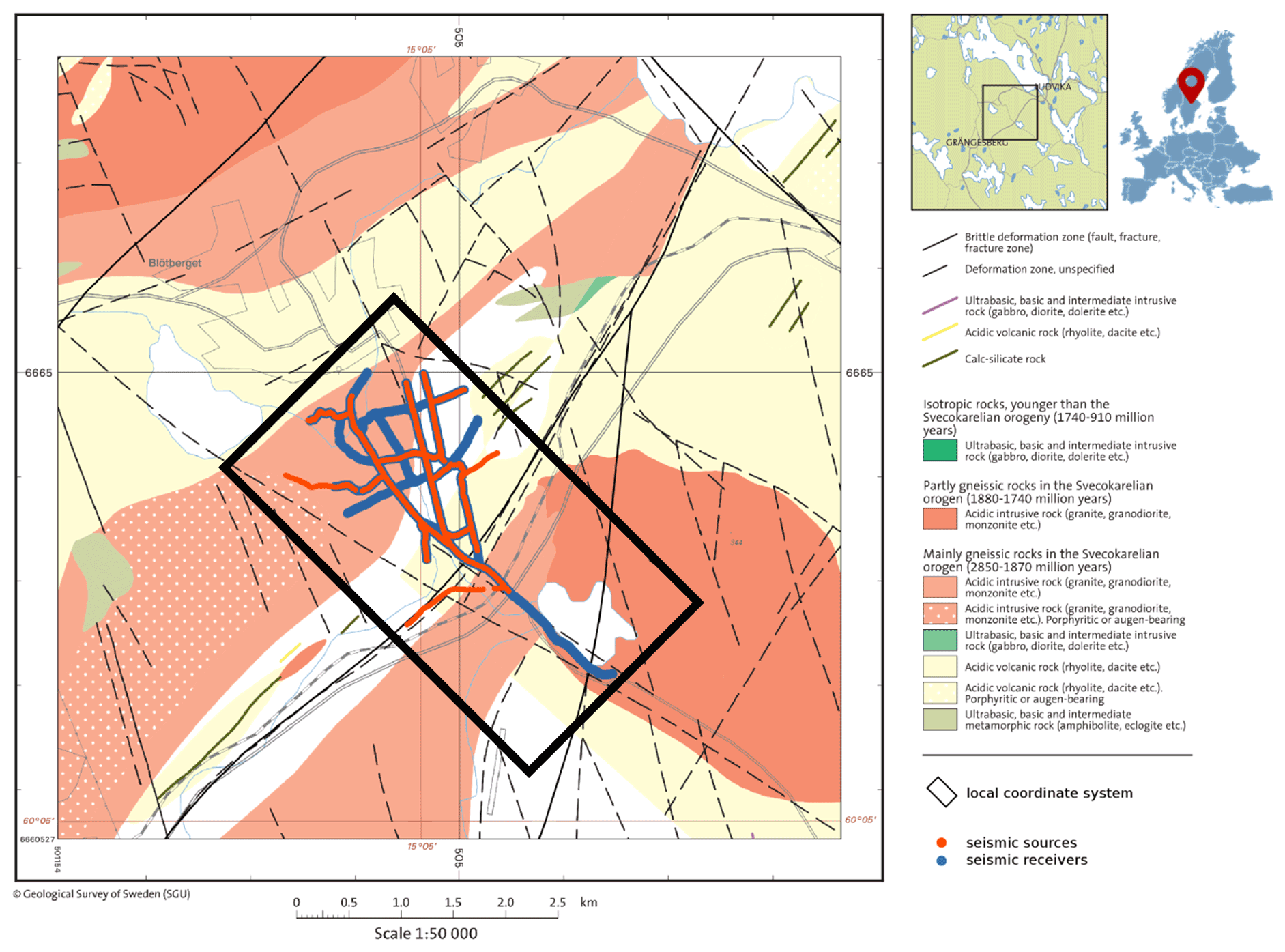
Figure 1Geological map and survey layout with source (red) and receiver (blue) positions of the 3D survey and the local coordinate system used for first-break travel time tomography and depth imaging (black box). Courtesy of the Geological Survey of Sweden.
For the previously acquired 2D seismic data, Bräunig et al. (2019) demonstrated a suitable imaging workflow with pre-stack depth migration as the last step resulting in a final depth image. Furthermore, they showed that the application of focusing pre-stack depth migration techniques, such as Fresnel volume migration (FVM) (Lüth et al., 2005; Buske et al., 2009), coherency migration (Hloušek et al., 2015a), or coherency-based FVM (Hloušek et al., 2015b) can improve the resulting image of the mineralization for the 2D dataset and therefore allows for a more detailed interpretation compared to a simple KPSDM approach. Following these promising results, we also applied the FVM approach to the new 3D dataset and compare it to the result of a basic KPSDM. The migration is guided by a careful pre-processing sequence, including static corrections, and by a reasonable choice of a migration velocity model.
The 3D seismic data were acquired over the Blötberget iron oxide deposit of the Ludvika mines in central Sweden (Fig. 1). The area belongs to the Bergslagen mineral-endowed district, which hosts a significant amount of iron oxide and sulfide deposits. It is historically well known because of its importance in the historical mining industry (Stephens et al., 2009). In Blötberget, the deposits were mined until 1979 down to a level of 280–360 m (Malehmir et al., 2021). Several historical and newly drilled boreholes investigated the mineralization, mainly at depths between 300 and 600 m (Maries et al., 2017). Borehole logs have shown that the mean P-wave bedrock velocity varies between 5500 and 6000 m s−1. The P-wave velocity of the main mineralization is in the same range and shows only some small outliers with slightly higher velocities (Fig. 2). Nevertheless, the main mineralization can be expected to be reflective, since the density log shows a strong increase in density for the mineralized zones, and hence a potential increase in acoustic impedance from the host bedrock to the mineralization can be seen.
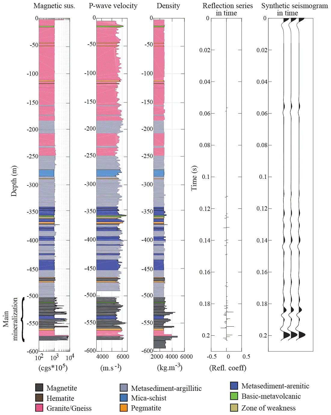
Figure 2Downhole geophysical logs, theoretical reflection coefficients, and synthetic seismograms from the host rock and the main mineralization (from Maries et al., 2017).
The deposits are situated within volcano-sedimentary rocks of the Paleoproterozoic age (1.85–1.8 Ga), which are typically overprinted by various degrees of metamorphism. More than 40 % of the iron ore produced are from apatite-rich iron oxide deposits (Allen et al., 1996; Magnusson 1970) and are considered to have a magmatic–hydrothermal origin (Jonsson et al., 2013). The Blötberget area in particular is known for its high-quality iron oxide apatite-bearing mineralization. More than 50 % of the iron is hosted in magnetite and sometimes hematite horizons. Hematite deposits are less massive and their skarn host rock contains more quartz and feldspar. The mineralized bodies are intersected by mafic dikes and subvolcanic intrusions (Pertuz et al., 2021),
The typical sheet-like mineralization occurs at different levels. At Blötberget, two dominant apatite-rich mineralized bodies dip to the southeast at an angle of 45 ∘ down to a depth of 500 m (Fig. 3). Below that they continue with a slightly shallower dip down to a known depth of 800–850 m (Malehmir et al., 2017). No borehole data below 800 m are available, and information on the lateral extent is missing. Therefore, interpretation using the newly acquired 3D seismic dataset proves the validity of the depth extension of the mineralization conducted in the former seismic surveys and focuses on the lateral extent of the mineralization, the surrounding structures, and their further characterization.
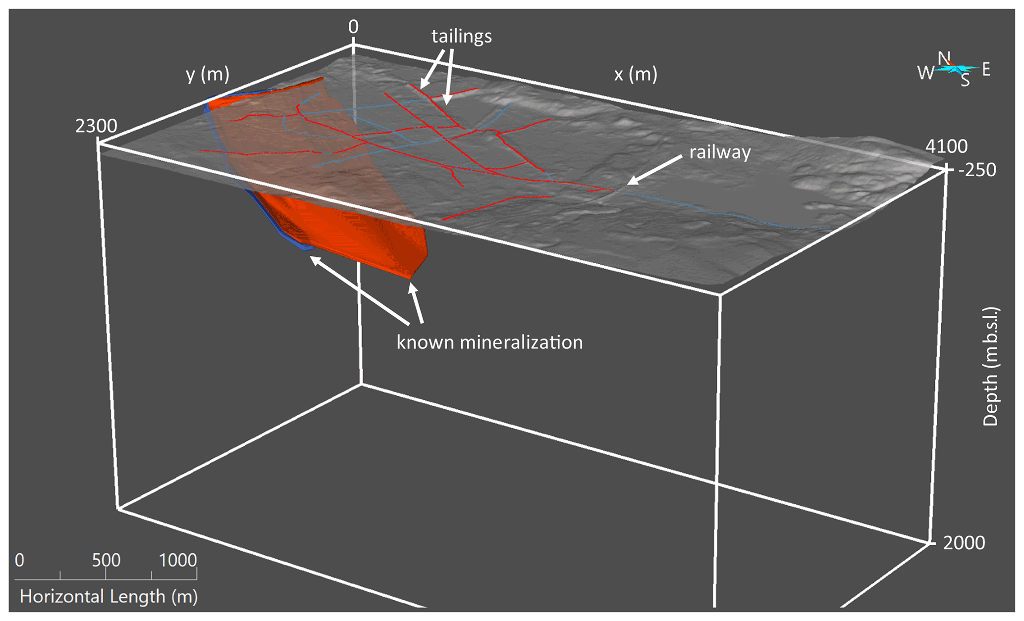
Figure 3Perspective 3D view of the known mineralization (red and blue layers and bodies) in the Blötberget area, together with the source and receiver positions (red and blue dots, respectively) of the 3D survey and a digital elevation model showing the topography in the study area.
The seismic dataset for this study was acquired during spring 2019. Figure 1 shows the geometry of the seismic survey onto the geological map, including all source and receiver locations in red and blue, respectively. The black rectangle indicates the lateral extension and location of the resulting 3D seismic cube described in detail below. Figure 3 shows a 3D perspective view of the known mineralization (red and blue surfaces; their model is based on former mining activities, borehole data, and the previously acquired 2D seismic data) and the surface topography and the acquisition geometry of the 3D survey.
The image cube (black rectangle in Fig. 1, white box in Fig. 3) has a horizontal extension of 2.3 km × 4.1 km. Its longer axis is oriented in a NW–SE direction and follows the central line of the 3D survey, which is identical to the previous 2D seismic survey acquired in 2015 and 2016. Its shorter axis runs almost parallel to the strike direction of the main geological units of interest. The vertical extension of the cube in Fig. 3 is 2.25 km (from −250 to 2000 m b.s.l.).
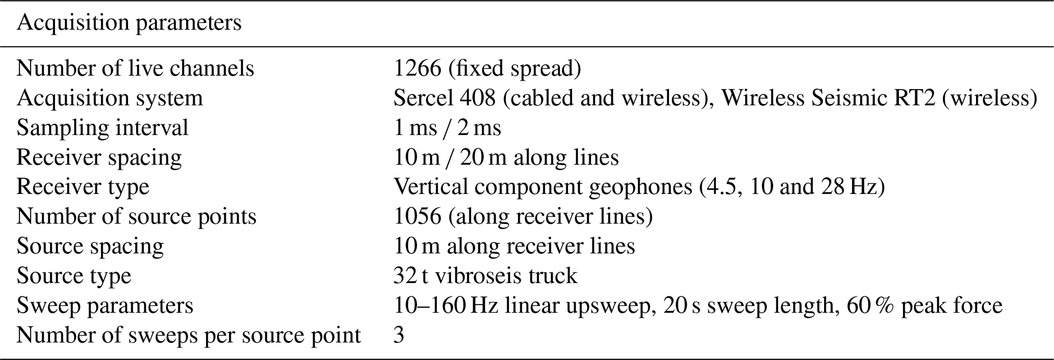
For the 3D survey a combination of cabled and wireless receivers was used with 1266 receiver points in total. The 32 t vibroseis source of TU Bergakademie Freiberg was used as seismic source with a linear up-sweep length of 20 s, a frequency bandwidth of 10–160 Hz, and vertical stacking of three sweeps per source point. Overall, 1056 source points were acquired, distributed mainly along existing forest roads in the area, resulting in a rather irregular and sparse 3D geometry. The internal receiver spacing along the lines was 10 m along three NE–SE-oriented lines and 20 m for all other lines. The northwestern part of the investigation area is covered relatively well with source–receiver azimuths in all directions, while the southeastern part contains only receiver points and no shot points along the central line. The layout was chosen like that since the mineral-deposit-related structures of interest strike from southwest to northeast and dip to the southeast. As a consequence of this survey layout, the near-surface part is covered and illuminated well in 3D (see Fig. 5 in Mahlemir et al., 2021), while the deeper central parts are presumably less well covered and illuminated. The layout of the survey was caused by two restrictions related to environmental and logistical issues. The first was the restriction imposed by the vibroseis truck on the available roads, which was a problem in the southeastern part of the central line where the truck could not enter due to weight limits on the access roads. The second limitation was related to the usage of cabled receivers and limited wireless recorders available for the survey. Moreover, the majority of the used wireless receiver system required a communication between single receivers in the field so that a linear setup was also necessary for these receivers. A minor number (10 %) of receivers were fully autonomous recording wireless stations, and these receivers were used to cross the main road interrupting the profile in the southwestern part of the layout and were distributed along the existing road that extends the layout to the southeast. All acquisition parameters are summarized in Table 1.
Table 1Acquisition parameters of the 3D reflection seismic survey.
The imaging workflow consists of three steps, which are described in detail in the following sections. The first step is the signal pre-processing of the data in the time domain. This step includes static corrections, which are handled later. The second important part in our imaging workflow is the creation of a macro-level velocity model that, together with the pre-processed data, serves as an input for pre-stack depth migration, which is the final step in the workflow.
4.1 Data pre-processing
Figure 4 shows an exemplary single shot gather before and after pre-processing. In general, the dataset exhibits an excellent quality with good signal-to-noise ratio for such a hard-rock setting, with sharp first arrivals and several clear reflections already visible in the raw shot gathers (Fig. 4a). The dataset has been pre-processed following the processing flow listed in Table 2. The focus in the signal-processing sequence was on a consequent suppression of surface waves and the boosting of the coherency of the reflected signals from the ore bodies and their surrounding structures. The low-frequency surface waves (orange ellipses in Fig. 4) were successfully suppressed, and the visible reflection signals are enhanced. The latter appear clearer and more continuous along the single-receiver lines and are traceable throughout the whole shot gather (see yellow arrows in Fig. 4b).
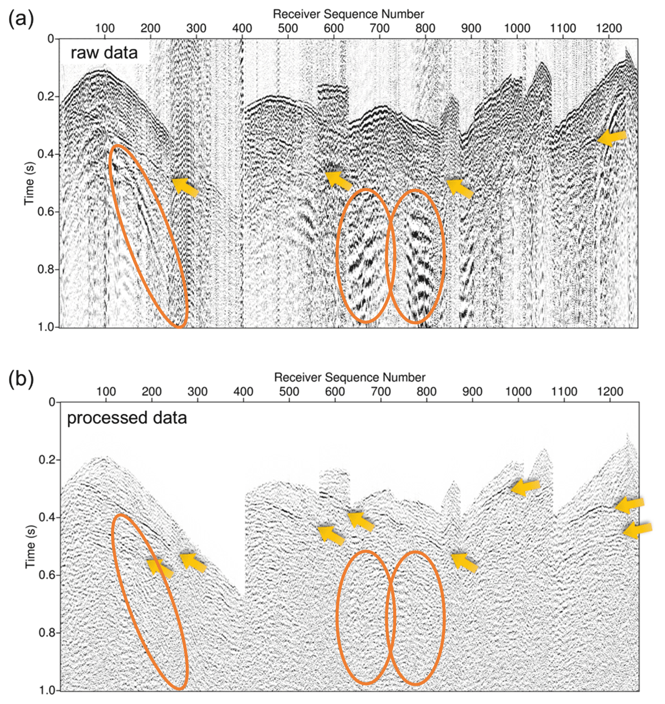
Figure 4An example shot gather of (a) the raw data and (b) the data after pre-processing as described in Table 2. The source position of the shown shot gather is located close to receiver number 1250. The yellow arrows mark some visible reflections interpreted as being caused by the mineralization in the data; the orange ellipses exemplary mark surface waves present in the raw data.
Table 2Pre-processing flow applied to the dataset. All steps up to amplitude scaling are identical up to step 5 in the processing method given in Table 2 of Malehmir et al. (2021).

4.2 Refraction statics
In order to adequately account for the influence of the near-surface low-velocity weathering layer in combination with widely varying topography, we use 3D refraction static solutions based on a 3D first-arrival travel time inversion, followed by a shift to the final datum using a constant replacement velocity, which is in the range of the expected surface bedrock velocity in our investigation area. Static corrections are reasonable in some cases as they basically remove the influence of the complete near-surface weathering layer from the data. Since the velocities below the weathering layer are expected to be slowly varying both laterally and with depth, a simple macro velocity model can then be used in the next step for migration.
The first arrivals were manually picked for the whole dataset and used to calculate refraction statics using two methods available in the used processing software (TomoPlus from Geotomo Inc.): (1) generalized refraction travel time inversion (GLI3D, Hampson and Russell, 1984) and (2) first-arrival travel time tomography (FATT) (Zhang and Toksöz, 1998). GLI3D is a very robust technique to invert refraction travel times using a layer-based model. Velocities in layers can vary laterally, except the shallowest one. Nevertheless, the thickness is allowed to vary also for this, mostly thin, layer and thus resolve the near-surface layer sufficiently. FATT can be used to derive static solution in form of so-called tomostatics (e.g., Bräunig et al., 2019). This method can be advantageous over layer-based inversion in the case of strong topography or a lack of clearly defined refraction interfaces, e.g., in mountainous areas (Cyz and Malinowski, 2013). On the other hand, there is an ambiguity in determination of the intermediate datum in tomostatics, which can affect final statics values. In the case of the hard-rock seismic setting, a simple two-layer refraction solution is usually used to represent glacial sediments and the bedrock.
We tested both methods for the Ludvika data, using all the available picks in the inversion. The GLI3D solution was based on a two-layer model. For the residual static calculations, only offsets between 200 and 2000 m were used. Looking at the common-receiver and common-shot stacks without a statics application (Fig. 5a and d), it is clear that statics are a significant issue in our data. Although the receiver and shot static values obtained using both methods do not differ significantly, one can see that there is a better alignment of the energy visible in the stacks produced with the application of the GLI3D statics (Fig. 5c and f) compared to the alignment in the stacks of tomostatics (Fig. 5b and e), especially for the shot stack (e.g., in the vicinity of shot 800; see arrows in Fig. 5). Therefore, our final choice was to apply the GLI3D-derived statics to the data. This choice allowed us to avoid a potential problem related to the fact that application of the residual part of the statics to the data would be required in order to properly use tomostatics in the depth-imaging workflow. Furthermore, we would need to set the migration travel time calculation grid fine enough to be able to reproduce the long-wavelength part of the tomostatics. This approach would have been computationally too expensive in 3D (Jones, 2018).
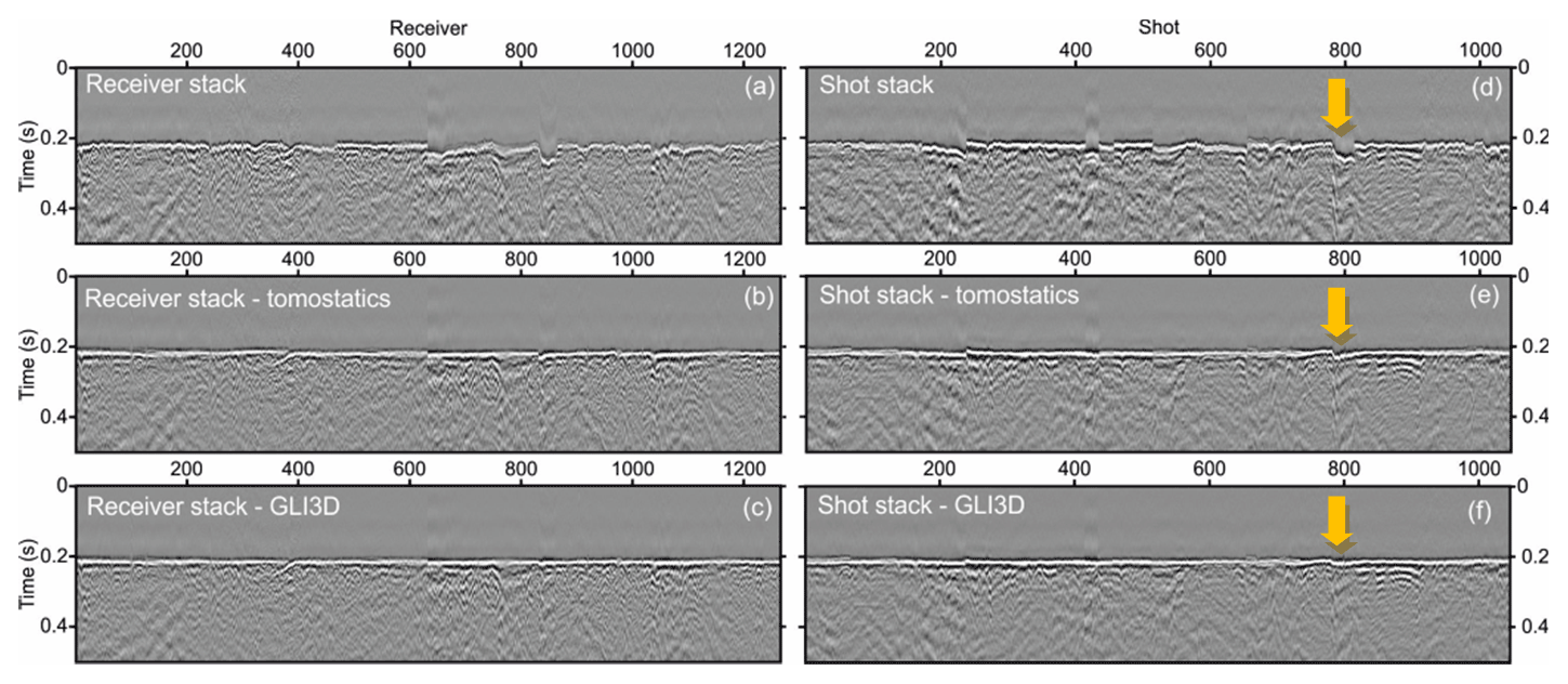
Figure 5(a–c) Common-receiver and (d–f) common-shot stacks calculated for the data after a simple linear-moveout (LMO) correction and with the application of the tomostatics (b–e) and GLI3D statics (c–f).
4.3 Migration velocity model building
As an input for pre-stack depth migration techniques, a good macro velocity model in depth is needed. However, creating such a reliable migration velocity model can be a challenging task for hard-rock settings, since clear reflections are often missing while required for picking velocities within conventional velocity semblance analysis. What is also very special in such hard-rock environments is the relatively homogeneous velocity distribution within crystalline formations, combined with relatively small velocity variations between different rock types and typically slightly increasing velocities with depth. Velocities up to 6000 m s−1 often appear already at shallow depths. In combination with an additional weathering layer in the uppermost part, which is typically characterized by low velocities (<2000 m s−1) and significant heterogeneity, a strong vertical velocity gradient can often be observed in the shallowest part of the subsurface. A high-resolution near-surface velocity model would be required to accurately address this shallow strong velocity gradient (Jones, 2018). This would lead to a densely sampled migration velocity model (and therefore a high computational effort), while the velocities in the hard rock itself vary only very smoothly.
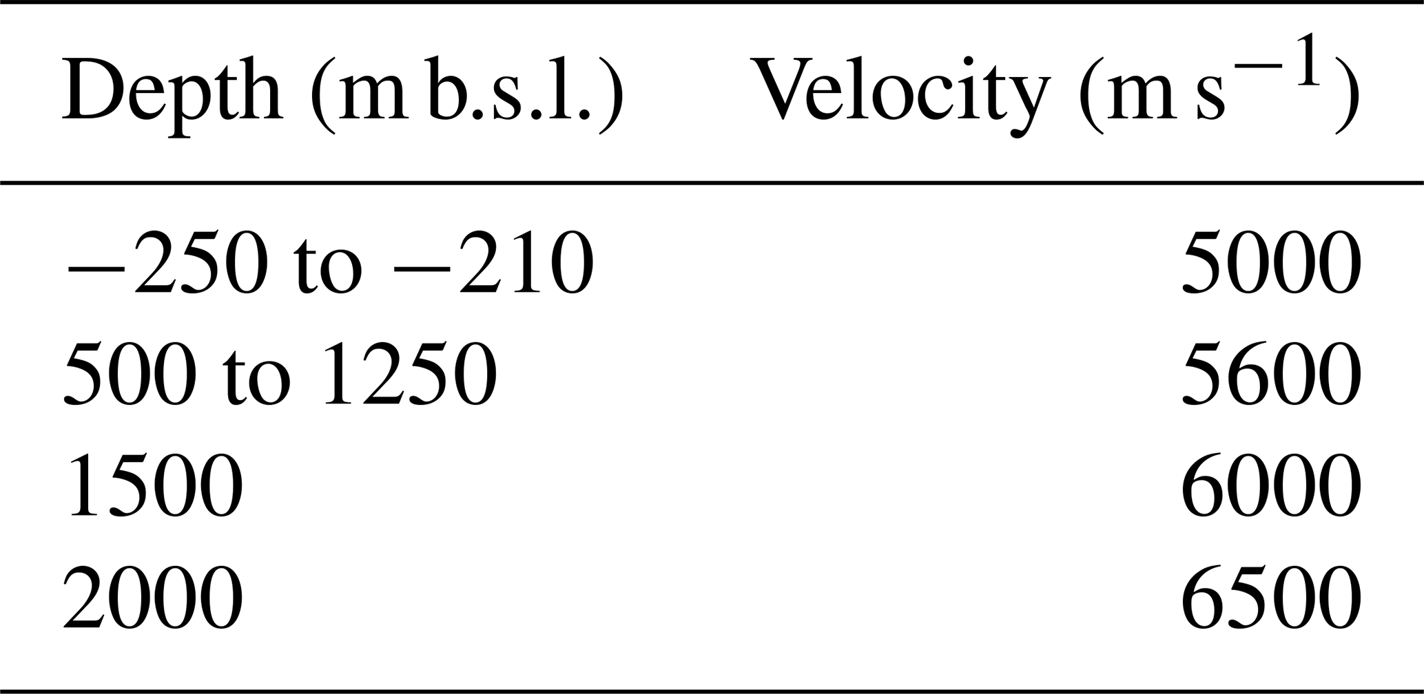
Here, the inverted near-surface velocity model was only used to calculate static corrections, in contrast to the imaging workflow described in Bräunig et al. (2019) where the near-surface velocity model was also used directly as part of the migration velocity model. Borehole investigations (Maries et al., 2017) have shown that the bedrock velocities are in the range of 5600 m s−1 down to the target depth. Bräunig et al. (2019) used a migration velocity analysis (MVA) approach to extend the migration velocity model below the shallow tomographic model down to the target depth, also including the borehole logging information from Maries et al. (2017). As a constraint, common image gathers with the mineralization-related reflector as a key horizon were used to iteratively update and improve the velocity model. Therefore, the derived velocity model can be considered to be reliable down to the depth of the expected mineralization. Here, we use the MVA-derived part of the migration velocity model, which is basically a 1D gradient velocity model with slightly increasing velocities with depth. At the top of the velocity model, we use the replacement velocity, which was also used during static corrections, as a starting value for the 1D gradient model. The velocity values and the corresponding depths are summarized in Table 3. The values are linearly interpolated between the depth intervals and are kept constant within the depth intervals.
4.4 Pre-stack depth migration
The application of the pre-stack depth migration plays a major role as the final step in our workflow. As for the 2D data, we initially applied KPSDM (Schneider, 1978; Buske, 1999), resulting in a first 3D seismic depth image of the investigation area. Subsequently, we applied FVM as an extension of KPSDM that limits the migration operator to the Fresnel volume around back-propagated rays and focuses the image on the physically contributing part of the two-way travel time isochrone (Lüth et al., 2005; Buske et al., 2009). FVM was applied successfully to prior hard-rock reflection seismic data in 2D and 3D (e.g., Hloušek et al., 2015b; Riedel et al., 2015; Hloušek and Buske, 2016; Jusri et al., 2018; Bräunig et al., 2019), including mineral exploration (Heinonen et al., 2019; Singh et al., 2019). A key point in 3D FVM is the 3D slowness estimation from the recorded data. The slowness is estimated directly from the recorded wavefield using a local slant stack method with the semblance (Neidell and Taner, 1971) as a measurement of wavefield coherency. It can handle arbitrarily distributed receivers to estimate the most probable direction for the emergent wavefield (Hloušek and Buske, 2016). Hence, the slowness estimation (and therefore FVM) is completely data driven and needs no a priori information on strike and dip directions of the expected structures. This ability to image arbitrary dips and strikes without a priori information makes FVM extremely robust for imaging in hard-rock environments, especially when the signal-to-noise ratio is low, the coverage of the data is sparse and the impedance contrasts of the expected structures are small, as shown in Heinonen et al. (2019). Therefore, we used FVM as the preferred imaging technique for the 3D dataset here in this study.
The pre-stack depth migrations (KPSDM, FVM) were applied to each shot separately. The migration is performed on a uniform grid with a spacing of 10 m in each direction. The result is a 3D image for each shot gather, and these are finally stacked to form the complete image (Buske, 1999).
As a first step, a constant migration velocity of 5600 m s−1 as a representative value for the bedrock in the investigation area was chosen for KPSDM in order to get an overview about the main structures and an impression of the reliability and robustness of the applied pre-stack depth-migrated approach. Figure 6a and b show vertical depth slices of the resulting image cube along the northeast–southwest direction through the central part of the investigation area. Figure 6a shows the plain image with two marked reflectors. The yellow arrows mark the expected main mineralization reflector, which is dipping to the southeast. At its lower end, this reflector is bounded by a crosscutting reflector (blue arrows), which is dipping into the opposite direction. This crosscutting reflector was also present in the result of the earlier 2D survey (Bräunig et al., 2019; Markovic et al., 2020), but here this reflector appears much clearer and sharper. Several other reflectors can already be found in this 3D KPSDM image, which will be described in detail using the FVM image below. Here, we concentrate on the two mentioned reflectors for the evaluation of the imaging techniques and the used velocity model. The dip direction and dip angle are well visible in the seismic image. However, a detailed comparison of the image and the modeled mineralization (Fig. 6e) shows that the reflector is imaged around 50 m below the known model layers. The reason for this mismatch is due to the constant velocity of 5600 m s−1 used for the migration, which appears to be too high. Choosing iteratively different constant velocities for migration to find a representative effective medium velocity could improve the tie between the depths of the imaged reflector and the corresponding mineralization. Such an approach would be comparable using different constant velocities for a time-to-depth conversion for time domain imaging techniques. However, such a calculation of an average medium velocity will not necessarily result in a robust migration velocity model for all depths and would thus not be the best choice to improve depth positioning and the image quality along all reflectors throughout the whole 3D model. Therefore, we omit this iterative improvement and instead concentrate on a more reliable 3D migration velocity model in the next step. Before using this, we wanted to improve the seismic image and therefore applied the focusing 3D FVM approach using the constant migration velocity of 5600 m s−1. Figure 6c, d, and f show the same vertical depth slices as in Fig. 6a, b, and e but here for the FVM image cube. The arrows mark the same reflectors as in the KPSDM image: yellow arrows for the main mineralization and blue arrows for the crosscutting reflector. When comparing the KPSDM and FVM images (Fig. 6a and c, respectively) many similarities but also several significant differences can be observed. Since the used migration velocity model and the basic imaging technique are identical, the imaged structures appear at the same position and depth. Furthermore, all observable structures in the FVM image are already part of the KPSDM image, but they are partly covered by incoherent noise and migration artifacts in the KPSDM image. In general, the FVM image appears much clearer than the KPSDM image. This is caused by the restriction to the Fresnel zone along the corresponding travel time isochrones during FVM. In addition, incoherent noise is reduced in the whole FVM image and the coherent reflectors are more outstanding.
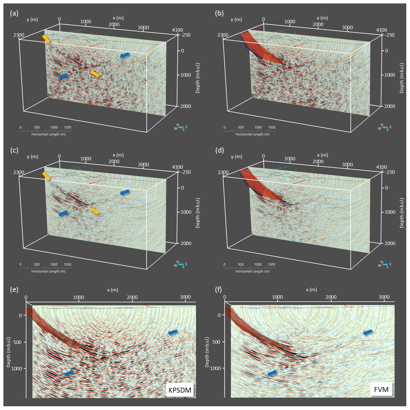
Figure 6Depth slices through the KPSDM result(a, b, and e) and the FVM result (c, d, and f) using a constant velocity of 5600 m s−1 for migration, shown in (a) and (c) without and in (b) and (d) with the known mineralization layers in red and blue. The yellow and blue arrows in (a) and (c) mark the image of the main mineralization reflector and a crosscutting reflector dipping in the opposite direction. Panels (e) and (f) are a 2D view of the results for KPSDM and FVM, respectively. The gain for plotting was chosen such that the reflectors of the main mineralization appear in the same intensity for both techniques (KPSDM and FVM).
To evaluate the quality of both migration results, we try to estimate the signal-to-noise ratio for both image cubes from KPSDM and FVM. Therefore, we normalize both volumes to the root mean square (rms) of all amplitudes in the volume so that the variability of the amplitudes is in the same range. In a second step we calculate the median amplitude for all images and set this median in relation to the rms value, assuming that the median amplitude value is representative for the noise present in the image cube. The ratio of these two values can be seen as improved signal-to-noise ratio and yields a roughly 7 times higher signal-to-noise ratio of the FVM image in comparison to the KPSDM image. Due to the improved signal-to-noise ratio, the crosscutting reflector appears more continuous. Its shallow part in the southeast is especially visible in the FVM image (upper blue arrow in Fig. 6c), while it is covered by incoherent noise in the KPSDM image (Fig. 6a). Overall, the imaged reflectors are more continuous and easier to identify in the FVM result.

Figure 7The same depth slices as in Fig. 6 shown through the FVM result using the 1D migration velocity model and including information from MVA (Table 1) presented (a) without and (b) with the known mineralization in red and blue. The arrows in (a) mark the image of the main mineralization reflector and a crosscutting reflector dipping in the opposite direction (compare Fig. 6c and d). Panel (c) shows a frontal view of the important portion of (b) together with the main mineralization in red.
As the next step, the constant migration velocity model was replaced by the 1D gradient model described in Table 3. Figure 7 shows the FVM result using this 1D gradient model for slowness calculation, ray-tracing within FVM, and travel time calculation. The shown slice is located at the same position as the slices for the KPSDM image and the FVM image using a constant migration velocity (Fig. 6). Here, the same main structures can be identified. The reflector related to the main mineralization is marked again with yellow arrows. Compared to the previous results it is imaged slightly shallower but with approximately the same dip angle. The reflector itself is more coherent than in the case of a constant migration velocity (Fig. 6) and the image of the reflector appears straighter in its shape. The crosscutting reflector, marked with blue arrows in Fig. 7a and c, is also imaged at shallower depths. In contrast to the main mineralization, the dip of the crosscutting reflector appears steeper when using the 1D gradient velocity model instead of the constant velocity for migration. Furthermore, the image of the reflector is more coherent and exhibits a higher amplitude. Figure 7b and c shows the FVM image based on the 1D gradient together with the known mineralization (blue and red bodies). The image of the reflector coincides precisely with the depth position and dip of the known mineralization. At the lower end of the model, the imaged reflector continues down to greater depth and further to the southeast, where it ends at the crosscutting reflector.
Figure 8 shows a selection of other vertical depth slices through the FVM image cube based on the result using the 1D gradient velocity model. The slices are all oriented from northwest to southeast and have a spacing of 100–200 m. The location of each slice in the local coordinate system is indicated in the upper right corner of each subfigure. The slice in Fig. 8a, located in the northeast of the investigation area, shows a prominent reflector marked with M1, and this reflector can directly be correlated to the upper main mineralization (red layer in Fig. 3). In this slice, the image of the reflector appears relatively curved and interrupted in the middle part. The curvature can be explained by the image being affected by migration artifacts (migration smiles) due to the fact that the slice is located at the boundary of the investigation area and therefore being insufficiently illuminated. This could also be the reason for the interruption in the middle part of the reflector. Below the main reflector M1, several other low-amplitude reflectors can be identified. In the second slice (Fig. 8b), the reflectors are better illuminated. Now, the reflector M1 appears as a high-amplitude coherent reflector with only a slight curvature at the upper northwestern end. It dips about 30∘ to the southeast and is imaged between 240 and 840 m depth. The dip angle and dip direction are in good agreement with the dip of 25 to 30∘ in the time-migrated and depth-converted image of Malehmir et al. (2021). The reflectivity below the M1 reflector in Fig. 8b appears more coherent than in Fig. 8a and distinct reflectors can be identified (green arrow). Furthermore, the previously described crosscutting reflector (compare with Fig. 7) is well visible (C1, blue arrow in Fig. 8b). It dips with an angle of approximately 25∘ to the northwest and is imaged between 400 and 740 m depth. The reflectors M1 and C1 are intersecting at 725 m depth, where the C1 reflector marks the lower end of the coherent and straight image of the M1 reflector.
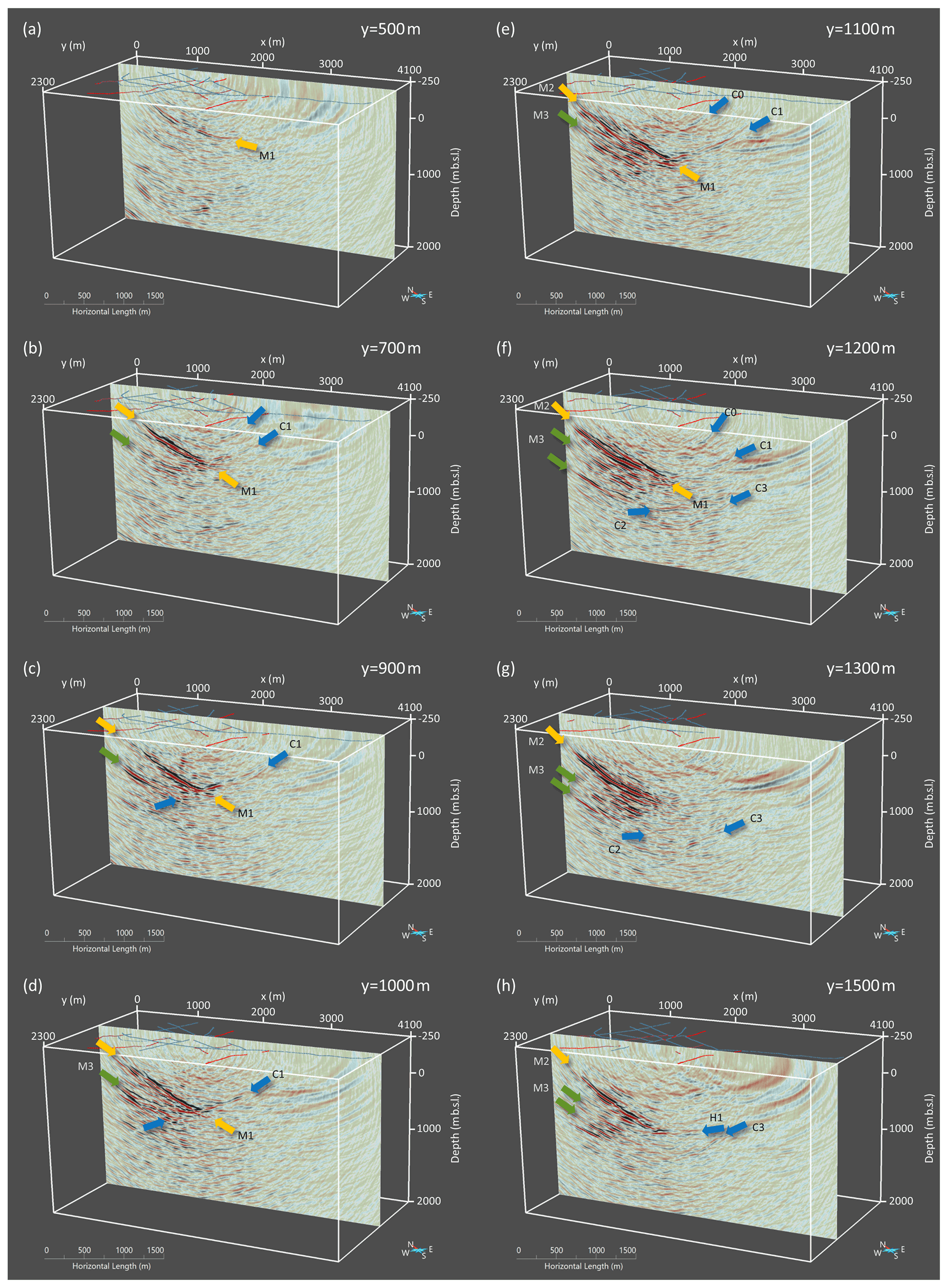
Figure 8Depth slices through the final FVM result based on the 1D migration velocity model. The sections in (a) to (h) are spaced by 100–200 m in the y direction. Several reflectors are named and marked with arrows: yellow marked reflectors correspond to the known mineralization, reflectors marked with green arrows are located subparallel below the known mineralization, and blue arrows indicate reflectors dipping into the opposite direction of the known mineralization.
Beside the C1 reflector, a second weaker reflector is visible at shallower depth (blue arrow). It dips about 20∘ to the southeast and is imaged between 160 and 360 m depth. This reflector is traceable only over some slices. In Fig. 8c, it is almost not visible anymore. The M1 reflector appears again as a sharp and strong reflector. The dip is still around 30∘, but the reflector can be traced between 35 and 830 m depth with a spatial extent of approximately 1700 m in this slice. It is again crossed at its lower end at 780 m depth by the C1 reflector. The latter is imaged slightly deeper than in the previous slice and shows approximately the same dip angle of about 25∘. This changing depth suggests a 3D orientation of this reflector, which is not perpendicular to the slices selected here. Since the imaged depth is increasing, the true strike direction is oriented north–south. However, it is imaged clearly between 250 and 990 m depth. Above the intersection with M1, it is imaged as one continuous reflector, while it appears more disrupted below the intersection, where it also intersects other coherent reflectors that are oriented subparallel to the M1 reflector (green arrow). This reflector is imaged between 500 and 1000 m depth and is dipping with almost the same angle as reflector M1 to the southeast. The lower end of this reflector is also marked by the crosscutting C1 reflector. Besides these main reflectors, some deeper and less strong and coherent reflectors can also be observed. They are all dipping to the southeast and with an angle around 30∘, comparable to the M1 reflector.
In the following slice Fig. 8d, the overall structures are imaged in a similar pattern. The depth of the C1 reflector is slightly increasing, the reflector appears less continuous than before and shows a small offset at 480 m depth. The M1 reflector also appears less continuous, and it is less sharp and coherent, especially in the upper part. The deeper subparallel reflector also appears less coherent and continuous together with a broadened signature, which also accounts for a more complex 3D structure for the M1 reflector and the underlying reflectivity. This impression is confirmed by the image in the next slice at y=1100 m (Fig. 8e). There, the reflector M1 can still be identified but is also intersected by a second, slightly deeper reflector with the same dip direction (M2). In addition, the underlying subparallel reflectivity appears even more complex and less distinct than before. All reflectors dipping to the southeast are confined by the crosscutting C1 reflector at their lower end. The image again becomes clearer in the next slice (Fig. 8f), where the M2 reflector becomes the most prominent and coherent reflector. It is imaged between 190 and 770 m depth and dips with an angle of about 30∘ (the same dip as M1 reflector) to the southeast. The M1 reflector can be identified only in deeper parts between 550 and 780 m depth with a slightly steeper angle than the M2 reflector. Below these two reflectors, some parallel reflectors are again visible with approximately the same dip direction (marked with two green arrows). The C1 reflector is still visible, although the signal is weaker compared to the previous slices. Here, several other reflectors with a comparable dip direction are present and marked with C0, C2, and C3. These reflectors exhibit a shorter spatial extent compared to the others and are traceable only over some adjacent slices. Reflectors C2 and C3 can also be found in the next slice (Fig. 8g). They appear approximately at the same location, whereas the C1 reflector is not visible anymore. The same applies for the M1 reflector which is no longer distinguishable from the M2 reflector. The latter is imaged between 180 and 880 m depth; the underlying parallel reflectors (green arrows) are still visible but are less distinct than before. The imaged reflector in this area is more diffuse. Although reflector C1 is not directly visible, the reflectivity of the M2 reflector and the underlying reflectors end along a line that has the same dip as the C1 reflector before. The reflectivity in the last slice (Fig. 8h) is again more coherent. The M2 reflector is imaged sharper and is also steeper (35∘) than in Fig. 8b to g. The lower end is confined by an almost horizontal reflector (H1). The reflector C3 is still visible and shows a slightly listric shape. The underlying reflectivity (green arrows) is still present in this image.
The visibility of the important structures in the seismic volume can be summarized as follows: the M1 and M2 reflectors can be traced over all shown slices. Since they are crossing each other and intersecting in some slices, it is not always possible to distinguish between both reflectors. In all shown slices, an underlying reflectivity can be observed. It consists of partly distinct reflectors that are dipping in the same direction and with a comparable dip angle to that of the reflectors M1 and M2. The lower end of this reflectivity and the reflectors M1 and M2 is confined by the crossing C1 reflector, which has an apparent dip in the opposite direction. Since the imaged depth is increasing for slices to the southwest, the strike direction of this reflector appears more towards the north–south rather than the northeast–southwest direction. This orientation also explains why this reflector vanishes in the slices in the southwest because it is presumably not illuminated by the combination of sources and receivers anymore. However, the reflectivity of the M1 and M2 reflectors, as well as the reflectivity of the underlying reflectors, still ends at a line, which could be an indirect hint toward a lateral continuation of the C1 structure. A more detailed geological interpretation in relation to the known structures is given in the following section.
The main mineralization, including its surrounding host rock structures like the major crosscutting fault, are successfully imaged, which is the basis for further structural interpretation. The reflectors related to the mineralization are clear, pronounced, and with high amplitudes. They are partly intersecting with varying characteristics in lateral direction, and in some parts they exhibit a rather complex 3D shape. In order to constrain the validity of the image, a detailed comparison of the imaged structures with the geological model of the known mineralization assessed in a detailed view on the FVM image, together with the current model of the second known mineralization (Fig. 9, blue body, M2). The imaged position, the dip, and the general shape of the reflectors fit almost perfectly to the corresponding position of the known geological model of the ore bodies. Furthermore, the reflector corresponding to the main mineralization (blue body in Fig. 9) is traceable at least 300 m further downward from the known downdip end of the mineralization. Additionally, the seismic image reveals a bowl-type shape (likely a tight fold) of this reflector in crossline direction (parallel to the main strike direction), which can be followed laterally even further upward beyond the known model of the mineralization (yellow ellipse in Fig. 9a).
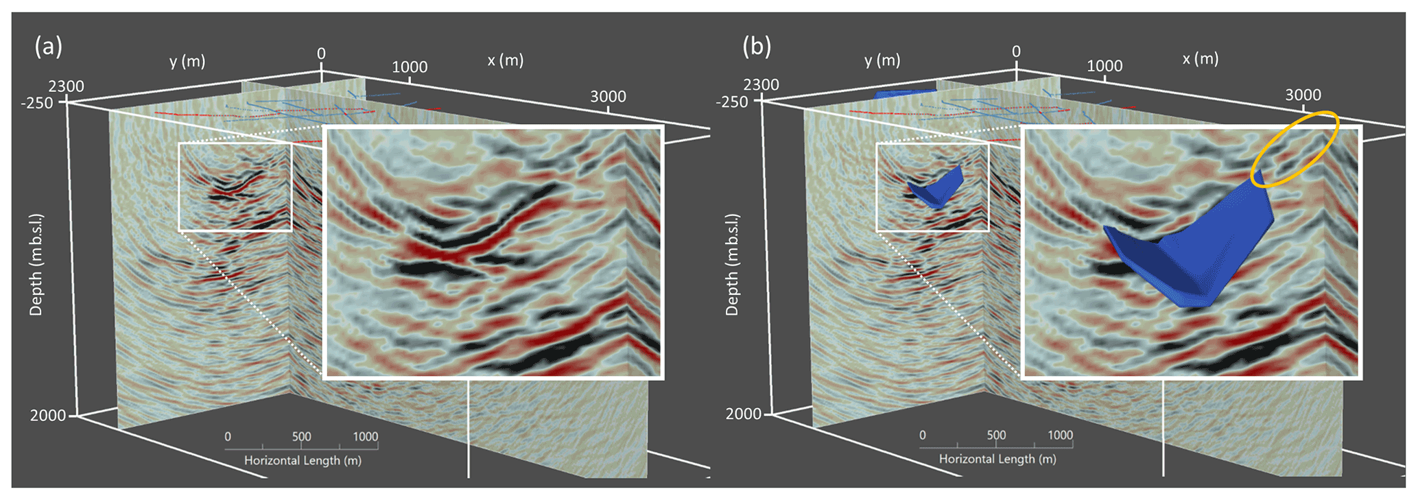
Figure 9Perspective view (a) without and (b) with the model of the known mineralization (blue body). The zoomed inset shows the good agreement of the position, depth, and shape of the known mineralization and the corresponding reflectors in the seismic image.
We tried to trace all imaged reflectors in the 3D FVM image cube and manually picked the horizons to verify, complement, and extend the known structural model of the mineralization and its host rock structures. The reflectors were picked only when they showed coherent and strong amplitude over a certain distance and were clearly traceable within the 3D seismic image cube. Indirect structural indicators like phase offsets along the reflectors or positions where reflectors seemed to be truncated were not picked. Furthermore, partly reflective structures were not automatically connected, but they were instead left as separate surfaces so that the interpretation of their possible connection was left as objective as possible. The picked horizons are shown in Fig. 10. Figure 10a and b represent perspective views on the models of the known mineralization together with the picked horizons. The view direction is from south to north (Fig. 10a) and from east to west (Fig. 10b), respectively. The picked horizons M1 and M2 are shown in red and blue in accordance to the known mineralization bodies, and the crosscutting reflector C1 is shown in gold. For the picked C1 reflector, the corresponding horizon extends downward to its lower end at a depth of approximately 1000 m. It is illuminated by the source–receiver geometry mainly in the central part of the investigation area. It presumably continues further up the dip (to the southwest), but with the given acquisition geometry it is not possible to illuminate it further towards the surface. The same applies to the lower end of this reflector. It is possible that the structure may continue deeper, but it is not illuminated by the acquisition geometry. However, an extrapolation of this horizon (in form of a mean plane for all picks, purple plane in Fig. 10c) shows its possible continuation within the image cube. The surface outcrop of this extrapolated horizon would be located in the western part of the image cube with an almost north–south strike direction. Figure 10d shows where the mean plane would reach the surface and its relation to the known mapped surface geology. The surface location and strike direction of the mean plane fits perfectly to a mapped lineament in the geological map (yellow arrows in Fig. 10d). Therefore, it is highly likely that this mapped fault and the imaged reflector refer to the same structure.

Figure 10Interpretation of the identified and picked horizons. Panels (a) and (b) show perspective views on the picked horizons and the model of the known mineralization. The crosscutting reflector C1 is extrapolated using a mean plane (purple plane c), which intersects with the surface at a mapped fault line (yellow arrows in d). The view in (d) is identical to (c) but includes a map of the surface geology (courtesy of the Geological Survey of Sweden).
As described above, the two main reflectors M1 and M2 show the same location, dip angle, and shape as the known mineralization. In addition to this agreement, the reflectors show an about 300 m lateral and downward continuation of the previously known mineralization, meaning a potential continuation of the mineralized bodies and therefore additional resources. Assuming that the crossing reflector C1 is marking the lower end of the mineralization bodies would allow us to fill the gap between C1 and M2, which means an even larger downward continuation for this reflector, which is directly visible in the FVM image.
Some of the reflectors can be directly related to the geology. M1 and M2 can clearly be interpreted as reflected signals from the boundary between the host rock and the main mineralization, which is known to be characterized by a relatively high impedance contrast. Both reflectors show a bowl shape of the mineralization bodies, and they are partly intersecting each other. The imaged reflectors also indicate a potential greater lateral extension of the mineralization.
The underlaying reflectivity (green arrows, M3) is only partly coherent and shows a shorter lateral extension, but as the strike and dip directions are identical to the overlaying mineralization, we interpret these reflectors as also being mineralization related, meaning that there are potential additional resources for this deposit.
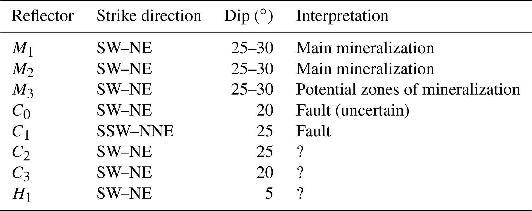
Since C1 can be linked to a surface trace of a fault, it can be interpreted as such. The weaker and shorter C0 reflector can also be interpreted as a fault or as the contact zone between intrusive and volcanic rocks (see also Fig. 1). The other imaged reflectors (C2, C3 and H1) are imaged only at greater depth, and thus no direct link to the surface geology is possible. A remarkable fact for these reflectors is that they are imaged in the vicinity of the lower end of the imaged mineralization. They could be related to the formation of the whole deposit.
Table 4Characteristics and interpretation of the imaged reflectors.
A comparison to the post-stack time-migrated and time-to-depth-converted result by Malehmir et al. (2021) shows many similarities but also some differences. The main imaged reflectors (M1, M2 and C1, or F1 in Malehmir et al., 2021) are present in both results. The C1 reflector is much better imaged in the pre-stack depth image from FVM. Here it appears as a relatively sharp and continuous reflector, especially in the direct vicinity of the lower end of the M1 and M2 reflectors. In contrast, the post-stack time migration image of this reflector is only piece-wise evident and less continuous, but it is also imaged in shallower depths. The reason for the better image here is presumably the opposite dip of the intersecting reflectors (C1 and M1, M2), which have to be adequately addressed during stacking in the post-stack approach and might have caused some problems. In contrast, the different dip directions are naturally handled by the pre-stack depth-migration approach, and as such the reflectors are imaged properly. Furthermore, the sharp image of the FVM allows for a detailed interpretation of the visible reflectivity and for tracing individual reflectors through the migrated volume. Thus, we were able to map the M1 and M2 reflectors, resulting in the fold shape seen in Fig. 9. Finally, the application of pre-stack depth-migration directly results in a depth image rather than a time image. For the latter, a post-migration, time-to-depth conversion is needed in order to interpret the seismic image in depth. This conversion is done often with a velocity or a velocity–depth function to best fit a priori (e.g., borehole) information. The pre-stack depth image shown here is completely data driven and nevertheless fits well with the a priori information. This means that a high reliability of the resulting seismic image and especially the imaged depths and dips of the visible reflectors can be assumed. The used imaging techniques, in conjunction with a careful pre-processing of the data, are applicable and well tailored for mineral exploration in hard-rock environments. Any a priori information can be used for further optimization and validation. In that sense, such imaging approaches are also interesting for the exploration of less well-known or explored potential mineral deposits.
Potential avenues for future work include the incorporation of a more detailed P-wave velocity model derived from, e.g., full waveform inversion (Singh et al., 2021) for static corrections or even directly as part of a 3D migration velocity model. Furthermore, the acquired 3D dataset could be used for a 3D MVA using focusing pre-stack depth migration techniques to generate common offset images, which then can be sorted into common image gathers depending on not only the offset but also the angles of illumination. Since the imaged structures are characterized by different strike directions and inclination angles, together with conflicting dip situations, more advanced investigations could be helpful. The already performed slowness calculation, which is needed for back-propagating the rays within FVM, could be used to distinguish between different emergent angles and directions for the reflected signals within the application of focusing 3D pre-stack depth migration variants. In order to improve the reliability of the imaged structures and their shape, a proper illumination study should be considered. This would also help to decide if the imaged reflectors ending at depth are really ending where they appear to or if they are simply not illuminated.
Furthermore, the obtained structures are currently analyzed and interpreted together with other geophysical findings and geological data in order to obtain a comprehensive 3D model of the mineral deposit. The latter can then serve as a reliable basis for prospective modeling and estimates of its economic potential.
The acquired sparse 3D dataset provides an excellent basis for the application of seismic processing and imaging techniques in the framework of mineral exploration in hard-rock geological settings. Our workflow includes the application of a tailored pre-processing flow, as well as the application of a 3D Fresnel volume migration depth-imaging technique. Both steps are accompanied by 3D first-break travel time inversion to obtain static corrections within the processing flow, instead of handling static shifts through the detailed velocity model incorporated in travel time calculation, which would not be practical, as it requires very fine model discretization. The application of static corrections allows for the use of a simple 1D gradient velocity for the migration. It results in a sharp image of the subsurface structures with a rather high accuracy in depth positioning and allows for a detailed interpretation. Nevertheless, all reflectors were also imaged using a constant migration velocity model, but they appear with a less accurate dip and depth in the 3D volume.
The chosen processing approach delivered a high-quality 3D seismic cube with several distinct structural features that could be correlated to the known mineralization and also provide information of its possible extension in lateral direction as well as towards greater depths. The study has shown that reflection seismic methods and depth-imaging algorithms can also deliver a high-resolution 3D seismic image for sparse and irregular acquisition geometry.
The presented data are available by contacting project coordinator Alireza Malehmir or the corresponding author.
AM and PM designed the survey. AM, MaM, LB, SB, LS, EB, and FH contributed to the data acquisition. MiM performed the signal processing and calculated the static corrections. FH wrote the main content of the manuscript, applied KPSDM and FVM, and created the 3D interpretation of the seismic data. All authors contributed to the interpretation and discussion of the results and to discussions during the processing of the data.
At least one of the (co-)authors is a member of the editorial board of Solid Earth. The peer-review process was guided by an independent editor, and the authors also have no other competing interests to declare.
Publisher’s note: Copernicus Publications remains neutral with regard to jurisdictional claims in published maps and institutional affiliations.
This article is part of the special issue “State of the art in mineral exploration”. It is a result of the EGU General Assembly 2020, 3–8 May 2020.
We thank all colleagues, students and young professionals involved in the project Smart Exploration. A special thanks to all people involved in the fieldwork of the 2019 survey and NIO for their support for planning and during the field campaign. The GOCAD Consortium and Paradigm are thanked for providing an academic license for GOCAD for 3D visualization and interpretation of the data. We acknowledge the usage of the vibroseis truck of the Technische Universität (TU) Bergakademie Freiberg, operated by the Institute of Geophysics and Geoinformatics and funded by the Deutsche Forschungsgemeinschaft (DFG) under grant no. INST 267/127-1 FUGG, which was used as the seismic source in this survey. We also gratefully acknowledge the Halliburton Software Grant to the Technical University Bergakademie Freiberg, which enabled part of the data processing with their software package SeisSpace/ProMAX. The depth migrations were calculated with the help of the HPC cluster at TU Bergakademie Freiberg (DFG-grant INST 267/159–1 FUGG). Th Institute of Geophysics, Polish Academy of Sciences, acknowledges the use of the Globe Claritas seismic processing package under the academic license from Petrosys Ltd and the TomoPlus software (Geotomo Inc.). We thank Juan Alcalde, Isabelle Lecomte, two anonymous reviewers, and the editors Liam Bullock and Susanne Buiter for their helpful comments and suggestions on the original and revised version of this article.
This research has been supported by the Horizon 2020 Research and Innovation Programme (Smart Exploration, grant no. 775971).
This paper was edited by Susanne Buiter and reviewed by Juan Alcalde and three anonymous referees.
Allen, R. L., Lundström, I., Ripa, M., Simeonov, A., and Christofferson, H.: Facies analysis of a 1.9 Ga, continental margin, back arc felsic caldera province with diverse Zn-Pb-Ag-(Cu-Au) sulphide and Fe oxide deposits, Berslagen region, Sweden, Econ. Geol., 91, 979–1008, 1996.
Bellefleur, G., Schetselaar, E., White, D., Miah, K., and Dueck, P.: 3D seismic imaging of the Lalor volcanogenic massive sulphide deposit, Manitoba, Canada, Geophys. Prospect., 63, 813–832, https://doi.org/10.1111/1365-2478.12236, 2015.
Berverksstatistik: Statistics of the Swedish mining in-dustry 2013, Report of Sveriges Geologiska Undersökning, http://resource.sgu.se/produkter/pp/pp2014-2-rapport.pdf (last access: 1 December 2021), 2013 (in Swedish, partly translated in English).
Bräunig, L., Buske, S., Malehmir, A., Bäckström, E., Schön, M., and Marsden, P.: Seismic depth imaging of iron-oxide deposits and their host rocks in the Ludvika mining area of central Sweden, Geophys. Prospect., 68, 24–43, https://doi.org/10.1111/1365-2478.12836, 2019.
Buske, S.: Three-dimensional pre-stack Kirchhoff migration of deep seismic reflection data, Geophys. J. Int., 137, 243–260, 1999.
Buske, S., Gutjahr, S., and Sick, C.: Fresnel volume migration of single-component seismic data, Geophysics, 74, WCA47–WCA55, https://doi.org/10.1190/1.3223187, 2009.
Cheraghi, S., Malehmir, A., and Bellefleur, G.: 3D imaging challenges in steeply dipping mining structures: New lights on acquisition geometry and processing from the Brunswick no. 6 seismic data, Canada, Geophysics, 77, WC109–WC122, https://doi.org/10.1190/geo2011-0475.1, 2012.
Crowson, P.: The European mining industry: What future? Resour. Policy, 22, 99–105, https://doi.org/10.1016/S0301-4207(96)00025-6, 1996.
Cyz, M. C. and M. M. Malinowski: Comparison of refraction and diving wave tomography statics solution along a regional seismic profile in SE Poland, in: 75th EAGE Conference & Exhibition incorporating SPE EUROPEC 2013, London, UK, 10–13 June 2013, 348 p., European Association of Geoscientists & Engineers, https://doi.org/10.3997/2214-4609.20131102, 2013.
Dubiński, J.: Sustainable Development of Mining Mineral Resources, Journal of Sustainable Mining, 12, 1–12, https://doi.org/10.7424/jsm130102, 2013.
Eaton, D. W., Milkereit, B., and Salisbury, M. (Eds.): Hardrock seismic exploration, SEG, Tulsa, USA, ISBN: 978-1-56080-114-6, 2003a.
Eaton, D. W., Milkereit, B., and Salisbury, M. (Eds.): Seismic methods for deep mineral exploration: Mature technologies adapted to new targets, The leading edge, Society of Exploration Geophysicists, 22, 580–585, https://doi.org/10.1190/1.9781560802396, 2003b.
Hampson, D. and B. Russell: First-break interpretation using generalized linear inversion, Journal of the Canadian Society of Exploration Geophysicists, 20, 40–54, 1984.
Heinonen, S., Malinowski, M., Hloušek, F., Gislason, G., Buske, S., Koivisto, E., and Wojdyla, M.: Cost-effective seismic exploration: 2D reflection imaging at the Kylylahti massive sulfide deposit, Finland, Minerals, 9, 263, https://doi.org/10.3390/min9050263, 2019.
Hloušek, F. and Buske, S.: Fresnel Volume Migration of the ISO89-3D data set, Geophys. J. Int., 1273–1285, https://doi.org/10.1093/gji/ggw336, 2016.
Hloušek, F., Hellwig, O., and Buske, S.: Three-dimensional focused seismic imaging for geothermal exploration in crystalline rock (Schneeberg, Germany), Geophys. Prospect., 63, 999–1014, https://doi.org/10.1111/1365-2478.12239, 2015a.
Hloušek, F., Hellwig, O., and Buske, S.: Improved structural characterization of the Earth's Crust at the German Continental Deep Drilling Site (KTB) using advanced seismic imaging techniques, J. Geophys. Res.-Sol. Ea., 120, 6943–6959, https://doi.org/10.1002/2015JB012330, 2015b.
Jones, I. F.: Velocities, Imaging and Waveform Inversion: The Evolution of Characterising the Earth's Subsurface, EAGE Publications, ISBN: 1523119853, 9781523119851, 2018.
Jonsson, E., Troll, V. R., Hogdahl, K., Harris, C., Weis, F., Nilsson, K. P., and Skelton, A.: Magmatic origin of giant “Kiruna-type” apatite-iron oxide ores in central Sweden, Scientific Reports 3, 1644, https://doi.org/10.1038/srep01644, 2013.
Jusri, T., Bertani, R., and Buske, S.: Advanced three-dimensional seismic imaging of deep supercritical geothermal rocks in Southern Tuscany, Geophys. Prospect., 67, 298–316, https://doi.org/10.1111/1365-2478.12723, 2018.
L'Heureux, E., Milkereit, B., and Adam, E.: 3D seismic exploration for mineral deposits in hardrock environments, CSEG Recorder, 30, 36–39, 2005.
Lüth, S., Buske, S., Goertz, A., and Giese, R.: Fresnel-volume migration of multicomponent data, Geophysics, 70, 121–129, 2005.
Magnusson, N. H.: The origin of the iron ores in central Sweden and the history of their alterations, Sveriges geologiska undersökning, Serie C, no. 643, Avhandlingar och uppsatser, Stockholm, p. 1, https://resource.sgu.se/dokument/publikation/c/c643rapport/c643-rapport.pdf (last access: 12 May 2022), 1970.
Malehmir, A., Durrheim, R., Bellefleur, G., Urosevic, M., Juhlin, C., White, D. J., Milkereit, B., and Campbell, G: Seismic methods in mineral exploration and mine planning: A general overview of past and present case histories and a look into the future, Geophysics, 77, WC173–WC190, 2012.
Malehmir, A., Maries, G., Bäckström, E., Schön, M., and Marsden, P.: Developing cost-effective seismic mineral exploration methods using a landstreamer and a drophammer, Scientific Reports, 7, 10325, https://doi.org/10.1038/s41598-017-10451-6, 2017.
Malehmir, A., Holmes, P., Gisselø, P., Socco, L. V., Carvalho, J., Marsden, P., Verboon, A. O., and Loska, M.: Smart Exploration: Innovative ways of exploring for the raw materials in the EU, in: Proceedings 81st EAGE Conference and Exhibition 2019, London, UK, 3–6 June 2019, 1–5, https://doi.org/10.3997/2214-4609.201901668, 2019.
Malehmir, A., Gisselø, P., Socco, V., Carvalho, J., Marsden, P., Verboon, A. O., and Loska, M.: Smart Exploration inspires innovative geophysical solutions for mineral exploration in Europe, First Break, 38, 51–56, https://doi.org/10.3997/1365-2397.fb2020088, 2020.
Malehmir, A., Markovic, M., Marsden, P., Gil, A., Buske, S., Sito, L., Bäckström, E., Sadeghi, M., and Luth, S.: Sparse 3D reflection seismic survey for deep-targeting iron oxide deposits and their host rocks, Ludvika Mines, Sweden, Solid Earth, 12, 483–502, https://doi.org/10.5194/se-12-483-2021, 2021.
Maries, G., Malehmir, A., Bäckström, E., Schön, M., and Marsden, P.: Downhole physical property logging for iron-oxide exploration, rock quality, and mining: An example from central Sweden, Ore Geol. Rev., 90, 1–13, 2017.
Markovic, M., Maries, G., Malehmir, A., von Ketelholdt, J., Bäckström, E., Schön, M., and Marsden, P.: Deep reflection seismic imaging of iron-oxide deposits in the Ludvika mining area of central Sweden, Geophys. Prospect., 68, 7–23, 2020.
Milkereit, B., Eaton, D., Wu, J., Perron, G., Salisbury, M. H., Berrer, E. K., and Morrison, G.: Seismic imaging of massive sulfide deposits; Part II, Reflection seismic profiling, Econ. Geol., 91, 829–834, 1996.
Neidell, N. S. and Taner, M. T.: Semblance and other coherency measures for multichannel data, Geophsics, 36, 482–497, 1971.
Paulick, H. and Nurmi, P.: Mineral Raw Materials – Meeting the Challenges of Global Development Trends, Berg Huettenmaenn Monatsh, 163, 421–426, https://doi.org/10.1007/s00501-018-0779-8, 2018.
Pertuz, T., Malehmir, A., Bos, J., Brodic, B., Ding, Y., de Kunder, R., and Marsden, P.: Broadband seismic source data acquisition and processing to delineate iron oxide deposits in the Blötberget mine-central Sweden, Geophys. Prospect., 70, 79–94, https://doi.org/10.1111/1365-2478.13159, 2021.
Riedel, M., Dutsch, C. Alexandrakis, C., Dini, I., Ciuffi, S., and Buske, S.: Seismic depth imaging of a geothermal system in southern Tuscany, Geophys. Prospect., 63, 957–974, https://doi.org/10.1111/1365-2478.12254, 2015.
Schneider W. A.: Integral formulation for migration in two and three dimensions, Geophysics 43, 49–76, 1978.
Singh, B., Malinowski, M., Hloušek, F., Koivisto, E., Heinonen, S., Hellwig, O., Buske, S., Chamarczuk, M., and Juurela, S.: Sparse 3D seismic imaging in the Kylylahti mine area, Eastern Finland: comparison of time versus depth approach, Minerals, 9, 305, https://doi.org/10.3390/min9050305, 2019.
Singh, B., Malinowski, M., Górszczyk, A., Malehmir, A., Buske, S., Sito, Ł., and Marsden, P.: 3D high-resolution seismic imaging of the iron-oxide deposits in Ludvika (Sweden) using full-waveform inversion and reverse-time migration, Solid Earth Discuss. [preprint], https://doi.org/10.5194/se-2021-122, in review, 2021.
Stephens, M., Ripa, M., Lundström, I., Persson, L., Bergman, T., Ahl, M., Wahlgren, C.-H., Persson P.-O., and Wickström, L.: Synthesis of the bedrock geology in the Bergsla gen region, Fennoscandian Shield, south-central Sweden, edited by: Bergman, S. and Kathol, B., Geological Survey of Sweden (SGU), ISBN 978-91-7403-410-3, 2009.
Urosevic, M., Bhat, G., and Grochau, M. H.: Targeting nickel sulfide deposits from 3D seismicreflection data at Kambalda, Australia, Geophysics, 77, WC123–WC132, https://doi.org/10.1190/geo2011-0514.1, 2012.
Zhang, J. and Toksöz, M. N.: Nonlinear refraction traveltime tomography, Geophysics, 63, 1726–1737, 1998.