Gravity inversion method using L₀-norm constraint with auto-adaptive regularization and combined stopping criteria

We present a gravity inversion method that can produce compact and sharp images to assist the modeling of non-smooth geologic features. The proposed iterative inversion approach makes use of L₀-norm-stabilizing functional, hard and physical parameter inequality constraints and a depth-weighting function. The method incorporates an auto-adaptive regularization technique, which automatically determines a suitable regularization parameter and error-weighting function that helps to improve both the stability and convergence of the method. The auto-adaptive regularization and error-weighting matrix are not dependent on the known noise level. Because of that, the method yields reasonable results even if the noise level of the data is not known properly. The utilization of an effectively combined stopping rule to terminate the inversion process is another improvement that is introduced in this work. The capacity and the efficiency of the new inversion method were tested by inverting randomly chosen synthetic and measured data. The synthetic test models consist of multiple causative blocky bodies, with different geometries and density distributions that are vertically and horizontally distributed adjacent to each other. Inversion results of the synthetic data show that the developed method can recover models that adequately match the real geometry, location and densities of the synthetic causative bodies. Furthermore, the testing of the improved approach using published real gravity data confirmed the potential and practicality of the method in producing compact and sharp inverse images of the subsurface.

1 Introduction

Gravity measurements have been used in a wide range of geophysical prospecting and investigations, such as in mineral explorations, engineering and environmental problems, and archeological site investigations (Hinze et al., 2013, p. 20). In general, gravity inversion is a process that is used to determine the density, size, shape and location of complex subsurface causative bodies from an observed gravity anomaly by using different mathematical modeling techniques. Thus, inversion of gravity data constitutes an important step in the quantitative interpretation, since the reconstruction of density contrast models markedly increases the amount of information that can be extracted from the gravity data.

However, a principal difficulty with the gravity data inversion is the inherent non-uniqueness and instability that also exist in any geophysical method (Al-Chalabi, 1971; Blakely, 1996, p. 216). In other words, for the given observed gravity data, there are many equivalent density distributions that can reproduce the same field data. The standard approach used to select acceptable solutions that are geologically reasonable is to use additional information about the problem by making assumptions about the following aspects: (1) the model parameters (existing information on the subsurface structure from geological or other geophysical hindsight) and (2) the data parameters (statistical properties of the inexact data, e.g., Gaussian distribution of errors). Based on these assumptions, there are two approaches in gravity inversion. The first approach fixes the density and varies the geometry. This approach is nonlinear in nature and has been studied by many authors, for instance, Lelievre et al. (2015), Camacho et al. (2002) and Camacho et al. (2011). The second approach, which is the one used in this work, fixes the geometry and varies the density. This approach is linear in nature and has been investigated by many researchers (Li and Oldenburg, 1998; Boulanger and Chouteau, 2001).

In an effort to introduce more qualitative prior information, Last and Kubik (1983) in particular developed a method called compact gravity inversion. Their strategy utilizes the compactness stabilizer to minimize the area (in 2D) or volume (in 3D) occupied by the causative body, which is equivalent to maximizing its compactness. Barbosa and Silva (1994) generalized the compact inversion method by making use of compactness along several axes using Tikhonov's regularization. In 2006, Silva and Barbosa further developed the compact inversion method with the so-called “interactive inversion”, which estimates the location and geometry of several density anomalies. They simplified their old method (Barbosa and Silva, 1994) to improve computational performance. The generalized compact and interactive inversion strongly need a priori information to yield an accurate estimation.

The compactness stabilizer (Last and Kubik, 1983), also known as the minimum-support stabilizer (Portniaguine and Zhdanov, 1999), has been borrowed and implemented by other researchers in various geophysical inversion methods (Ajo-Franklin et al., 2007; Stocco et al., 2009; Fei et al., 2018; Feng et al., 2020; Varfinezhad et al., 2020). As was demonstrated by a number of researchers (Zhdanov and Tolstaya, 2004; Rezaie et al., 2017; Feng et al., 2020; Varfinezhad et al., 2022), this stabilizer is known to yield a compact or focused geophysical model with sharp boundaries. Apart from the inversion methods which produce focused images mentioned above, sparse geophysical inversion approaches derived from L_p-norm ($\mathrm{0}\le p\le \mathrm{1}$) stabilization have been developed by many researchers – for instance, the sparse seismic reflectivity inversion method (Li et al., 2017), direct current resistivity data inversion algorithm (Singh et al., 2018), magnetic data sparse inversion method (Li et al., 2018; Fournier et al., 2020) and sparse gravity data inversion technique (Vatankhah et al., 2017; Peng and Liu, 2021), to mention only a few.

Some instability of the original compact gravity inversion algorithm of Last and Kubik (1983) was reported by Lewi (1997, p. 87) when the data were contaminated with noise. Then Lewi (1997, p. 89) improved the original compact inversion by introducing a new approach to the 3D compact gravity inversion. The problem with the method of Lewi (1997, p. 89) arises when dealing with a multiple-source model, where the inversion algorithm tends to concentrate densities towards the surface regardless of the true depth of the causative bodies. In overcoming this drawback, Gebre and Lewi (2022) improved the compact gravity inversion method by incorporating a new depth-weighting function. In this paper, we present a gravity inversion method that can produce compact and sharp images to assist the modeling of non-smooth, blocky geologic features with sharp boundaries. The proposed approach is based on the authors' previous work (Gebre and Lewi, 2022), to which the reader is referred for further details, with the following two main differences and advancements. The first is the proposal and incorporation of an auto-adaptive regularization and error-weighting function. This has improved the fast convergence of the method while keeping its stability. The second is the implementation of combined stopping criteria to terminate the iteration after an appropriate number of steps. The developed method uses an iteratively reweighted least-squares (IRLS) minimization algorithm in combination with an L₀-norm stabilizer, depth-weighting and physical parameter inequality constraint to estimate a compact and sharp density contrast model of the subsurface.

2 Methodology

2.1 The 2D model

Most fixed-geometry gravity inversion algorithms, including the one presented here, employ rectangular prismatic elements to discretize the subsurface, owing to their flexibility in constructing complex models (Silva and Barbosa, 2006; Commer, 2011; Grandis and Dahrin, 2014). A 2D model is obtained by discretization of the subsurface under the survey area into a large number of infinitely long, horizontal, rectangular prisms, with the infinitely long dimension oriented in the invariant y direction, with variations in densities only assumed for the x and z directions. The 2D model is illustrated in Fig. 1. The density contrasts are constant inside each cell only and can vary individually. Here, we have used equal dimensions for the cells. However, the algorithm is flexible to accommodate non-regular-sized cells. Gravity stations indicated by ▽ symbols are located at the centers of the upper faces of the rectangular blocks in the top layer. This discretization scheme of the subsurface allows us to calculate the gravitational attraction caused by each rectangular block separately.

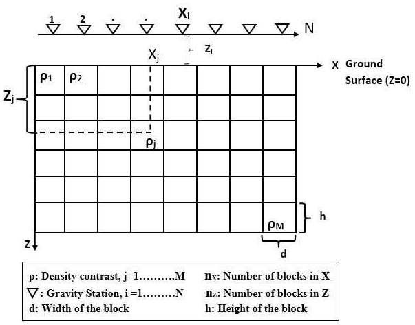
Figure 1 A 2D model of the subsurface under a gravity profile. Gravity stations (X_i) are located at the centers of the blocks, indicated by the ▽ symbols.

2.2 Forward modeling

After discretization of the modeling space into a set of elementary rectangular blocks, the total vertical-component gravity response calculated at the ith observation point g_i is the sum of the gravity contributions generated by each of the individual rectangular elements on all points belonging to the observation grid, and it is given by

$$\begin{array}{}\text{(1)}& g_i=\sum _{j=\mathrm{1}}^M{a}_{ij}{\mathit{\rho }}_j+e_{i}i=\mathrm{1},\mathrm{2},\mathrm{3}\mathrm{\dots }N,\end{array}$$

where ρ_j is the density of the jth prism, N denotes the numbers of observations, a_ij is the contribution of jth prism to the gravity value on ith observation point and e_i is the noise associated with ith data point. The kernel a_ij is the forward operator that maps from the physical parameter space to the data space. The exact mathematical expression of the kernel used here is presented by Last and Kubik (1983), which is adopted from Nagy (1966), to which the reader is referred for more detailed mathematical development. In matrix notation, Eq. (1) can be written as

$$\begin{array}{}\text{(2)}& \mathit{g}=\mathbf{A}\mathit{\rho }+\mathit{e},\end{array}$$

where g is an N-dimensional vector containing the gravity values, ρ is an M-dimensional model vector of densities, A is the N×M kernel matrix and e represents the noise vector at data points. Equation (2) constitutes the gravity forward modeling, that is used to calculate the predicted gravity anomalies (theoretical data) for a known subsurface density contrast (model ρ).

2.3 Inverse modeling

Our objective in solving gravity inverse problems is, given the observed gravity data (g), we seek a solution that gives a density distribution ρ which predicts the observed data with a certain noise level and, at the same time, satisfies certain constraints. For the model presented here, the density vector ρ is related to the predicted gravimetric field g by the linear expression given in Eq. (2). Like the majority of practical inverse problems arising in geophysical modeling, gravity inversion is an ill-posed problem. Moreover, usually we have a lesser number of observed gravity data than we do model parameters, which makes the system an under-determined problem. A standard way to solve such ill-posed and under-determined problems, according to regularization theory (Tikhonov et al., 2013), is minimization of the following objective function (Φ), which is the combination of data fidelity or the misfit functional (Φ_d) and stabilizing functional (stabilizer) terms (S(ρ)):

$$\begin{array}{}\text{(3)}& \mathrm{\Phi }={\mathrm{\Phi }}_{\mathrm{d}}+{\mathrm{\ell }}^{\mathrm{2}}S\left(\mathit{\rho }\right).\end{array}$$

Here, the misfit functional is ${\mathrm{\Phi }}_{\mathrm{d}}=\left|\right|{\mathbf{W}}_{\mathrm{e}}(\mathbf{A}\mathit{\rho }-{\mathit{g}}^{\mathrm{obs}})|{|}_{\mathrm{2}}^{\mathrm{2}}$, and W_e is the error-weighting diagonal matrix. In Eq. (3), ℓ is a regularization parameter that controls the trade-off between the data fidelity and the stabilizing term. Choosing a small value improves the data fit, but the recovered models have highly oscillatory artificial structures (which is equivalent to under-regularization). On the other hand, a large value of ℓ leads to a large misfit value between the observed and predicted data and a small norm of the model (over-regularizing the solution). Thus, the choice of a suitable value for ℓ is very important.

The choice of the stabilizing functional, in Eq. (3), depends on the desired model features that are to be recovered. There are several types of stabilizers that have been developed and implemented in the inversion of potential field data, which can roughly be divided into two categories: (I) smooth stabilizers, which use the L₂-norm of the model parameters or the gradient of the model parameters (Li and Oldenburg, 1998; Cella and Fedi, 2012; Paoletti et al., 2013); (II) non-smooth stabilizers, which use the L₁-norm or L₀-norm directly on the model parameters or on the gradient of the model parameters (Bertete-Aguirre et al., 2002; Sun and Li, 2014; Li et al., 2018; Utsugi, 2019). Inversion methods that utilize a smooth stabilizer produce models typically characterized by smooth features and hence have difficulties in recovering blocky structures or non-smooth distributions that have sharp boundaries or abrupt changes in physical properties (Farquharson, 2008). To overcome this problem, non-smooth stabilizers that help to produce compact and sharp models have been applied successfully (Zhdanov, 2009; Meng et al., 2018). Since we are interested in developing a gravity inversion method that can produce compact and sharp models, we use a non-smooth stabilizer through the L₀-norm on the model parameters, which will be discussed in the next subsection. In general, with all mentioned stabilizers, Eq. (3) needs to be solved by using an iterative minimization algorithm. In this work, we use the IRLS algorithm to estimate the solution, and it is described below.

Using the classical weighted L₂-norm stabilizing functional $S\left(\mathit{\rho }\right)=\left|\right|{\mathbf{W}}_{\mathrm{c}}(\mathit{\rho }-{\mathit{\rho }}_{\mathrm{F}})|{|}_{\mathrm{2}}^{\mathrm{2}}$ in the objective function Φ (Eq. 3) and minimizing by applying the standard weighted–damped least-squares optimization, the estimated density distribution in matrix notation can be given by the following (Menke, 1989, p. 55):

$$\begin{array}{}\text{(4)}& {\mathit{\rho }}^{k+\mathrm{1}}={\mathit{\rho }}_{\mathrm{F}}^k+\left[[{\mathbf{W}}_{\mathrm{c}}^k{]}^{-\mathrm{1}}{\mathbf{A}}^{\mathrm{T}}{\left(\mathbf{A}[{\mathbf{W}}_{\mathrm{c}}^k{]}^{-\mathrm{1}}{\mathbf{A}}^{\mathrm{T}}+{\mathrm{\ell }}^{\mathrm{2}}[{\mathbf{W}}_{\mathrm{e}}^k{]}^{-\mathrm{1}}\right)}^{-\mathrm{1}}{\mathit{g}}_{\mathrm{r}}^k\right],\end{array}$$

where the superscript k denotes that variable at kth iteration, and ${\mathbf{W}}_{\mathrm{c}}^k$ is a combined weighting matrix; ${\mathit{\rho }}_{\mathrm{F}}^k$ is reference density vector, which is from prior information or is calculated at each iteration; ${\mathit{g}}_{\mathrm{r}}^k={\mathit{g}}^{\mathrm{obs}}-\mathbf{A}{\mathit{\rho }}_{\mathrm{F}}^k$ represents the residual data vector computed at each iteration. Computation of the regularization parameter ℓ in Eq. (4) will be described in Sect. 2.3.3. In this work, the combined weighting matrix $\left({\mathbf{W}}_{\mathrm{c}}^k\right)$ is defined as a product of three different diagonal matrices: L₀-norm constraint matrix $\left({\mathbf{W}}_{L_{\mathrm{0}}}^k\right)$, depth weighting (W_z) and hard constraint matrix $\left({\mathbf{W}}_{\mathrm{h}}^k\right)$.

$$\begin{array}{}\text{(5)}& {\mathbf{W}}_{\mathrm{c}}^k={\mathbf{W}}_{L_{\mathrm{0}}}^k{\mathbf{W}}_z{\mathbf{W}}_{\mathrm{h}}^k\end{array}$$

2.3.1 L₀-norm constraint

The L₀-norm is commonly defined as the number of non-zero elements in a vector. Because there is no analytical formula that meets the mathematical requirement to be regarded as L₀-norm, the approximate expression is usually used to convert the L₀-norm into an equivalent norm for the suitability of computation. In the literature (Zhao et al., 2016; Li and Yao, 2020) that discusses the inversion of potential field data, different L₀-norm approximate stabilization functions have been developed and implemented to obtain focused images and sharp boundaries. Meng (2016) used a hyperbolic tangent function to approximate the L₀-norm and applied it to the 3D inversion of gravity gradient tensor data. Meng et al. (2018) proposed an exponential mathematical function to approximate the L₀-norm for 3D gravity sparse inversion. In this paper, the minimum-support functional, which is also called the compactness constraint, originally proposed by Last and Kubik (1983) and then further extended by Portniaguine and Zhdanov (1999) to include a reference model, is selected and can be expressed as follows:

$$\begin{array}{}\text{(6)}& L_{\mathrm{0}}\left(\mathit{\rho }\right)=\sum _{j=\mathrm{1}}^M{\displaystyle \frac{({\mathit{\rho }}_j-{\mathit{\rho }}_j^{\mathrm{apr}}{)}^{\mathrm{2}}}{({\mathit{\rho }}_j-{\mathit{\rho }}_j^{\mathrm{apr}}{)}^{\mathrm{2}}+\mathit{\epsilon }}}.\end{array}$$

In our case, to avoid the requirement of a prior model, we set ${\mathit{\rho }}_j^{\mathrm{apr}}=\mathrm{0}$, and hence, Eq. (6) can be rewritten as follows (Sun and Li, 2014):

$$\begin{array}{}\text{(7)}& L_{\mathrm{0}}\left(\mathit{\rho }\right)=\sum _{j=\mathrm{1}}^M{\displaystyle \frac{{\mathit{\rho }}_j^{\mathrm{2}}}{{\mathit{\rho }}_j^{\mathrm{2}}+\mathit{\epsilon }}},\end{array}$$

where ε is a focusing parameter. Application of L₀(ρ) as L₀(ρ) as a stabilizer in the minimization process of the objective function (Eq. 3) leads to the following choice of an L₀-norm constraint matrix $W_{L_{\mathrm{0}}}$, which is given by (Last and Kubik, 1983):

$$\begin{array}{}\text{(8)}& [{\mathbf{W}}_{L_{\mathrm{0}}}{]}_j=([{\mathit{\rho }}_j{]}^{\mathrm{2}}+\mathit{\epsilon }{)}^{-\mathrm{1}}.\end{array}$$

Based on Eq. (8), the kth iteration diagonal elements of the L₀-norm constraint matrix (${\mathbf{W}}_{L_{\mathrm{0}}}^k$) can be formulated as follows:

$$\begin{array}{}\text{(9)}& [{\mathbf{W}}_{L_{\mathrm{0}}}^k{]}_{jj}^{-\mathrm{1}}=[{\mathit{\rho }}_j^{k-\mathrm{1}}{]}^{\mathrm{2}}+\mathit{\epsilon }.\end{array}$$

The focusing parameter ε is a very important parameter. Its main purpose is to avoid singularities when ρ_j→0. The parameter ε is a small number, and in general, we are interested in the case where ε→0 because a small value leads to very compact models. However, this may introduce instability. On the other hand, if ε has a large value, the L₀-norm compactness constraint has no influence on the compactness of the model, which means it results in a smooth solution. Figure 2 shows the comparison of the minimum-support stabilizing functional for different values of ε to demonstrate the impact of the choice of different values of ε further. From Fig. 2, one can see that as ε becomes larger, the minimum-support stabilizing function loses its property and behaves more like the minimum-length L₂-norm stabilizer, which results in undesirable smoothness in the model, though it improves the stability. Therefore, it is essential to choose an optimal value of ε.

Figure 2 Comparison of the minimum-support stabilizing function for different values of ε.

In previous investigations, e.g., Last and Kubik (1983) and Guillen and Menichetti (1984), the parameter ε was assigned a value close to machine precision ($\approx {\mathrm{10}}^{-\mathrm{11}}$ to 10⁻¹⁵). Alternatively, Zhdanov and Tolstaya (2004) introduced a trade-off curve method, similar to the L-curve technique, to select ε by computing the model objective for the current model estimate over a range of values for ε. However, as pointed out by Ajo-Franklin et al. (2007), setting ε to values near machine precision results in severe instability, as ρ_j→0 and the approach of Zhdanov and Tolstaya (2004) often yield trade-off curves with corners that are not well defined. Therefore, it is better to fix ε at a reasonable value determined by experience, typically between 10⁻⁴ to 10⁻⁷ (Ajo-Franklin et al., 2007). Accordingly, in the present work, based on several numerical simulation tests, the value 10⁻⁶ is assigned just for the inversion examples presented in the paper. Note that the developed method is flexible regarding the use of different values of ε.

2.3.2 Error weighting

According to the compact inversion method proposed by Last and Kubik (1983), the kth-iteration error-weighting matrix ${\mathbf{W}}_{\mathrm{e}}^k$ is defined as

$$\begin{array}{}\text{(10)}& [{\mathbf{W}}_{\mathrm{e}}^k{]}^{-\mathrm{1}}=\mathrm{diag}\left(\mathbf{A}[{\mathbf{W}}_{L_{\mathrm{0}}}^k{]}^{-\mathrm{1}}{\mathbf{A}}^{\mathrm{T}}\right).\end{array}$$

Even though ${\mathbf{W}}_{\mathrm{e}}^k$, expressed by Eq. (10), is applied by many authors (Guillen and Menichetti, 1984; Barbosa and Silva, 1994; Ghalehnoee et al., 2017; Gebre and Lewi, 2022), some instability was reported by Lewi (1997, p. 87) in using ${\mathbf{W}}_{\mathrm{e}}^k$ in scenarios such as complicated geological geometry and when the data are contaminated with noise. To overcome this problem, Lewi (1997, p. 90) proposed a weighting matrix that makes use of the following equation:

$$\begin{array}{}\text{(11)}& [{\mathbf{W}}_{\mathrm{e}}^k{]}^{-\mathrm{1}}=\left[{\displaystyle \frac{[{\mathit{\sigma }}_{\mathit{\rho }}^{\mathrm{2}}{]}^k}{\mathrm{1}+[{\mathit{\sigma }}_{\mathrm{e}}^{\mathrm{2}}{]}^k}}\right]\mathbf{I},\end{array}$$

where I represents identity matrix, and ${\mathit{\sigma }}_{\mathit{\rho }}^{\mathrm{2}}$ and ${\mathit{\sigma }}_{\mathrm{e}}^{\mathrm{2}}$ are model and error variances, respectively, that are given by

$$\begin{array}{}\text{(12)}& {\displaystyle }[{\mathit{\sigma }}_{\mathrm{e}}^{\mathrm{2}}{]}^k={\displaystyle \frac{{\sum }_{i=\mathrm{1}}^N\mathit{\{}{\mathit{g}}_i-{\sum }_{j=\mathrm{1}}^M{a}_{ij}[{\mathit{\rho }}_j^{k-\mathrm{1}}]{\mathit{\}}}^{\mathrm{2}}}{N-\mathrm{1}}},\text{(13)}& {\displaystyle }[{\mathit{\sigma }}_{\mathit{\rho }}^{\mathrm{2}}{]}^k={\displaystyle \frac{{\sum }_{j=\mathrm{1}}^M[{\mathit{\rho }}_j^{k-\mathrm{1}}{]}^{\mathrm{2}}}{M-\mathrm{1}}}.\end{array}$$

The term in square brackets in Eq. (11) can be considered as the regularization parameter (Silva and Barbosa, 2006; Lewi, 1997, p. 90). Based on several numerical experiments done in the present work, it was observed that this term can sometimes end up with a larger value, which may result in over-regularization of the solution. For this reason, in the present study, a new error-weighting matrix ${\mathbf{W}}_{\mathrm{ne}}^k$ is introduced, and it is given as:

$$\begin{array}{}\text{(14)}& [{\mathbf{W}}_{\mathrm{ne}}^k{]}^{-\mathrm{1}}=\mathrm{diag}\left(\mathbf{A}\left[{\mathbf{W}}_z\left({\displaystyle \frac{[{\mathit{\sigma }}_{\mathit{\rho }}^{\mathrm{2}}{]}^k}{\mathrm{1}+[{\mathit{\sigma }}_{\mathrm{e}}^{\mathrm{2}}{]}^k}}\right){\mathbf{W}}_{\mathrm{h}}^k\right]{\mathbf{A}}^{\mathrm{T}}\right).\end{array}$$

Let us represent the terms in square brackets by ${\mathbf{W}}_n^k$ as follows:

$$\begin{array}{}\text{(15)}& {\mathbf{W}}_n^k={\mathbf{W}}_z\left({\displaystyle \frac{[{\mathit{\sigma }}_{\mathit{\rho }}^{\mathrm{2}}{]}^k}{\mathrm{1}+[{\mathit{\sigma }}_{\mathrm{e}}^{\mathrm{2}}{]}^k}}\right){\mathbf{W}}_{\mathrm{h}}^k,\end{array}$$

where W_z and ${\mathbf{W}}_{\mathrm{h}}^k$ are diagonal depth and hard constraint matrices respectively; these will be described in the next subsections. Then the error-weighting matrix in Eq. (14), the one introduced and implemented here, becomes

$$\begin{array}{}\text{(16)}& [{\mathbf{W}}_{\mathrm{ne}}^k{]}^{-\mathrm{1}}=\mathrm{diag}\left({\mathbf{AW}}_n^k{\mathbf{A}}^{\mathrm{T}}\right).\end{array}$$

2.3.3 Auto-adaptive regularization parameter estimation

Choosing a suitable value for the regularization parameter is a crucial part of the inversion process. The precise value of the regularization parameter depends on the noise level associated with the observed data. Thus, the higher value of ℓ refers to the higher noise level of the data points. Several methods have been proposed to choose the appropriate value of regularization parameter and are reviewed in the literature (Farquharson and Oldenburg, 2004; Vatankhah et al., 2014) and standard texts, for example, Vogel (2002, pp. 97–109) and Aster et al. (2018, p. 57). In particular, depending on the noise level, a constant value of ℓ, throughout the inversion, has been chosen by many authors (Silva and Barbosa, 2006; Ghalehnoee et al., 2017). In other works (for example, Zhdanov (2009) and Rezaie et al. (2017)), the parameter ℓ has been iteratively updated in each iteration.

As pointed out in previous works (Farquharson and Oldenburg, 2004; Gholami and Aghamiry, 2017), instead of using a constant value of ℓ, dynamic re-adjustment throughout the iterative scheme might be a superior approach. Taking this into account, in the present work, ℓ is updated in each iterative step. In our implementation, to select an optimal regularization parameter at each iteration, we proposed an auto-adaptive regularization method. This method leads to an automatic update of the regularization parameter at each and every iteration. The basic principle, including its procedure in relation to the formally known adaptive regularization approach, which was proposed by Zhdanov (2002, p. 55) and has been implemented by many authors (Zhdanov, 2009; Rezaie et al., 2017), is as follows. In the adaptive regularization approach, the initial value of the regularization parameter ℓ¹ is updated at each iteration step by Zhdanov (2002, p. 55):

$$\begin{array}{}\text{(17)}& {\mathrm{\ell }}^k={\mathrm{\ell }}^{\mathrm{1}}{q}^k,\end{array}$$

where q, as described by Zhdanov (2002, p. 55), is the damping factor which decreases from iteration to iteration. Its initial value is empirically determined, having a value between 0 and 1. It is obvious that the trial-and-error selection of the value for q requires computational work . The presented auto-adaptive regularization method overcomes this problem, and the iterative values ℓ^k are determined by the following formula:

$$\begin{array}{}\text{(18)}& {\mathrm{\ell }}^k={\mathrm{\ell }}^{k-\mathrm{1}}\left[{\displaystyle \frac{|{\mathit{g}}^{\mathrm{obs}}-\mathbf{A}\mathit{\rho }{|}_{\max }^{k-\mathrm{1}}}{|{\mathit{g}}^{\mathrm{obs}}-\mathbf{A}\mathit{\rho }{|}_{\max }^k}}\right],\end{array}$$

where the term in the square bracket is an adjusting factor that is automatically determined at each iterative step, and $|{\mathit{g}}^{\mathrm{obs}}-\mathbf{A}\mathit{\rho }{|}_{\max }$ is the maximum absolute value of the residual data elements. In the auto-adaptive regularization method, choosing a suitable initial value of (ℓ_o) is essential. Based on a number of synthetic and real data simulations done in this work, we recommend the following in choosing a reasonable value of ℓ_o. Firstly, the initial value of ℓ should be within the range $\mathrm{0}<{\mathrm{\ell }}_{\mathrm{o}}\le \mathrm{1}$. Secondly, the precise value of ℓ_o depends on the noise level related to the observed data. When the probable or expected noise level of the data is higher, a larger value ℓ_o is a reasonable choice to avoid unwanted and false anomalies due to noise. In contrast, when the probable or expected noise level is less, a small value of ℓ_o should be chosen. Once an appropriate initial value ℓ_o is given as an input, Eq. (18) is used to determine ℓ^k for subsequent iterations. The advantage of the auto-adaptive regularization scheme is its capability to automatically determine a suitable regularization parameter in the course of the optimization process, depending on the automatically determined adjusting factor.

2.3.4 Physical parameter constraint

To produce a physically meaningful model from a gravity inverse solution, the usage of lower- and upper-bound constraints on the recovered density contrast is beneficial (Silva et al., 2001; Grandis and Dahrin, 2014). Lower and upper bounds can be obtained from a priori information such as geological investigations in conjunction with published density values of rocks, well logging and/or laboratory tests. Many procedures such as the gradient projection approach (Wang and Ma, 2007; Lelièvre et al., 2009), transform function approach (Pilkington, 2008) and logarithmic barrier approach (Li and Oldenburg, 2003) have been applied in different inversion schemes to implement this constraint. However, with regard to the L₀-norm-stabilizer-based gravity inversion methods, an effective method is the direct utilization of lower and upper density constraints (Meng et al., 2018). Hence, in this work, the direct density bound inequality constraint is used – that is, at each iteration, the density contrast of each rectangular block is bounded by the minimum and maximum density constraint function given by

$$\begin{array}{}\text{(19)}& [{\mathit{\rho }}^k{]}_j=\left\{\begin{array}{l}\left[{\mathit{\rho }}_{\max }{]}_j\text{if}\right[{\mathit{\rho }}^k{]}_j>[{\mathit{\rho }}_{\max }{]}_j\\ \left[{\mathit{\rho }}^k{]}_j\text{if}\right[{\mathit{\rho }}_{\min }{]}_j<[{\mathit{\rho }}^k{]}_j<[{\mathit{\rho }}_{\max }{]}_j\\ \left[{\mathit{\rho }}_{\min }{]}_j\text{if}\right[{\mathit{\rho }}^k{]}_j<[{\mathit{\rho }}_{\min }{]}_j\end{array}.\right.\end{array}$$

By using this function, if kth iteration ρ_j of any block exceeds one of its bounds, then it will be fixed at the violated bound.

In each iteration step, the procedure to compute the hard constraint matrix ${\mathbf{W}}_{\mathrm{h}}^k$ (Boulanger and Chouteau, 2001) and the reference density vector ${\mathit{\rho }}_{\mathrm{F}}^k$ is determined as follows. The diagonal elements of ${\mathbf{W}}_{\mathrm{h}}^k$ are fixed at ε or 1.0. When a priori geological and geophysical information is able to provide the initial value of the density contrast of the jth specific cells, then these values are assigned to the corresponding $[{\mathit{\rho }}_{\mathrm{F}}^k{]}_j$. Simultaneously, the corresponding diagonal elements of $[{\mathbf{W}}_{\mathrm{h}}^k{]}_{jj}$ are set to be ε. During the inversion process, if the jth elements of estimated density values fall out of the inequality constraint limits defined by ρ_min and ρ_max, then $[{\mathit{\rho }}_{\mathrm{F}}^k{]}_j$ will be fixed at the violated bound density itself, and $[{\mathbf{W}}_{\mathrm{h}}^k{]}_{jj}$ will be assigned to be ε. On the other hand, if the elements of the estimated density did not exceed its bounds (i.e., they lie between the limits), $[{\mathbf{W}}_{\mathrm{h}}^k{]}_{jj}$ and $[{\mathit{\rho }}_{\mathrm{F}}^k{]}_j$ are assigned to be 1.0 and 0.0 respectively.

Using ${\mathbf{W}}_{\mathrm{h}}^k$, any blocks with a density known from a priori information or exceeding the density constraint limit will be automatically frozen by the algorithm in the next iteration by having a very small weight assigned to it, and ${\mathit{\rho }}_{\mathrm{F}}^k$ is used to remove the gravity effects of those cells that have crossed the inequality constraint limit from the observed gravity data. That is applied to compute the reduced-gravity data vector ${\mathit{g}}_{\mathrm{r}}^k={\mathit{g}}^{\mathrm{obs}}-\mathbf{A}{\mathit{\rho }}_{\mathrm{F}}^k$ in Eq. (4) of the inversion algorithm. In other words, at each iterative step, the inversion of subsequent iterations will be performed using the reduced-gravity data vector.

2.3.5 Depth weighting

It is well known that gravity data, like any potential field data, have no inherent depth resolution. The model structures reconstructed by the inversion process tend to concentrate near the surface regardless of the true depth of the causative bodies (Li and Oldenburg, 1996). This happens because the inverse solution of model construction is a linear combination of kernels, whose amplitudes rapidly decay with depth. The problem can be overcome by introducing a depth-weighting matrix to counteract the natural decay of kernels with depth (Li and Oldenburg, 1998). Depth weighting is designed to ensure that all cells have equal likelihood of accommodating the sources, not just those at shallow levels that are most sensitive to the observed data. Depth weighting is used and its effect is investigated by different authors (Pilkington, 2008; Commer, 2011). Based on Gebre and Lewi (2022), the recently proposed depth-weighting function is given as follows:

$$\begin{array}{}\text{(20)}& w_{zj}=(a{Z}_j+c_{\mathrm{o}}{)}^{-\mathit{\tau }},\end{array}$$

where Z_j is the mean depth of the jth cell, and a, c_o and τ are adjustable parameters. The values of the three adjustable parameters are computed by optimizing w_z(z) to match with the actual gravity kernel values utilizing nonlinear least-squares minimization (Virtanen et al., 2020). Accordingly, for all inversions in this work, the depth-weighting matrix similar to the one used by Gebre and Lewi (2022) is employed (Eq. 21):

$$\begin{array}{}\text{(21)}& [{\mathbf{W}}_z{]}_{jj}=\mathbf{diag}(w_{zj}),\end{array}$$

where W_z is diagonal M×M depth-weighting matrix.

2.3.6 Stopping criteria

It is clear that if the iterations are stopped too early, then a reasonable solution of the inverse problem may not be obtained. On the other hand, too many iterations may waste computer time without increasing the overall solution qualities. Thus, an important aspect of any iterative inversion method is to decide when the iterations should be terminated. A number of stopping criteria have been proposed and employed to terminate iterative inversion algorithms (Borges et al., 2015; Levin and Meltzer, 2017). Commonly used stopping criteria are based on a norm of the residual vector (i.e., the norm of the difference between estimated and observed data). For instance, a noise level, i.e., ${\mathit{\chi }}^{\mathrm{2}}=\left|\right|{\mathbf{W}}_{\mathrm{d}}({\mathit{g}}^{\mathrm{obs}}-\mathbf{A}\mathit{\rho })|{|}_{\mathrm{2}}^{\mathrm{2}}$, where a diagonal data-weighting matrix W_d, whose ith element is the inverse of the standard deviation of the noise at each data point, is used by Boulanger and Chouteau (2001) and by Vatankhah et al. (2017). Other criteria for stopping the gravity inversion procedure are based on simple misfit or the root-mean-square error (RMSE) between the observed data and predicted data produced by the recovered model (see, for example, Rezaie and Moazam, 2017). The expressions used to estimate these criteria are the following:

$$\begin{array}{}\text{(22)}& {\displaystyle }\mathrm{misfit}={\left({\displaystyle \frac{{\sum }_{i=\mathrm{1}}^N({\mathit{g}}_i^{\mathrm{obs}}-{\mathit{g}}_i^{\mathrm{cal}}{)}^{\mathrm{2}}}{{\sum }_{i=\mathrm{1}}^N({\mathit{g}}_i^{\mathrm{obs}}{)}^{\mathrm{2}}}}\right)}^{\frac{\mathrm{1}}{\mathrm{2}}},\text{(23)}& {\displaystyle }\mathrm{RMSE}={\displaystyle \frac{\left({\sum }_{i=\mathrm{1}}^N\right({\mathit{g}}_i^{\mathrm{obs}}-{\mathit{g}}_i^{\mathrm{cal}}{)}^{\mathrm{2}}{)}^{\frac{\mathrm{1}}{\mathrm{2}}}}{N}},\end{array}$$

Ekinci (2008) also introduced another possible criterion, namely the parameter variation function (smy), which is defined as follows:

$$\begin{array}{}\text{(24)}& \mathrm{smy}={\left(\sum _{j=\mathrm{1}}^M({\mathit{\rho }}_j^k-{\mathit{\rho }}_j^{k-\mathrm{1}}{)}^{\mathrm{2}}\right)}^{\frac{\mathrm{1}}{\mathrm{2}}}.\end{array}$$

The most widely used approach is to quit the iterative process when one of the above criteria are below a given tolerance (the level of observational error). However, in practical applications, a precise value for such tolerance is rarely known; rather, only some possibly vague idea of the desired quality of the numerical approximation is at hand. Moreover, it has been pointed out by Rao et al. (2018) that stopping iteration based solely on the norm of the residual is neither safe nor a robust solution. The non-uniqueness and instability of the gravity inverse problem further complicates the usage of only one of the aforementioned stopping criteria. To overcome these issues, a combination of the misfit and smy has been utilized in this paper. Therefore, the iterative procedure continues until one of the following stopping criteria is met: (I) the maximum number of iterations (k_max) given by the user is reached, or (II) the difference between two consecutive iteration values of smy and misfit have reached the target values. That means that for the second criterion, both the conditions $|{\mathrm{smy}}^{k-\mathrm{1}}-{\mathrm{smy}}^k|\le \mathit{\tau }$ and $|{\mathrm{misfit}}^{k-\mathrm{1}}-{\mathrm{misfit}}^k|\le \mathit{\mu }$ must be satisfied at the same time. In all demonstrations considered in this work, after testing different values, the parameter τ is assigned to $\sqrt{\mathrm{2}M}$, and μ is assigned to 0.005, where M is again the total number of model parameters. The effectiveness of the proposed termination criteria will be illustrated by using synthetic tests.

2.4 Computational procedure

The solution of the linear system of equations in Eq. (2) will be carried iteratively using the information about the misfit and density from successive iteration. The input parameters for the inversion procedure are as follows: (1) kernel matrix (A) and discretized subsurface model (mesh) and its initial approximation reference density model ρ_F if it exists based on a priori information; (2) observed gravity anomaly (g) at measurement points (x); (3) maximum number of iterations (k_max); (4) lower ρ_min and upper ρ_max density bounds and initial ℓ_o value. In summary, the steps taken to carry out the inversion process consist of the followings:

1. For k=0, if there is no a priori information, ${\mathbf{W}}_{L_{\mathrm{0}}}$, W_c, W_n and W_h are identity matrices, ρ_F=0. W_z and W_ne are computed through Eqs. (21) and (16) respectively; after this, the first-iteration model parameters solution is obtained by Eq. (4).

2. The elements of W_h and ρ_F are updated as explained in the preceding section, then ${\mathbf{W}}_{L_{\mathrm{0}}}$ is calculated using Eq. (9), and then W_c is calculated using Eq. (5).

3. The values of σ_ρ and σ_e are computed using Eqs. (13) and (12) respectively. Then W_n is calculated using Eq. (15).

4. To remove the effect of those blocks that have crossed the maximum target density, evaluate the reduced data ${\mathit{g}}_{\mathrm{r}}^k={\mathit{g}}^{\mathrm{obs}}-\mathbf{A}{\mathit{\rho }}_{\mathrm{F}}^k$. Then compute the current ℓ with Eq. (18) and W_ne with Eq. (16).

5. The inversion is carried out through Eq. (4).

6. Application of inequality constraints on density are carried out as discussed in the preceding section.

7. Now a forward-modeling procedure will be carried out using Eq. (2) to compute the gravity anomaly g^cal from the estimated model in the previous iteration.

8. Data misfit (Eq. 22) and smy (Eq. 24) are computed using g^cal from step 7 and the obtained model parameters from the previous and current iteration.

9. Testing is carried out to confirm if the stopping criteria are fulfilled. If the termination criteria are satisfied, the iteration terminates, and obtained results are stored and plotted. Otherwise, using the current estimated density model, move to the next iteration k by going to the second step and continue the iterative procedure until the stopping criteria are fulfilled.

3 Synthetic model test

To evaluate the functionality and efficiency of the method, the developed procedure was tested on several synthetic model examples. The examples presented here are randomly chosen to demonstrate the following: (I) the applicability of the proposed auto-adaptive regularization technique (Eq. 18) and error-weighting function (Eq. 16); (II) the performance of the method in producing compact and sharp images of the causative bodies; (III) the effectiveness of the combined stopping criterion. The forward and the inverse problem were carried out using the procedure described in the preceding sections. In the inversion of the synthetic examples, the same subsurface discretization as the one used in generating the synthetic data (forward modeling) is used. All the inversion tests are performed on a desktop computer (11th Gen Intel(R) Core(TM) i7-11700, 2.50 GHz processor). For the first and second synthetic examples presented in this work, (I) the model region was discretized into 60 × 15 rectangular cells, and the dimensions of each cell were taken as 10 × 10 m in the x and y directions respectively; (II) the synthetic gravity data were computed at 60 data points that are centered in each cell at the top side of the model to produce data at a 10 m sample interval; (III) the computed gravity data are contaminated with Gaussian noise that has a standard deviation that amounts to 4 % of the magnitude at each data point with zero mean (Farquharson, 2008; Rezaie et al., 2017).

The first synthetic data inversion has been done for the model presented in Fig. 3a. For this synthetic model, the causative bodies are two rectangular structures elongated differently in the horizontal and vertical directions and located at different depths. The causative bodies have the same density contrast of 1000 kg m⁻³. The density of the causative bodies are given relative to the zero density of uniform background. Figure 3a (upper panel) shows noise-free (solid line) and noise-contaminated (star dots) gravity data. Separate inversion runs for three different ℓ_o values (0.2, 0.3 and 0.4) were performed with the developed inversion method. Note that, for subsequent iterations, the proposed auto-adaptive regularization technique (Eq. 18) is used to compute ℓ for each case. At the beginning of the inversion, the iterations are initialized with ρ_F=0 and ${\mathbf{W}}_{\mathrm{h}}={\mathbf{W}}_{\mathrm{c}}={\mathbf{W}}_n={\mathbf{W}}_{L_{\mathrm{0}}}=\mathbf{I}$. The lower-limit density contrasts of all cells is zero (ρ_min=0), and the upper bound ρ_max=1000 kg m⁻³.

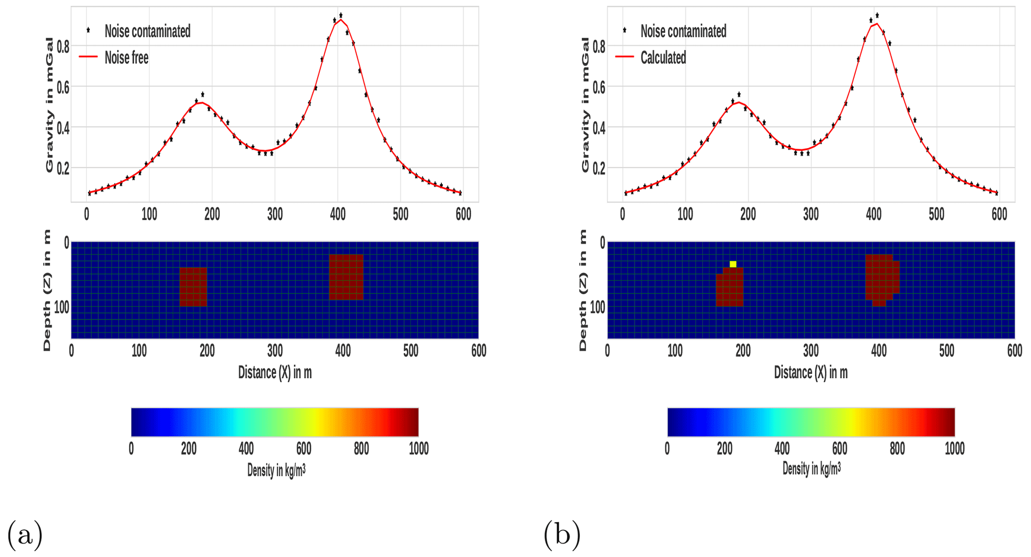
Figure 3 The first synthetic model and the result of the inversion. (a) The lower panel represents the 2D synthetic model, which constitutes two isolated rectangular bodies located at various depths, and the top panel shows the gravity anomaly due to these two subsurface rectangular bodies. (b) The lower panel represents the subsurface as a result of the proposed inversion method using ℓ_o=0.3, and the top panel shows the synthetic data together with the data derived from the model.

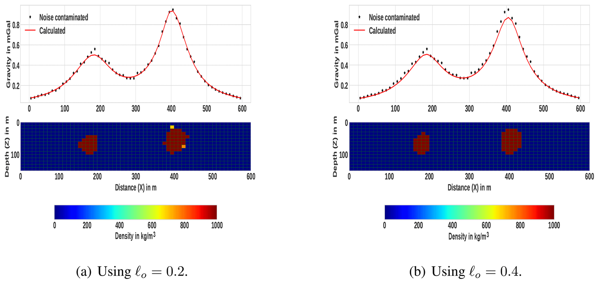
Figure 4 Inversion results, using different ℓ_o values, for the first synthetic model given in Fig. 3a.

The results of the inversion using the developed method for three different ℓ_o values are shown in Figs. 3b and 4. The corresponding data fit between the predicted (solid line) and the actual contaminated (stars) gravity data is also shown. Comparing the inversion results with the original synthetic model in Fig. 3a, the inversion has sufficiently recovered the true models. The depth, geometry and density distributions of the synthetic causative bodies were recovered adequately. This can confirm the applicability of the proposed auto-adaptive regularization technique (Eq. 18) and error-weighting function (Eq. 16). Notice that the results also indicate the robustness and stability of the developed inversion method for different ℓ_o values. The average computation time to finish the inversion is approximately 16.3 s.

The second synthetic model is more complicated and consists of two causative bodies placed at various depths. The bodies have different sizes, shapes and density contrasts. The first causative body is a vertical rectangular block, with density contrast 2000 kg m⁻³ and placed at 40 m depth, and the second body is a dipping dike, with density contrast 3000 kg m⁻³ at 20 m depth. The synthetic model is shown in the lower part of Fig. 5a, and the generated noise-corrupted and noise free-gravity data are shown on the upper part.

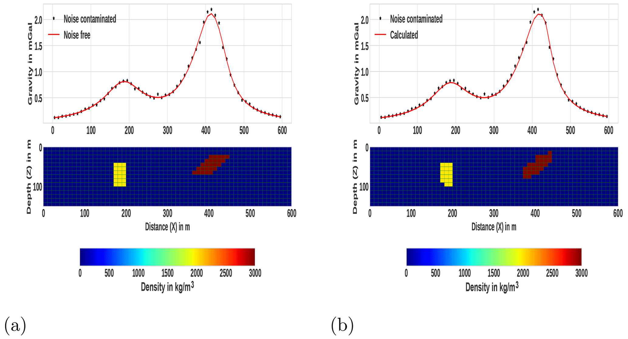
Figure 5 The second example synthetic model and the corresponding inversion result. (a) Synthetic model consisting of a dipping dike and vertical rectangular block and the corresponding gravity data. (b) The density model obtained by inverting the gravity data using the developed method. The predicted data as a result of inversion process are shown on the top panels (solid line).

Using the generated synthetic data, the inversion was initiated by assigning an initial zero density to each cell. We set initial ℓ_o=0.3. The density contrast limits are bounded between the lower bound ρ_min=0 and the upper bound ρ_max=3000 kg m⁻³. Even though a maximum iteration of 20 was set, the misfit and smy between two consecutive iterations gradually fell below the threshold set after the 14th iteration. The total computation time was approximately 15.73 s.

In Fig. 5b, the resulting model from the inversion of the second synthetic model (Fig. 5a) using the proposed method is presented. As can be seen in Fig. 5b (upper panel), the modeled gravity data (solid line) fit adequately with the synthetic data. The result, presented in Fig. 5b (lower panel), indicates an acceptable reconstruction of the synthetic multi-sources and multi-shape bodies that are located at different depths. The true shape, location and density of the causative bodies are recovered adequately. Like the first example, the reproduced images of the localized multiple sources are compact and sharp (Fig. 5b, lower panel).

For the third and fourth synthetic examples, (I) the subsurface model was discretized into 100 × 20 rectangular cells; each cell has a size of 50 m in x and z directions; (II) the synthetic gravity data were computed on 100 data points with a sample spacing of 50 m. The third synthetic model includes two dipping dikes in opposite directions. The causative 2D bodies have different sizes and the same density contrast that amounts to 1000 kg m⁻³ in a homogeneous-background zero density. The top part of the shallower dipping dike lies at a depth of 200 m, and that of the deeper dike lies at a depth of 250 m. The computed gravity data were contaminated by uncorrelated Gaussian noise whose standard deviation was equal to 4 % of the difference between the maximum and the minimum anomaly and zero mean. The synthetic model and the corresponding data are shown in Fig. 6 at the lower and upper panels respectively.

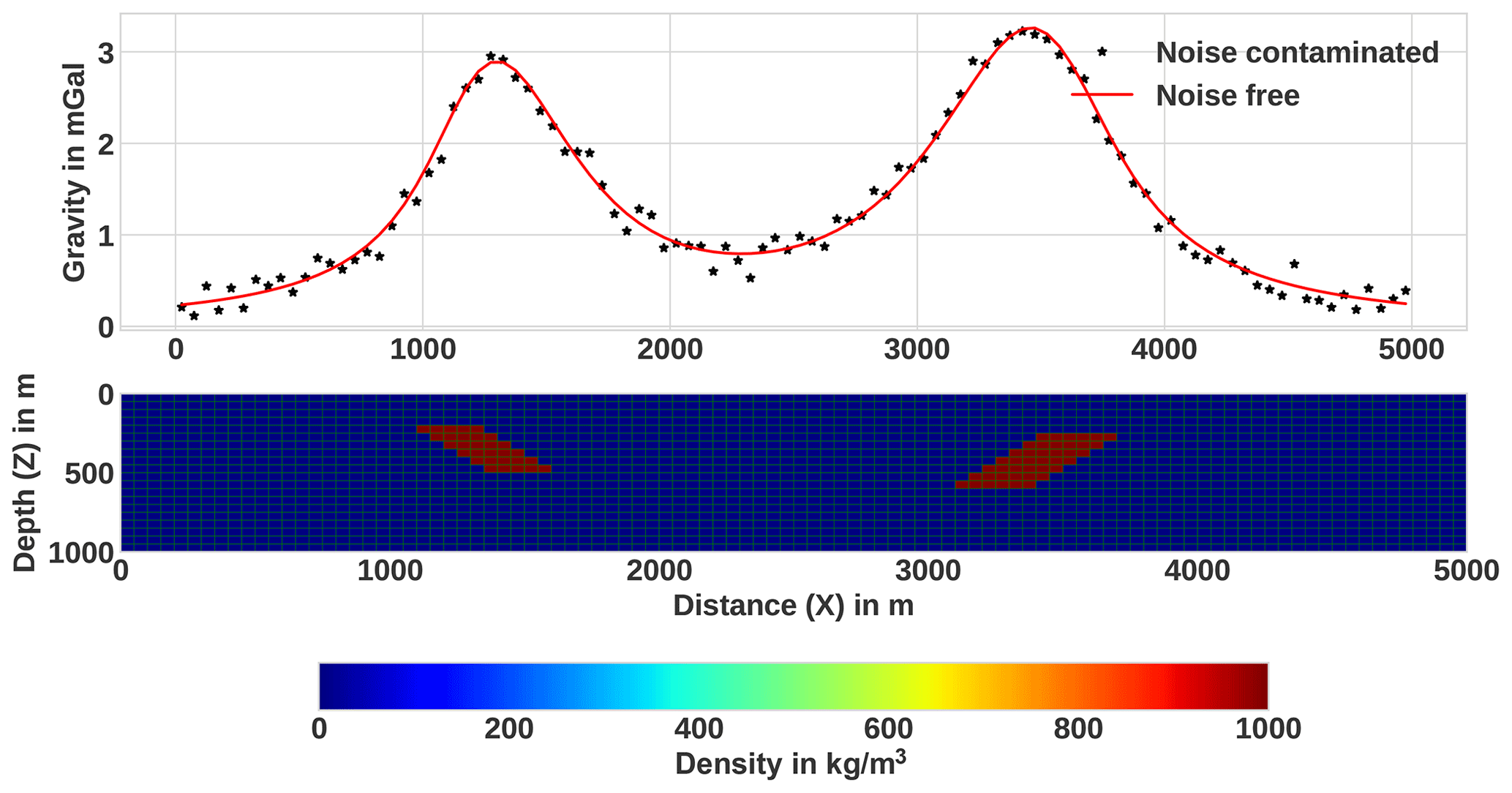
Figure 6 The third synthetic model that comprises two dikes at various depths, with the density contrast that amounts to 1000 kg m⁻³ and the corresponding gravity data.

The inversion process was commenced by setting the densities of all cells to zero. The initial value of ℓ_o was set to 0.4. The bounding density ranges were set to a minimum value ρ_min=0 and maximum value ρ_max=1000 kg m⁻³. The maximum number of iterations was set to 20. Here, the inversion converged after the 13th iteration, and the total computation time was approximately 66.49 s. The resulting model and the inverted data using the proposed method are shown in Fig. 7b. For the sake of comparison, keeping all inversion parameters the same, the synthetic data were also inverted with the classical L₂-norm-regularized inversion approach, and the obtained result is shown in Fig. 7a. As can be seen from the lower panel of Fig. 7b, unlike the model in Fig. 7a, the developed method was able to produce a compact and sharp model successfully. The other concern, which can be seen from the result in Fig. 7a, is that the target density contrast values are underestimated in the case of the conventional L₂-norm inversion. In contrast, the geometry, locations and densities of both anomalous structures were adequately recovered with the presented inversion method (see Fig. 7b).

Figure 7 Inversion results of the third synthetic example in Fig. 6 using (a) the conventional minimum norm (L₂-norm) smooth stabilizer and the corresponding data fit, and (b) the presented method.

The fourth synthetic model consists of two different rectangular, anomalous bodies (Fig. 8a, lower panel). The anomalous structures have different dimensions and are buried at different depths. The top of the first rectangular block is placed at a depth of 200 m, and its density contrast is −1000 kg m⁻³, while the top of the second block is placed at a depth of 250 m and has a density contrast of 1000 kg m⁻³. Different density contrast, size and depth of adjacent structures have been considered to show the ability of the presented inversion method in reconstructing true parameters for these models. In this synthetic example, the computed data are contaminated by Gaussian noise with a standard deviation of 3 % of the difference between the maximum and the minimum anomaly.

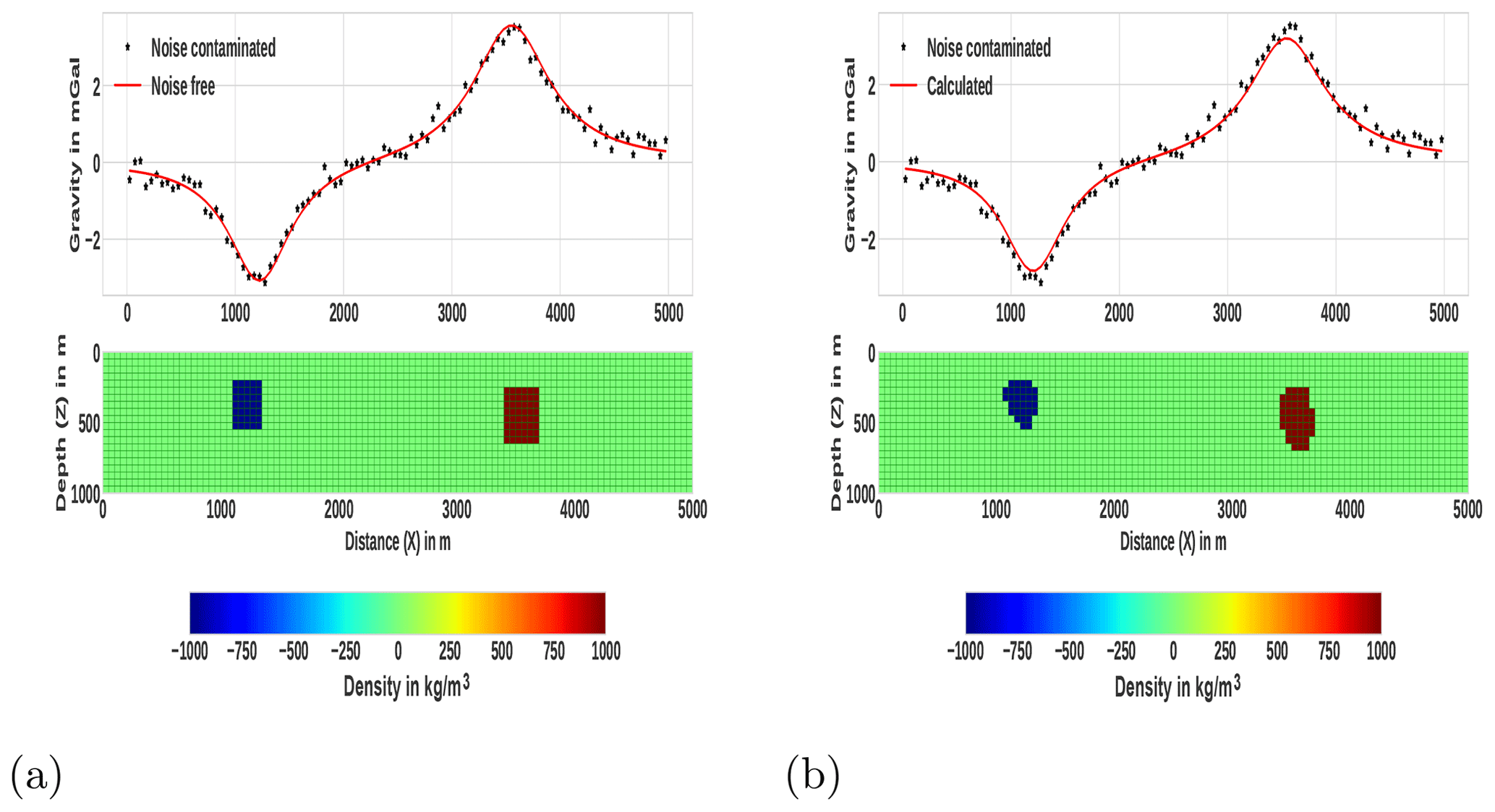
Figure 8 The fourth synthetic model example and the corresponding inversion result. (a) Synthetic model consisting of two rectangular bodies at various depths with different density contrasts and the corresponding noise-free and noise-contaminated gravity data. (b) The lower panel shows the recovered density contrast model obtained by inverting the gravity data using the developed method, while the upper one shows the associated fits between the synthetic data that are taken from (a) and the predicted response.

For the current example, the inversion process was initialized by setting the initial value of ℓ_o=0.5. The lower bound for the density constraint ${\mathit{\rho }}_{\min }=-\mathrm{1000}$ kg m⁻³, and the upper bound ρ_min=1000 kg m⁻³. Similar to the previous examples, though the maximum number of iterations was set to be 20, the iterative step terminated when the proposed combined criterion was satisfied after 11 iterations. The approximate running time required to finish the inversion was 55.64 s. Figure 8b lower panel shows the recovered density contrast model. The corresponding fits between synthetic (stars) and predicted data (line) are shown in the upper panel of the same figure. We can see that the recovered rectangular bodies are compact and have sharp boundaries. The obtained results also indicate that the depth and density contrast of the anomalous rectangular bodies have been determined sufficiently.

Here, the effectiveness and the advantage of the proposed combined stopping criterion are illustrated by comparing it with another commonly used stopping condition. For this reason, the inversion process was performed again with the developed inversion method using only the misfit function ($|{\mathrm{misfit}}^{k-\mathrm{1}}-{\mathrm{misfit}}^k|$) as a stopping condition. Note that, for comparison purposes, all the other inversion parameters are set to be the same, except for the stopping criterion. The resulting recovered density contrast models and the data fit are presented in Fig. 9. The corresponding values of the misfit and smy as a function of iteration number are also shown in Fig. 10a. For the sake of comparison, the misfit and smy when using the proposed combined stopping criterion for the same data set are also presented in Fig. 10b. The stopping condition $|{\mathrm{misfit}}^{k-\mathrm{1}}-{\mathrm{misfit}}^k|\le \mathit{\mu }$ was reached after 5 iterations, as shown in the curve of Fig. 10a, before the true density distribution had been recovered fully. In other words, the estimated models are not satisfactory because densities lower than the target density are observed around the edges of the anomalous bodies (Fig. 9). This indicates that, unlike the result presented in Fig. 8b, where the proposed combined stopping condition is used, quitting the iterative process only with $|{\mathrm{misfit}}^{k-\mathrm{1}}-{\mathrm{misfit}}^k|\le \mathit{\mu }$ criterion produces a premature solution – that is, before the maximum compactness is achieved.

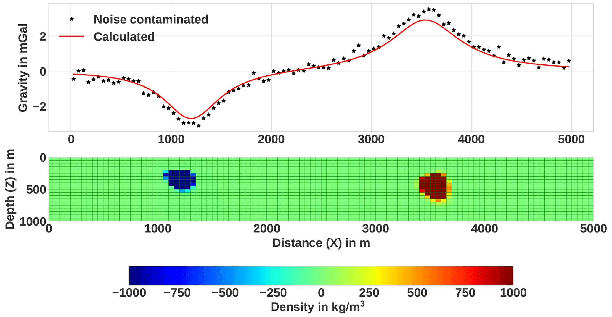
Figure 9 Inversion result obtained using only the commonly used criterion ($|{\mathrm{misfit}}^{k-\mathrm{1}}-{\mathrm{misfit}}^k|$) and the corresponding data fit (upper panels) for the synthetic example in Fig. 8a. The obtained density model shows that the compact and sharp model was not approximately achieved due to the termination before the iterative procedure had reached convergence.

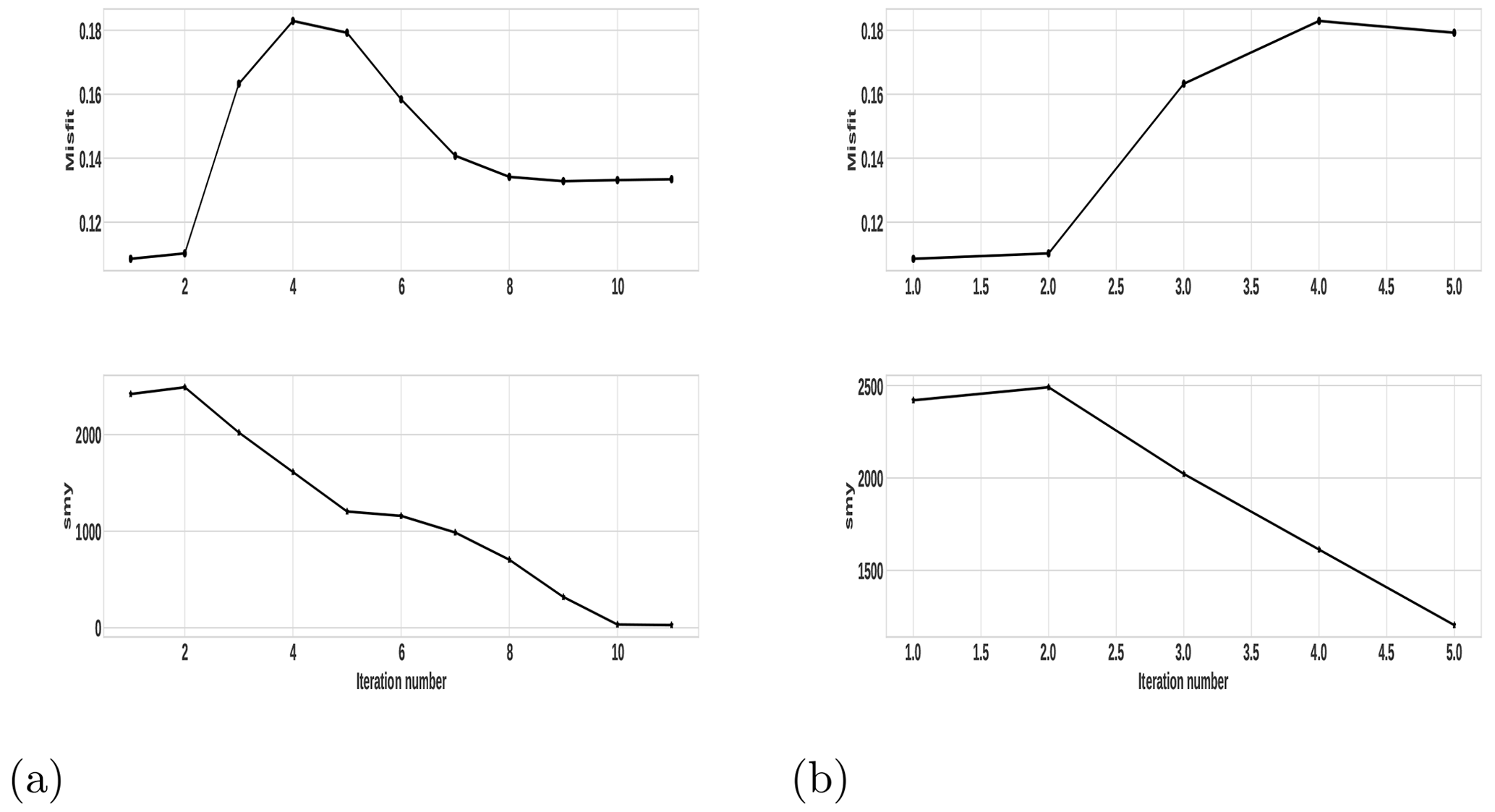
Figure 10 The progression of misfit and smy in the course of the iteration during the inversion of the fourth example's synthetic data (a) using the proposed combined stopping condition and (b) using only $|{\mathrm{misfit}}^{k-\mathrm{1}}-{\mathrm{misfit}}^k|\le \mathit{\mu }$.

A number of other numerical experiments we carried out showed that there are situations where either misfit^k| or $|{\mathrm{misfit}}^{k-\mathrm{1}}-{\mathrm{misfit}}^k|$ fall below the given threshold values, at earlier iterations, before the true density is fully recovered. Thus, it is hard to take only one criterion as a termination condition. As stated in Sect. 2.3.6, it has been mentioned that the same has also be pointed out in a number of previous works (Rao et al., 2018). On the other hand, in the case of the proposed criterion (that is, when both the conditions $|{\mathrm{smy}}^{k-\mathrm{1}}-{\mathrm{smy}}^k|\le \mathit{\tau }$ and $|{\mathrm{misfit}}^{k-\mathrm{1}}-{\mathrm{misfit}}^k|\le \mathit{\mu }$ are satisfied at the same time), the inversion process yields an acceptable model. This clearly illustrates the advantage of using the proposed stopping criterion and its effectiveness in quitting the iterative scheme after the optimal number of iterations.

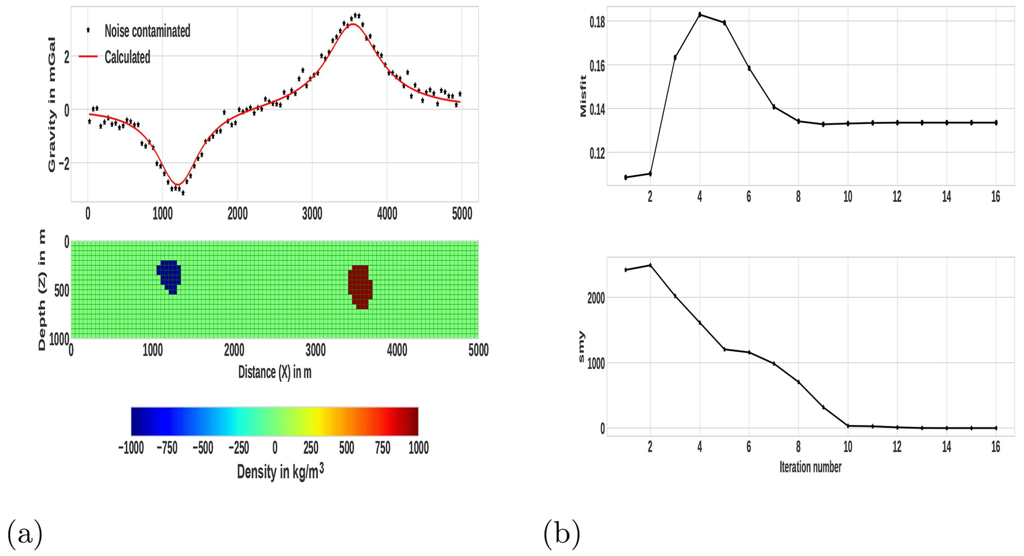
Figure 11 Late-iteration-termination (at 16th iteration) inversion result and the corresponding misfit and smy variations, with the iteration number for the fourth example in Fig. 8. (a) The obtained recovered density model (lower panel) and the corresponding data fit (upper panel). (b) Progression of misfit (top panel) and smy (lower panel) in the course of the iterative procedure.

To further illustrate the effectiveness of the proposed combined criterion, the inversion process is allowed to continue to the 16th iteration, and the model, as a result of this, is presented in Fig. 11a. The progressions of the misfit and smy in the course of the iterative procedure are also given in Fig. 11b. As can be seen from the result (Fig. 11b), the solution obtained at subsequent iterations after the 11th iteration, where the iteration is terminated with the proposed stopping condition, remains virtually unaltered. This can also be observed from the misfit and smy variation curves shown in Fig. 11b, such that after the 11th iteration the misfit and smy values remain literally unchanged. Moreover, the results also indicate the appropriateness of the suggested threshold values μ and τ used in the proposed stopping criterion. The other thing one can observe from the results in Fig. 11 is the stability of the developed inversion method. This can also illustrate the effectiveness of the newly proposed auto-adaptive regularization technique (Eq. 18) and error-weighting function (Eq. 16).

In general, the presented method was tested with noise-contaminated data that are generated from different geometries, locations, sizes and density contrasts of causative bodies, and it has successfully recovered all models. Moreover, all the reconstructed images of the presented synthetic models are compact and sharp. Numerous synthetic data inversions were performed to analyze the impact of the density contrast bounds. The obtained results, which are not presented here, suggest that the values of density contrast bounds have a significant effect on the results, and hence, to recover a feasible model, a good knowledge of the density bounds is vital. This has also been pointed out by number of authors, for example, Vatankhah et al. (2017), Li et al. (2018) and Utsugi (2019) in the case of inversion methods that use non-smooth stabilizers (L₁-norm or L₀-norm). Provided that the lower and upper density contrast bounds are chosen properly, this inversion technique produces acceptable solutions. Therefore, as was demonstrated using synthetic examples, the proposed method has effectively and efficiently recovered the synthetic models. Generally, the tests performed on different geometry synthetic models showed that the method gives acceptable results for localized multi-sources anomalies at different depths with sharp features.

4 Real data test

To test the method in the real world, where the gravity data are contaminated with noise, the improved algorithm is implemented on gravity data acquired on different published geologic settings. The first one is taken from Green (1975) by carefully digitizing the residual gravity data. As it was given in Green (1975), the data were measured over the Guichon Creek batholith in south-central British Columbia. For the details about the measurements and geology, the reader is referred to Ager et al. (1973) and Ager (1972). The residual gravity profile is digitized at regular intervals of 0.5 km to produce a total of 64 data points, as shown in Fig. 12 (star marks).

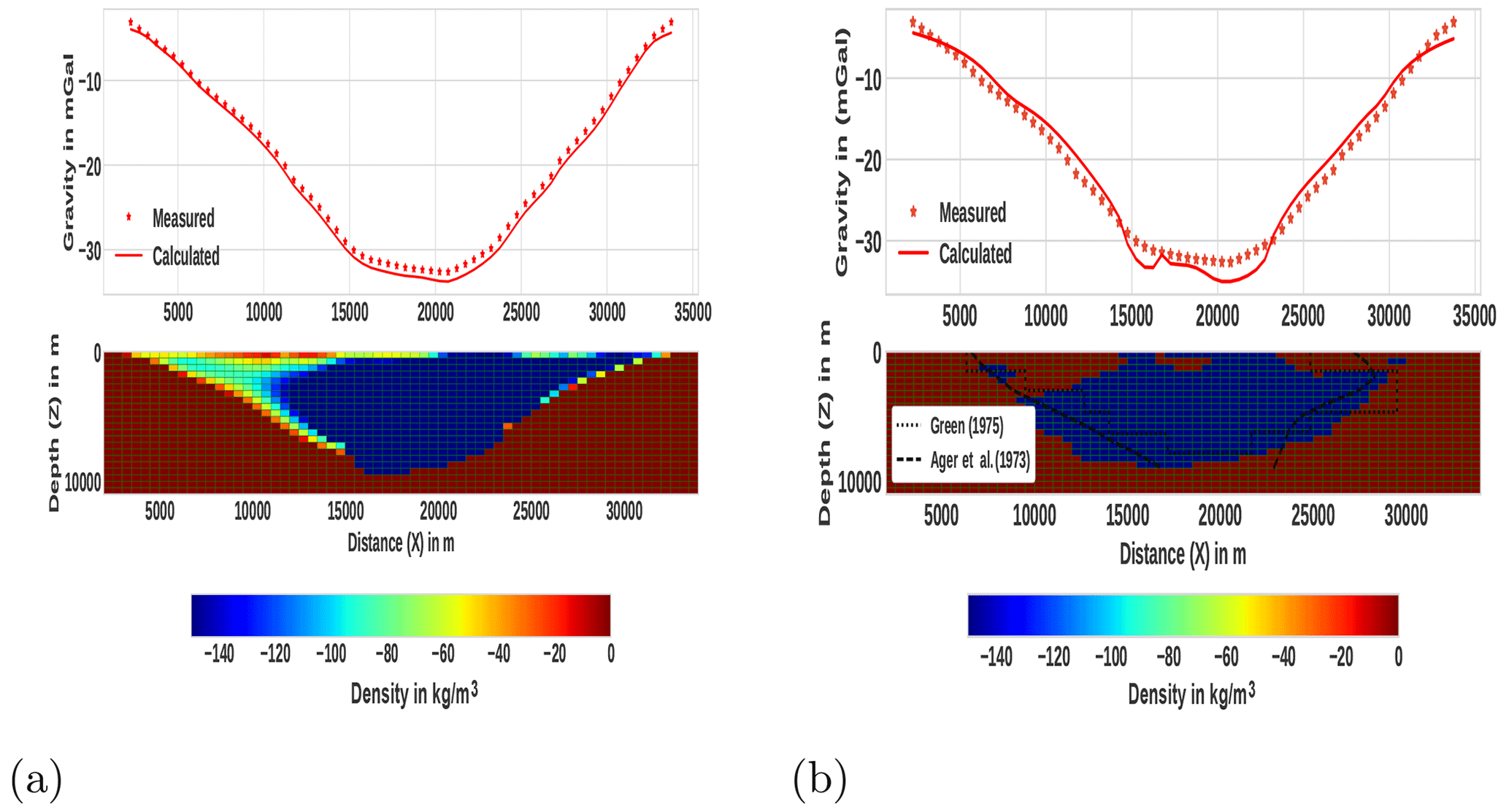
Figure 12 The observed gravity anomaly over Guichon Creek batholith in south-central British Columbia (after Green, 1975) and its inversion results. Digitized data (star marks) with calculated data (solid line) are shown on the top panels of each subfigure. The corresponding recovered density contrast models are shown on the bottom. For comparison, the results obtained by Ager et al. (1973), which were obtained from drilling, and from Green (1975) are also presented. (a) Using the conventional minimum norm (L₂-norm) smooth stabilizer. (b) Using the presented method.

For the inversion, the source volume beneath the anomaly was divided into 64 × 22 square lattices, with the dimensions of each cell being 0.5 km in both the x and z directions. Based on the a priori information from Ager (1972), density values were constrained between the limits ${\mathit{\rho }}_{\min }=-\mathrm{150}$ kg m⁻³ and ρ_max=0.001 kg m⁻³. We start the inversion with a homogeneous initial model in which every block has the same zero density and an initial ℓ_o value of 0.48. The inversion was terminated after the ninth iteration because the stopping criteria were fulfilled. The resulting model is presented in Fig. 12b. For comparison, the results obtained by Ager et al. (1973) and by Green (1975) are also included in Fig. 12b. In addition, using the same inversion parameters, we have performed L₂-norm-regularized inversion, and the obtained result is shown in Fig. 12a. The shape, real extent of the anomaly and depth to bottom from the developed method are very close to the true geological feature (Ager et al., 1973), which was obtained from drilling. That means the implementation of the presented method resulted in a better solution compared to Green (1975) and the conventional L₂-norm inversion. Note that this reasonable result is obtained by using only the density contrast limits as a priori information.

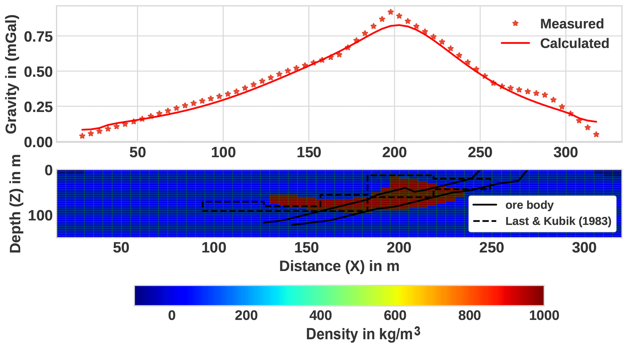
Figure 13 An observed gravity anomaly over the Woodlawn ore body, New South Wales (after Last and Kubik, 1983), and its inversion result. The digitized data (star marks) are shown together with calculated data (solid line) on the top panel. The corresponding recovered density contrast model after the 11th iteration is shown on the bottom panel, and the ore body proved by drilling is shown with the solid line. The recovered body density contrast is represented by the color scale bar.

The second test on measured gravity data is carried out using the published data by Last and Kubik (1983) over the Woodlawn massive sulfide ore body, New South Wales, Australia. The residual anomaly of the area, consisting of 61 data measurements, sampled every 5 m, is digitized from Last and Kubik (1983). The details about the data measurement and the geology of the area are discussed in Whiteley (1981). The model subsurface was divided into 61 by 30 blocks with a dimension of 5 m in both the x and z directions. Inverse modeling was performed with bounding constraints ${\mathit{\rho }}_{\min }=-\mathrm{600}$ and ρ_max=1000 kg m⁻³. The initial given value for ℓ_o was 0.6. The final solution was obtained after the 11th iteration. The reconstructed model, including the final model of Last and Kubik (1983), is shown in Fig. 13. The cross-section of the ore body verified by drilling (Whiteley, 1981) is also shown in the figure.

The recovered model is approximately coincident with the shape, depth of burial and density of the known ore body. Areas of misfits in the current and previous works are believed to be caused by the termination of the original data at both ends before having reached the background level. Thus, this can be additional evidence that the presented method can be successfully applied to real data.

5 Conclusions

We have presented an alternative gravity inversion method that can produce compact and sharp images by using the L₀-norm-stabilizing functional that helps to model geological features with non-smooth, blocky geologic bodies. Physical parameter inequality constraints and depth weighting are integrated into the procedure. The method also incorporates an auto-adaptive regularization technique, which automatically determines a suitable regularization parameter at every iteration, and an error-weighting function that helps to improve both the stability and convergence of the method. One of the strongest sides of the proposed auto-adaptive regularization and error-weighting matrix is that they are not dependent on a priori knowledge of the noise level. Because of that, the method can yield reasonable results even when the noise level of the data is not known properly. We implemented a combined stopping criteria and illustrated its effectiveness to terminate the iterative inversion process after an optimal number of steps. To illustrate the efficiency and the capacity of the proposed procedure, numerous synthetic tests were done. From these, four synthetic examples were presented. According to the results from these synthetic examples, the method can be applied for multi-source localized bodies located at different depths and having different geometries with sharp features. Furthermore, the method proved to be efficient in resolving causative bodies both vertically and laterally and produced compact and sharp images. The obtained results also indicate that the method behaves well with different noise levels embedded in the data and still retains its stability. This can confirm the robustness and stability of the developed inversion method for different noise levels. The method was also tested on measured gravity data. We obtained geologically acceptable models, and the results showed that our approach is effective and reliable. From a computational point of view, the method is efficient and can be easily run on a personal computer in just a few seconds. In conclusion, the developed method is advantageous in that it is stable, efficient and resolves sharp subsurface futures with acceptable resolving capacity. In geophysical exploration, gravity data are more often used to image complex 3D structures of the subsurface; hence further development of the method to 3D is crucial. Accordingly, future work will deal with the extension of the presented method to a 3D gravity inversion algorithm.