A new seismicity catalogue of the eastern Alps using the temporary Swath-D network

We present a new, consistently processed seismicity catalogue for the eastern and southern Alps based on the temporary dense Swath-D monitoring network. The final catalogue contains 6053 earthquakes for the time period 2017–2019 and has a magnitude of completeness of −1.0 M_L. The smallest detected and located events have a magnitude of −1.7 M_L. Aimed at the low to moderate seismicity in the study region, we have developed a multi-stage, mostly automatic workflow that combines a priori information from local catalogues and waveform-based event detection, subsequent efficient GPU-based (GPU: graphics processing unit) event search by template matching, P and S arrival time pick refinement, and location in a regional 3-D velocity model.

The resulting seismicity distribution generally confirms the previously identified main seismically active domains but provides increased resolution of the fault activity at depth. In particular, the high number of small events additionally detected by the template search contributes to a denser catalogue and provides an important basis for future geological and tectonic studies in this complex part of the Alpine orogen.

1 Introduction

The Alps form the largest and highest mountain range in Europe and are the result of the collision between the European plate and the Adriatic microplate. The influence of crustal indentation on the Alpine orogen has been revealed by geological–geophysical transects and passive seismic experiments across the western, central, and eastern Alps, such as ECORS-CROP (Nicolas et al., 1990), NFP20 (Pfiffner et al., 1990), TRANSALP (TRANSALP Working Group et al., 2002; Schmid et al., 2004), EASI (Hetényi et al., 2018), and CIFALPS (Malusà et al., 2021). These and teleseismic, local earthquake, and ambient-noise tomography studies have also revealed the complexity of the crustal and upper-mantle structure (e.g. Piromallo and Morelli, 2003; Lippitsch et al., 2003; Bleibinhaus and Gebrande, 2006; Diehl et al., 2009; Zhao et al., 2015; Hua et al., 2017; Kissling and Schlunegger, 2018; Kästle et al., 2018, 2020; Lu et al., 2020; Qorbani et al., 2020; Nouibat et al., 2021; Paffrath et al., 2021; Jozi Najafabadi et al., 2022; Paul, 2022). Specifically in the eastern and southern Alps, however, key questions regarding the deeper structure such as the possible existence and location of a slab polarity remain controversial (e.g. Lippitsch et al., 2003; Kummerow et al., 2004; Handy et al., 2010; Mitterbauer et al., 2011; Kästle et al., 2020; Mroczek et al., 2023).

Another approach to illuminate the crustal structure and tectonic processes is the analysis of earthquake activity. The overall diffuse shallow seismicity in the Alps was investigated by various studies, ranging from regional to local scales (e.g. Nicolas et al., 1998; Bethoux et al., 1998; Reinecker and Lenhardt, 1999; Chiarabba et al., 2005; Ustaszewski and Pfiffner, 2008; Anselmi et al., 2011; Bressan et al., 2012; Viganò et al., 2015; Reiter et al., 2018; Beaucé et al., 2019; Jozi Najafabadi et al., 2021; Saraò et al., 2021).

Until recently, homogeneous monitoring of the Alpine seismicity was impeded by an irregular configuration of permanent seismic stations and non-uniform procedures of national seismological agencies. The regional-scale AlpArray initiative (Hetényi et al., 2018) finally enabled a new coherent analysis of the earthquakes in the greater Alpine region, producing the AlpArray seismicity catalogue with a magnitude of completeness of M_c=2.4M_LV (Bagagli et al., 2022).

Embedded into AlpArray, the additional denser Swath-D network, comprising 151 uniformly spaced stations in the eastern and southern Alps, was operated for approximately 2 years in the time period 2017–2019 (Heit et al., 2021, and Fig. 1). In this study, we exploit the new data contributed by the Swath-D network and the data from adjacent stations to build a consistently processed, more detailed earthquake catalogue focusing on the eastern and southern Alps and provide the basis for a subsequent in-depth analysis of seismicity and the related fault structures.

The Swath-D region of the Alps is characterised by relatively low to moderate seismicity (e.g. Slejko et al., 1998; Reiter et al., 2018). Nonetheless, it is routinely monitored by different agencies which already provide local earthquake catalogues of high quality (Istituto Nazionale di Oceanografia e di Geofisica Sperimentale (OGS), 2016; INGV Seismological Data Centre, 2006; Swiss Seismological Service (SED) at ETH Zurich, 1983). We have therefore developed an event detection and location workflow that both integrates the already existing information and exploits the newly available data from the Swath-D monitoring network. We first build a preliminary earthquake catalogue based on the local event catalogues which we complement with an energy-based detection using the entire continuous waveform archive of the Swath-D network and waveforms from neighbouring stations in the same time period. We then search for smaller, hitherto undetected events with a template matching technique; i.e. we scan the continuous waveform data for similarity to waveforms from the preliminary event catalogue. A number of applications have demonstrated the effectiveness of this approach to increase the number of low-magnitude earthquake detections (e.g. Gibbons and Ringdal, 2006; Skoumal et al., 2015; Vuan et al., 2018; Ross et al., 2019; Beaucé et al., 2019). In order to cope with the large data volume caused by the high number of seismic stations (198, including Swath-D and adjacent stations from AlpArray and local monitoring networks), as well as the relatively long registration period (24 months) and high sampling rate (100 Hz) of the Swath-D network, we developed an efficient template matching code. The calculation of the cross-correlation functions, which we use as the measure of waveform similarity, makes use of the graphics processing unit (GPU) to accelerate the processing. For each event cluster defined by the previous template search, we identify a reference event and manually pick P and S arrival times. We then automatically associate new picks for all cluster events by using relative arrival times determined from a combination of the cross-correlation function and the short-term average to long-term average ratio (STA $/$ LTA). The P and S arrival times in the extended set are then inverted for event location and origin time in a local 3-D velocity model. Since the eastern Alps are densely populated and industrialised, anthropogenic signals are recorded alongside seismic events (Peruzza et al., 2015). We identify these anthropogenic signals based on their typical temporal signatures and confirm their origins using satellite images. Finally, we describe the characteristics of the seismicity distribution in detail.

2 Data

This study focuses on seismicity which was recorded by the Swath-D network (ZS) (Heit et al., 2021). The Swath-D network complemented and densified the larger-scale AlpArray backbone network (Hetényi et al., 2018) in the eastern Alps. It formed a temporary array of broadband seismic stations and recorded during the time period from late 2017 to late 2019.

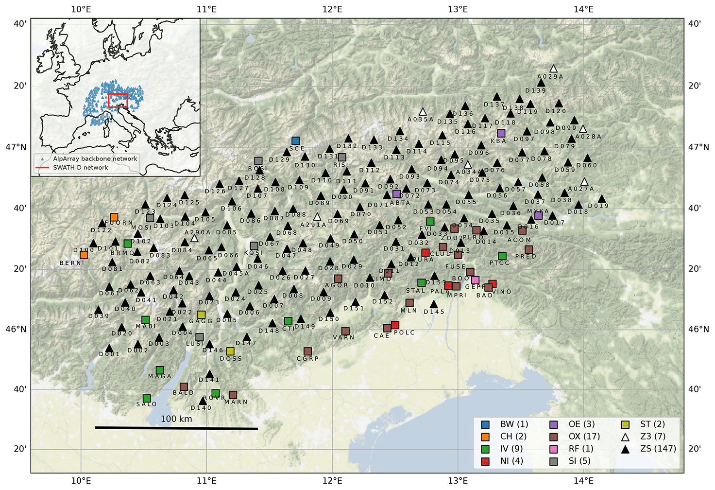
Figure 1 Map of the study area in the eastern Alps showing the distribution of the stations used. Triangles and squares represent temporary and permanent stations, respectively, and the colours refer to the networks. Network ZS is the Swath-D network (Heit et al., 2021), and Z3 represents the stations from the AlpArray backbone network (Hetényi et al., 2018). BW is managed by the Department Of Earth And Environmental Sciences, Geophysical Observatory, University Of München (2001), network CH is managed by the Swiss Seismological Service (SED) at ETH Zurich (1983), networks IV, NI (in collaboration with the OGS), RF, SI, and ST are managed by the INGV Seismological Data Centre (2006), network OE is managed by the ZAMG-Zentralanstalt Für Meterologie Und Geodynamik (1987), and network OX is managed by Istituto Nazionale di Oceanografia e di Geofisica Sperimentale (OGS) (2016) in collaboration with the INGV. Map background by http://stamen.com/ (last access: 2 August 2023; Stamen Design) under http://creativecommons.org/licenses/by/3.0 (last access: 2 August 2023; CC BY 3.0).

Swath-D had a total of 151 stations initially, with an aperture of around 15 km, establishing unprecedented station coverage for the region. The majority of the stations in the initial network (147 stations) were deployed in the fall of 2017. Four stations (D030, D142–D144) were deployed in the summer of 2018. By the end of 2018, 10 additional stations (D154–D163) were added, extending the network to the east (Schlömer et al., 2022). Data from the stations deployed after 2017 were not used in this study to ensure a more stable network geometry and hence resolution. For completeness, all publicly available broadband stations within approximately 50 km of the Swath-D network that were active in that period were also included in this study. These comprise stations from OGS (Istituto Nazionale di Oceanografia e di Geofisica Sperimentale (OGS), 2016), LMU (Department Of Earth And Environmental Sciences, Geophysical Observatory, University Of München, 2001), SED (Swiss Seismological Service (SED) at ETH Zurich, 1983), INGV (INGV Seismological Data Centre, 2006), and ZAMG (ZAMG-Zentralanstalt Für Meterologie Und Geodynamik, 1987), as well as stations from the AlpArray backbone network (Hetényi et al., 2018). Figure 1 shows a map of the distribution of stations in the Swath-D network, as well as of all other stations used in this study.

3 Method

In the following, we describe our event detection and location workflow in more detail. It is sketched in Fig. 2 and consists of three main components: (1) compilation of a preliminary event list and clustering, (2) GPU-based template matching for detecting small events, and (3) cluster-based arrival time assignment and pick refinement.

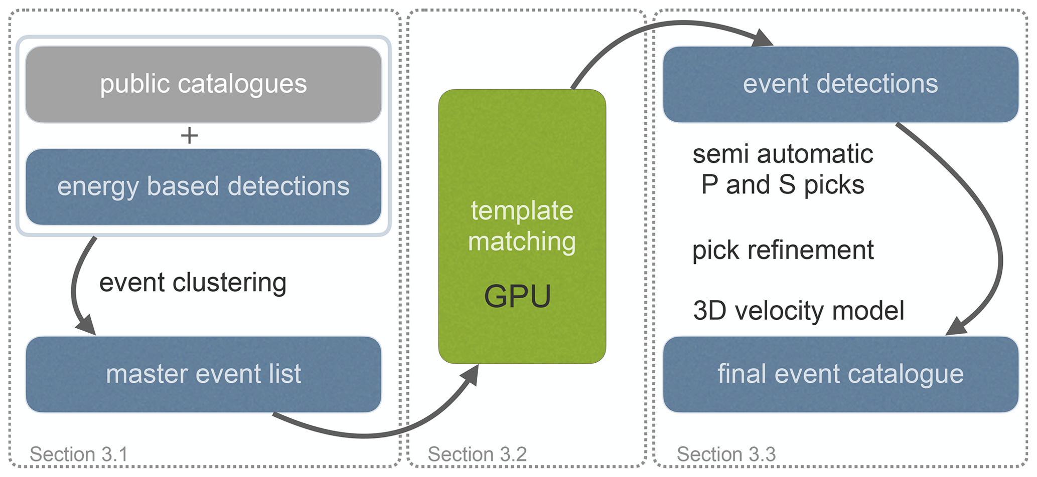
Figure 2 Schematic overview of the workflow and methods applied in this study. The dotted outlines refer to the three main parts of the Method section where the steps are explained.

3.1 Compilation of a preliminary event list and clustering

A basic requirement for efficient event search by template matching is a robust list of pre-selected events whose waveforms define the templates. Several agencies provide earthquake catalogues that cover at least part of the study region in the eastern Alps (Istituto Nazionale di Oceanografia e di Geofisica Sperimentale (OGS), 2016; INGV Seismological Data Centre, 2006; ZAMG-Zentralanstalt Für Meterologie Und Geodynamik, 1987; Swiss Seismological Service (SED) at ETH Zurich, 1983). We merge these catalogues and remove multiple entries by imposing a minimum interevent time of 15 s or a minimum distance of 50 km. Only events with a maximum distance of 50 km to the nearest station within the Swath-D network are considered. We found 3455 unique events that meet these criteria.

Additionally, we apply the energy-based detection algorithm Lassie (Heimann et al., 2017) to the entire continuous waveform database of the Swath-D experiment in order to exploit the increased station density compared to the permanent networks in the area. This also compensates for the heterogeneous sensitivity of the available catalogues in the study region and identifies previously undetected earthquakes, particularly in the central part of Swath-D. The method involves stacking the energy functions of different stations assuming a predefined grid of potential hypocentral locations and origin times. This allows detecting the source of coherent seismic signals, the origin time of which corresponds to the temporal coordinate of the maximum, and the spatial coordinates of the maximum can be used to infer its approximate location. The extent of the search region is 360 km by 240 km in the longitudinal and latitudinal directions with 5 km node spacing. The source depth is fixed to 15 km. By default, data from all stations contribute to the characteristic function for each grid node. This decreases the sensitivity for small events because their signals will be registered only by stations close to the event epicentre, and by including too many stations, these signals will be diluted. We therefore implemented a new class for the weighting of the individual stations so that a maximum number of contributing stations around each node can be fixed. Of the 3511 events that are detected using Lassie, the majority are found to exist in at least one of the public catalogues. From the remaining detections, 592 events can be located. A total of 306 of these remaining events are classified as anthropogenic noise (see Sect. 4 for details on the classification), leaving 286 potential new earthquake detections. More details, including an example of an event detection using this method, can be found in Sect. S1.1 in the Supplement.

The catalogue earthquakes and the additionally detected events are then combined, and waveforms are cross-correlated with group events into clusters. Two events are connected if the event waveforms are similar (i.e. the median of the three highest maximum cross-correlation coefficients exceeds 0.7). The similarity is measured for a 10 s time window that includes both the P-phase and S-phase arrival on the vertical channel. Within each cluster, the event that has the highest number of connections is selected as the master event.

In the specific case of the Swath-D data, it turns out that the signal to noise ratio is poor for many low-magnitude events, and in some cases coherent noise leads to erroneously merging groups of events into a common cluster without actually being similar events. To solve this problem, we apply the Louvain method (Blondel et al., 2008) to find the partition of the cluster into sub-clusters (also communities) that maximises the modularity. This is a measure of the number of connections within a sub-cluster compared to the connections to the rest of the network (Newman, 2006). If the modularity is below 0.5, we consider the cluster well connected as a whole and leave it as it is. If the modularity is 0.5 or higher, we accept the partition and split the cluster into sub-clusters, each with an individual master event that has the highest number of connections within the sub-cluster. This results in a list of 2036 events to be used as master events for template matching.

3.2 GPU-based template matching for detecting low-magnitude events

Preprocessing. Template matching in seismology is usually performed by using either single phases (e.g. Ross et al., 2019) or the entire event waveforms as templates (e.g. Beaucé et al., 2019). Using the P and S phases separately has the advantage that the S–P travel time is not constrained, and therefore events can be detected further away from the master events. On the other hand, using shorter template waveforms massively increases the number of false triggers for prevalent weak signals, as is the case for the Swath-D network. We therefore choose to use the entire event waveform.

For each of the 2036 master events, we extract template waveforms of 10 s length to ensure that the P and S phase are both included for local events. The template window starts approximately 2 s before the P-wave onset and is calculated by assuming a straight ray path and constant P-wave velocity. All waveforms are downsampled to 50 Hz to decrease computation time. We apply a bandpass filter between 2 and 8 Hz. This suppresses high-frequency noise recorded by some of the temporary Swath-D stations and allows slightly more variation in the event waveforms of the detected events compared to using a wider range of frequencies. Note that we do use a wider frequency band for picking to improve the accuracy (see Sect. 3.3). For each master event, template waveforms are extracted on the vertical component of the 15 stations closest to the event hypocentre. Additionally, an STA $/$ LTA trigger is applied to the waveforms to make sure that a transient signal occurs within the template window. The STA window (0.1 s) should have at least 5 times the amount of energy as the LTA window (1 s). Template waveforms that do not meet this criterion are dismissed. This results in 28 207 template waveforms, averaging 14 template waveforms per event.

Template matching. For each template waveform we then search for similar events. This approach is computationally demanding, in particular for distributed seismic networks, because for each component it involves cross-correlation with the corresponding continuous waveform data. To make it feasible for the Swath-D station configuration, we decided to implement our own GPU-based template matching code. We achieve a major performance increase by reformulating the cross-correlation as a matrix multiplication in the frequency domain using CuPy, a Python library for GPU-accelerated computing (Okuta et al., 2017). Additionally, the number of I/O operations is reduced to a minimum by loading each continuous data trace only once. Using a single Nvidia GV100 graphics processing unit (GPU) with 8192 cores, the processing time was cut by a factor of 100 compared to a serial approach on our local machine.

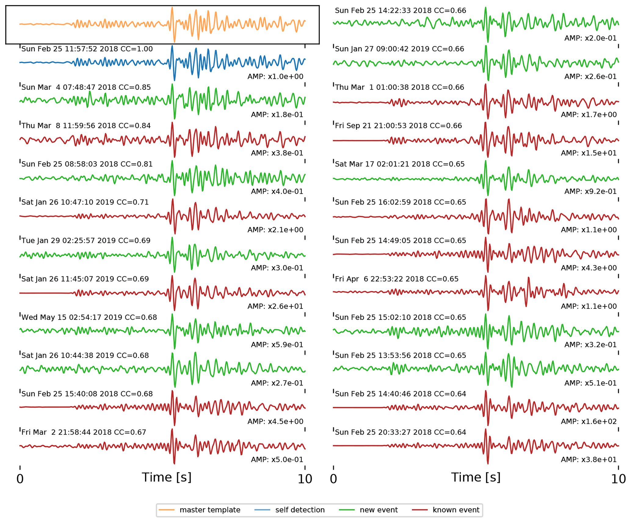
Figure 3 Example of template matching results for a single template on one station. The upper left trace in orange is the template waveform. The other traces are detections sorted by the cross-correlation coefficients starting with the self-detection (of the template trace within the continuous data) in blue. The other detections are coloured red if they can be associated with an event in any of the public catalogues or green if they cannot be associated with any known event. The maximum amplitude of each signal is indicated as a factor of the maximum amplitude of the template waveform. It can be observed that all signals with amplitude equal to or larger than the template signal appear in one of the public catalogues, whereas all newly detected signals have amplitudes lower than the template.

A peak search algorithm sorts all peaks in the cross-correlation function and dismisses any peak that is within 10 s of a larger peak. A match is triggered when the cross-correlation coefficient, CC, exceeds 0.5 on three different stations within a 5 s time window using templates that were extracted for the same master event. The 5 s time window corresponds to the estimated origin time of the detections. This estimate is obtained by adding the cross-correlation shift, the start time of the data trace, and the origin time of the master event and subtracting the start time of the template window.

This method yields 15 155 event detections including self-detections of the master events, a 7-fold increase with respect to the number of master events, or a 4-fold increase with respect to the combined public catalogues and energy-based detections. At this stage, the detections may include anthropogenic signals such as quarry blasts, which were partially omitted from the public earthquake catalogues.

3.3 Cluster-based semi-automatic P and S arrival time assignment and pick refinement

Through template matching, the detected events are implicitly clustered into event families. These contain all events that were detected using templates from the same master event. The events within one family have a similar location because they both have similar waveforms for at least three stations as well as similar relative travel times for these stations. This means that we know roughly when to expect phase arrivals for the events within one family, as long as we have picks for at least one event. In this section, we describe our procedure for picking the P and S arrival times of all detected events, starting with one hand-picked master event for each event family.

Firstly, we hand-pick P- and S-phase onsets on the 10 closest stations for all master events. This gives us 23 426 picks, an average of 11 picks per event. These picks are referred to as master picks in the rest of this section. For all other detected events within the cluster, we estimate the phase arrivals by adding the travel times from the master event to the origin time estimate. We then define a window of 3 s around this first guess that we refer to as the predicted phase window. The waveforms are preprocessed phase dependently. A 1–20 Hz bandpass filter is applied for P phases, and a 1–12 Hz bandpass filter is used for the S phases. These frequency bands are wider than the one used for template matching (see Sect. 3.2) to improve the accuracy of the picks. Secondly, the trigger function is calculated for the predicted phase window. The first part of the trigger function is a normalised short-term average to long-term average ratio (STA $/$ LTA). We used an STA length of 0.2 s and an LTA length of 0.6 s for P phases and 0.8 s for S phases, respectively. The STA window runs ahead of the current sample, whereas the LTA window is behind the current sample, as by the definition of Earle and Shearer (1994). In this way, the maximum value aligns with the phase onset. For the second part of the trigger function, the predicted phase window is cross-correlated with the corresponding master pick. Time windows of 0.5 and 1.5 s around the master pick are used for P and S phases, respectively, both starting 0.2 s before the actual pick. These two parts are combined by pointwise multiplication to form a new trigger function. The final pick time is set to the maximum of this trigger function, with the possibility of setting individual thresholds for the cross-correlation function and the STA $/$ LTA. Approximately 65 000 picks are made using this method. An example is shown in Fig. S2 in the Supplement.

Because our trigger function requires a hand-pick, it is limited to the channels that were hand-picked on the master event. Due to changes in the station availability over time, a slightly different set of stations might be available for certain events. We use a classic STA $/$ LTA trigger to pick phases on these additional stations. The STA $/$ LTA trigger is applied after a first relocation iteration so that phase windows can be estimated more accurately, yielding an additional 30 000 picks.

This combined arrival time picking procedure provides roughly 95 000 new P and S picks for a total of about 9 000 events, originally starting with a small subset of about 2000 master events. These numbers will be slightly reduced during the location procedure, where picks that produce anomalous residuals are dismissed and a minimum number of picks per event is required.

Since we have used a mixture of three different picking techniques, we finally adopt a method proposed by Shearer (1997) to homogenise our set of picks. The method combines, for each channel and phase, cross-correlation-based differential travel times dt_ij and absolute time picks t_i within each template family and solves for an improved set of adjusted time picks T_i. We apply this technique iteratively and obtain a more consistent final set of P and S arrival time picks. For more details on the method and for data examples, we refer to Sect. S1.3.

The determined P and S arrival times are then inverted for event locations, as described in the following section. We use the probabilistic NonLinLoc software (Lomax et al., 2000) and a recent 3-D velocity model for both P and S phases based on local seismic tomography by Jozi Najafabadi et al. (2022), which fully covers the study region.

4 Results and discussion: seismicity of the eastern Alps

On the basis of our preliminary event list (2036 events; see Sect. 3.1 for details), we detected 15 155 events using template matching. Each detection consists of a minimum of three independent, simultaneous measurements on three different stations as explained in Sect. 3.2. By applying our specific semi-automatic picking workflow (Sect. 3.3), we are able to successfully pick and relocate 7756 events (Fig. 4).

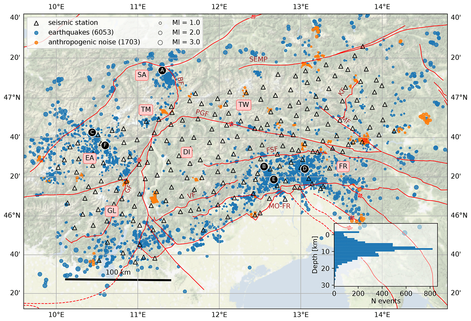
Figure 4 Map of the distribution of events found in this study classified as earthquakes (blue dots) and anthropogenic events (orange dots). Major faults from Schmid et al. (2004) are indicated with red lines (available at http://www.spp-mountainbuilding.de/data/tectonic_maps_4dmb_03-2022.zip, last access: 18 April 2022). The abbreviations are as follows. SEMP: Salzach–Enns–Mariazell–Puchberg fault, PGF: Pustertal–Gailtal fault, BF: Brenner fault, GF: Giudicarie fault, VF: Valsugana fault, KF: Katschberg fault, MF: Mölltal fault, FSF: Fella–Sava fault, MO-FR: Montello–Friuli thrust belt. Tectonic units are named as in Reiter et al. (2018), TW: Tauern window, DI: Dolomite Indenter, FR: Friuli, GL: Giudicarie–Lessini region, EA: Engadine Alps, TM: Texel group and Meran–Passeier area, SA: Stubai Alps. Symbols A–F mark the locations of earthquake sequences indicated in Fig. 7. Map background by http://stamen.com/ (Stamen Design) under http://creativecommons.org/licenses/by/3.0 (CC BY 3.0).

For an event to be located, we require a minimum number of six picks, with at least one station that has both a P and S pick in order to better constrain event depth. The maximum allowed weighted residual root mean square (rms) after inverting for the hypocentre is 250 ms, where the residuals are subjected to a station correction term based on the median residual within the template family. Our final catalogue is based on a total of 93 576 picks, averaging 12 picks per event.

4.1 Event classification

To first differentiate between natural seismicity and anthropogenic events, we analyse the temporal patterns of each individual template family. Natural seismicity is expected to be randomly distributed in time, whereas anthropogenic noise usually occurs during daytime, either within a limited time window or at fixed times. Also, the number of anthropogenic noise events is much higher during weekdays compared to weekends. Histograms of these temporal features are inspected manually for all template families containing three or more events. In the case that an anthropogenic signature is suspected, we consult satellite imagery to look for quarries or construction sites. This leads to the identification of 1659 events related to two dozen anthropogenic noise sources. In Fig. 4, their distribution is indicated by orange symbols. The distinct temporal patterns of both classes are shown in Fig. 5. The anthropogenic signals occur exclusively during daytime, with clear peaks at 12:00 and 17:00 (local time) and only on working days. In addition, this figure reveals a slightly increased sensitivity to natural seismic events at night and on weekends. These are the times when noise levels are usually lower. An example of a template family containing anthropogenic signals and their identification using the temporal signatures and satellite imagery is shown in Fig. S5.

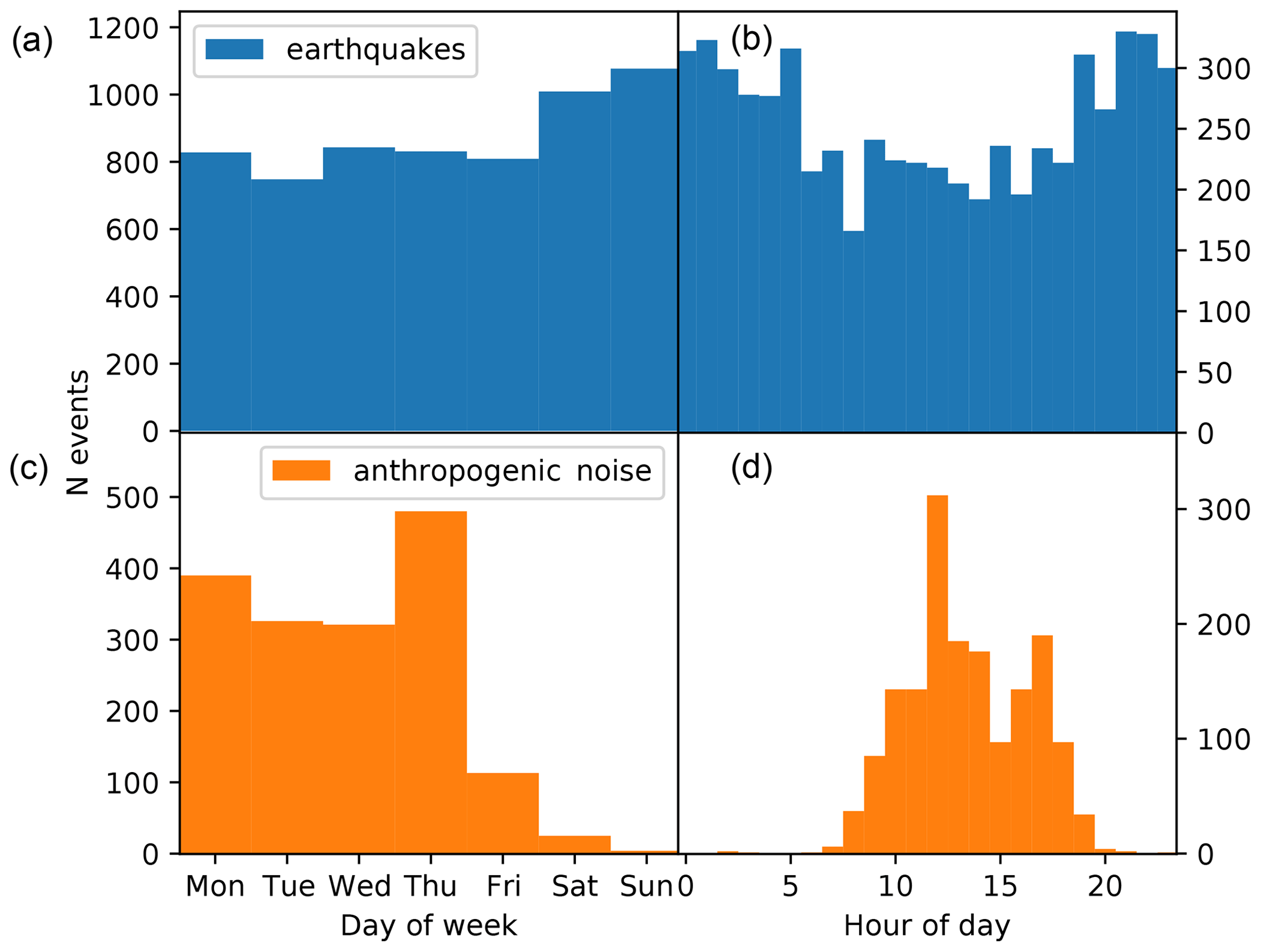
Figure 5 Histograms of the weekday (a, c) and hour of the day (c, d) for the events classified as earthquakes (a, b) and anthropogenic noise (c, d).

4.2 Magnitude distribution

After removing the anthropogenic signals from our catalogue, 6053 events remain which we classify as tectonic earthquakes (blue circles in Fig. 4). Local magnitudes (Richter, 1935) are calculated completely independent of the public catalogues. Their frequency–magnitude distribution (FMD) is shown in Fig. 6. As expected, template matching particularly increases the number of low-magnitude events. The smallest located earthquakes have a magnitude of about −1.7 M_L, and the magnitude of completeness M_c is −1.0 M_L based on the maximum curvature of the FMD (Wiemer and Wyss, 2000). The corresponding b value (Gutenberg and Richter, 1944) is 0.70 and slightly higher than the value obtained for the limited group of master events (b=0.68, with $M_{\mathrm{c}}=-\mathrm{0.2}{M}_{\mathrm{L}}$). We refer to Sect. S1.5 for a detailed description of the magnitude calculation method, as well as an estimation of the moment magnitudes M_w in Fig. S6.

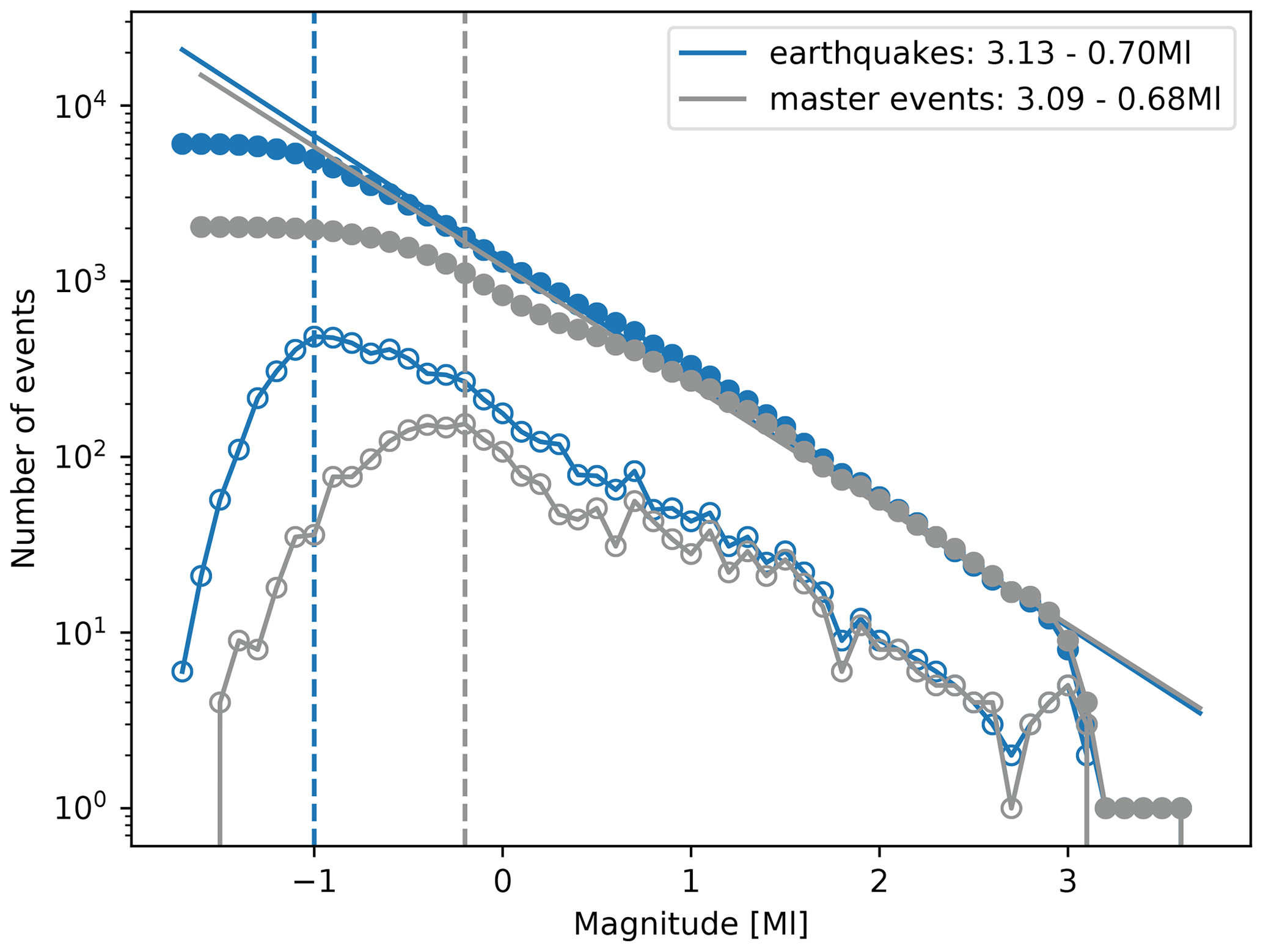
Figure 6 Frequency–magnitude distribution of the master events (grey) and the final earthquake catalogue (blue). We obtain the values a=3.13 and b=0.70 for the Gutenberg–Richter relation (Gutenberg and Richter, 1944) using a least-squares fit. The completeness magnitude M_c was estimated at −1.0 M_L based on the maximum curvature of the FMD (Wiemer and Wyss, 2000).

4.3 Temporal patterns in seismicity

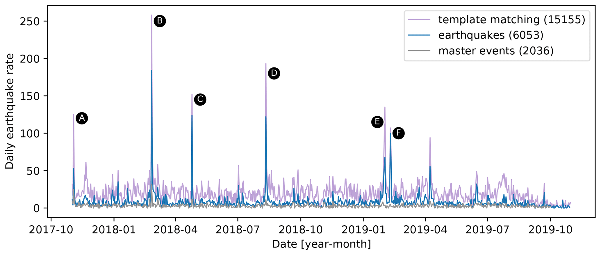
Throughout the recording period, we observe a fairly constant background seismicity rate of about 20 events per day (Fig. 7). This mode alternates with short episodes of intense seismic activity, which become particularly evident through the template matching. There are six occurrences where the daily detection rate exceeds 100 events per day. These sequences and their locations are marked by symbols A–F in Figs. 4 and 7. The first is on 3 November 2017 (A). This corresponds to a seismicity cluster in the Stubai Alps, south of the city of Innsbruck. The largest earthquake in this sequence has a magnitude of 3.02 M_L. The second and largest peak is on 25 February 2018 (B). This cluster is located north of the village of Cimolais, on the Friuli–Veneto border. It contains a magnitude 3.05 M_L event and a magnitude 2.88 M_L event. The third is on 25 April 2018 (C), with a maximum magnitude of 2.13 M_L in the Münstertal on the Swiss–Italian border. The fourth is on 11 August 2018 (D). This sequence is located south of the town of Tolmezzo, and it contains one event with a magnitude of 2.91 M_L. The fifth is on 1 February 2019 (E). This sequence in the Friuli region west of the village of Chievolis has a maximum magnitude of 0.35 M_L. The sixth and last is on 9 February 2019 (F) in the Suldental on the Swiss–Italian border. This sequence has a maximum magnitude of 1.24 M_L. As an example, the relocated events of this cluster are shown in Fig. S12.

Figure 7 Daily earthquake rate in the initial input catalogue (grey), the template matching detections (purple), and the final relocated catalogue (blue). Sequences that exceed a daily rate of 100 events are indicated with symbols A–F in Fig. 4.

4.4 Spatial distribution of seismicity

The epicentral seismicity distribution from this study, which is restricted to the recording period of the Swath-D network in the years 2017–2019 (Figs. 4 and 8), largely corresponds to the long-term behaviour of M_L > 2.0 earthquakes obtained in earlier studies (Slejko et al., 1998; Reiter et al., 2018). Seismicity is mostly shallow, with 98 % of the seismic events occurring within the upper 20 km of the crust (see the depth histogram in Fig. 4). This is consistent with previous studies in the eastern Alps (Reinecker and Lenhardt, 1999; Viganò et al., 2015; Reiter et al., 2018; Jozi Najafabadi et al., 2021). The major parts of the event hypocentres (75 %) are in the band of 5 to 15 km depth, with pronounced concentrations of earthquakes between 8 and 12 km depth.

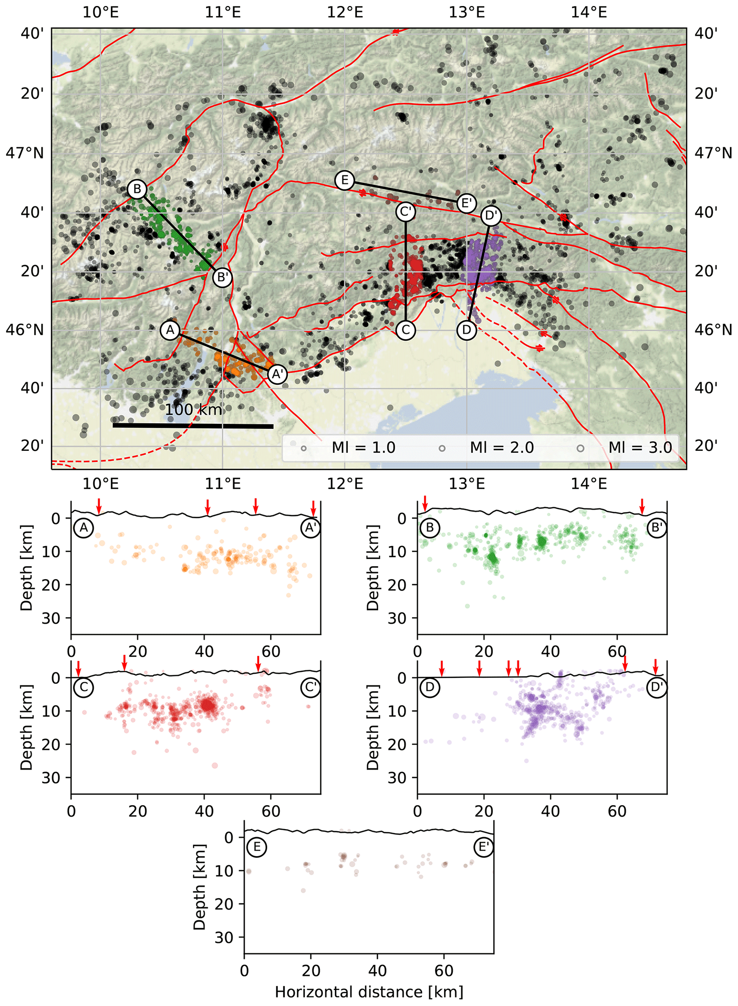
Figure 8 Five exemplary cross-sections of the seismicity in the area. The horizontal axes of the sections are indicated on the map in the upper panel. The colours are solely to indicate which events are used in the sections. Vertical red arrows mark the intersections of the cross-section with fault traces shown on the map. Topography profiles were extracted from the ETOPO 2022 global relief model (NOAA National Centers for Environmental Information, 2022). Map background by http://stamen.com/ (Stamen Design) under http://creativecommons.org/licenses/by/3.0 (CC BY 3.0).

The spatial patterns reflect the NNW convergence of the Adriatic microplate and the European plate, with active seismic deformation occurring mostly in the thrust-and-fold belt in the south-eastern Alps, which separates the indenter from the undeformed part of Adria (Castellarin et al., 2006; Cheloni et al., 2014; Serpelloni et al., 2016; Reiter et al., 2018; Petersen et al., 2021). Here, seismicity is most prevalent in the Montello–Friuli thrust belt in the south-eastern corner of the study area (Romano et al., 2019; Bragato et al., 2021). This is by far the most seismically active area during the recording time of the Swath-D network. This area was witness to the largest instrumental earthquake in northern Italy, the devastating 6.4 M_L Friuli earthquake (e.g. Slejko, 2018; Aoudia et al., 2000). The density of magnitude M_L > 2 events in this area is much higher compared to the rest of the study area. To the south, the seismic activity spills over into the Po basin, following the pattern of known historical seismicity, whereas to the north, most of the seismic activity is cut off sharply by the Fella–Sava and Valsugana faults. Seismicity to the north of these faults, within the north-western part of the Dolomite indenter, is much sparser. Recent crustal tomography studies show that this area is characterised by a positive anomaly of Rayleigh-wave phase velocities at seismogenic depths, indicating a denser and possibly more rigid upper-crustal block (Sadeghi-Bagherabadi et al., 2021; Kästle et al., 2021).

Nonetheless, we are able to relocate roughly 100 events, particularly benefiting here from the improved resolution in the central part of the Swath-D network compared to the permanent station configuration. These events are generally below magnitude 1 M_L, except for two events close to the Fella–Sava fault. The seismicity rate increases slightly within the Tauern window further northwards, starting on the Pustertal–Gailtal fault, a segment of the dextral Periadriatic fault. Our catalogue contains roughly 200 events in this area. From modelling GPS velocities, the Pustertal–Gailtal fault is assumed to accommodate part of the NW indention (Caporali et al., 2013). We find earthquakes that align along an almost 100 km long section of the Pustertal–Gailtal fault between about 12.0 and 13.0^∘ E. The strike-parallel depth section in Fig. 8 (profile EE') shows the seismicity here at a fairly constant depth of 5–10 km.

Further to the east, a few events are also observed in a few clusters at variable depths between about 5 and 12 km at the Katschberg fault and the Mölltal fault, extending to its north-western end at about 13.15^∘ E, 47.0^∘ N.

Seismicity within the Tauern window is equally low in magnitude, with few events above magnitude 1 M_L. North of the Salzach–Enns–Mariazell–Puchberg fault, the seismicity rates and the magnitudes increase again, but this area lies outside the Swath-D area and is therefore not within the scope of this paper.

Elevated levels of seismicity are also observed to the west of the indenter boundary, primarily in the Giudicarie–Lessini region and the Engadine Alps, where the seismicity seems to be homogeneously spread without following well-defined patterns. These areas show frequent M_L > 1 events and several magnitude 2 M_L events, especially around the lake Garda area. Further north in the Texel group and Meran–Passeier area, where the magnitude 5.3 M_L event occurred in 2001 (Viganò et al., 2015; Reiter et al., 2018), and in the Stubai Alps, seismicity is more concentrated in a few active clusters. Seismicity rates remain high and magnitudes elevated in the Inntal region on the northernmost detection limit.

We provide two animations in the Supplement that illustrate the 3-D distribution of the Swath-D seismicity catalogue produced here. They visualise the seismicity in continuous north–south and east–west depth slices. Figure 8 shows depth sections along four profiles in different parts of the study region, which provide a more detailed view of the fault activity at depth. They highlight the significant variations of seismic activity from west to east and illuminate the varying complexity of the seismically active structures. In particular, the easternmost profile D in the thrust-and-fold belt in the south-eastern Alps at $\sim \mathrm{13}{}^{\circ }$ E resolves a divergence of dip angles and directions which reflects the intricate interaction of Alpine and Dinaric tectonics (e.g. Bressan et al., 2021).

4.5 Location uncertainty

Location uncertainty can be estimated from the 68 % confidence ellipsoids derived from the probability density functions (PDFs) in NonLinLoc. Histograms of the dimensions of the confidence ellipsoids for all earthquakes are shown in Fig. S9. We observe that the semi-major axes of the ellipsoids are predominantly vertical, meaning that the horizontal coordinates of the seismicity are better resolved than its depth. Mean location errors are of the order of 300 m. Standard deviations of the normally distributed P and S arrival time residuals for all located events are about 0.07 s for P picks and 0.10 s for S picks and are shown in Fig. S8. As an additional appraisal of the location uncertainty, we studied the spatial distribution within event families by calculating the distance of the events relative to the master events. Dependent on the threshold of waveform similarity, the number of events rapidly decreases with interevent distance (Fig. S10). We use a three-station correlation coefficient (CC) defined as the median of the three highest maximum cross-correlation coefficients in a 10 s window containing the event on the vertical channel. The cross-correlation is performed on 15 stations closest to the event. For highly similar event pairs with three-station waveform similarity CC > 0.9, the horizontal event distances are mostly less than 1 km and slightly larger for the vertical distance (1.5 km). We interpret these distances as an upper bound on the location uncertainties by asserting that these events are exactly co-located, in which case the scattering within this subset of events would be attributed to location errors only. In Fig. S11 we analyse the direction of the relative locations with respect to the master events and show that no azimuthal bias can be observed. Figure S12 shows an example of an event cluster with 239 events detected and picked based on 7 master events only. This demonstrates the potential of resolving individual structures using our workflow.

5 Conclusions

We have presented an efficient workflow specifically designed for the detection, phase picking, arrival time pick refinement, and location of small earthquakes and apply it to the dense Swath-D seismic monitoring network in the eastern Alps. Although the region is routinely monitored by several national agencies that provide high-quality seismic event catalogues, our workflow, combined with the integration of the new Swath-D seismological data, increases the number of detected events. The main components of the workflow are a systematic GPU-based template search to detect low-magnitude events and a semi-automatic picking routine to improve the quality and consistency of P- and S-phase picks. This allows, for the first time, a coherent and detailed location of seismicity in the study region using the recent 3-D velocity model by Jozi Najafabadi et al. (2022).

Our catalogue contains 6053 events over a 24-month time period from 2017 to 2019, with magnitudes in the range $-\mathrm{1.7}\le M_{\mathrm{L}}\le \mathrm{3.7}$ and a completeness of −1.0 M_L. The earthquake distribution reproduces the main patterns of seismicity previously found by long-term but coarser seismic monitoring of the region. Earthquake depths are strongly concentrated in the upper crust within a relatively narrow band of 7–15 km depth. The improved resolution of this study allows the detection and localisation of additional, mostly weak events, some of which are indicative of small but active upper crustal-deformation in the Dolomite indenter, along the Pustertal–Gailtal fault, and in the Tauern window, and the newly detected clusters overall better illuminate the fault structures at depth.

The picture of microseismicity presented here provides an important new and extended basis for future detailed studies of seismicity and tectonic structures in the eastern Alps.