Complex fault system revealed by 3-D seismic reflection data with deep learning and fault network analysis

Understanding where normal faults are located is critical for an accurate assessment of seismic hazard; the successful exploration for, and production of, natural (including low-carbon) resources; and the safe subsurface storage of CO₂. Our current knowledge of normal fault systems is largely derived from seismic reflection data imaging, intracontinental rifts and continental margins. However, exploitation of these data sets is limited by interpretation biases, data coverage and resolution, restricting our understanding of fault systems. Applying supervised deep learning to one of the largest offshore 3-D seismic reflection data sets from the northern North Sea allows us to image the complexity of the rift-related fault system. The derived fault score volume allows us to extract almost 8000 individual normal faults of different geometries, which together form an intricate network characterised by a multitude of splays, junctions and intersections. Combining tools from deep learning, computer vision and network analysis allows us to map and analyse the fault system in great detail and in a fraction of the time required by conventional seismic interpretation methods. As such, this study shows how we can efficiently identify and analyse fault systems in increasingly large 3-D seismic data sets.

1 Introduction

Understanding the geometry and growth of normal fault systems is critical when assessing seismic hazard, when identifying suitable sites for subsurface CO₂ storage and when exploring for natural resources (traditional and low-carbon). For example, whereas probabilistic seismic hazard analyses based on seismic event catalogues are extremely useful when trying to forecast earthquake likelihood and location, high-resolution fault mapping, preferably in 3-D, can help us constrain the slip tendency of faults, where seismic catalogues are discontinuous and/or incomplete (e.g. Morris et al., 1996; Moeck et al., 2009; Yukutake et al., 2015). Moreover, faults can facilitate (or impede) fluid and gas migration to the Earth's surface; thus determining their geometry and connectivity, as well as their hydraulic properties, is key for assessing their role in the long-term subsurface storage of CO₂ (Bissell et al., 2011; Kampman et al., 2014). In both of these examples, we need robust predictions of 3-D fault geometries over large areas and across a wide range of scales (tens of metres to hundreds of kilometres).

Accurately mapping fault systems in 2-D and 3-D seismic reflection data typically requires expertise and time (e.g. Bond, 2015). While we can map fault systems in great detail over small areas using 3-D seismic reflection data (e.g. Lohr et al., 2008; Wrona et al., 2017; Claringbould et al., 2020), we lack an understanding of the character of 3-D fault populations at the scale of entire rift systems, as regional studies are often limited to only sparse 2-D seismic sections (e.g. Clerc et al., 2015; Fazlikhani et al., 2017; Phillips et al., 2019). Three-dimensional numerical models are now capable of simulating fault networks at the rift scale; however, there are few observational data sets of the same scale to test the predictions of these models and, therefore, help refine them (e.g. Naliboff et al., 2020; Pan et al., 2021).

Supervised deep learning allows us to map faults in seismic reflection data (e.g. Wu et al., 2019; Mosser et al., 2020; Wrona et al., 2021b), but up until now, many studies have laid the foundation by focusing on detecting faults rather than studying their geometries. In this study, by applying supervised deep learning to newly acquired broadband 3-D seismic reflection data, imaging much of the northern North Sea rift (161 km wide in E–W, 266 km long area in N–S, 0–20 km deep), we map the fault network associated with a continental rift basin at an unprecedented level of detail. Using manually labelled data (<0.1 % of data volume), we train a deep convolutional neural network (U-Net) to predict faults in our data set. The predicted score ranges from 0 (no fault) to 1 (fault). Based on this score, which is available across the entire 3-D seismic volume, we employ a second workflow to extract the normal fault system as a network (a set of nodes and edges), allowing us to investigate the architecture and growth of this extremely complex system consisting of thousands of intersecting faults.

2 Geological setting

The study area is located in the northern North Sea (Fig. 1), where continental crust consists of 10–30 km thick crystalline basement overlain by as much as 12 km of sedimentary strata deposited during, after and possibly even before periods of rifting in the late Permian–Early Triassic (rift phase 1) and Middle Jurassic–Early Cretaceous (rift phase 2) phases (e.g. Whipp et al., 2014; Bell et al., 2014; Maystrenko et al., 2017). The extension direction of these two phases has long been debated. Whereas most studies agree that the late Permian–Early Triassic rifting was driven by E–W extension (Færseth et al., 1997; Torsvik et al., 1997), Middle Jurassic–Early Cretaceous rifting has been associated with both E–W (e.g. Bartholomew et al., 1993; Brun and Tron, 1993) and NW–SE extension (e.g. Færseth, 1996; Doré et al., 1997; Færseth et al., 1997) (Fig. 1b). This debate is further complicated by the fact that some of the largest normal faults on the Horda Platform developed during rift phase 1 but were subsequently reactivated during rift phase 2 (e.g. Whipp et al., 2014; Bell et al., 2014). The crystalline basement underlying the sedimentary strata formed by terrane accretion during the Sveconorwegian (1140–900 Ma) and Caledonian (460–400 Ma) orogenies (Bingen et al., 2008). Several studies argue that this structural template, in particular the ductile shear zones, controlled the location, strike and overall pattern of rift-related faulting in the overlying sedimentary successions being reactivated as normal faults by limiting the along-strike propagation of faults (e.g. Fazlikhani et al., 2017; Phillips et al., 2019; Osagiede et al., 2020; Wiest et al., 2020).

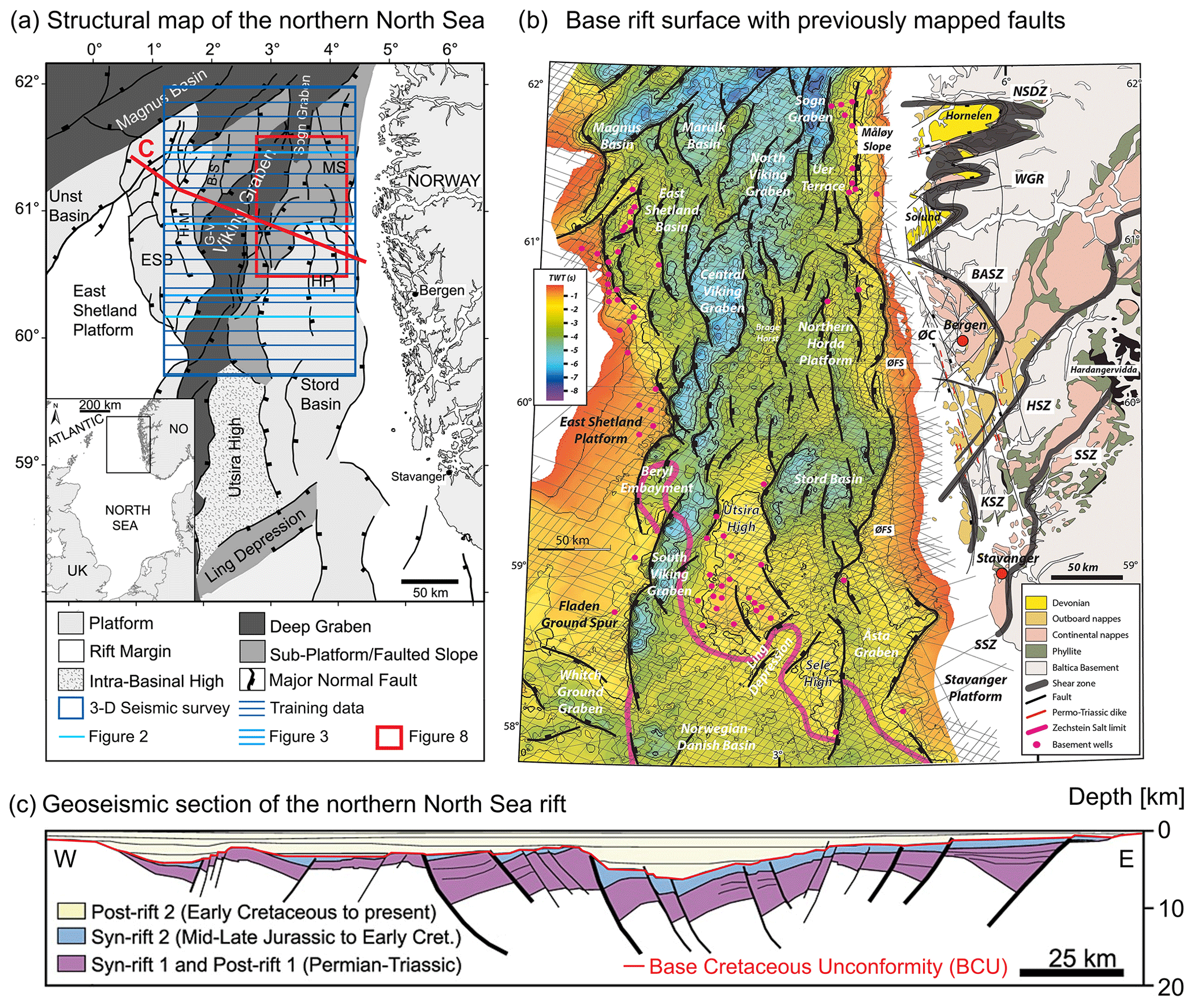
Figure 1 (a) Structural overview map of the northern North Sea basin system (from Tillmans et al., 2021, after Færseth, 1996). The bright blue rectangle marks the outline of the seismic survey in this study. ESB is the East Shetland Basin, B–S is the Brent–Statfjord fault, G–V is the Gullfaks–Visund fault, MS is the Måløy slope and HP is the Horda Platform. (b) The base rift surface (base Permo-Triassic rifting) time–structure map in the northern North Sea rift (from Fazlikhani et al., 2017) and the geology of southwestern Norway, showing the general onshore and offshore structural configuration in the study area. The bold black lines highlight major rift-related normal faults displacing the base rift surface where all units older than upper Permian are considered basement. The black lines in the background show some of the 2-D seismic reflection surveys used by Fazlikhani et al. (2017). NSDZ, Nordfjord–Sogn Detachment Zone; BASZ, Bergen Arc Shear Zone; WGR, Western Gneiss Region; ØC, Øygarden Complex (gneiss); ØFS, Øygarden Fault System; HSZ, KSZ and SSZ: Hardangerfjord, Karmøy and Stavanger shear zones respectively. (c) Regional interpretation of the structure of the northern North Sea after Færseth (1996).

3 Data and methods

3.1 3-D seismic reflection data

In this study, we use one of the largest offshore 3-D seismic data sets ever acquired, which images a large part of the northern North Sea rift across an area of 35 410 km² and with excellent depth imaging down to 22 km (i.e. the middle to lower crust) (Figs. 1, 2a and 3). The data set was acquired using eight streamers that were up to 8 km long and were towed ∼40 m below the water's surface. The BroadSeis technology used for recording covers a wide range of frequencies (2.5–155 Hz), providing high-resolution depth imaging. The data were binned at 12.5×18.75 m, with a vertical sample rate of 4 ms. The data were 3-D true amplitude prestack depth migrated. The seismic volume was zero-phase-processed with SEG (Society of Exploration Geophysicists) normal polarity; i.e. a positive reflection (white) corresponds to an acoustic impedance (density × velocity) increase with depth. More details on data acquisition and pre-processing steps are provided by Wrona et al. (2019, 2021b).

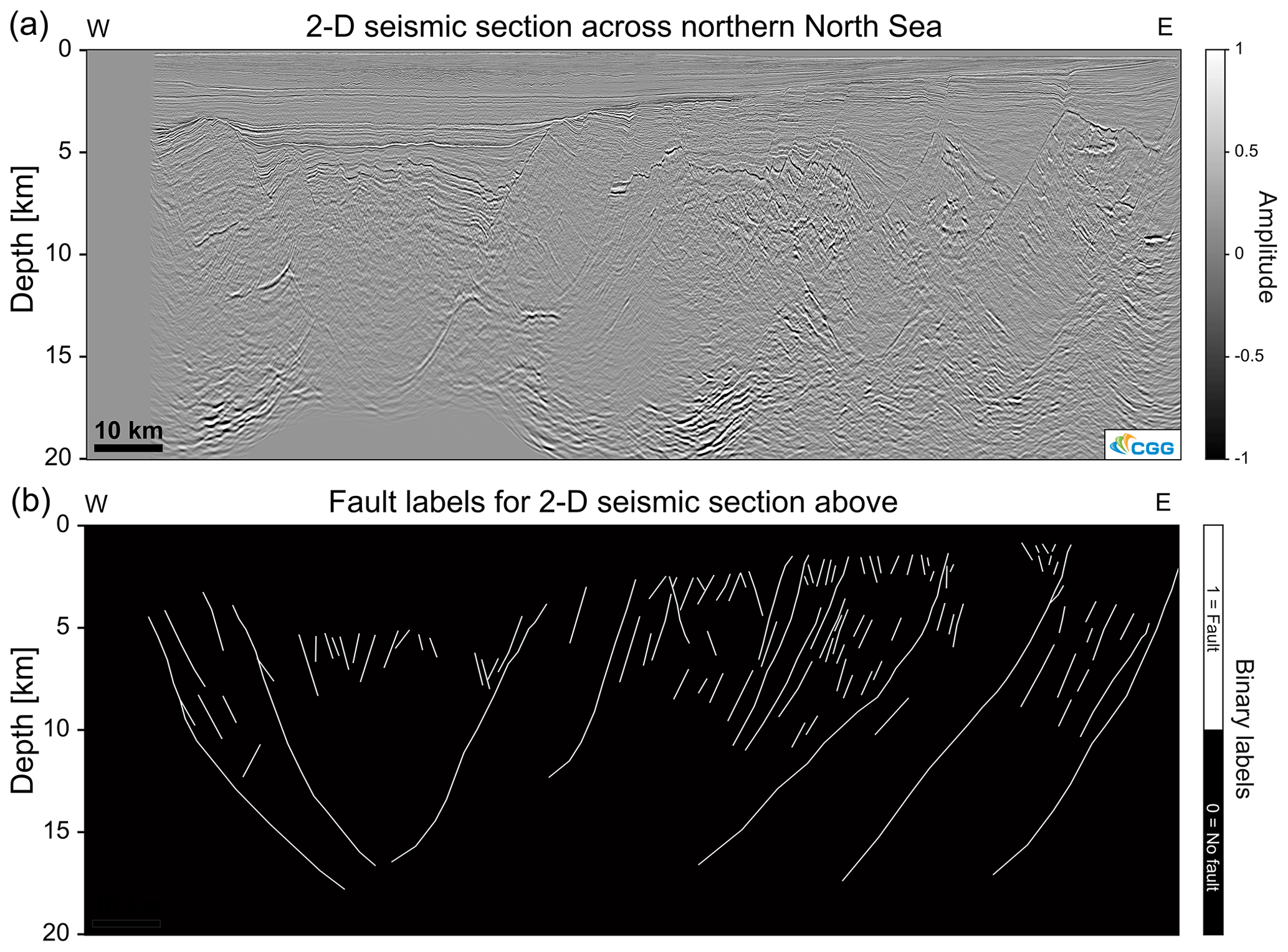
Figure 2 (a) Example of a seismic section across the northern North Sea. Amplitudes are scaled for machine learning. (b) Example of fault interpretation of the section used to train a deep convolutional neural network for fault prediction.

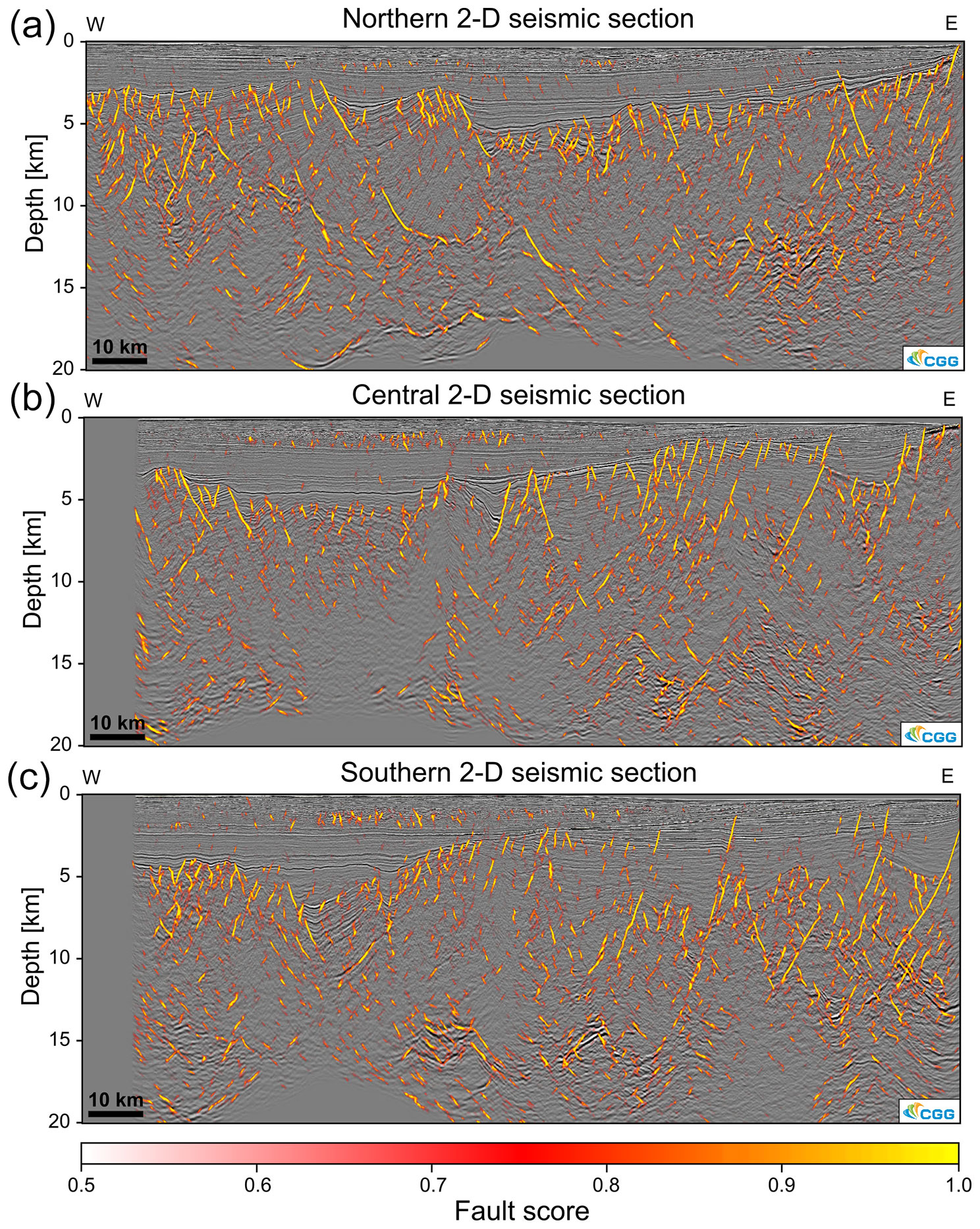
Figure 3 Examples of seismic sections extracted from fault score volume of the 3-D seismic data set. Note that these sections were not part of the training data but are actually 6.25 km away from the closest interpreted seismic section (see Fig. 1a). To show the correspondence between seismic data and fault score, we needed to define a cutoff value (0.5) below which the fault score becomes transparent and the seismic data become visible.

3.2 Deep learning

Deep learning describes a set of algorithms and models which learn to perform a specific task (e.g. fault interpretation) on a given data set without requiring explicit feature engineering (e.g. the calculation and calibration of seismic attributes, such as coherence or variance). Deep learning allows the derivation of a fault score volume that highlights normal faults within the entire 3-D seismic volume. This approach requires a large number of examples of faults and unfaulted strata to be labelled in the training seismic data. We extract 80 000 such examples (2-D squares of 128×128 pixels) from 22 interpreted seismic sections oriented perpendicularly to the N–S-trending rift (Figs. 1a and 2). Note that these seismic sections only constitute <0.1 % of the entire 3-D seismic volume. Next, we split these examples into three groups: one set for training (80 %), one set for validation (10 %) and one set for testing (10 %). We use the first of these groups to train a deep convolutional neural network (U-Net) designed to perform image segmentation tasks (Ronneberger et al., 2015). Using the validation set, we track the accuracy and loss of the model during training and stop once the validation loss does not decrease further, resulting in a final binary accuracy of 0.83 and an F1 score of 0.76 (see Wrona et al., 2021b). Finally, we apply the model to the entire 3-D seismic volume to derive a fault score volume (Figs. 3 and 4), which is an attribute that ranges from 0 (no fault) to 1 (fault). All details of the workflow and the code are provided by Wrona et al. (2021a).

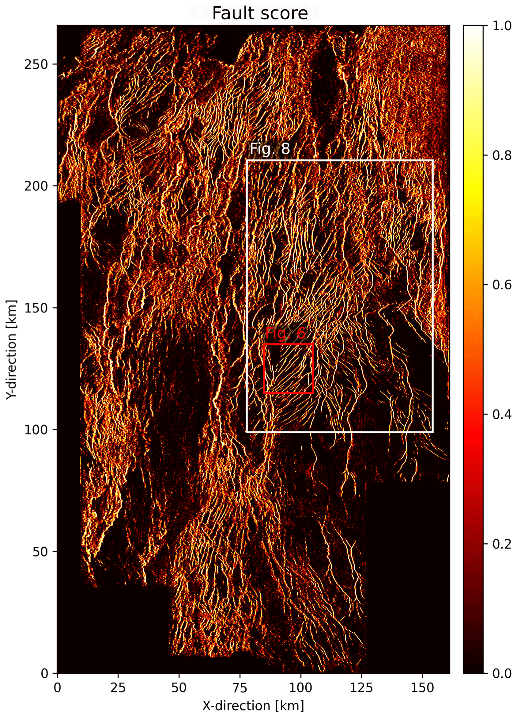
Figure 4 Surface capturing tectonic faults extracted from fault score volume. The surface was extracted 500 m below the Base Cretaceous Unconformity, where we observe a large number of faults, which were either formed or reactivated in the second rift phase. The white rectangle shows the area used for validation (Fig. 8) and the red rectangle indicates the area where we demonstrate our fault network extraction workflow (Fig. 6). Note that this figure shows a whole range of values of the fault score [0, 1].

3.3 Automated fault network extraction and analysis

Extracting a fault network from the 3-D volume allows us to perform a comprehensive geometric analysis of the fault system using our fault analysis toolbox – fatbox (Wrona et al., 2022). The basic idea is to describe a fault system in 2-D as a network (or graph), i.e. sets of nodes and edges (Fig. 5). Each node marks a location along the fault and each edge connects two nodes. All nodes connected to one another by edges are labelled as a (connected) component.

Our fault extraction workflow consists of the following eight steps: (1) extracting a horizon, (2) Gaussian blur filtering, (3) thresholding, (4) cleaning, (5) skeletonisation, (6) connecting components, (7) adding nodes to the graph, (8) adding edges to the graph and (9) splitting junctions. While applying it to our North Sea target region, we first attempt to capture as many faults as possible by extracting the fault score along a horizon 500 m below Base Cretaceous Unconformity (BCU) (Fig. 1c). Here, we observe a large number of faults, which were either formed in the second rift phase or formed in the first rift phase and reactivated in the second rift phase (Figs. 4 and 6a). Second, we apply a Gaussian blur filter to increase lateral fault continuity (Fig. 6b), which allows us to extract long geologically plausible faults. Using a small filter (σ=2) results in local smoothing without connecting distant faults with one another. Third, we apply a threshold of 0.35 to separate the faults from the background in the fault score (Fig. 6c). This threshold is a tradeoff, which balances capturing as many faults as possible (lower values) with identifying clearly resolvable faults (high values). Fourth, we further restrict this threshold and essentially filter these points by removing areas smaller than 25 pixels (Fig. 6d). Fifth, we collapse these faults to 1-pixel-wide lines using skeletonisation (Guo and Hall, 1992) (Fig. 6e). Sixth, we label adjacent pixels in the image as connected components (Wu et al., 2009) (Fig. 6f). Each component consists of pixels which are connected to each other. These components represent the faults in our network. At this point, we can build our graph using these connected components of the image (Fig. 6f). Each pixel that belongs to a component becomes a node, whereas edges are created between neighbouring nodes (Fig. 6g–i). This process results in a number of faults with splays, junctions or intersections being grouped into one connected component (Fig. 7a). To correct this, we split up junctions (nodes with three edges) based on the similarity of the strike; i.e. the aligned branches remain connected (Fig. 7b and c). This final network is compared with the base late Jurassic horizon mapped by Tillmans et al. (2021) (Fig. 8). Additionally, we perform the exact same workflow on 10 slices through the fault score volume (1–10 km depth) to capture 3-D fault geometries with depths (Fig. 9).

After extracting the fault system, we calculate a series of typical fault properties by using our fault analysis toolbox – fatbox (Wrona et al., 2022) (Fig. 10). First, we calculate the fault length as the sum of the edge lengths of each component (Fig. 10b). Second, we calculate the strike along the fault from neighbouring nodes (Fig. 10c). If we were to calculate the overall fault strike, we would overlook along-strike variations in the strike. If we were to calculate the strike as the orientation of each edge, we would only obtain values of 0,45 or 90^∘, because the nodes are closely spaced. Instead, we calculate the strike from the third degree of the neighbouring nodes (i.e. neighbours of neighbours of neighbours). This selection ensures a robust, high-resolution fault strike calculation. Combining the fault length and strike, we can generate a length-weighted rose diagram (Fig. 10c). Finally, we calculate the fault density as the fault length per area (Fig. 10d).

3.4 Comparison to conventional seismic interpretation

We can ask ourselves, “how good are our results compared to a state-of-the-art fault interpretation from the same data set using conventional fault mapping techniques?” (Fig. 8). Tillmans et al. (2021) map the base late Jurassic (base of syn-rift sediments associated with rift phase 2) on the eastern flank of the North Viking Graben (see Figs. 1a and 4 for location), using a combination of manual picking and auto-tracking on the same seismic data set. This horizon is calibrated with 40 exploration wells, which provide direct constraints on the depth of the surface. Tillmans et al. (2021) highlight the fault system by computing the variance attribute (Chopra and Marfurt, 2007) along the horizon (Fig. 7a). On top of the horizon, we plot the fault network that was mapped from the fault score extracted 500 m below the easily mappable Base Cretaceous Unconformity (BCU) (Fig. 8b). This visual comparison shows that, while we are missing a few faults in the southwest of the map, we are able to identify and accurately represent most of the faults identified by Tillmans et al. (2021). The missing faults are either overlooked by our model (i.e. false negatives) or result from the difference between the horizons that we compare: Base Cretaceous Unconformity (our study) versus base late Jurassic (Tillmans et al., 2021).

4 Observations

Our fault extraction allows us to map a complex network consisting of 7983 individual faults across an area approximately 161 km wide and 266 km long, covering 35 410 km² of the northern North Sea rift (Fig. 7c).

4.1 Fault length

Faults vary in length by 3 orders of magnitude – from 50 m to 75.9 km – with some of the longest faults (>30 km) extending from the Stord Basin and Bjørgvin Arch in the south to the Uer and Lomre terraces in the north (Fig. 10b). In the cross section, these faults have up to several kilometres of displacement and bound rotated half-graben (e.g. Whipp et al., 2014; Bell et al., 2014) (Fig. 3b and c). While we observe some long (up to 20 km) faults in the Viking graben and Tampen Spur, most faults (>90 %) are closely spaced (<5 km) and relatively short (<10 km long) (Fig. 10b).

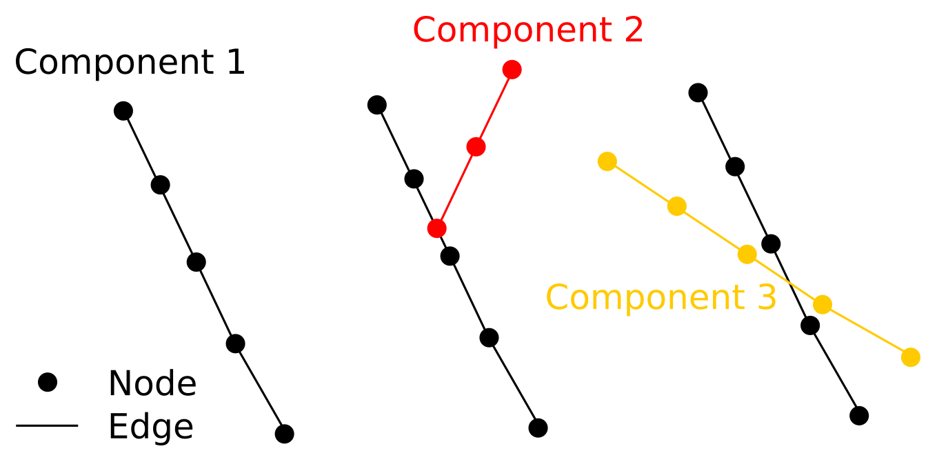
Figure 5 Schematic illustration of fault network (or graph) with nodes, edges and components. Each node marks a location along the fault. Each edge connects two nodes and each (connected) component indicates all nodes connected to one another by edges.

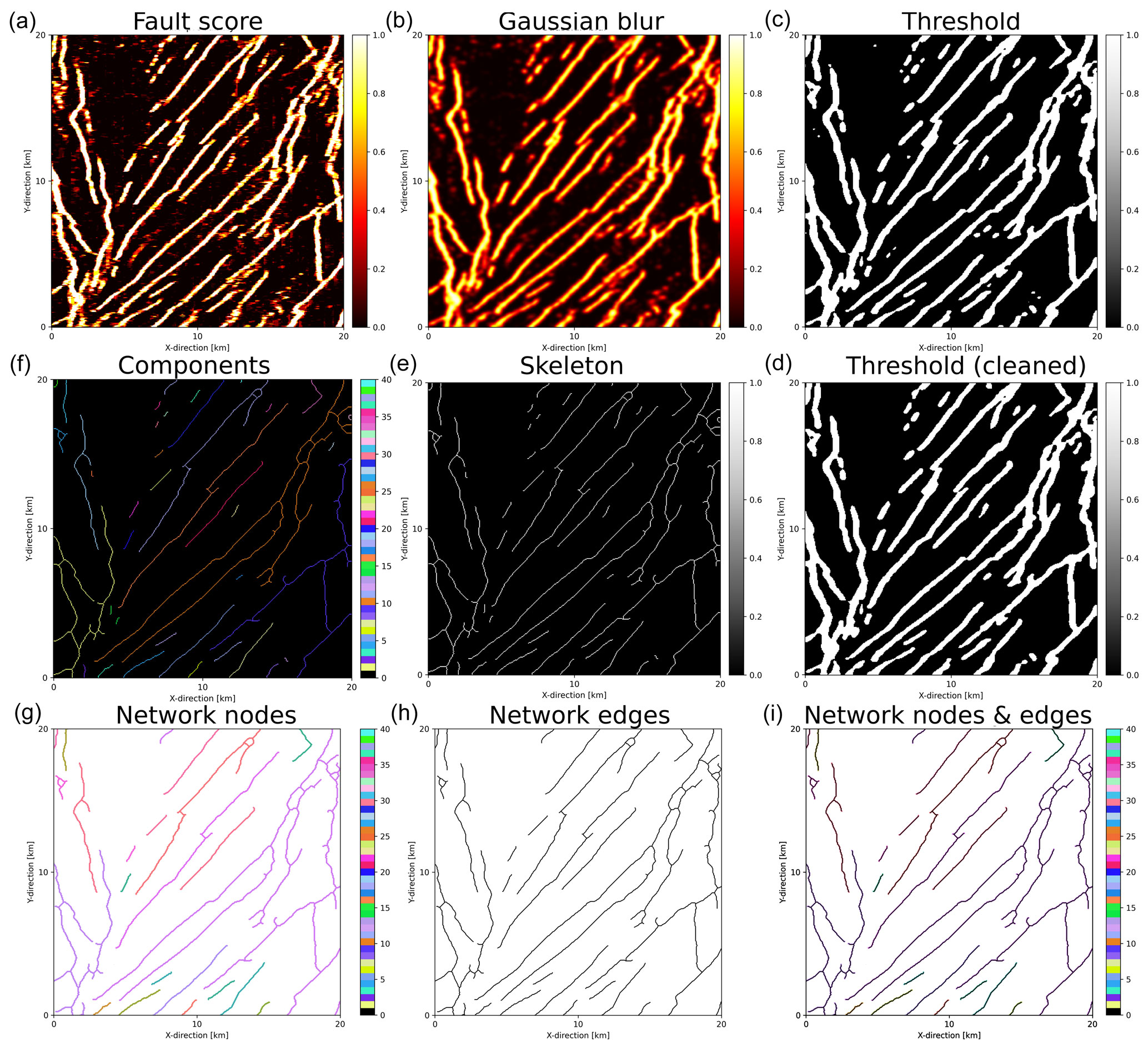
Figure 6 Fault network extraction workflow showing the following: (a) fault score extracted along the surface (500 m below BCU), (b) Gaussian blur filter (σ=2) of surface, (c) threshold (0.35) of filter, (d) cleaned threshold where small patches are removed, (e) skeleton of cleaned threshold, (f) connected components of skeleton, (g) network nodes based on components, (h) network edges based on components, and (i) network nodes and edges combined. Note that the colours in (f), (g) and (i) indicate connected components (i.e. individual faults), before splitting (see Fig. 6).

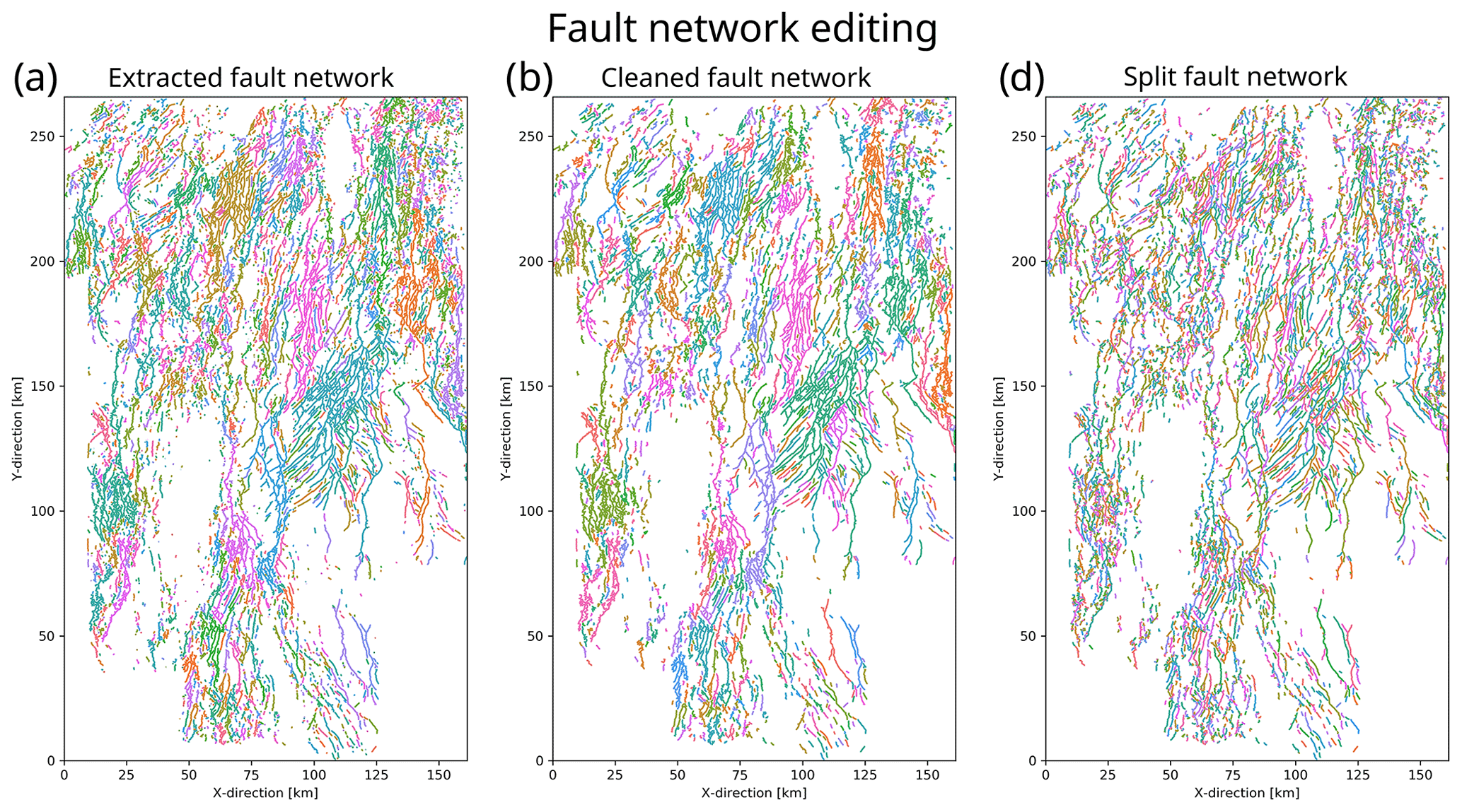
Figure 7 (a) Fault network extracted from BCU (Fig. 4d). Note the large areas with the same colours resulting from multiple faults being grouped into one connected component. (b) Fault network after removal of noise (i.e. small components). (c) Fault network after splitting junctions that previously connected splaying and intersecting faults. Note that large connected components are split up and individual faults are highlighted by different colours.

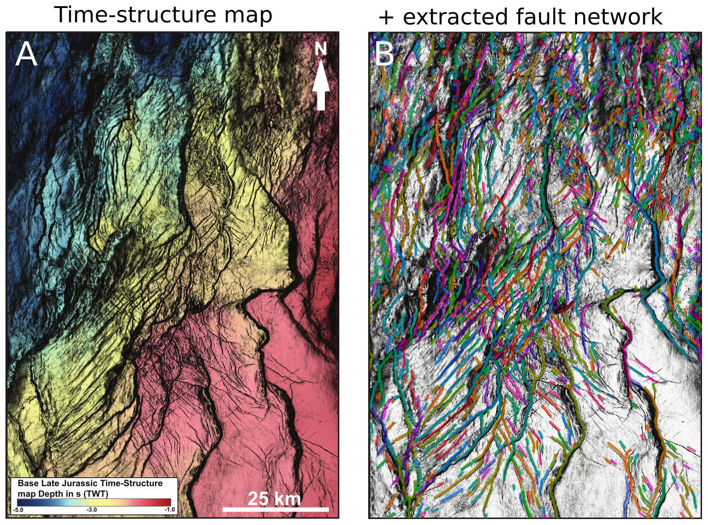
Figure 8 Comparison of panel (a) base late Jurassic time–structure map interpreted by Tillmans et al. (2021) and panel (b) automatically extracted fault network 500 m below Base Cretaceous Unconformity, using the same seismic data set. Faults are distinguished by colour.

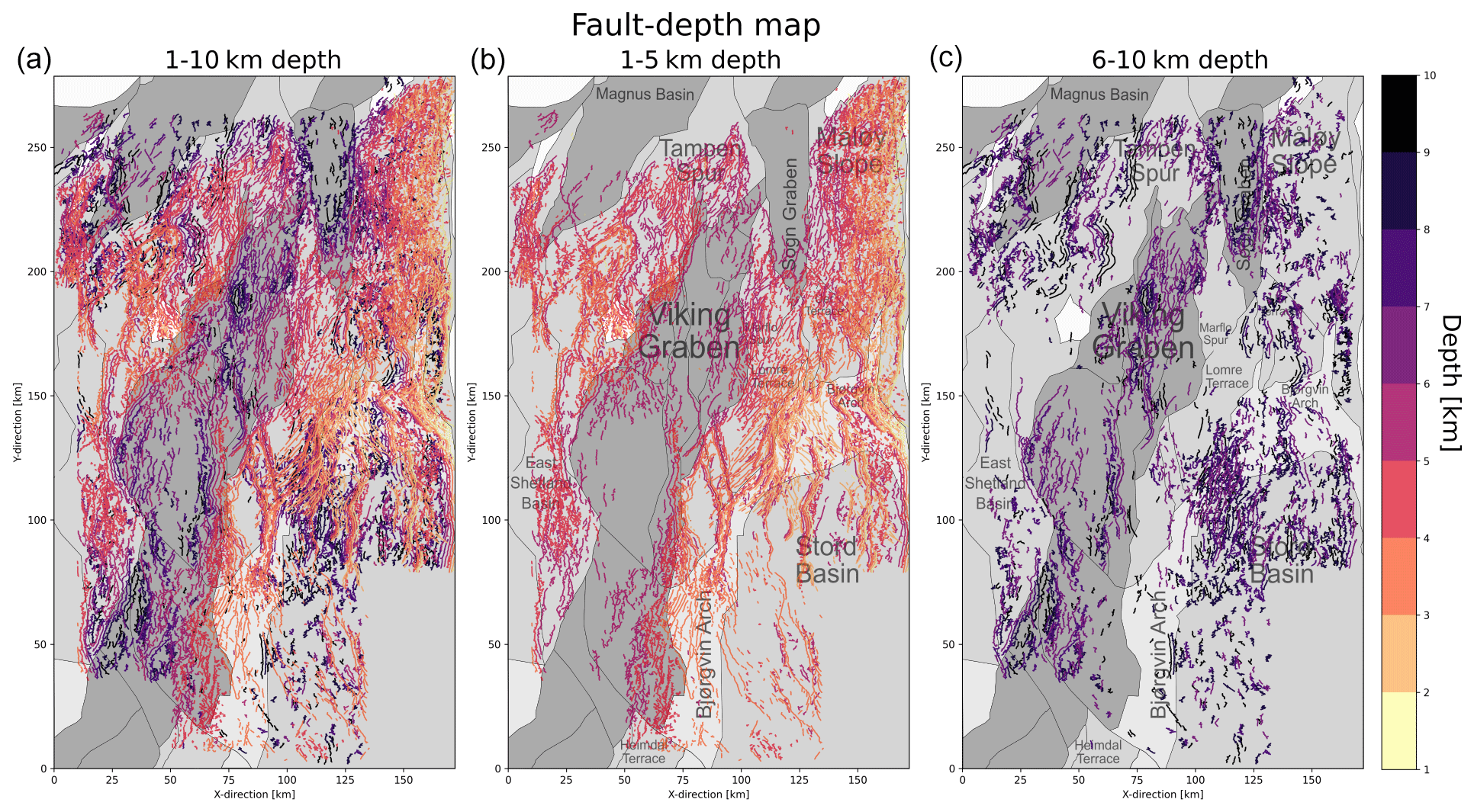
Figure 9 Fault map of the northern North Sea extracted every kilometre from (a) 1–10 km depth, (b) 1–5 km depth and (c) 6–10 km depth, with structural elements from the Norwegian Petroleum Directorate or NPD (2022).

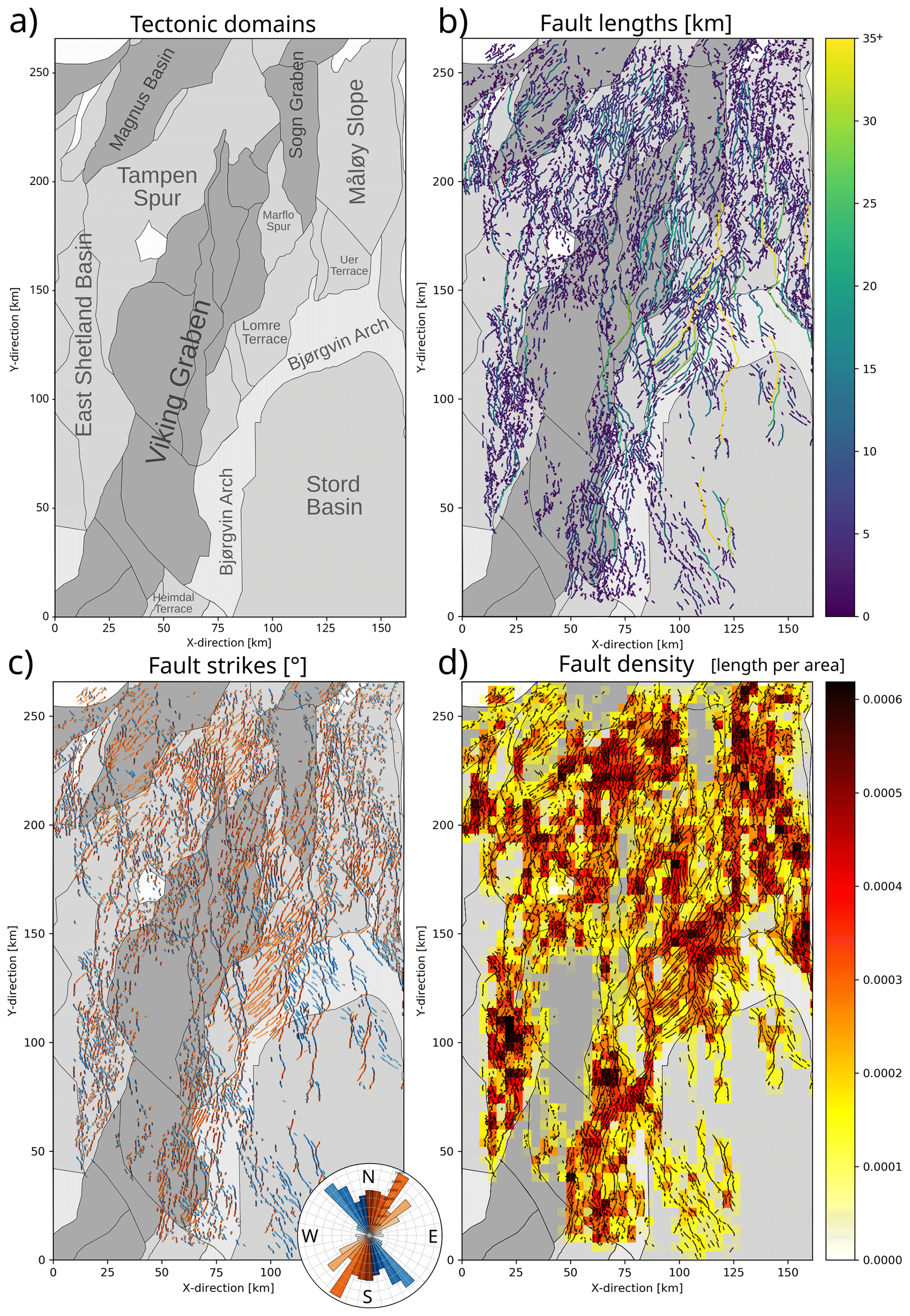
Figure 10 (a) Structural elements of the northern North Sea Rift (NPD, 2022). (b) Fault lengths (500 m below BCU) on top of structural elements. (c) Fault strikes (500 m below BCU) on top of structural elements with length-weighted rose diagram. (d) Fault density on top of structural elements. Note that fault density was measured as fault length per square area. These squares have an edge length of 3.6 km, a value chosen for visual purposes.

4.2 Fault strikes

In map view, we observe a complex network consisting of a large number of variably trending faults that display a broad range of intersection styles (e.g. oblique and perpendicular). These faults show a large range of strikes, varying from NW–SE to NE–SW (Figs. 9 and 10c). The length-weighted rose plot shows that most faults strike NW–SE (light blue) or NNE–SSW (light orange), with a large number of faults showing intervening strike directions (Fig. 10c). This general divide occurs between predominantly NW–SE-striking faults along the eastern part of the rift and NE–SW-striking faults in the central and northwestern part of the rift. This divide becomes most evident when comparing the faults on the Lomre Terrace (NE–SW) with the faults on the adjacent Bjørgvin Arch (NW–SE), at least at the structural level of the Base Cretaceous Unconformity (Fig. 10c).

4.3 Fault density

In map view, we observe large variations in fault density 500 below the BCU (Fig. 10d). While dense networks of intersecting faults result in high-density areas (e.g.  the Lomre Terrace and Bjørgvin Arch), we observe low densities in the Viking and Sogn grabens, where faults occur at greater depths (e.g. Fig. 9c).

4.4 Vertical continuity

The faults extracted at different depths are variable in their vertical continuity (i.e. fault height; Fig. 8). Whereas some faults, in particular in the Stord Basin, the Tampen Spur and the Magnus Basin, show parallel fault traces from 1 to 10 km depth (Fig. 9a), we also observe a large number of faults that occur only at shallower (1–5 km) or greater depths (6–10 km) (Fig. 9b and c). Upon closer inspection, we observe that the faults, which occur continuously from 1–10 km depth (e.g. in the eastern Stord Basin and the Bjørgvin Arch), are typically large-displacement normal faults with tens of kilometres of spacing (e.g. Fig. 3b and c), whereas the other faults, which only occur from 6–10 km depth (e.g. the northwestern Stord Basin), are usually shorter and more closely spaced (a few kilometres) (e.g. Fig. 9c).

5 Discussion

5.1 Advantages of deep-learning-based fault interpretation

When comparing our results to conventional interpretation methods, we can ask ourselves, “what value does deep learning add?” Here, we highlight the advantages of the supervised deep-learning-based fault interpretation workflow, which we present in this study. First, we can predict faults in a seismic section in a fraction of the time (5 s) required by expert interpreters (∼10 min). These differences accumulate, in particular, when interpreting such a large data set with >22 000 inlines. A conventional fault interpretation of such a large data set can take several months, whereas a trained convolutional neural network can identify faults across the entire volume within a day on a single GPU (GeForce GTX 1080 ti). Note that this comparison does not include the time required to label the training data (∼2 d), train the initial model (∼4 h), and fine-tune and select the final model (days–months). Second, after identifying faults in the data, they also need to be mapped before we can perform the relevant fault analysis. Here, we map the fault network using a series of tools from computer vision and network analyses compiled in our fault analysis toolbox – fatbox (Wrona et al., 2022) (Figs. 6 and 7). Our automated workflow extracts the fault network in less than 5 min compared with the several weeks to months that would have been required to manually map the faults in this large data set. Furthermore, once extracted, we can immediately conduct a number of typical fault analyses using predefined functions implemented in fatbox (Wrona et al., 2022) (e.g. Fig. 10).

Third, conventional fault interpretations are often binary (fault vs. no fault), but deep learning delivers a score ranging from 0 (no fault) to 1 (fault). Although this score is not a true fault probability (see discussion by Mosser and Zabihi Naeini, 2022), the fault score nevertheless correlates with the visibility of faults (i.e. the faults which are well resolved by the data are associated with higher fault scores). This correlation allows users to qualitatively select the faults that they want to analyse by using a threshold (as done herein). This selection is particularly useful for assessing the sealing potential of certain layers for CO₂ storage and predicting fluid flow during geothermal exploration. Fourth, seismic interpreters typically focus on the largest faults, whereas our model performs the same prediction across the entire data set, irrespective of the size of the faults encountered. Fifth, given the same data, labels, model and training, our model and results are fully reproducible, which is not the case for conventional fault interpretations, where the interpreter has to make a myriad of decisions in the process of mapping a fault network.

5.2 Complex fault system in the northern North Sea

Our study shows how to reveal the complex geometry of normal fault systems in 3-D seismic reflection data, using a combination of deep learning and automated fault extraction. We were able to map an intricate network consisting of almost 8000 individual faults that cover an area approximately 161 km wide and 266 km long (e.g. Figs. 4, 6 and 10). This fault network shows large variations in the fault length, strike and density, with extremely complex splays, junctions and intersections between these faults (Figs. 7–11). As such, our work goes far beyond the typical seismic interpretations in previous case studies, which covered only a fraction of the rift (e.g. Duffy et al., 2015; Deng et al., 2017; Tillmans et al., 2021), or regional studies that mapped <100 of the largest faults, using primarily sparse, 2-D seismic sections (e.g. Fig. 1b; Fazlikhani et al., 2017; Phillips et al., 2019).

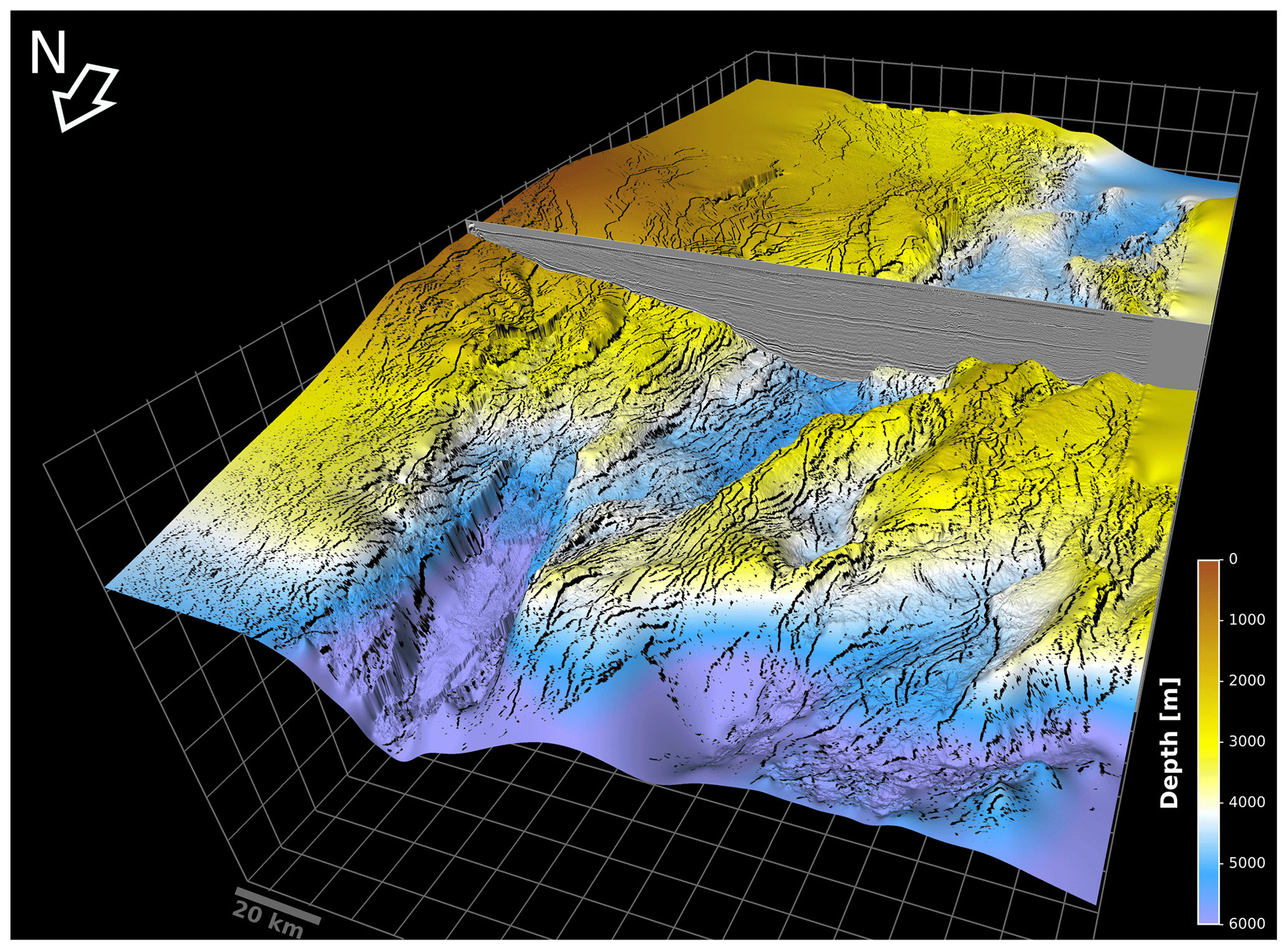
Figure 11 3-D perspective of the northern North Sea rift showing the Base Cretaceous Unconformity overlain with faults (black) extracted from 3-D seismic reflection data with deep learning and a vertical exaggeration of 5.

5.3 Uncertainties during fault mapping

While there are several advantages to our approach, it is worth remembering the uncertainties associated with mapping faults in seismic reflection data. First, seismic reflection data can only image faults with displacement above the seismic resolution (and level of noise) of the data set. The seismic resolution of our data set decreases from 15 m (vertical) and 30 m (lateral) around 3 km depth down to 180 m (vertical) around 20 km depth (see Wrona et al., 2019; Tillmans et al., 2021). Second, the labels we use to train our model are derived from 22 interpreted seismic sections, which, like any seismic interpretation, contain the expertise and biases of the interpreter (e.g. Bond et al., 2007; Bond, 2015). Third, our current model has not been trained and is, thus, unable to distinguish between different fault types (normal, reverse and strike-slip). We labelled all major faults in the training data, which are predominantly normal faults (probably >99 %). A handful of these normal faults may show evidence of minor inversion, but they all remain in net extension; i.e. the hanging wall has moved down relative to the footwall. While strike-slip faults are notoriously difficult to resolve in seismic reflection data, as they show little to no vertical offset of reflectors, the normal and reverse faults show differing offsets, which neural networks could learn to recognise by correlating reflectors across the fault. Machine learning models could, thus, be able to distinguish fault types based on their seismic signature in the future. Fourth, the convolutional neural network that we trained achieves an accuracy of 83 %, implying that 17 % of the data are misclassified (see Wrona et al., 2021b). A closer inspection reveals that 36 % are false positives (i.e. the faults that were overlooked) and 5 % are false negatives (i.e. the faults that were misinterpreted) (see Wrona et al., 2021b). Despite these limitations, the robustness of our approach is evident when considering along-strike fault continuity across a large number of different seismic lines (Figs. 10 and 11).

5.4 Future research on automated fault mapping

Based on our work, we can identify three related areas for future research. First, conventional neural networks predict a fault score from 0 to 1, which seems to correspond to the visibility of the fault in the data set. Bayesian neural networks, on the other hand, allow the prediction of true fault probabilities (e.g. Mosser et al., 2020). Predicting fault probabilities in regional seismic data sets could significantly accelerate the screening for, and risk assessment of, potential CO₂ storage sites (see Wrona and Pan, 2021). Second, we currently map faults on seismic in- and crosslines, which may contain redundant information regarding the faults. In the future, it may be advantageous to maximise the diversity of the training set (i.e. different fault types or levels of noise), using uncertain estimates and active learning. Third, in addition to predicting where faults will occur, we can explore the prediction of other fault properties, such as displacement, fault zone permeability or even the time when they were active. This would allow us to significantly study the spatial and temporal evolution of fault systems in high resolution at a regional scale. Fourth, while our fault extraction workflow currently focuses on mapping fault networks in a series of 2-D slices or horizons, we really need freely available methods to generate 3-D fault surfaces, which allow for complex fault splays, junctions and intersections, as they could be applied to large 3-D seismic data sets but also to analogue and numerical models.

6 Conclusions

This study shows that the combination of deep learning and network analysis applied to 3-D seismic reflection data allows us to map almost 8000 normal faults across the entire northern North Sea rift, for the first time. These faults form an intricate network with complex relationships (e.g. splays, junctions and intersections) including large variations in the fault length (50 m to 75.9 km) and strikes (NW–SE to NE–SW). As such, this work goes far beyond previous seismic studies by providing high-resolution fault maps at a regional scale in a fraction of the time required by conventional interpretation methods.