A borehole trajectory inversion scheme to adjust the measurement geometry for 3D travel-time tomography on glaciers

Cross-borehole seismic tomography is a powerful tool to investigate the subsurface with a very high spatial resolution. In a set of boreholes, comprehensive three-dimensional investigations at different depths can be conducted to analyse velocity anisotropy effects due to local changes within the medium. Especially in glaciological applications, the drilling of boreholes with hot water is cost-efficient and provides rapid access to the internal structure of the ice. In turn, movements of the subsurface such as the continuous flow of ice masses cause deformations of the boreholes and complicate a precise determination of the source and receiver positions along the borehole trajectories. Here, we present a three-dimensional inversion scheme that considers the deviations of the boreholes as additional model parameters next to the common velocity inversion parameters. Instead of introducing individual parameters for each source and receiver position, we describe the borehole trajectory with two orthogonal polynomials and only invert for the polynomial coefficients. This significantly reduces the number of additional model parameters and leads to much more stable inversion results. In addition, we also discuss whether the inversion of the borehole parameters can be separated from the velocity inversion, which would enhance the flexibility of our inversion scheme. In that case, updates of the borehole trajectories are only performed if this further reduces the overall error in the data sets. We apply this sequential inversion scheme to a synthetic data set and a field data set from a temperate Alpine glacier. With the sequential inversion, the number of artefacts in the velocity model decreases compared to a velocity inversion without borehole adjustments. In combination with a rough approximation of the borehole trajectories, for example, from additional a priori information, heterogeneities in the velocity model can be imaged similarly to an inversion with fully correct borehole coordinates. Furthermore, we discuss the advantages and limitations of our approach in the context of an inherent seismic anisotropy of the medium and extend our algorithm to consider an elliptic velocity anisotropy. With this extended version of the algorithm, we analyse the interference between a seismic anisotropy in the medium and the borehole coordinate adjustment. Our analysis indicates that the borehole inversion interferes with seismic velocity anisotropy. The inversion can compensate for such a velocity anisotropy. Based on the modelling results, we propose considering polynomials up to degree 3. For such a borehole trajectory inversion, third-order polynomials are a good compromise between a good representation of the true borehole trajectories and minimising compensation for velocity anisotropy.

1 Introduction

Cross-borehole travel-time tomography, based on seismic or ground-penetrating radar (GPR) waves, is widely used to investigate small-scale variations of the subsurface, especially when surface-based experiments suffer from poor resolution. The main advantage is the much higher ray coverage within the target area, allowing a more detailed analysis of small-scale variations of geological heterogeneities. The first experiments with seismic sources were described by Bois et al. (1972) and Menke (1984) and successfully applied in a large number of studies in the last decades. Cross-hole tomography has been used in mining exploration (Wong, 2000), aquifer delineation, and hydrology-related topics (Hubbard and Rubin, 2000; Daley et al., 2004; Dietrich and Tronicke, 2009; Linder et al., 2010; von Ketelhodt et al., 2018). It has also been used to characterise a host rock and its small-scale structures such as fault planes (Maurer and Green, 1997; Rumpf and Tronicke, 2014; Schmelzbach et al., 2016; Doetsch et al., 2020; Shakas et al., 2020) and to investigate pore pressure variations in aquifers and caprocks (Daley et al., 2008; Marchesini et al., 2017; Grab et al., 2022) as well as voids in karst regions (Duan et al., 2017; Kulich and Bleibinhaus, 2020; Peng et al., 2021). Furthermore, Gusmeroli et al. (2010) and Axtell et al. (2016) used GPR-based travel-time tomography to estimate the water content in a polythermal glacier.

In contrast to surface-based experiments, the sources and receivers are usually not directly accessible. In general, the borehole geometry is assumed to be well-known, which allows a correct calculation of distances between sources and receivers. For this purpose, inclinometer and caliper measurements are required to describe the actual borehole geometry, and centralisers have been used to precisely position the tools in the centre of the boreholes. Nevertheless, there are some applications for which such estimates are not feasible. For example, for glaciological applications as described in Axtell et al. (2016), boreholes are usually drilled by using hot-water (Iken, 1988) or steam drills (Heucke, 1999). These are highly efficient and cheap methods for glaciology-related investigations, but they come at the cost of the boreholes having a variable diameter. The upper part of the hole is exposed to hot water for a much longer time than the deepest parts of the boreholes, leading to a rather conical shape of the boreholes. Furthermore, outbreaks due to impurities, meltwater intrusions, and air content that change the thermal capacity as well as a variable drilling speed further complicate the borehole shape. In those boreholes, centralisers usually cannot be used, and the actual position of the instruments may vary around the assumed position (Schwerzmann et al., 2006; Axtell et al., 2016). Furthermore, glaciers constantly move during the time of measurements, especially for comprehensive 3D experiments, which may last days or weeks; this leads to larger deformations of the boreholes over time, and the assumed distances are no longer correct. Although repeated inclinometer measurements may reduce the errors, the required precision may still not be reached.

Dyer and Worthington (1988) and Maurer (1996) have already shown the significant effect of wrong source and receiver coordinates on travel-time inversions. Artefacts have been introduced in the resulting velocities, leading to a misinterpretation of the measurements. They proposed adjusted inversion algorithms that consider the coordinates to be additional model parameters and also invert for the coordinates in a 2D inversion. More recently, Kim and Pyun (2020) developed an approach using full-waveform inversion and a grid-search algorithm to update the 2D receiver coordinates after each step of velocity inversion for a data set from vertical seismic profiling (VSP) experiments. Coordinates and velocity are inverted in two separate steps, allowing a more focused adjustment of different physical parameters.

In general, the majority of tomography measurements only consider 2D applications. This requires the calculation of a 2D tomographic plane that contains the boreholes. Irving et al. (2007) developed a coordinate rotation algorithm to minimise the sum of out-of-plane deviations for sources and receivers. Nevertheless, 2D tomography results do not consider off-plane effects, and even when the results of several 2D planes are combined in the end, the individual inversions do not account for all of the 3D information. Therefore, several 3D inversion schemes have been developed in the last years (Washbourne et al., 2002; Cheng et al., 2016), showing the advantages of a 3D inversion over a combination of individual 2D inversions.

However, for 3D inversions, borehole trace corrections are more complex due to the additional degrees of freedom. Bergman et al. (2004) proposed a method for 3D tomography experiments that implements a static correction term for each receiver to absorb short-wavelength variations in layered subsurface, but other approaches that are successful for 2D inversions (e.g. Maurer, 1996) are difficult to transfer to 3D as the inversion scheme is severely underdetermined. This may lead, for example, to oscillations of the coordinates at larger depths.

This issue becomes even more complicated when considering a subsurface with a certain velocity anisotropy. In glaciers, the ice crystals interact with the flow of the ice mass. The strain conditions in the glacier force the ice crystals (that is, the c axes as the symmetry axis of the hexagonal ice grains) to align in a certain crystal orientation fabric (COF) pattern in accordance with the given stress conditions (e.g. Duval et al., 1983; Alley, 1988). In a compressional regime in polar ice, single maxima have been observed in a variety of ice cores and geophysical experiments (e.g. Azuma and Higashi, 1985). The COF-derived seismic anisotropy effect was initially investigated by Bentley (1972). Diez and Eisen (2015) analysed the effect on seismic velocities for different COF patterns and found an anisotropy of up to 6 % for P waves. For temperate glaciers, older and more recent studies have observed multi-maxima for compressional regimes (Kamb, 1959; Rigsby, 1960; Hellmann et al., 2021b; Monz et al., 2021). Hellmann et al. (2021a) have calculated an azimuthally dependent anisotropy of 2.3 % as a result of such a multi-maximum. Media with such a degree of anisotropy are considered weakly anisotropic. Thomsen (1986) analysed the effect of weak anisotropy on seismic wave propagation and provided linearised equations for seismic velocities by introducing a set of five parameters describing the strength and direction of anisotropy. Later, other studies developed approaches to further describe the anisotropy in specific media with certain anisotropy patterns or fracture orientations and provided ways to implement such anisotropy in existing algorithms (e.g. Faria and Stoffa, 1994; Zhou and Greenhalgh, 2005; Martins, 2006; Chen et al., 2017; Meléndez et al., 2019; Pan et al., 2021). In particular, Zhou et al. (2008) demonstrated the effect of anisotropy on cross-hole travel-time tomography results for tilted transversely isotropic media. The outcome of all these studies is that velocity anisotropy has to be considered to have an influence on the velocities obtained from travel-time tomography.

In this study, we propose an approach for travel-time tomography that is explicitly designed for glaciological experiments and apply this to a multi-cross-hole seismic data set acquired on Rhonegletscher as a case study. The continuous but not necessarily linear movement and ice melt of the glacier during data acquisition caused a deviation of the holes, leading to uncertainties about the particular source and receiver coordinates. Inclinometer measurements at the beginning and end of the campaign provide some constraints considered in the inversion. At the same time, we found that the precision of different instruments was not sufficient under the given measurement conditions on glaciers. In some cases, significant deviations occurred between the different instruments, although measurements were carried out one after the other. These observations initially triggered our investigations for a joint velocity and coordinate inversion. However, instead of inverting for the individual source and receiver positions, we assume that the borehole trajectories can be described with two perpendicular 2D polynomials x(z) and y(z). The degree n of the polynomials is used to control the degree of variations along the trajectories. The additional inversion parameters are these polynomial coefficients. Similar to the approach of Kim and Pyun (2020), we then employ a two-step inversion algorithm that inverts for the velocity and the coefficients of the polynomials in alternation. We further investigate and discuss the interdependence between borehole adjustments and the inherent weak velocity anisotropy of the medium.

2 Methodology

The inversion scheme that we apply in this study consists of two parts. The first step is a three-dimensional velocity inversion based on common ray tracing performed on a finite difference grid. Each cell j (i.e. rectangular prism) has a defined velocity, expressed by its reciprocal value of slowness s_j. For a given source–receiver combination i, the travel time through a cell can be calculated from the length l_i,j of the ray through that cell and its associated slowness value s_j. Summing over all N cells between this source–receiver pair results in the travel time t_i, defined as

$$\begin{array}{}\text{(1)}& t_i=\sum _{j=\mathrm{1}}^N{l}_{ij}{s}_j.\end{array}$$

With the measured travel times from cross-borehole experiments t^obs and an initial start model mⁱⁿⁱ for the velocity distribution and the resulting calculated travel times t^cal, the velocities of the cells that are covered by ray paths, which are determined by a ray-tracing algorithm, can be updated iteratively:

$$\begin{array}{}\text{(2)}& {\displaystyle }& {\displaystyle }\mathrm{\Delta }\mathit{d}={\mathit{t}}^{\text{obs}}-{\mathit{t}}^{\text{cal}},\text{(3)}& {\displaystyle }& {\displaystyle }\mathrm{\Delta }\mathit{m}=({\mathbf{G}}^{\mathrm{T}}\mathbf{G}+\mathit{\mu }{\mathbf{W}}_{\mathrm{M}}{)}^{-\mathrm{1}}{\mathbf{G}}^{\mathrm{T}}\mathrm{\Delta }\mathit{d},\text{(4)}& {\displaystyle }& {\displaystyle }{\mathit{m}}^{\text{new}}={\mathit{m}}^{\text{ini}}+\mathrm{\Delta }\mathit{m},\end{array}$$

where the matrix G contains the partial derivatives (sensitivities) $G_{ij}=\frac{\partial d_i}{\partial m_j}$ for each velocity grid cell. The matrix W_M and μ summarise the regularisation (i.e. damping and smoothing) that is required for a stable inversion. Further details about the regularisation are provided, for example, in Maurer et al. (1998).

The second part of our inversion scheme contains a coordinate inversion that accounts for uncertainties about the borehole trajectories. Although inclinometer data are usually available, specific conditions such as a variable borehole diameter or a moving subsurface incorporate uncertainties that significantly affect the velocity inversion and may lead to artefacts complicating an interpretation. An inversion scheme for the individual coordinates $x,y,$ and z for each source and receiver would result in a severely underdetermined problem. This approach with 3(n_S+n_R) unknowns can be replaced by a more robust one when assuming that the sources and receivers in a borehole are aligned along the continuous borehole trajectory. Then, displacements of the sources and receivers can be described by deformations of the trajectory. As a simple mathematical description, we assume that each three-dimensional borehole trajectory can be described by two orthogonal two-dimensional polynomials x=p(z) and y=q(z). The maximum degree n_p of each polynomial is selected by the user according to a priori information or an educated guess. The inversion problem assumes a known mean velocity between each source and receiver, e.g. derived from the estimated velocity from the previous step in the velocity inversion. Then, a second inversion scheme like the one defined in Eq. (3) can be set up. The Jacobian matrix J contains the first derivatives of the data against the new model parameters, i.e. the polynomial coefficients A_j, $j=\mathrm{1},\mathrm{\dots },n_{\mathrm{p}}$,

$$\begin{array}{}\text{(5)}& J_{ij}={\displaystyle \frac{\partial d_i}{\partial A_j}}={\displaystyle \frac{\partial d_i}{\partial r_k}}{\displaystyle \frac{\partial r_k}{\partial A_j}},\end{array}$$

with $k=\mathrm{1},\mathrm{2}$ for the two horizontal and linearly independent directions x=r₁ and y=r₂. For instance, for the polynomial x=p(z) of the source hole,

$$\begin{array}{}\text{(6)}& x=p\left(z\right)=\sum _{j=\mathrm{1}}^{n_{\mathrm{p}}}{A}_j(z-z_{\mathrm{0}}{)}^j,\end{array}$$

the first derivatives ($j=\mathrm{1},\mathrm{\dots },n_{\mathrm{p}}$) for the ith combination of the source ($x_S,y_S,z_S$) and receiver positions ($x_{\mathrm{R}},y_{\mathrm{R}},z_{\mathrm{R}}$) are

$$\begin{array}{}\text{(7)}& \begin{array}{rl}{J}_{ij}& ={\displaystyle \frac{(-\mathrm{1}{)}^{\mathit{\alpha }}}{v}}{\displaystyle \frac{x_{\mathrm{R}}-x_S}{\sqrt{(x_{\mathrm{R}}-x_S{)}^{\mathrm{2}}+(y_{\mathrm{R}}-y_S{)}^{\mathrm{2}}+(z_{\mathrm{R}}-z_S{)}^{\mathrm{2}}}}}\\ & \times (z_S-z_{\mathrm{0}}{)}^j,\end{array}\end{array}$$

where v is the mean velocity between the source and the receiver and α is an exponent that is α=1 for derivatives to the source coordinates and α=2 for derivatives to the receiver coordinates. For the receiver boreholes, (z_S−z₀) needs to be replaced by (z_R−z₀). $(x_{\mathrm{0}},y_{\mathrm{0}},z_{\mathrm{0}})$ is the collar point of the borehole and assumed to be known, e.g. from differential global navigation satellite system (GNSS) measurements, so that the constant term A₀≡0. In addition, the relative position of the sources and receivers along the boreholes is assumed to be known, for example, by measuring the length of the cables of the instruments in the borehole below the collar point. Similarly, this framework can be applied to the polynomial y=q(z). The regularisation term μW_M in Eq. (3) is exchanged with a Tikhonov regularisation, i.e. W_J=μI, with a damping factor μ that can individually be adjusted for each borehole.

There are two options for implementing the two parts of the inversion. The first one is a sequential inversion. During each iteration of the inversion, the updates of velocity and borehole trajectories are computed independently. The second option is an extended system of equations that considers both parts in one large Jacobian matrix. We have tested both options with identical settings and updated coordinates in each step of iteration and could not find significant differences between the two methods for synthetic data sets. However, the sequential inversion seems to be numerically more stable. Furthermore, the most recent update of the velocities is already considered in the current step of iteration, and additional constraints determining whether a borehole trajectory inversion should be performed are easier to evaluate. It also provides more flexibility to decide if an update of the coordinates in the current step of iteration is beneficial and thus applied or skipped. Therefore, we calculated the results in the next sections with the sequential inversion.

3 Experimental setup for the field data acquisition on Rhonegletscher

Initially we encountered the issue of deviating boreholes when acquiring cross-borehole seismic data for anisotropy-related investigations on Rhonegletscher (Rhone glacier), a temperate glacier (ice temperature T ≈ −0.5 ^∘C) in the Swiss Alps. The glacier still covers an area of 15 km² and is flowing in the southern direction at its current terminus (GLAMOS, 2020). For anisotropy investigations, we drilled a set of 13 boreholes (Fig. 1a) about 500 m north of the terminus with a hot-water drilling system (e.g. Iken, 1988) in summer 2018. The boreholes were arranged in a ring with a diameter of 40 m to obtain cross-borehole seismic measurements under different azimuths (i.e. 0, 30, 60, and 90^∘ relative to the ice flow direction). At the borehole location, the glacier was about 100 m thick, and the ice flowed with a surface flow speed of 16 m a⁻¹ in the southeastern direction (Hellmann et al., 2021b). This ice flow velocity decreases with depth, which leads to a continuous deformation of the boreholes over time. At the surface, the ice moved by 1.2 m within the 3 weeks of data acquisition. The positions of the borehole collars and additional geophones along the surface were measured using a high-precision Leica GNSS device in RTK mode. In addition, we used an inclinometer probe from Geotomography GmbH for an estimate of the borehole trajectories after drilling and observed the ongoing deformation with two repeated measurements. An example from borehole BH01 is shown in Fig. 1b. The continuous deformation could not fully be surveyed by just three inclinometer measurements and thus leads to unknown borehole trajectories for intermediate time steps of data acquisition. Nevertheless, the inclinometer measurements could serve as initial estimates for a borehole trajectory inversion.

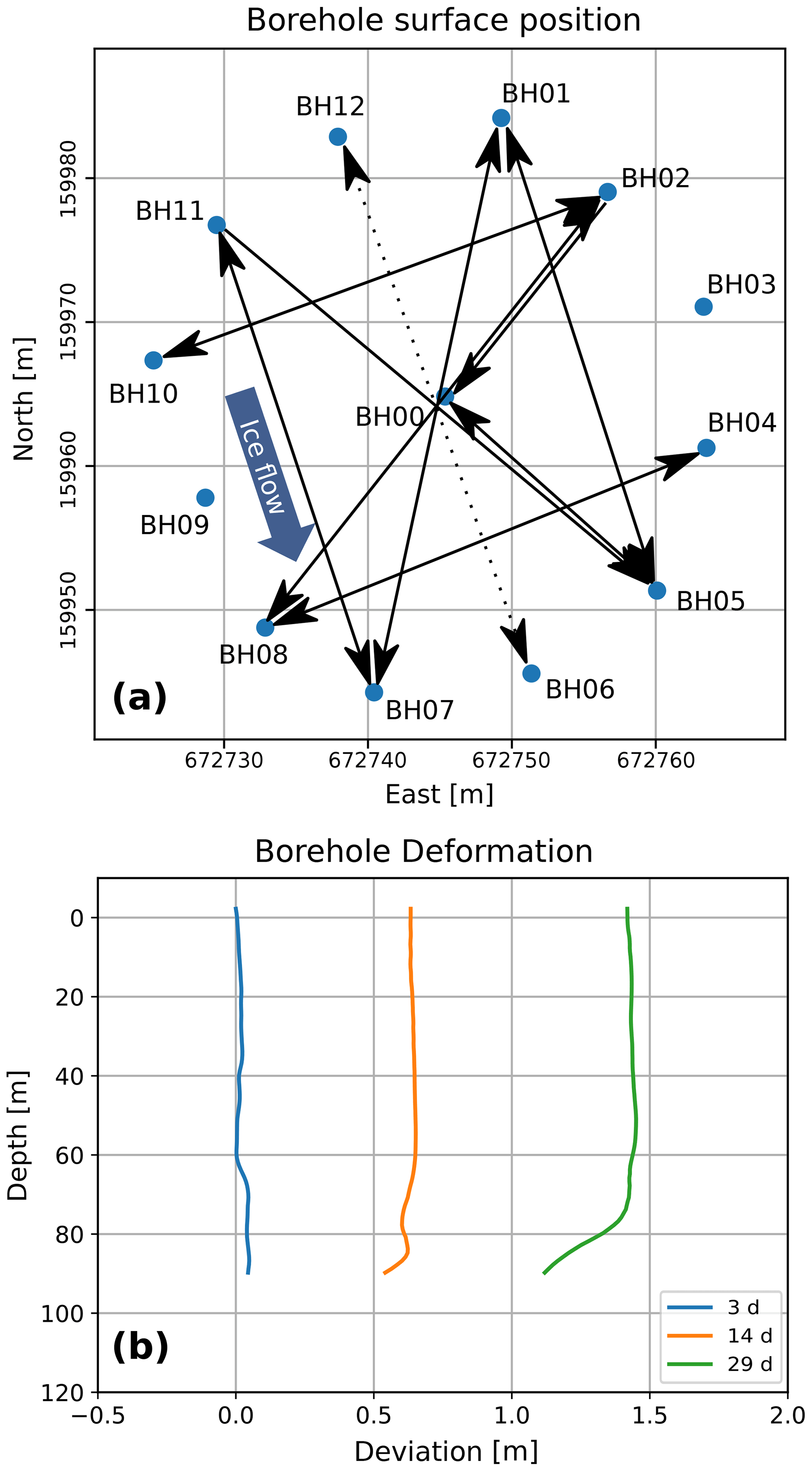
Figure 1 Field data measurement geometry. (a) Positions of the boreholes on the glacier surface (Swiss coordinates, LV03); BH03, BH06, BH09, and BH12 were not used for the experiments shown here. (b) Deformation of borehole BH01 within 4 weeks due to glacier flow.

The continuous displacements and deformations of the glacier ice body are still imposing problems in our attempt to invert simultaneously for subsurface velocities and the borehole trajectories. In principle, the borehole trajectories would have to be estimated for every single source–receiver borehole pair, but this would lead to a poorly constrained inversion problem. To avoid this problem, we have set up our experimental schedule such that every borehole is only occupied for a relatively short time span (up to 4 d). We then made the assumption that the changes in the trajectories are acceptably small within this short time span (i.e. we have inverted for a single trajectory for each borehole). This is certainly a limitation of our methodology, but it is, in our view, an unavoidable compromise that needs to be made.

The drilling of the boreholes was stopped about 15–20 m above the glacier bed to avoid hydrological coupling of the borehole with the subglacial drainage system, resulting in a total borehole length of 80–90 m. For the experimental setup, the boreholes needed to be water-filled. Despite this precaution, borehole BH09 and a second hole just a few metres next to it drained a few minutes after drilling. Similarly, borehole BH11 drained after the second out of 3 d of measurements in this borehole. Since the seismic sparker source and hydrophone receivers can only be deployed in water-filled boreholes, this drainage led to an incomplete data set.

A 5 kV sparker source from Geotomography GmbH with a dominant frequency of 2 kHz was employed in the boreholes for generating the acoustic signal. Hydrophones were installed in the borehole on the opposite side of the ring, as well as in a second borehole either perpendicular or parallel to the glacier flow (Fig. 1a). Geophones, equally spaced at 1 m between the source and receiver boreholes, were placed at the surface of the glacier. These additional receivers further increase the azimuthal resolution of the tomographic experiment. The enhanced ray coverage in the area of investigation reduces the ambiguities between model parameters. This connection of each borehole to two other holes is a prerequisite for the borehole trajectory inversion. Therefore, the exclusively two-dimensional data sets acquired between BH06 and BH12 as well as BH03 and BH00 could not be considered as explained in more detail in Sect. 4.

For sufficiently dense data coverage, we selected a shot interval of 1 m in the source holes as well as a distance of 1 m between the receivers along the surface and within the receiver boreholes. At least three shots were recorded and stacked during the processing to enhance the signal-to-noise ratio. Since the length of the hydrophone chain was limited to 23 m (24 channels), the experiment had to be repeated four times to cover the entire length of the receiver borehole. For the data processing, we applied a standard procedure consisting of a median and bandpass filtering (0.3–15 kHz) to enhance the signal quality, a stacking of repeated shots, and a picking of the P-wave first arrivals with a cross-correlation algorithm. To pick the onset of the P wave, we defined a window around the expected first-break arrival time and analysed the coherency between the traces within the individual receiver gathers. Finally, we performed different combinations of 3D velocity and borehole inversions.

4 Application to a synthetic data set

To demonstrate the effect of our borehole correction, we first applied the approach to a synthetic cross-hole seismic data set. For this purpose, we defined a set of nine boreholes with a length of 80 m. The positions of the borehole collar points were taken from the actual field measurements described in Sect. 3. For the deviations of the boreholes, we fitted a fourth-order polynomial through the data points of the inclinometer measurements and exaggerated this deviation by a factor of 8 to investigate the reliability of our code for cases with even more prominent deviations, e.g. for glaciers with even higher ice flow velocities than those observed on Rhonegletscher. We placed 80 sources and 80 hydrophones in each borehole and added a total of 828 receivers on an inclined plane that represents the surface. These geophones were installed at the glacier surface along 2D lines between the source and receiver boreholes. During data acquisition, about 95 geophones were active at a time, i.e. those along the lines between the currently used boreholes. The geophone positions also refer to GNSS field measurements and were placed 12–20 m below the reference point of the model. The measurement geometry (i.e. the selection of source–receiver profiles) for the synthetic calculations was also based on real field measurements for developing a tool that is suitable for our actual field measurements with a limited number of source–receiver combinations. Therefore, each source hole was connected to only two receiver holes, similar to the profiles shown in Fig. 1a.

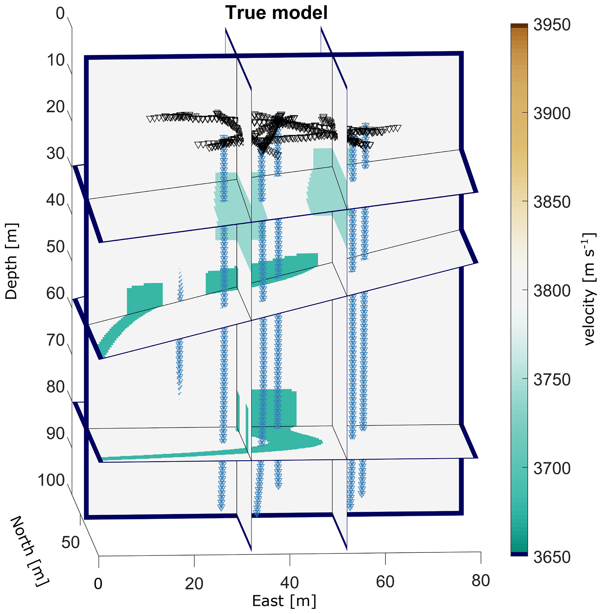
Figure 2 True model of the synthetic example data set with a homogeneous background velocity of 3800 m s⁻¹ and two vertical fault zones with v_p = 3740 m s⁻¹ in the upper part as well as two channels with v_p = 3680 m s⁻¹ in the deeper parts of the model. Triangles and asterisks represent receiver and source positions.

For the investigations, we defined a heterogeneous velocity model (shown in Fig. 2) that consists of the following parts: the background velocity of the true model was set to 3800 m s⁻¹. This value has been measured in ice core samples from Rhonegletscher (Hellmann et al., 2021a), and the cross-borehole field experiments were carried out at the same location. Therefore, we also used this value as the background velocity for our synthetic example. We added two north–south-oriented fault zones (e.g. water-saturated intrusions in the ice) with a slightly lower velocity of 3740 m s⁻¹ close to but below the geophones (z = 20–40 m of the model). In addition, two meandering, inclined structures (representing englacial channels) with a velocity of 3680 m s⁻¹ were included at z = 40–60 and z = 70–86 m. Synthetic data were computed without additional random noise, and they were subsequently inverted using a homogeneous start model with a velocity of 3800 m s⁻¹. Since the tomographic inversion problem includes a significantly underdetermined component, it is necessary to provide regularisation constraints. For the velocity parameters, they were supplied in the form of damping and smoothing constraints (Maurer et al., 1998). After some experimentation, we applied similar weights for damping and smoothing (damping factor of 0.1, smoothing factor of 0.4). We tuned the overall regularisation factor such that the inversions converged to a data misfit level that roughly corresponds to the travel-time picking accuracy. For the model parameters associated with the borehole trajectories, we employed only damping constraints, with which we penalised deviations from the initial values. We started with relatively high damping factors, which we gradually reduced until the inversions became unstable and/or unreasonably large deviations were obtained.

The results of the velocity inversion with correct source and receiver positions are shown in Fig. 3a. The comparison with the true model in terms of velocity differences between the inverted and true model is shown in Fig. 3b. The heterogeneities of the true model could be resolved quite well within the ring of borehole – that is, the area that is covered by the ray paths of the measurements. In turn, this implies that the artefacts in those parts of the model lying outside the ring of boreholes and close to the bottom could therefore not correctly be inverted by any of the inversions and will thus be excluded from the following discussion. This model is regarded as a reference model in the following discussion, although the thickness of the two channels in the lower part of the model and the velocity of the channel between 40 and 60 m are still slightly overestimated. However, these artefacts are most likely a result of the smoothing constraints in the velocity inversion and therefore beyond the scope of our study.

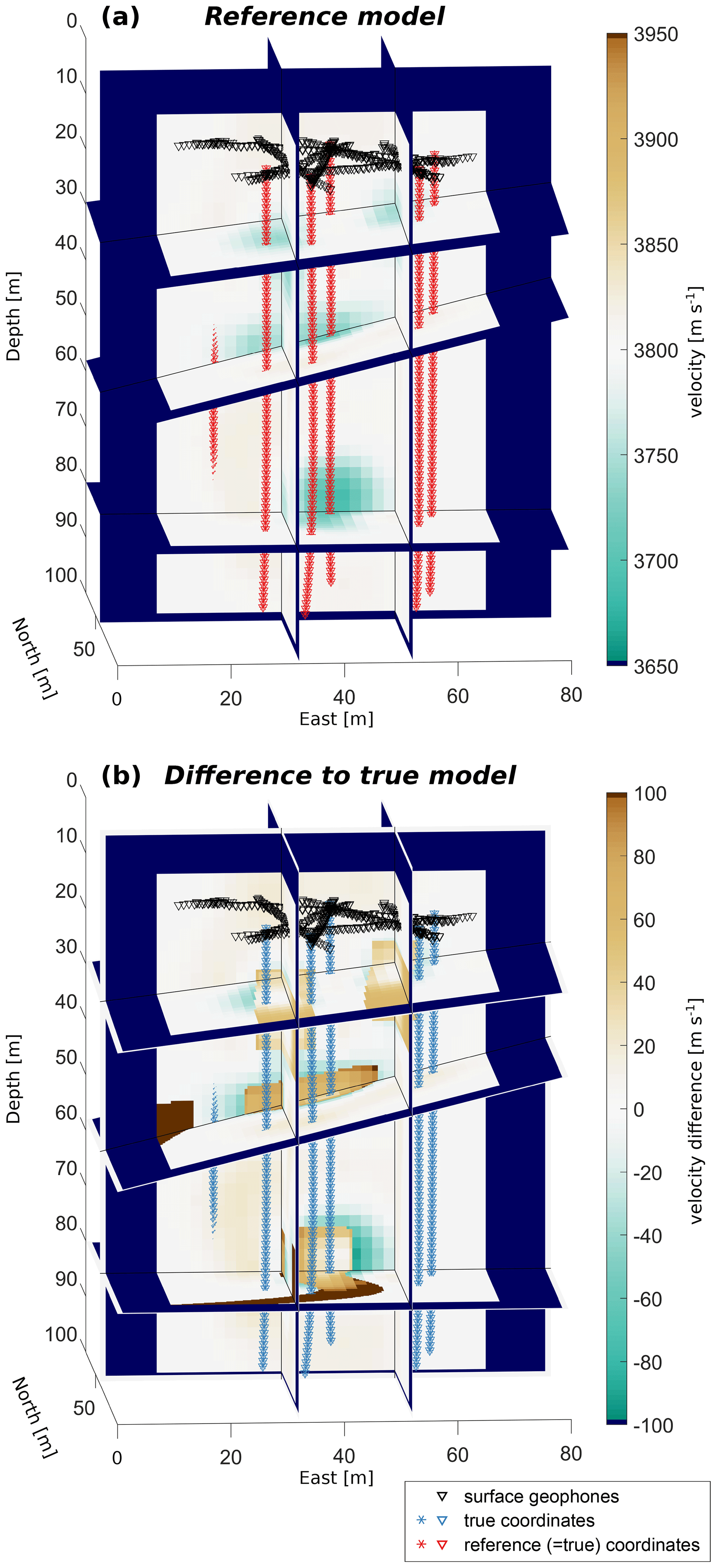
Figure 3 Results of the velocity inversion with a synthetic example data set and correct borehole trajectories: (a) velocity results of the inversion after seven steps of iteration; (b) difference between the inverted and true model (Fig. 2). Triangles and asterisks represent receiver and source positions.

Table 1 RMSEs for the velocity, the combined inversion, and a reference calculation for a velocity inversion with correct trajectories.

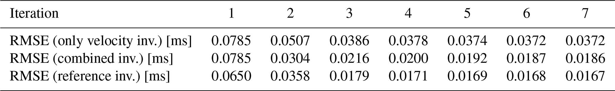
In a next step, the information about the true borehole inclination was ignored and we started with straight vertical boreholes. We ran the inversion without and with borehole trajectory inversion and stopped the inversions after seven iteration steps. Table 1 provides the root mean squared errors (RMSEs) for both inversion schemes. The values provide evidence that these schemes both converge, but the root mean square (rms) values of the sequential inversion are significantly smaller, thus providing a better fit between calculated and measured travel times. Figure 4a shows the inverted velocity model for a pure velocity inversion. The differences to the reference model (Fig. 3) are shown in Fig. 4b. The velocity of the upper and especially the lower channel between 70 and 86 m is only weakly recovered, incorporating clear artefacts in the inversion results (dashed blue ellipses A+B in Fig. 4b). In addition, several artefacts appear at the bottom of the model around the boreholes (see the solid blue ellipses C+D in Fig. 4b showing very prominent examples). This is the region that is covered by only a few measurements and therefore highly underdetermined. Furthermore, the discrepancy between the true inclined boreholes and the assumed straight borehole is the largest at the bottom of the boreholes. As a result, geometrical errors are smeared into the velocity distribution in the least-resolved parts of the model. We also refer to the “Video supplement” (Hellmann, 2022b) for an enhanced overview of the velocity distribution and artefacts in the ice volume.

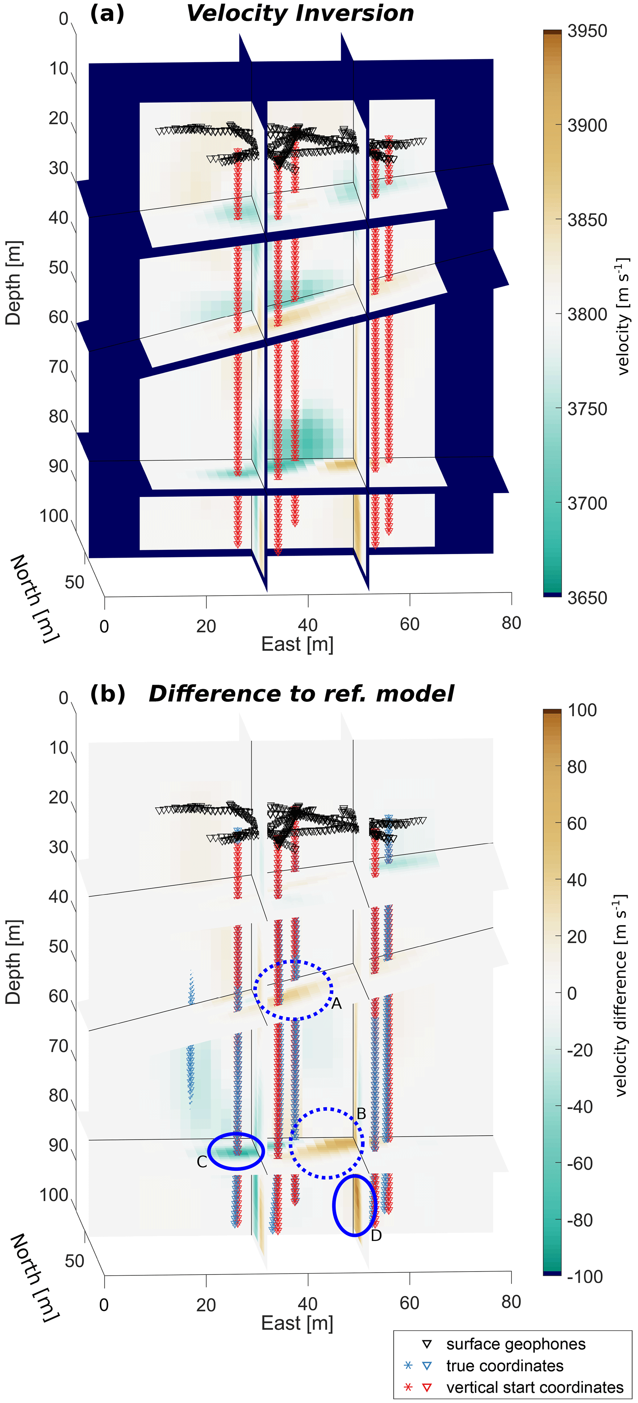
Figure 4 Results of the velocity inversion with a synthetic example data set and initially straight borehole trajectories. (a) Velocity inversion results after seven steps of iteration; (b) difference between inversion results in (a) and the reference model (Fig. 3a), with turquoise ellipses emphasising the most significant differences. Triangles and asterisks represent receiver and source positions.

The calculations for the inversion were repeated with an additional borehole trajectory inversion. Each borehole is approximated by a set of two mutually perpendicular polynomials of degree 4. Figure 5a shows the results of this inversion, and Fig. 5b shows the differences with respect to the reference model. Here, the upper channel and especially the lower channel (ellipses A+B) are correctly resolved with a velocity misfit of < 20 m s⁻¹ inside the channel. In addition, the prominent artefacts in the vicinity of the boreholes and artefacts at the bottom of the model (ellipses C+D) are significantly reduced. Thus, including a trajectory inversion yields results comparable with those in Fig. 3 obtained by using the true borehole geometry.

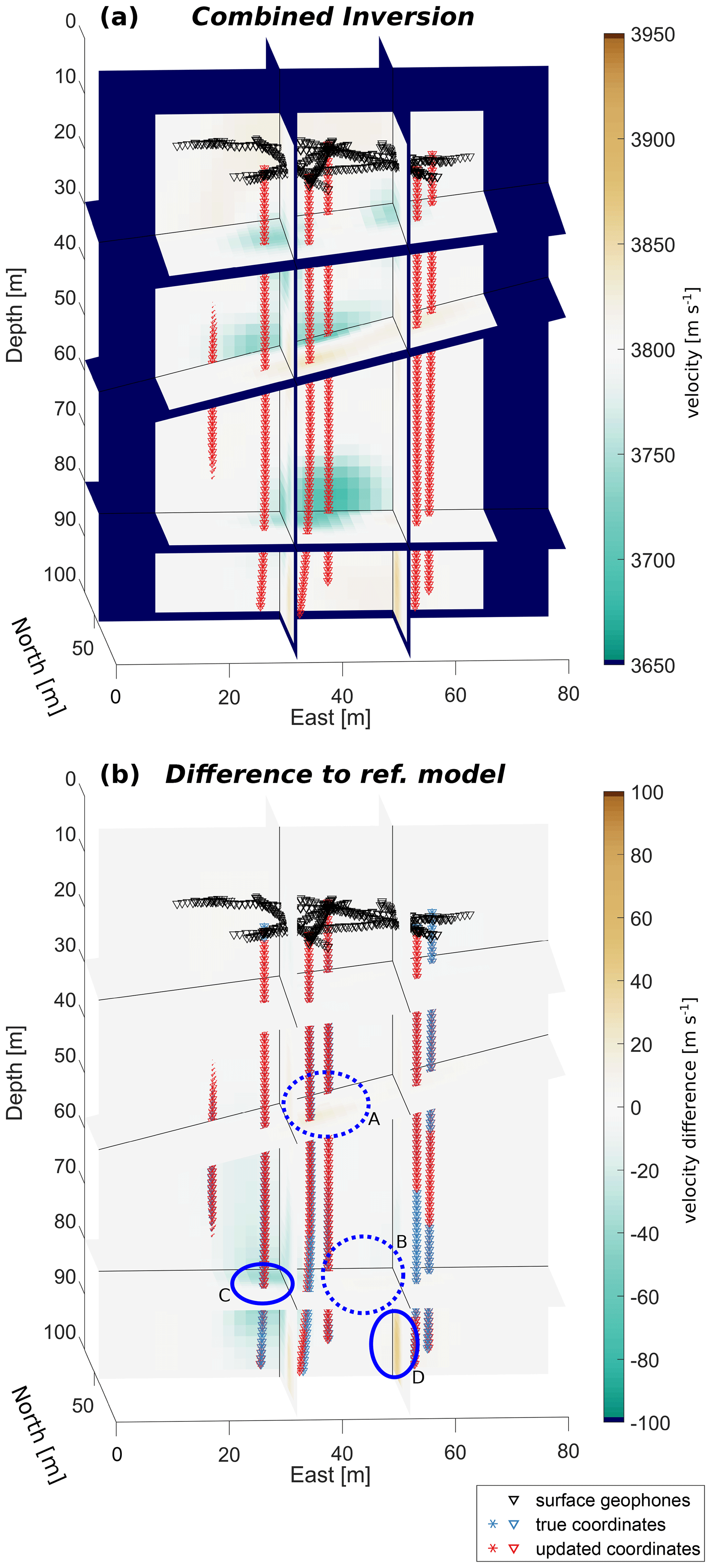
Figure 5 Results of the sequential (velocity and borehole trajectory) inversion with a synthetic example data set and initially straight borehole trajectories. (a) Inversion results after seven steps of iteration; (b) difference between inversion results in (a) and the reference model (Fig. 3a). Triangles and asterisks represent receiver and source positions.

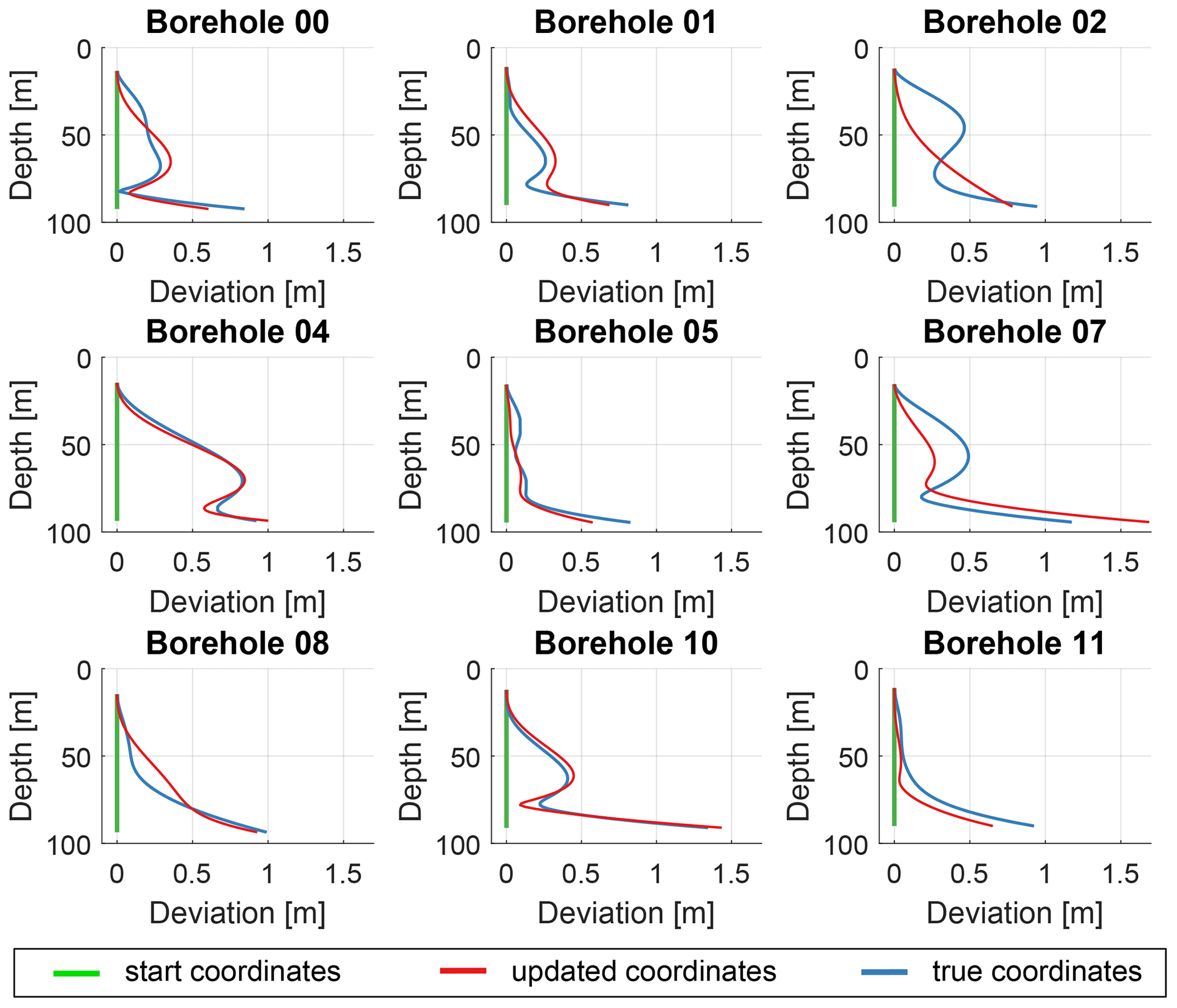
Figure 6 Deviations of the individual boreholes (locations shown in Fig. 1a) for the synthetic data set: start values for straight boreholes are plotted as green graphs, true borehole trajectories are shown as blue graphs, and the borehole deviations adjusted after seven iterations are plotted as red curves.

The borehole trajectories, obtained from the trajectory inversion, are shown in Fig. 6 and compared with initial (straight) and true trajectories. For some boreholes, the inverted borehole trajectory closely resembles the true borehole path. For other boreholes, e.g. borehole BH02 and BH07, the inversion algorithm did not fully converge towards the true solution. Instead, some minor artefacts are still visible in the velocity profile in the vicinity of these boreholes (for an enhanced three-dimensional view we refer to our “Video supplement”; Hellmann, 2022b). This is a trade-off that cannot fully be avoided by such a velocity–borehole inversion as both solutions provide similar residual errors. If a priori information about the magnitude of deformation or an initial guess for the main direction of deformation is available, this information could be used to avoid a start with straight vertical boreholes and provide further constraints for the individual boreholes. However, boreholes that are only part of a single two-dimensional profile cannot be fitted by our algorithm at all, as the degree of freedom is then higher than the geometric information obtained from such a two-dimensional seismic profile (e.g. dashed profile BH06–BH12 in Fig. 1a). In this case, we observed strong oscillations or large deviations of the trajectories perpendicular to the measurement plane.

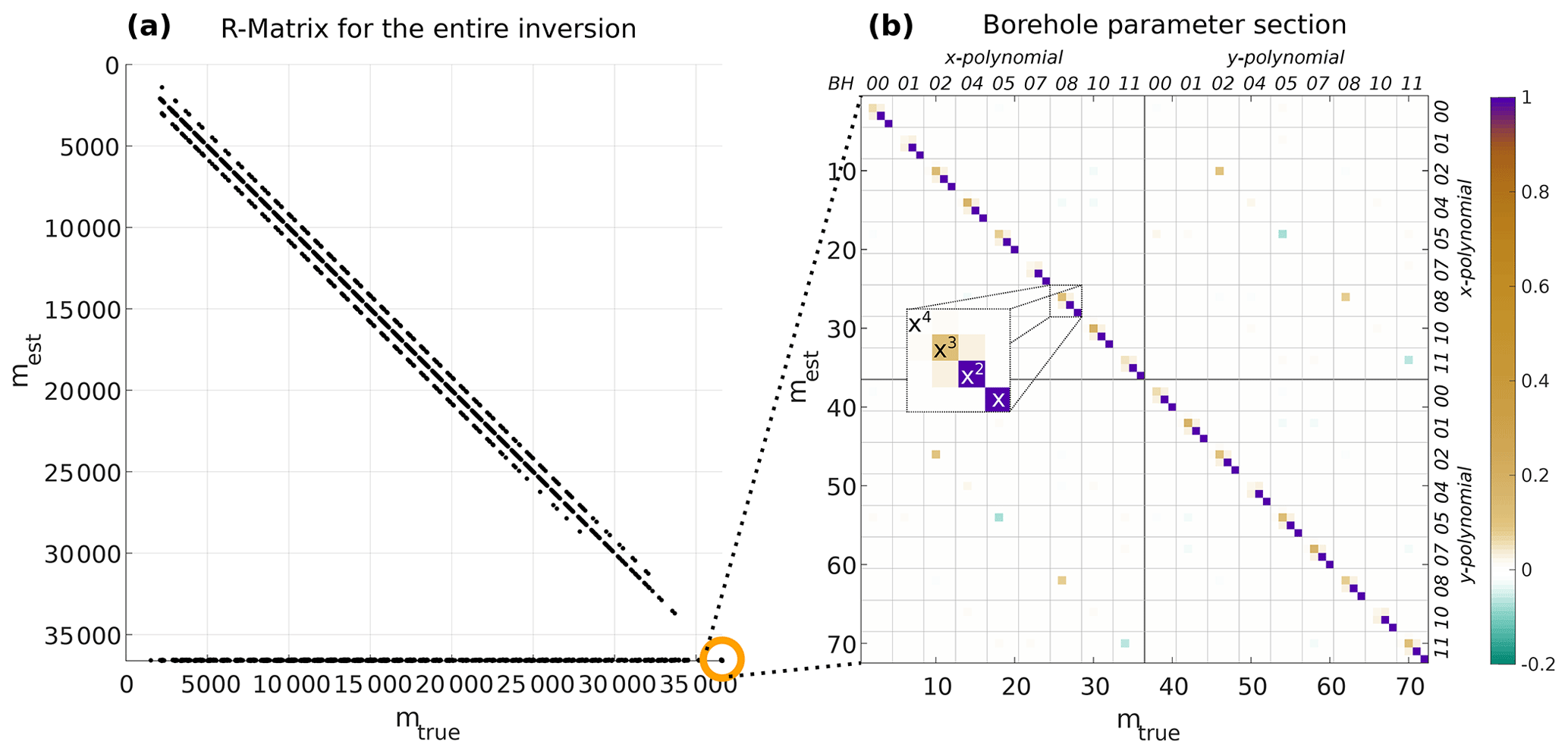
Figure 7 Resolution matrix for the coupled velocity and borehole trajectory inversion. (a) The entire matrix for all 36 612 model parameters; the 72 parameters of the borehole adjustments are highlighted in the orange circle. Only values of the matrix larger than 0.05 are shown as black dots. (b) Zoomed view of the borehole model parameters with colour-coded values. The excerpt illustrates the order of the four polynomial coefficients as an example.

The issue of resolving the individual model parameters can be further investigated with the resolution matrix R (e.g. Menke, 1984),

$$\begin{array}{}\text{(8)}& {\mathit{m}}^{\text{est}}=\mathbf{R}{\mathit{m}}^{\text{true}}\end{array}$$

that connects the true model parameter m^true with the estimated parameters m^est. The resolution matrix for our velocity-borehole inversion scheme is defined as

$$\begin{array}{}\text{(9)}& \begin{array}{rl}\mathbf{R}& ={\left({\left(\begin{array}{cc}\mathbf{G}& \mathbf{J}\\ {\mathbf{W}}_{\mathrm{M}}& \mathrm{0}\\ \mathrm{0}& {\mathbf{W}}_{\mathrm{J}}\end{array}\right)}^{\mathrm{T}}\left(\begin{array}{cc}\mathbf{G}& \mathbf{J}\\ {\mathbf{W}}_{\mathrm{M}}& \mathrm{0}\\ \mathrm{0}& {\mathbf{W}}_{\mathrm{J}}\end{array}\right)\right)}^{-\mathrm{1}}\\ & \times \left({\left(\begin{array}{cc}\mathbf{G}& \mathbf{J}\end{array}\right)}^{\mathrm{T}}\left(\begin{array}{cc}\mathbf{G}& \mathbf{J}\end{array}\right)\right),\end{array}\end{array}$$

where G is the sensitivity matrix (Jacobian matrix) for the velocity inversion, and J is the Jacobian matrix for the borehole inversion as defined in Eq. (5). The regularisation matrices (combining damping and smoothing) are given by W_M for the velocity inversion and by W_J for the borehole trajectory inversion, respectively. The resolution matrix for the synthetic example in Fig. 5b is shown in Fig. 7. Only values larger than 0.05 are plotted as black dots. The matrix has a tridiagonal structure with the highest values along its main diagonal. Therefore, the estimated model parameter is mainly dependent on its true value. However, for the velocity inversion parameters, this dependency is rather weak (all values are < 0.2). In addition, elements along two minor diagonals also influence the estimated parameters. These are the neighbouring model parameters along the ray path that also affect the velocity of the current cell.

For the borehole inversion parameters, the relationship between estimated and true parameters is much stronger, especially for the polynomial coefficients of degree 1 and 2. As shown in Fig. 7b, the third element and fourth element of each set of borehole coefficients representing degree 1 and 2 show high values > 0.99. Therefore, these coefficients are well resolved in the inversion. However, the higher-order polynomial coefficients (third and fourth degree) are also weakly resolved for the majority of the boreholes (small values for these coefficients in Fig. 7b). This indicates that the exact values for the coefficients cannot be determined independently and several solutions lead to similar results. The borehole coefficients of a particular borehole are also dependent on the coefficients of the other boreholes, and its higher-order coefficients are often accompanied by larger off-diagonal elements that indicate this dependency. Here, the most prominent off-diagonal elements that are visible in Fig. 7b are part of the other component of the borehole (i.e. the higher-order coefficients of the polynomial q(z) interfere with the coefficients of p(z)), indicating that the two polynomials are not fully linearly independent. This is not surprising, when considering the geometry of the experimental setup (Fig. 1a) that is based on field measurements with a limited number of source–receiver combinations. The data set for the three-dimensional inversion consists of a set of two-dimensional profiles covering the volume within the ring of boreholes. In this setup, each borehole is used as a source and receiver hole together with two other boreholes. Therefore, a minimisation of the error can be achieved by adjusting at least one of the polynomials of these boreholes relevant for the current set of measurements. This leads to a reduced azimuthal illumination of the borehole trajectories, and several equally good solutions for the borehole trajectories are possible that reduce the number of fully independent model parameters.

The resolution matrix is also a useful tool to investigate whether the model parameters of the velocity inversion also affect the borehole trajectory inversion and vice versa. If there is a dependency between these parameters we expect to see off-diagonal elements in the resolution matrix. As shown in Fig. 7a, off-diagonal elements appear in the lower-left corner of the matrix, but not in the upper-right part. This implies that the estimated borehole polynomials depend on the defined velocity parameters between the boreholes. This is not surprising since the velocity is included in the calculation of the sensitivities for the borehole inversion and has already been investigated by Maurer (1996). In contrast, there is no dependence of the velocity parameters on the selected coefficients of the borehole trajectories. Therefore, the velocity inversion can be obtained independently from the borehole parameters, and a separate borehole trajectory inversion is acceptable if the most recent results for the velocities are considered in the iteration step of the borehole inversion.

5 Application on field data

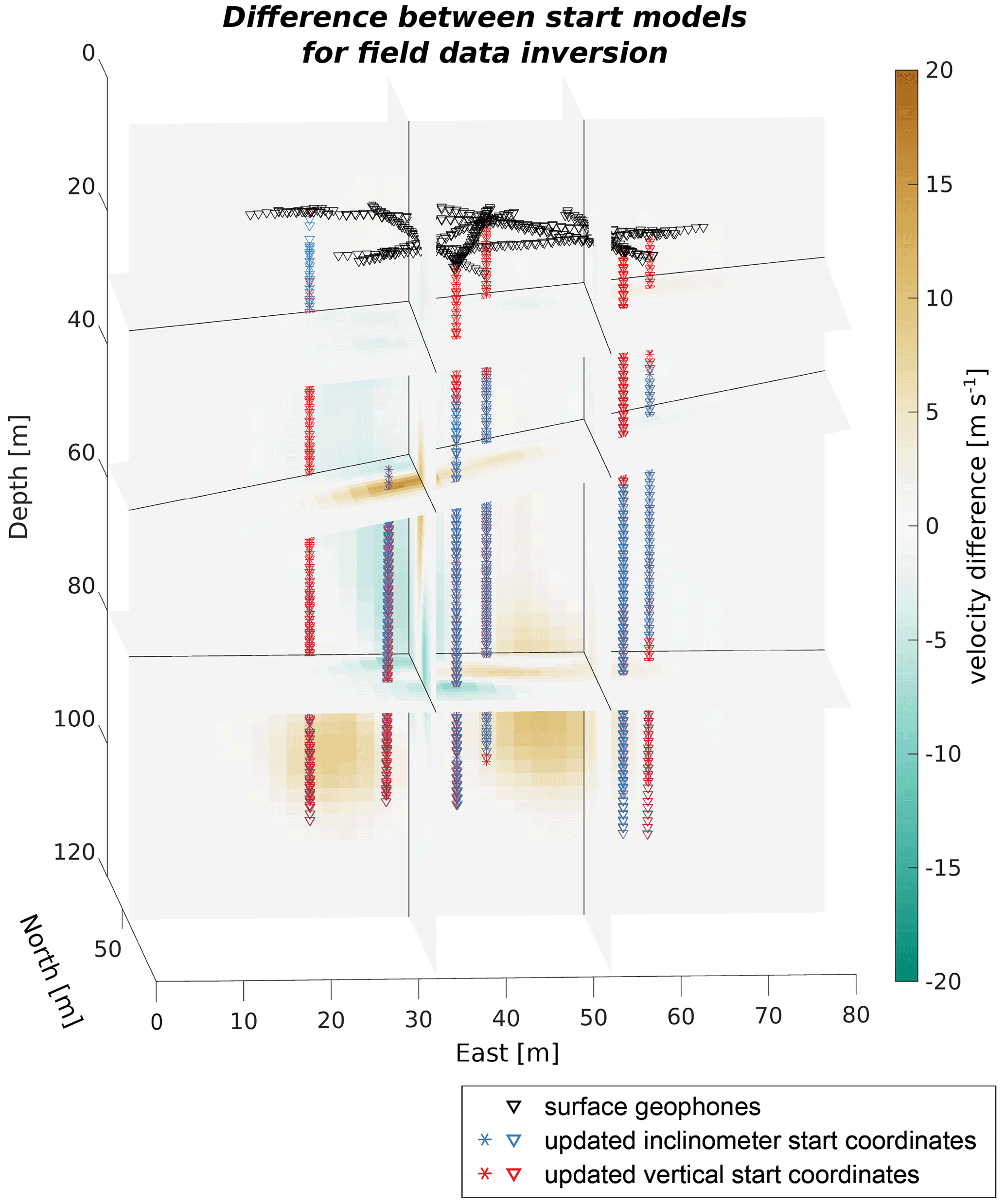
For the field data set, we determined the travel times of the recorded P waves with a cross-correlation algorithm between repetitive measurements (in general three repetitions) within a window with a length of up to 4 ms depending on the distance around the estimated arrival time. Afterwards, these absolute values of the picked travel times were compared. If they differed by fewer than three samples (or 60 µs) the median value of the arrival times was selected for the source–receiver pair. About 7.2 % (25 860 out of 359 369) of all source–receiver pairs had to be excluded from the analysis due to larger discrepancies. In a next step, we obtained a velocity inversion followed by a combined velocity and borehole inversion. The results for the velocity inversion are shown in Fig. 8a. Similar to our synthetic data, we locally observe very high velocities (yellow ellipses). We interpret them as artefacts since in previous experiments on ice core samples (Hellmann et al., 2021a) we observed a mean seismic velocity of 3820 m s⁻¹ in pure ice at −5 ^∘C with less than 2 % air bubbles. We are not expecting to reach such high values for in situ measurements due to the high amount of meltwater that is present in the entire glacier in summer. In addition, we also observe velocity artefacts at the lower end of several boreholes similar to those in our synthetic example. Therefore, we applied our borehole trajectory inversion scheme in addition to the velocity inversion. We considered two slightly different start models. The first one uses the trajectories derived from inclinometer measurements as start values. The results are shown in Fig. 8b. The second start model considers vertical boreholes. The differences between the two are discussed below and are rather small. Therefore, we did not include the results here but provide a difference plot in the Appendix (Fig. A1). The velocity and the two combined inversion models show a low-velocity zone close to the surface, which we interpret as a zone of weathered, water-saturated ice. The meltwater, generated at the surface of the glacier due to the positive energy flux into the ice, leads to a decrease in the seismic velocities. Between 15 and 70 m, we observe a rather homogeneous zone with a velocity of v = 3750 ± 30 m s⁻¹. These values lie in the range of values commonly observed in glacier ice (Deichmann et al., 2000; Walter et al., 2009; Church et al., 2019). Similarly, in the lower part of the glacier, an englacial drainage system, observed in the vicinity of our investigation area by Church et al. (2020, 2021), also results in larger amounts of water. Therefore, the velocity decreases again.

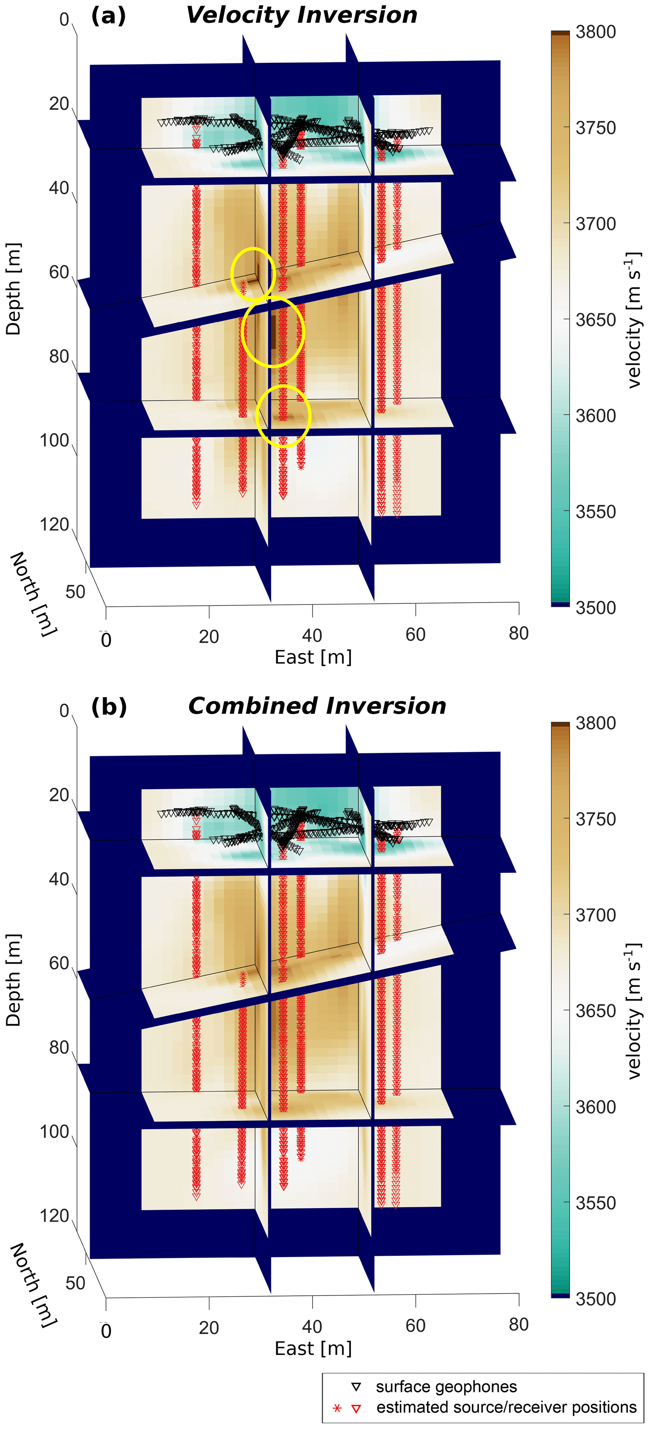
Figure 8 Inversion results for field data from Rhonegletscher. (a) Results from the velocity inversion (seven iterations) without adjustment of the boreholes (trajectories from inclinometer data). (b) Results from the combined velocity and borehole inversion with inclinometer-derived start trajectories. Yellow ellipses in (a) emphasise the areas with potential velocity artefacts.

Table 2 RMSEs for the velocity and the combined inversion applied to the field data.

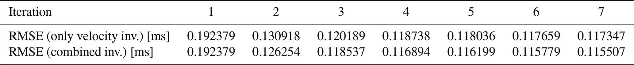
Table 3 Maximum degree of the two polynomials for each borehole.

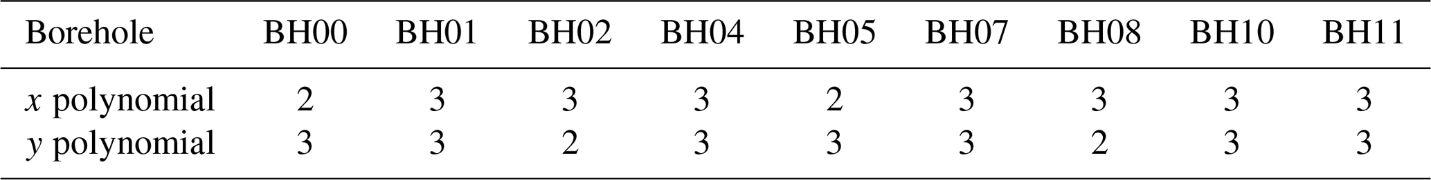
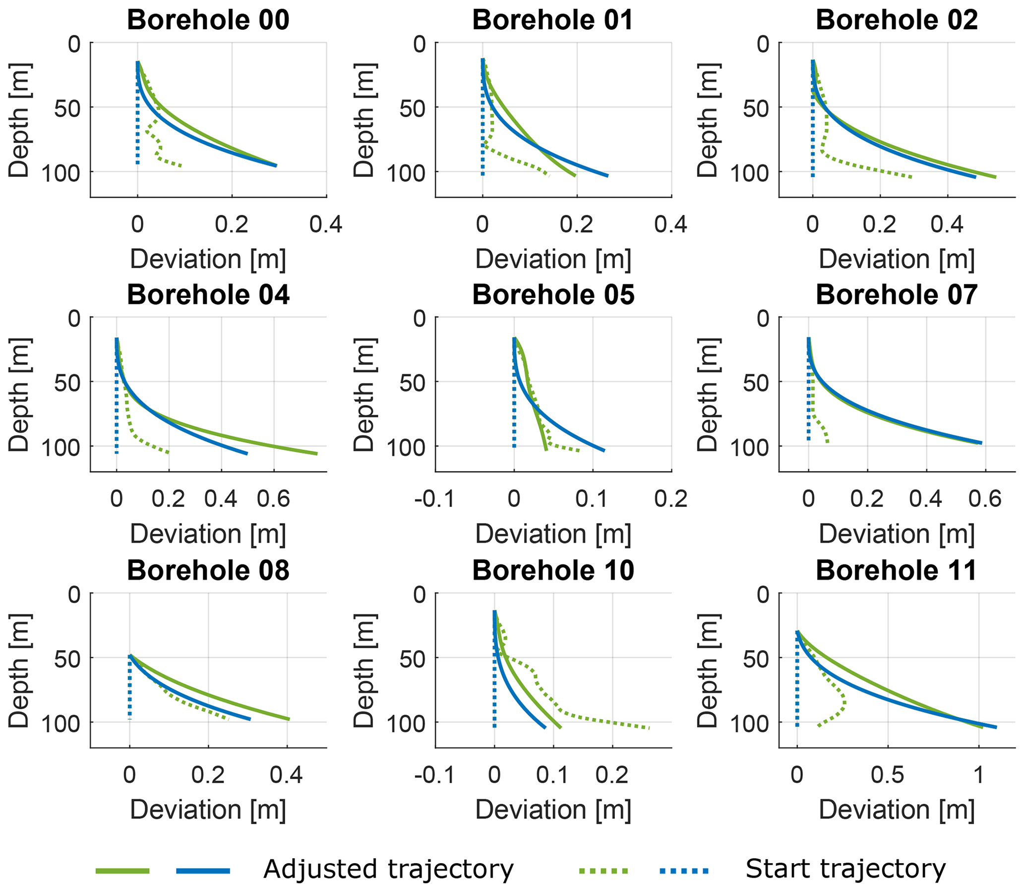
Figure 9 Results of borehole trajectory adjustment for field data. Green profiles show initial (dashed line) and final (solid line) borehole trajectories for a setup considering a priori inclinometer data; blue profiles show the borehole trajectories estimated from initially vertical (straight) boreholes.

The rms values of both inversion schemes are similar, as shown in Table 2. As a consequence, the velocity structure resulting form the two inversion schemes does not differ significantly. Nevertheless, velocity artefacts visible in the velocity inversion vanish in the combined inversion depending on the selected damping factor. This damping factor also affects how strongly the adjusted boreholes deviate from the initial guess. Values that are too high (damping factor ≥ 10 000) do not significantly change the borehole trajectories and the artefacts are still in place. A very low damping factor (< 1000) leads to unrealistically large adjustments with up to several metres at the bottom of the borehole. Therefore, we selected a damping factor that provided the best compromise between adjustment of boreholes and removing the velocity artefacts. Furthermore, we considered different start values for the trajectories to test the robustness of our algorithm. Keeping all other regularisation factors identical, we started with perfectly vertical boreholes and already inclined boreholes. The latter are interpolated trajectories (by means of time) derived from the repeated inclinometer measurements. Figure 8b shows the results for an inversion with borehole trajectories interpolated from inclinometer measurements. We also repeated the calculations for initially vertical borehole trajectories. The results are nearly identical within a range of 40 m s⁻¹ as shown in the difference plot in Fig. A1. In both cases, each borehole has been approximated by two mutually perpendicular polynomials. The degree of the individual polynomials is provided in Table 3. The resulting adjustments of the trajectories for both start models (starting with straight vertical borehole trajectories and trajectories derived from inclinometer measurements) are compared in Fig. 9. The trajectories are consistent, providing evidence that the algorithm provides robust results. This is especially useful if no a priori (i.e. inclinometer) measurements of the trajectories are available. In addition, the results for the majority of the boreholes are consistent with regard to the time difference between drilling and day of measurement. The boreholes BH02, BH04, BH08, and BH10 were occupied by the instruments about 20–23 d after drilling and show larger deviations compared to the holes BH01 and BH05, which were occupied 11–14 d after drilling. The ongoing ice flow causes a slightly enhanced deviation at a later stage.

Nevertheless, boreholes BH07 and BH11 show large deviations. Their maximum deviation at the bottom is 0.6 and 1 m, respectively, although the measurements were obtained just 11–14 d after drilling of the holes (together with BH01 and BH05). Glacier flow rates of 0.06 m d⁻¹ on average measured at the glacier surface during the summer period imply that this deviation could not be caused by the ice flow when considering a typical parabolic decrease in the flow rate with depth. Furthermore, the inclinometer measurements do not provide any hint of such strong deviations. Therefore, we expect that measurement errors such as picking errors are compensated for through overly adjusted borehole trajectories during the inversion. Further evidence of this assumption is given by the fact that BH11 was only used as a source hole and only partially as receiver hole (along a profile to BH07 but not to BH05), since it drained just after the second out of 3 d of measurements. Therefore, the number of data points in this borehole is much lower and, thus the capability of our algorithm decreases due to poor constraints by the data. Since BH07 is directly connected to BH11 with two reciprocal profiles, errors in the trajectory of BH11 may also affect BH07 and would explain the still quite large deviations.

In summary, our inversion algorithm provides the option to adjust borehole trajectories such that artefacts in the velocity inversion can be removed. For a good three-dimensional adjustment, a reasonably high number of data points along these trajectories for different directions is required. For our specific experimental setup on a continuously moving glacier, this inversion scheme provides improved results.

6 Discussion

The combined inversion scheme provides the advantage of a subsequent correction for the borehole coordinates if no or limited information about the positions of sources and receivers is available. However, there is a risk that the coordinate adjustment will suppress the appearance of real velocity anomalies in the tomogram. We avoid this by decoupling the two parts of the inverse algorithm. Furthermore, an additional check of whether the new coordinates reduce the RMSE of the entire data set was implemented. This led to a more cautious adjustment. For our field data set, only two to three coordinate adjustments in the first iterations were required. Afterwards, the inversion continued with a traditional velocity inversion and explained the rather similar rms values observed in Table 2. This is the major advantage of the sequential inversion scheme with two independent inversion branches compared to an “all-in-one” inversion. Nevertheless, the borehole trajectory inversion still relies on a priori knowledge such as inclinometer estimates and must be tuned accordingly to find the best solution for this equifinality problem.

6.1 Comparison with previous studies

The idea for a sequential inversion scheme is mainly driven by the findings described in Maurer (1996) and following projects in the research group. Two-dimensional analyses are usually easier to evaluate as the degree of freedom is lower than in a three-dimensional setting. However, as Irving et al. (2007) already described in detail, off-plane effects may lead to misinterpretations of the resulting data. Especially when analysing an azimuthally dependent variation in the seismic velocities (for example, due to changes in the ice crystal orientation relative to the glacier flow), those off-plane effects have to be avoided. Cheng et al. (2016) described a similar three-dimensional issue when trying to detect boulders in the subsurface. With their numerical modellings, they presented the advantages of the three-dimensional algorithms with the resulting higher capability. Due to these advantages of three-dimensional approaches, we considered them here as well.

Next to the issues in the velocity model, we also have to consider the ice flow and thus a changing geometry setup when obtaining the inversion. Once again, some successful concepts were described in earlier studies. As an example, Bergman et al. (2004) presented their results for a layered subsurface. They applied some static corrections to account for the layers and changes in between. Although glaciers may also have some ice layers, such as air-bubble-free and air-bubble-rich layers (Hubbard et al., 2008), the current study is mainly driven by issues due to the glacier flow itself and the consecutive deformation of the initially rather straight boreholes in the glacier. Therefore, we could not consider such an approach for our data analysis. In one of the most recent publications, Fernandes and Mosegaard (2022) provided a promising statistical concept in which they determine the probability of the borehole positions along a given trajectory by perturbating the model parameters. This might be another promising approach that we did not consider. However, there might be some issues due either to a very large number of sources and receivers or a poorly constrained initial borehole trajectory that even further deforms over time. As an alternative, we considered the methodology described by Maurer and Green (1997). They analysed the effect of coordinate mislocations on cross-hole tomography results in 2D. Their findings were similar to our observations after data acquisition and processing. We therefore considered their concept and transferred it into 3D.

6.2 Interference of the borehole inversion scheme with velocity anisotropy

An adjustment of the borehole coordinates provides the opportunity to account for deformations of the boreholes due to a movement of the subsurface. This adjustment is based on the current velocity model as it considers the mean velocity between the source and receiver. However, other physical quantities such as seismic anisotropy may introduce apparent errors in this seismic velocity values. In glaciers, macrostructural features, such as the crevasses or englacial channels used in our synthetic data set, may cause velocity anisotropy in the seismic data. Besides this macrostructure, there is the crystal orientation fabric that can also introduce such anisotropy. This anisotropy appears since the seismic velocity in a single ice crystal depends on the propagation direction of the seismic wave relative to the c axis of the crystal. When the ice crystals in a polycrystalline glacier are oriented in a preferred direction relative to given stress conditions, a seismic wave travels parallel to this alignment of the c axes with a higher velocity compared to other directions. This COF-derived seismic anisotropy has been investigated in several previous studies (Blankenship and Bentley, 1987; Diez et al., 2015; Kerch et al., 2018). When not considering this velocity anisotropy effect, a borehole coordinate adjustment scheme could at least partially compensate for this effect.

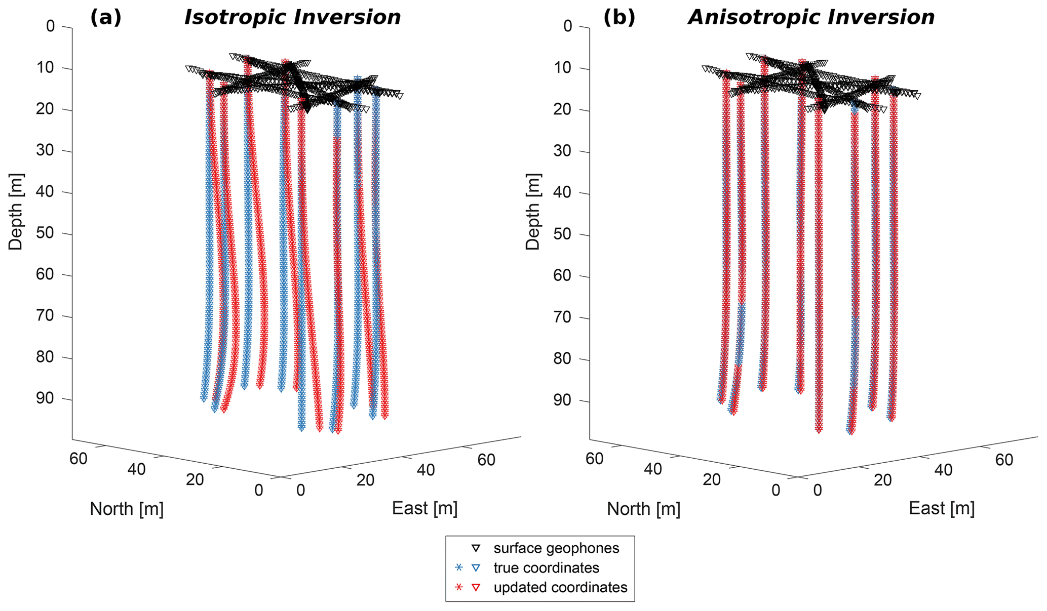
Figure 10 Borehole trajectories for different inversion schemes: (a) results for the coordinates from a combined velocity and borehole inversion without consideration of anisotropy. (b) Results for the coordinates from a combined inversion with borehole polynomials of degree x³ that additionally inverts for the four anisotropy parameters. Triangles and asterisks represent receiver and source positions.

If significant velocity anisotropy is present, this could lead to flawed adjustments of the borehole trajectories, which in turn, reduce or entirely remove the anisotropy effect. We have investigated this issue with a synthetic data set. The geometric setup consists of eight straight boreholes (BH01, BH02, BH04, BH05, BH07, BH08, BH10, and BH11 in Fig. 1a), and each source hole is again connected to two receiver holes on opposite sides of the ring as in the previous calculations. The true velocity model is set to a homogeneous velocity value of 3800 m s⁻¹ with an additional ellipsoidal anisotropy of 10 % ($\mathit{\delta }=\mathit{ϵ}=\mathrm{0.1}$) according to the definitions of Thomsen (1986). The azimuthal direction of maximum anisotropy was chosen to be ϑ_a = 160^∘ with a slightly downwards-pointing inclination of φ_a = −15^∘. The anisotropy effect was added to the modelled travel times by adding a time shift depending on the angle between maximum anisotropy (ϑ_a,φ_a) and the wavefront (derived from the given ray path as defined in Thomsen, 1986). In a first run, we used our combined velocity and borehole inversion scheme to invert for such an anisotropic model starting with vertical boreholes. The resulting borehole trajectories, shown in Fig. 10a, incorporate the anisotropy effect up to a certain degree and drift away from the true trajectories. We then extended our borehole inversion with four additional model parameters for the anisotropy parameters and defined a set of estimated values close to but slightly below the true values (i.e. $\mathit{\delta }=\mathit{ϵ}=\mathrm{0.05}$, ϑ_a = 180^∘, and φ_a = 0^∘). The sensitivities for the four Thomsen parameters were calculated numerically: that is,

$$\begin{array}{}\text{(10)}& {\displaystyle \frac{\partial t}{\partial m_i}}={\displaystyle \frac{f(m_i+\mathrm{\Delta }{m}_i)-f\left(m_i\right)}{\mathrm{\Delta }{m}_i}},\end{array}$$

with initial estimates for the four parameters $\mathit{m}=(\mathit{\delta },\mathit{ϵ},{\mathit{\vartheta }}_{\mathrm{a}}$, and φ_a) as well as a small perturbation Δm for each value. f(m_i) and f(m_i+Δm_i) are results for the calculated travel times when considering the estimated and perturbed anisotropy parameters, respectively. When applying this extended inversion algorithm to a data set with the correct values for the isotropic velocity and borehole trajectories, the true anisotropy parameters could be obtained within a few iteration steps. However, when again considering straight boreholes to be start trajectories, the tests provide evidence that anisotropy parameters are still highly dependent on the estimated borehole parameters. The corresponding areas in the resolution matrix for such an experimental setup (Fig. 11) are occupied by large values that indicate a dependency between these model parameters. In addition, Fig. 11 also shows that these model parameters, in particular of the borehole trajectories that represent the higher-order polynomials, significantly interfere with the anisotropy values. In particular, the azimuthal angle of anisotropy interferes with the higher-order coefficients of all boreholes. This implies that the anisotropy can be erroneously caught by an adjustment of the borehole trajectories. In our synthetic example, this interaction manifests itself in very small adjustments of the anisotropy parameters when the degree of the polynomials is large enough. We observe this effect when considering polynomials of degree x⁴ or higher. In contrast, polynomials of degree x³ or lower determine almost correct values (< 0.01 for δ and ϵ; < 1.5^∘ for the angles) for the anisotropy parameters. However, smaller-order polynomials only provide a limited degree of freedom in order to explain deviations along the trajectories. For our synthetic data set, polynomials of degree x³ show optimal results for a simultaneous adjustment of anisotropy and borehole trajectories. Figure 10b shows the results of such an anisotropic inversion with a good fit between estimated and true borehole trajectories. We repeated these experiments with different deviations of the borehole trajectories and a range of initial values for the anisotropy parameters. All calculations lead to the same result, providing evidence that polynomials of degree x³ provide the best estimates. Higher-order polynomials incorporate the anisotropy into the trajectories and the anisotropy parameters are hardly adjusted. In turn, smaller-order polynomials suffer from a lower degree of freedom as mentioned above. As a conclusion, these observations confirm that anisotropy and borehole adjustment interfere with each other, and the inversion parameters must be selected in such a way that anisotropy that might be present in the analysed data set is not accidentally factored out by borehole adjustments.

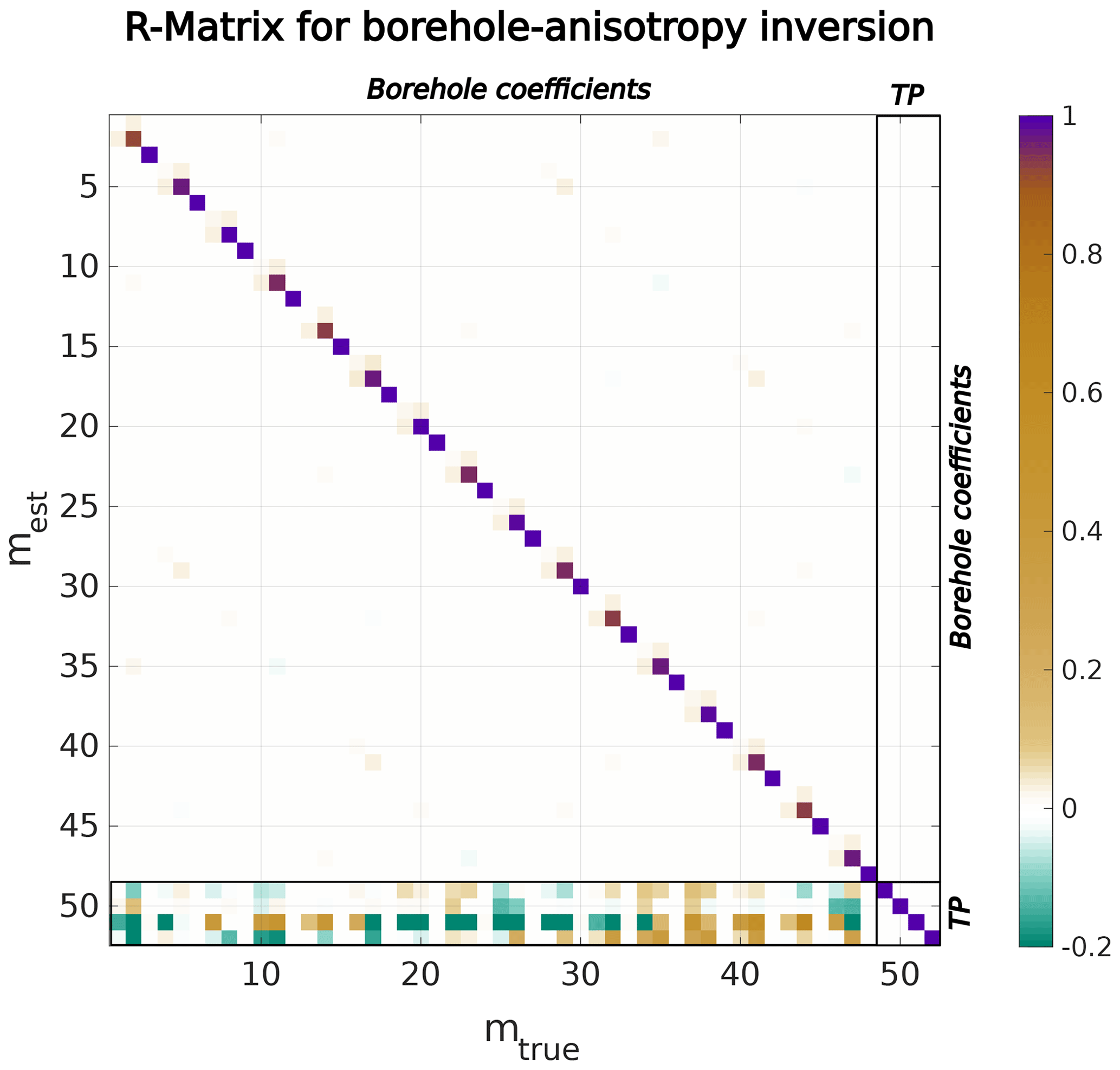
Figure 11 Resolution matrix for a combined inversion for borehole trajectories (third-order polynomials) and four anisotropy parameters (marked with TP for Thomsen parameters). The colours show the dependence of the true model parameter on estimated values. Off-diagonal values indicate interference between different model parameters. The four sectors provide an enhanced overview to distinguish between borehole coefficients and Thomsen parameters.

An application to our field data is difficult to assess since the azimuth and inclination of the COF vary with depth as described in our previous study: Hellmann et al. (2021b). Therefore, it was not possible to define a set of Thomsen parameters that describe the seismic velocity anisotropy derived for the COF of the entire ice column. Potentially, cross-hole experiments in polar ice with a rather constant COF, which allow for a definition of a set of Thomsen parameters for larger parts of the ice column, are recommended here for further investigations.

7 Conclusions

In this paper, we presented a mathematically simple but efficient approach for a combined velocity and borehole trajectory inversion. This inversion scheme is especially useful for measurements in a deforming subsurface such as experiments in alpine glaciers or ice sheets. The inversion process consists of a typical three-dimensional velocity inversion and an additional borehole trajectory adjustment. All sources and receivers in each borehole are summarised along a trajectory that is characterised by two orthogonal polynomials. The two steps for velocity and borehole inversion are decoupled as shown by the resolution matrix, and thus we only consider further adjustments of the borehole trajectories if this reduces the entire RMSE of the system. With this sequential inversion, we could significantly reduce velocity artefacts that are a result of poorly determined source and receiver positions.

The adjustments are plausible for our field data, but we have also shown that poorly constrained boreholes, e.g. a small number of sources and receivers along the borehole, may lead to larger deviations and potentially to an overfitting of noise and picking errors. Therefore, a data-set-dependent damping factor, which considers a priori information, is required. A weakness of our inversion methodology includes the somewhat subjective choice of the regularisation parameters. In future investigations, this may be improved in two ways. When more advanced information on the glacier movements is available, this could be supplied in the form of further constraints to the inversion problem. Alternatively, the various regularisation parameters could be determined in a more systematic fashion (compared with our trial-and-error approach). A possible option may include generalised cross-validation (e.g. Golub et al., 1979) or similar techniques. In addition, the algorithm only works for a set of profiles with different azimuths and cannot successfully be applied to two-dimensional profiles. In this case, the polynomial coefficients cannot be determined, and oscillations or large deviations occur at the bottom of the boreholes. Nevertheless, we could also show that the coupled scheme is rather robust and converges against very similar solutions for different start coordinates for a reasonably well-constrained inversion problem. We also judge that this approach can be easily applied to other cross-borehole experiments or VSP experiments on solid ground with poorly constrained borehole trajectories. In addition, this approach can in principle be applied to any geophysical borehole experiment beyond seismic investigations. However, its effectiveness needs to be individually studied and validated.

We have also analysed the interdependence between anisotropy and borehole trajectory adjustments. Excessive corrections of the borehole trajectories can at least partially compensate for the inherent velocity anisotropy. A higher degree of freedom (or flexibility) in the borehole parameters (that is, the use of higher-order polynomials) leads to a compensation for any weak ellipsoidal anisotropy. Therefore, it is highly recommended to precisely determine the borehole trajectories during data acquisition. If there is no such a priori information available, the inversion parameters must be selected accordingly to avoid this issue. We have shown that a polynomial degree of x³ provides a good compromise between flexibility to account for changes along the trajectories and an overcompensation due to existing velocity anisotropy.

Appendix A

Figure A1 Velocity and coordinate differences for the field data for the combined inversions of the two start models with initially inclined boreholes (shown in Fig. 8b, blue asterisks and triangles) and initially fully vertical boreholes (red asterisks and triangles).