Global seismic energy scaling relationships based on the type of faulting

We derived scaling relationships for different seismic energy metrics for earthquakes around the globe with M_W > 6.0 from 1990 to 2022. The seismic energy estimations were derived with two methodologies, the first based on the velocity flux integration and the second based on finite-fault models. In the first case, we analyzed 3331 reported seismic energies derived by integrating far-field waveforms. In the latter methodology, we used the total moment rate functions and the approximation of the overdamped dynamics to quantify seismic energy from 231 finite-fault models (E_mrt and E_O, E_U, respectively). Both methodologies provide compatible energy estimates. The radiated seismic energies estimated from the slip models and integration of velocity records are also compared for different types of focal mechanisms (R, reverse; R-SS, reverse–strike-slip; SS, strike-slip; SS-R, strike-slip–reverse; SS-N, strike-slip–normal; N, normal; and N-SS, normal–strike-slip), and then used to derive converting scaling relations among the different energy types. Additionally, the behavior of radiated seismic energy (E_R), energy-to-moment ratio ($E_{\mathrm{R}}/M_{\mathrm{0}}$), and apparent stress (τ_α) for different rupture types at a global scale is examined by considering depth variations in mechanical properties, such as seismic velocities, rock densities, and rigidities. For this purpose, we used a 1-D global velocity model. The $E_{\mathrm{R}}/M_{\mathrm{0}}$ ratio is, based on statistical t tests, largest for strike-slip earthquakes, followed by normal-faulting events, with the lowest values for reverse earthquakes for hypocentral depths < 90 km. Not enough data are available for statistical tests at deeper intervals except for the 90 to 120 km range, where we can satisfactorily conclude that $E_{\mathrm{R}}/M_{\mathrm{0}}$ for R-SS and SS-R types is larger than for N-type faulting, which also conforms to the previous assumption. In agreement with previous studies, our results exhibit a robust variation in τ_α with the focal mechanism. Regarding the behavior of τ_α with depth, our results agree with the existence of a bimodal distribution with two depth intervals where the apparent stress is maximum for normal-faulting earthquakes. At depths in the range of 180–240 km, τ_α for reverse earthquakes is higher than for normal-faulting events. We find the trend E_U > E_mrt > E_O for all mechanism types based on statistical t tests. Finite-fault energy estimations also support focal mechanism dependence of apparent stress but only for shallow earthquakes (Z < 30 km). The slip distribution population used was too small to conclude that finite-fault energy estimations support the dependence of average apparent stress on rupture type at different depth intervals.

1 Introduction

The radiated seismic energy (E_R) is a crucial source parameter that accounts for the size of an earthquake. The seismic energy is also a valuable parameter for understanding the dynamics of the rupture, especially in the case of large and complex earthquake sources (Venkataraman and Kanamori, 2004a; Convers and Newman, 2011). The radiated seismic energy is considered the main contribution to the total seismic energy during the failure process (the sum of radiated energy, fracture energy, and thermal energy) (Boatwright and Choy, 1986). The most common approach to calculating E_R requires the integration of radiated energy flux in velocity-squared seismograms (Haskell, 1964; Thatcher and Hanks, 1973; Boatwright, 1980; Kanamori et al., 1993; Boatwright and Choy, 1986; Singh and Ordaz, 1994; Choy and Boatwright, 1995; Pérez-Campos and Beroza, 2001). In order to recover the E_R of an event, the seismic records have to be corrected for propagation path and source effects such as attenuation, site effects, geometric spreading, radiation pattern, and directivity. Information on the Earth's structure is required to calculate seismic energy since E_R needs to be measured over a broad range of distances. Inaccurate information on the Earth's structure results in uncertainties in energy estimations, particularly at higher frequencies (Venkataraman and Kanamori, 2004a). Furthermore, previous studies showed that estimates of E_R based on regional and teleseismic data might differ by as much as a factor of 10 for the same earthquake (Singh and Ordaz, 1994).

Choy and Boatwright (1995) reported a focal mechanism dependence of E_R. Later, this observation was confirmed by Pérez-Campos and Beroza (2001), but they showed that the mechanism dependence is not as strong as reported previously. The degree of dependence of seismic energy on the focal mechanism is affected by several factors that bias the estimate (e.g., uncertainties in the corner frequency, geometrical spreading, hypocentral depth, and focal mechanism) (Pérez-Campos and Beroza, 2001). This dependence can be expressed in terms of the apparent stress (${\mathit{\tau }}_{\mathit{\alpha }}=\mathit{\mu }{E}_{\mathrm{R}}/M_{\mathrm{0}}$, where μ is the rigidity; Wyss and Brune, 1968), energy-to-moment ratio ($E_{\mathrm{R}}/M_{\mathrm{0}}$), or slowness parameter (Θ = ${\text{log}}_{\mathrm{10}}(E_{\mathrm{R}}/M_{\mathrm{0}}$); Newman and Okal, 1998). Previous studies showed that strike-slip events have the highest apparent stress (τ_α = 0.70 MPa), followed by normal-faulting and thrust earthquakes with 0.25 and 0.15 MPa, respectively (Pérez-Campos and Beroza, 2001). On the other hand, some authors have observed that the $E_{\mathrm{R}}/M_{\mathrm{0}}$ ratio is different for different types of earthquakes, particularly in subduction zones. For example, tsunami earthquakes have the smallest $E_{\mathrm{R}}/M_{\mathrm{0}}$ ratio (7 × 10⁻⁷ to 3 × 10⁻⁶), interplate and downdip events have a slightly larger ratio (5 × 10⁻⁶ to 2 × 10⁻⁵), and intraplate and deep earthquakes have $E_{\mathrm{R}}/M_{\mathrm{0}}$ ratios similar to crustal earthquakes (2 × 10⁻⁵ to 3 × 10⁻⁴) (Venkataraman and Kanamori, 2004a). The origin of the focal mechanism dependence is unclear, but it has been proposed that the stress drop is the cause of this dependence of the radiated seismic energy on the type of faulting (Pérez-Campos and Beroza, 2001).

Other approaches have also been used to calculate seismic energy, such as those based on finite-fault models (Ide, 2002; Venkataraman and Kanamori, 2004b; Senatorski, 2014). Ide (2002) calculated the radiated energy using an expression based on slip and stress on the fault plane. Energy estimates from this method tend to be smaller by about a factor of 3 compared with the integrating far-field waveforms method. Venkataraman and Kanamori (2004b) used a formula for the energy radiated seismically from a finite source as a function of the time-dependent seismic moment M₀(t) and the properties of the medium. Here, the moment rate function derived from kinematic inversion is used to calculate the E_R. On the other hand, Senatorski (2014) used an overdamped dynamics approximation for estimating the radiated seismic energy. The accuracy of this method depends on the rupture history. This approach provides two energy parameters: (1) the finite-fault overdamped dynamics approximation (E_O) and (2) the energy obtained from the averaged finite-fault model (E_U). In both cases, the seismic energy depends on the slip, rupture time, and seismic moment. According to Senatorski (2014), in most cases, the radiated seismic energy estimated by integrating digital seismic waveforms (E_R) is in the following range: E_U < E_R < E_O. Several seismic energy observations have been calculated and compiled in catalogs in the last 2 decades. In this study, we reexamine the possible dependence of seismic energy on the focal mechanism with an additional classification based on the type of rupture, considering pure and oblique mechanisms separately. We also investigate the potential influence of focal mechanisms on the derived estimates of radiated seismic energy from finite-fault models. Additionally, we explored the relationship between depth and the variables $E_{\mathrm{R}}/M_{\mathrm{0}}$ and τ_α. Furthermore, we established conversion relationships between various types of energy estimates. These findings play a crucial role in enhancing our understanding of the rupture processes associated with different types of earthquakes.

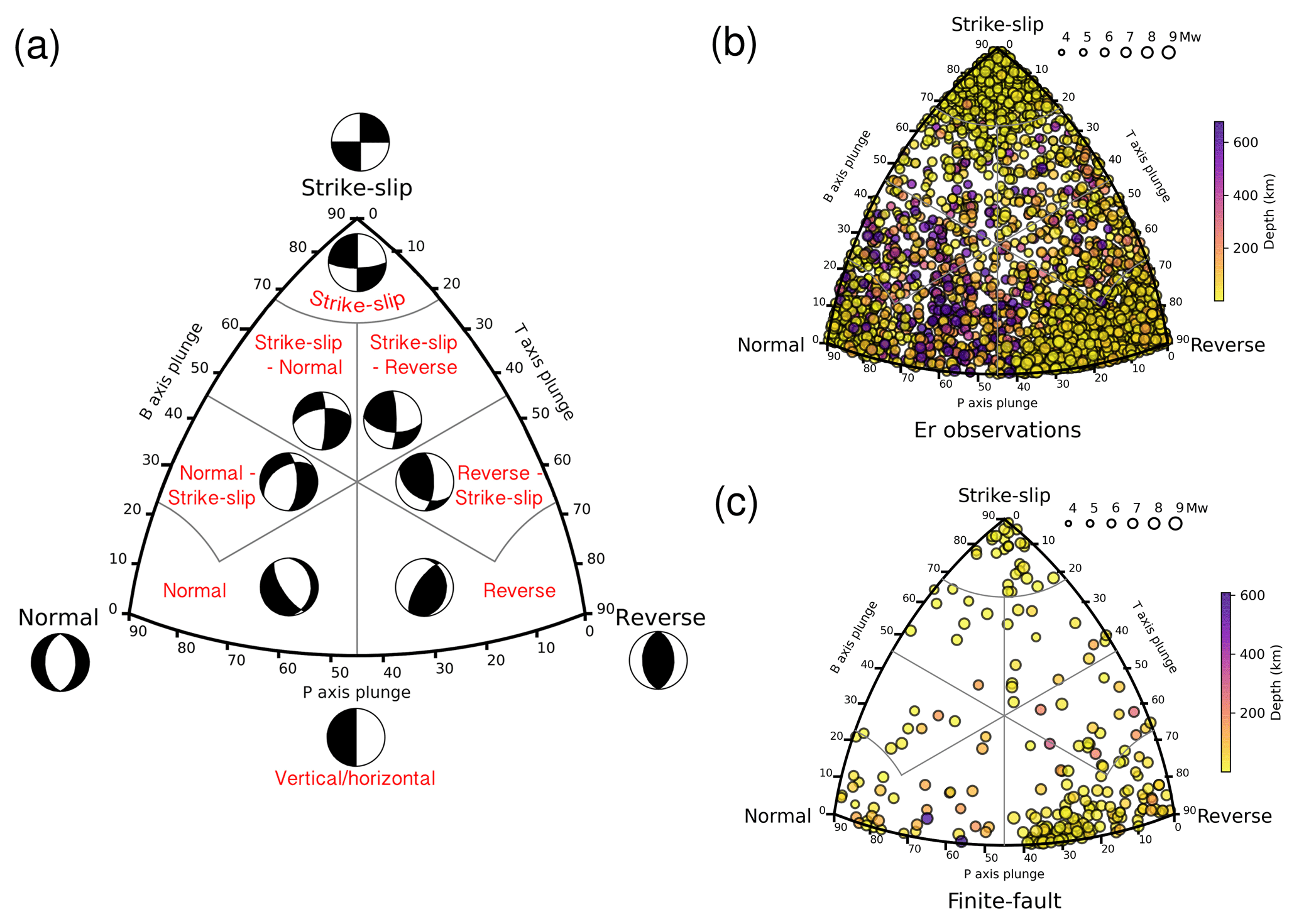
Figure 1 The Kaverina fault classification ternary diagram used to classify focal mechanisms (a). Focal mechanisms are denoted by circles filled to indicate event depth in kilometers, and the size of the circle indicates the moment magnitude of the earthquake (right panels). Panel (b) shows the rupture type of seismic events with a radiated seismic energy estimation. Rupture type of seismic events with a finite-fault model used to estimate the radiated energy (c).

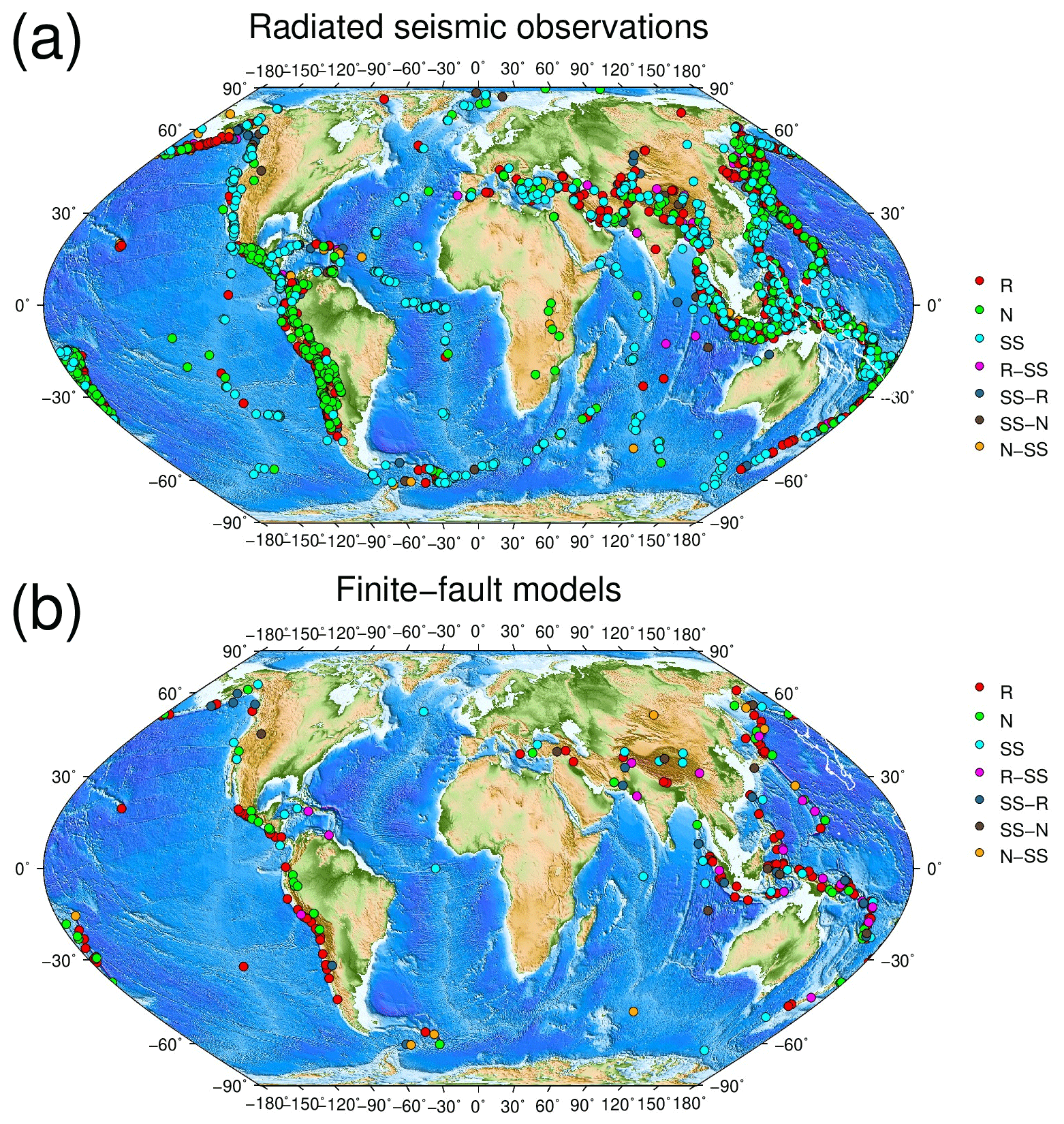
Figure 2 Hypocenter location and rupture type classification of earthquakes with reported radiated seismic energy (E_R) (a). Hypocenter location and rupture type classification of earthquakes with a finite-fault model used to calculate the radiated seismic energy (E_R) (b). R, reverse; R-SS, reverse–strike-slip; SS, strike-slip; SS-R, strike-slip–reverse; SS-N, strike-slip–normal; N, normal; and N-SS, normal–strike-slip.

2 Data and methods

2.1 Data

We retrieved and classified focal mechanism solutions from the Global Centroid Moment Tensor catalog (gCMT) (Dziewonski et al., 1981; Ekström et al., 2012) using a ternary diagram based on the Kaverina et al. (1996) projection. This approximation classifies focal mechanism into seven classes of earthquakes: (1) normal (N), (2) normal–strike-slip (N-SS), (3) strike-slip–normal (SS-N), (4) strike-slip (SS), (5) strike-slip–reverse (SS-R), (6) reverse–strike-slip (R-SS), and (7) reverse (R) (Fig. 1). For implementing fault-plane classification, we used the software FMC developed by Álvarez-Gómez (2019). Additionally, we used radiated seismic energy data and finite-fault models reported by the Incorporated Research Institutions for Seismology (IRIS) and the United States Geological Survey (USGS), respectively. To have homogeneity in the analyzed data, we did not include seismic energy observations and finite-fault models from other sources to avoid bias. IRIS reported automated E_R solutions for global earthquakes with an initial magnitude above M_W 6.0. We studied 3331 events worldwide during the period April 1990 to October 2022 (Fig. 2). Results include broadband energy solution (frequency band in the interval of 0.5–70 s) from vertical-component seismograms recorded at teleseismic distances (25^∘ $\le \mathrm{\Delta }\le$ 80^∘) (Convers and Newman, 2011; Hutko et al., 2017). Finite-fault models are determined with a kinematic inversion based on the wavelet domain (Ji et al., 2002). The procedure jointly inverts body and surface waves on a fault plane aligned with focal mechanism estimates from USGS W-phase or gCMT solutions. We used 231 finite-fault models from 1990 to 2022 (Fig. 2). After classifying the events, we determined scaling relationships for the reported seismic energies and analyzed the behavior of the $E_{\mathrm{R}}/M_{\mathrm{0}}$ ratio and τ_α. The seismic energy was also determined using finite-fault models with the techniques described in the following section to ascertain if there is a difference in estimates related to the faulting type. Seismic velocities and rock densities were taken from the ak135-F velocity model (Kennett et al., 1995; Montagner and Kennett, 1995); rigidity was calculated as μ=ρβ².

2.2 Methods

2.2.1 Radiated seismic energy derived from seismic waves

In the following, we describe the procedure used to calculate E_R implemented by IRIS and used as input to calculate apparent stress, energy-to-moment, and scaling relationships. Reported radiated seismic energies from IRIS were calculated with the method of Boatwright and Choy (1986) implemented by Convers and Newman (2011). Using velocity seismograms of the P-wave group (consisting of $P+\mathrm{pP}+\mathrm{sP}$ phases), the energy is calculated at teleseismic distances. The seismic energy flux from the P-wave group (ε_gP) is calculated from the velocity spectrum ($\left(\dot{u}\right(\mathit{\omega }\left)\right)$ as

$$\begin{array}{}\text{(1)}& {\mathit{\epsilon }}_{\mathrm{gP}}={\displaystyle \frac{\mathit{\rho }\left(z\right)\mathit{\alpha }\left(z\right)}{\mathit{\pi }}}\underset{\mathrm{0}}{\overset{\mathrm{\infty }}{\int }}\mathrm{|}\dot{u}\left(\mathit{\omega }\right){\mathrm{|}}^{\mathrm{2}}\text{exp}\left(\mathit{\omega }{t}_{\mathit{\alpha }}^{\ast }\right)\mathrm{d}\mathit{\omega },\end{array}$$

where ρ(z) and α(z) are the density and P-wave velocity at the source depth (z) and the exponential term $t_{\mathit{\alpha }}^{\ast }$ corrects for anelastic attenuation. Subsequently, the energy flux is corrected for geometrical spreading, radiation pattern, and partitioning between P and S waves. The radiated seismic energy at a given station is calculated as

$$\begin{array}{}\text{(2)}& E_{\mathrm{R}}^{\mathrm{P}}=\mathrm{4}\mathit{\pi }{〈F^{\mathrm{P}}〉}^{\mathrm{2}}{\left({\displaystyle \frac{R^{\mathrm{P}}}{F^{\mathrm{gP}}}}\right)}^{\mathrm{2}}{\mathit{\epsilon }}_{\mathrm{gP}},\end{array}$$

where 〈F^P〉² is the mean radiation pattern coefficient for P-waves, R^P is the geometrical spreading factor of P-waves, and F^gP is the generalized radiation pattern coefficient for the P-wave group.

$$\begin{array}{}\text{(3)}& (F^{\mathrm{gP}}{)}^{\mathrm{2}}=(F^p{)}^{\mathrm{2}}+(\mathrm{PP}{F}^{\mathrm{pP}}{)}^{\mathrm{2}}+{\displaystyle \frac{\mathrm{2}\mathit{\alpha }\left(z\right)}{\mathrm{3}\mathit{\beta }\left(z\right)}}q(C\mathrm{SP}{F}^{\mathrm{sP}}{)}^{\mathrm{2}},\end{array}$$

where β(z) is the S-wave velocity at the source depth, C is the correction for wavefront sphericity, and F^p, F^pP, and F^sP are radiation pattern coefficients for the P-, pP-, and sP-waves, respectively (Aki and Richards, 1980). The parameter q represents the relative partitioning between S and P-waves (using q = 15.6, Boatwright and Fletcher, 1984). PP and SP are the reflection coefficients for the pP- and sP-wave phases at the free surface. Finally, the radiated seismic energy obtained from the P-wave or S-wave groups can be estimated with the formulae E_R = $(\mathrm{1}+q)E_{\mathrm{R}}^{\mathrm{P}}$ = $(\mathrm{1}+\mathrm{1}/q)E_{\mathrm{R}}^S$. For each event, the final assigned seismic energy is the average for all the stations used.

2.2.2 Radiated energy estimations from finite-fault slip models

Senatorski (2014) introduced a method to estimate energy parameters derived from kinematic slip models. In this method, the radiated seismic energy is expressed in terms of slip velocities using an overdamped dynamics approximation (Senatorski, 1994, 1995). The method provides two energy parameters: (1) the overdamped dynamics approximation (E_O) and (2) the uniform model energy estimation (E_U). The accuracy of the seismic energy estimates depends on the rupture history. Senatorski (2014) showed that in most cases, E_U < E_R < E_O. The energy parameter E_O is calculated as

$$\begin{array}{}\text{(4)}& E_{\mathrm{O}}={\displaystyle \frac{\mathrm{1}}{\mathrm{2}\mathit{\beta }\left(z\right)}}{\sum }_i{M}_{\mathrm{0}}^i{V}^i,\end{array}$$

where β(z) is the shear wave velocity at the source depth and $M_{\mathrm{0}}^i$is the seismic moment released at the ith fault segment. Vⁱ is given by $V^i=D^i/t_{\mathrm{R}}^i$, and Dⁱ, and $t_{\mathrm{R}}^i$ are the slips and rise times at the ith segment, respectively. The averaged finite-fault model estimation assumes uniform slip ($\stackrel{\mathrm{‾}}{D}$), and slip velocity ($V=\stackrel{\mathrm{‾}}{D}/T$), so

$$\begin{array}{}\text{(5)}& E_{\mathrm{U}}={\displaystyle \frac{\mathrm{1}}{\mathrm{2}\mathit{\beta }\left(z\right)}}{M}_{\mathrm{0}}V,\end{array}$$

where M₀ is the total seismic moment, and T is the rupture duration.

2.2.3 Radiated energy estimates based on moment rate functions of slip models

The radiated seismic energy can also be calculated through moment rate functions of finite-fault models (Haskell, 1964; Aki and Richards, 1980; Rudnicki and Freund, 1981; Venkataraman and Kanamori, 2004b). By ignoring the contribution from P-waves, which accounts for less than 5 % of the total radiated energy, the radiated energy derived from moment rate functions (E_mrt) can be written as (Venkataraman and Kanamori, 2004b)

$$E_{\text{mrt}}={\displaystyle \frac{\mathrm{1}}{\mathrm{10}\mathit{\pi }\mathit{\rho }\left(z\right){\mathit{\beta }}^{\mathrm{5}}\left(z\right)}}\underset{\mathrm{0}}{\overset{\mathrm{\infty }}{\int }}\mathrm{|}\ddot{M}(t{)}_{\mathrm{0}}{\mathrm{|}}^{\mathrm{2}}\mathrm{d}t,$$

where ρ(z) and β(z) are the density and S-wave velocity, respectively, at the source depth, and $\ddot{M}(t{)}_{\mathrm{0}}$ is the derivative of the moment rate function ($\dot{M}\left(t\right)$) estimated from a finite-fault model.

Table 1 Regression results for the radiated seismic energy scaling relationships. The scaling relation is given by ${\text{log}}_{\mathrm{10}}E=a{\text{log}}_{\mathrm{10}}{M}_{\mathrm{0}}+b$, where E is the radiated seismic energy based on velocity flux integration (E_R), the overdamped dynamics approximation of the radiated energy (E_O), the energy obtained from the averaged finite-fault model (E_U), or the energy obtained from moment rate functions (E_mrt) in J, M₀ is the seismic moment in newton meters (N m). D² is the determination coefficient, a is the slope, Sa is the standard error of a, b is the intercept, and Sb is the standard error of b.

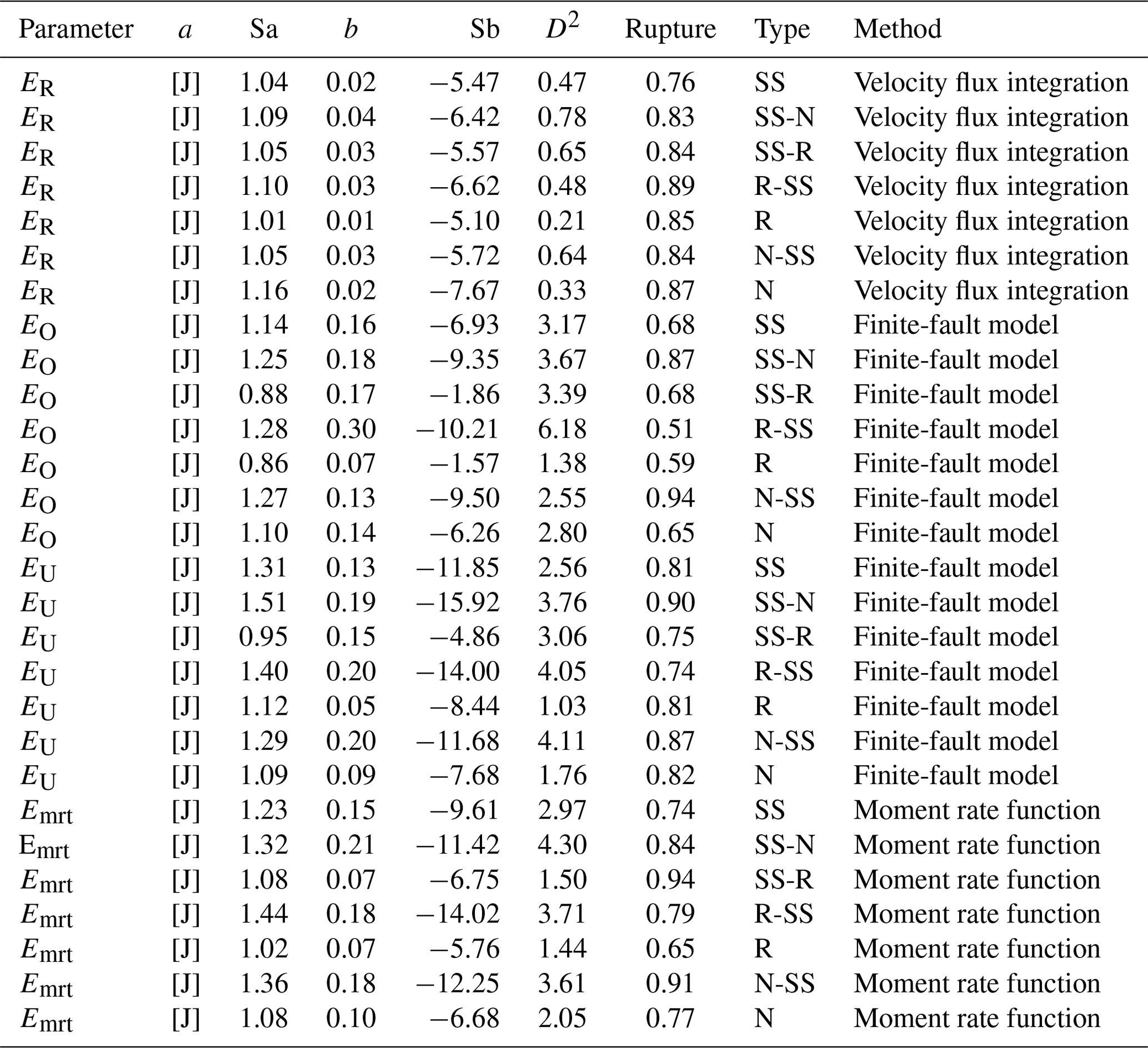
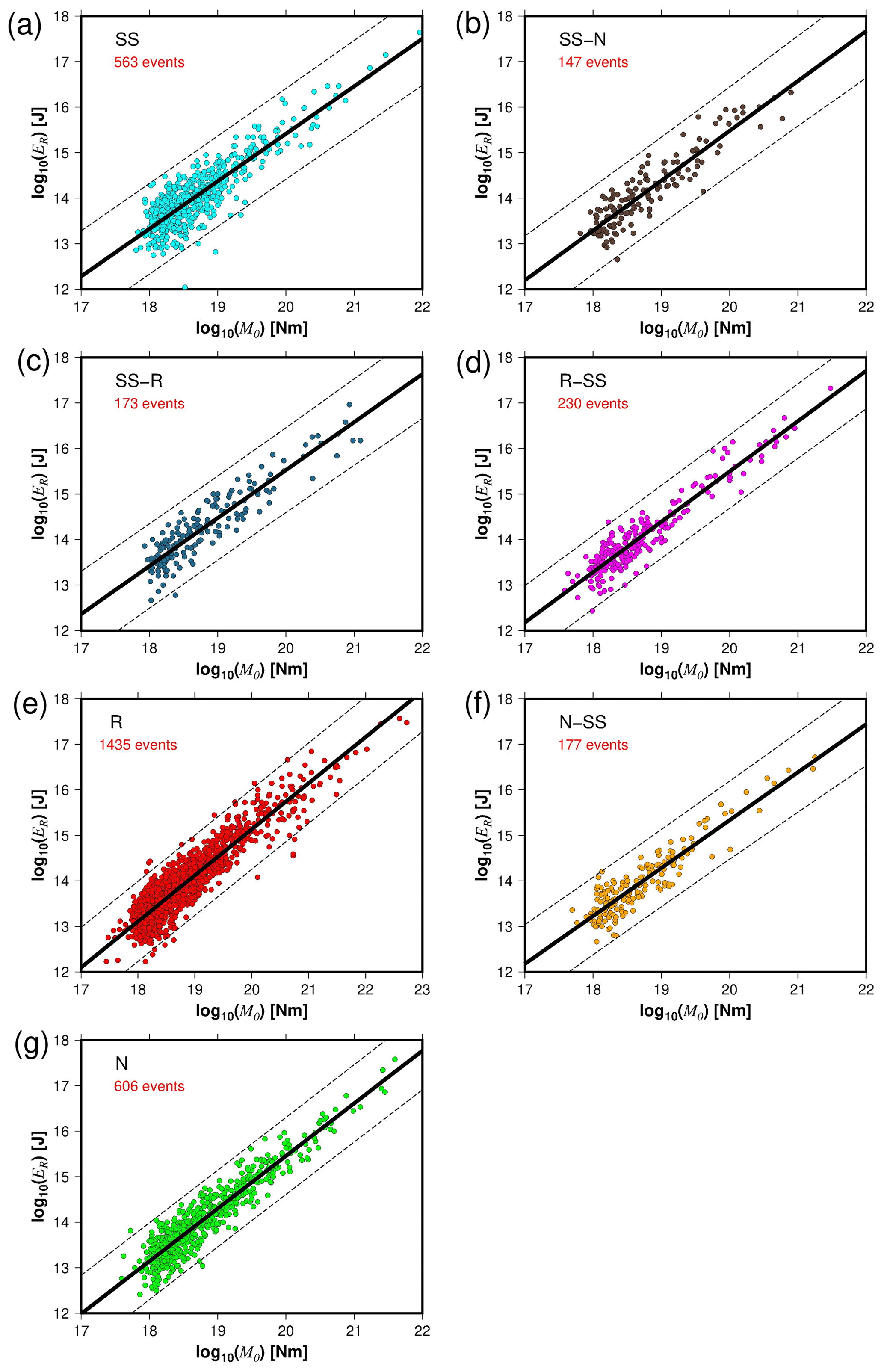
Figure 3 The radiated seismic energy (E_R) as a function of the seismic moment (M₀) for the different rupture types (a–g). The solid black lines represent the best fit, and the dashed lines indicate the 95 % confidence interval about the regression lines.

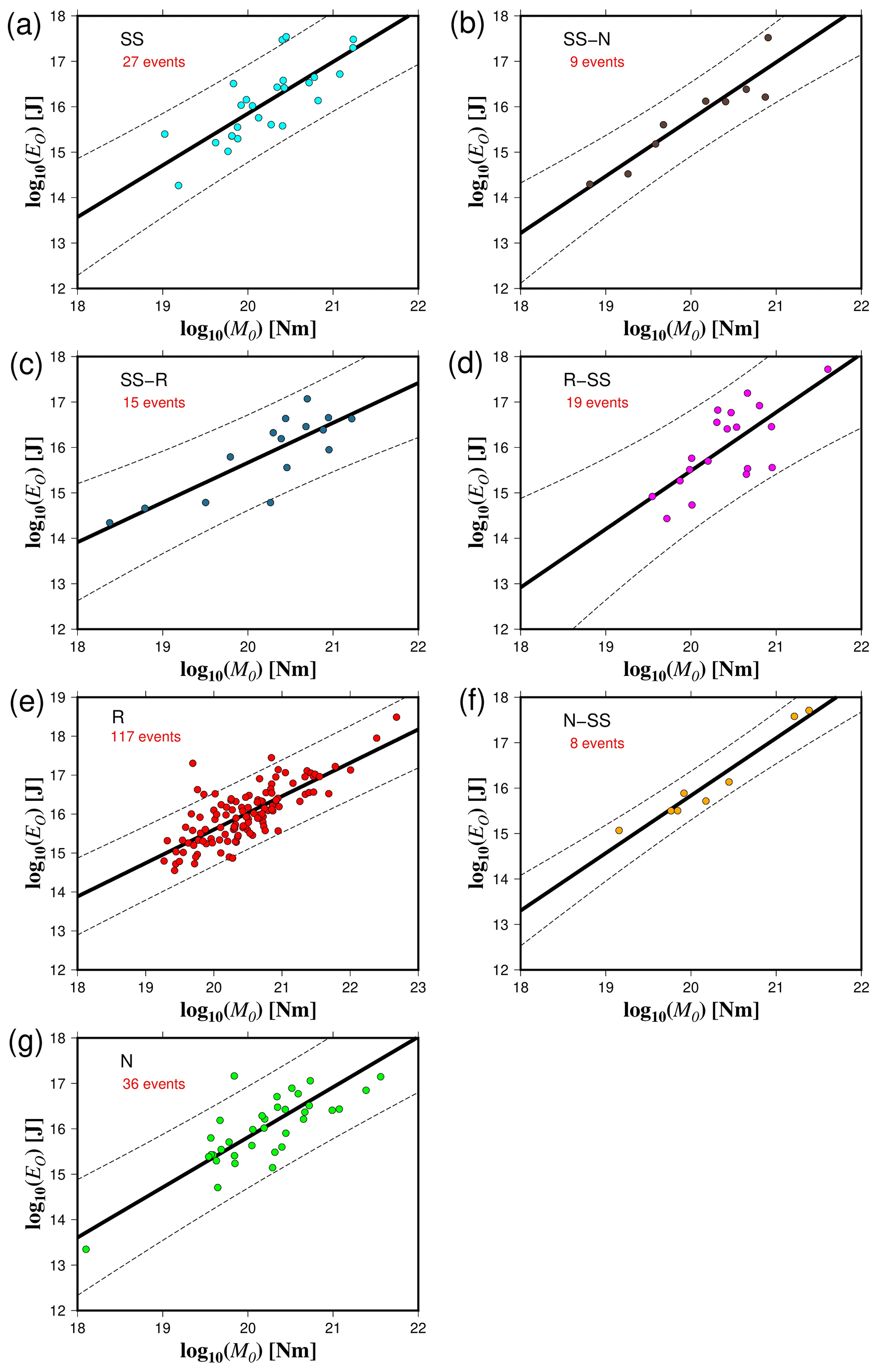
Figure 4 The overdamped dynamics approximation of the radiated energy (E_O) as a function of the seismic moment (M₀) for the different rupture types (a–g). The solid black lines represent the best fit, and the dashed lines indicate the 95 % confidence interval about the regression lines.

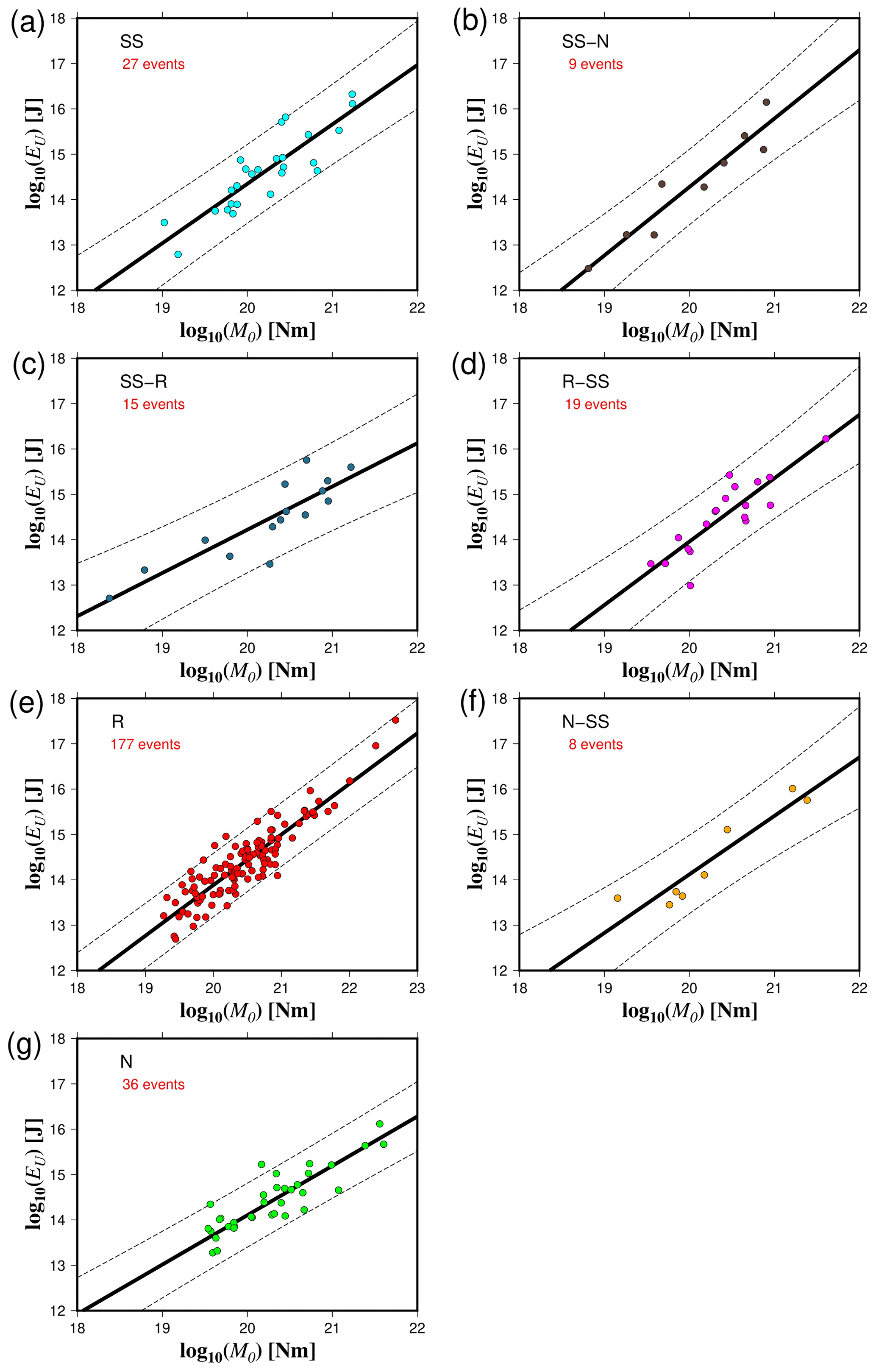
Figure 5 The energy obtained from the averaged finite-fault model (E_U) as a function of the seismic moment (M₀) for the different rupture types (a–g). The solid black lines represent the best fit, and the dashed lines indicate the 95 % confidence interval about the regression lines.

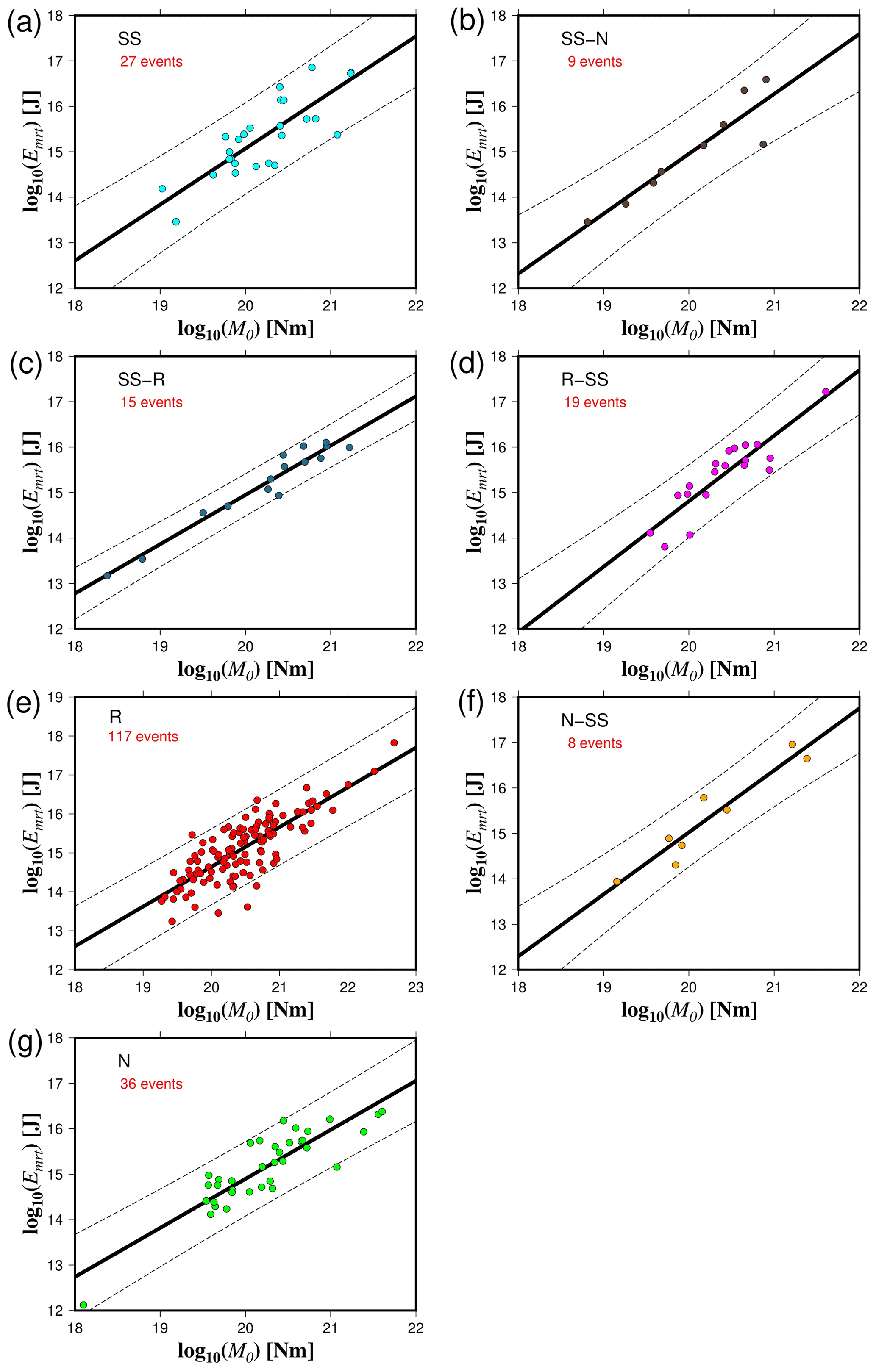
Figure 6 The radiated seismic energy based on moment rate functions (E_rmt) versus seismic moment (M₀) for the different rupture types (a–g). The solid black lines represent the best fit, and the dashed lines indicate the 95 % confidence interval about the regression lines.

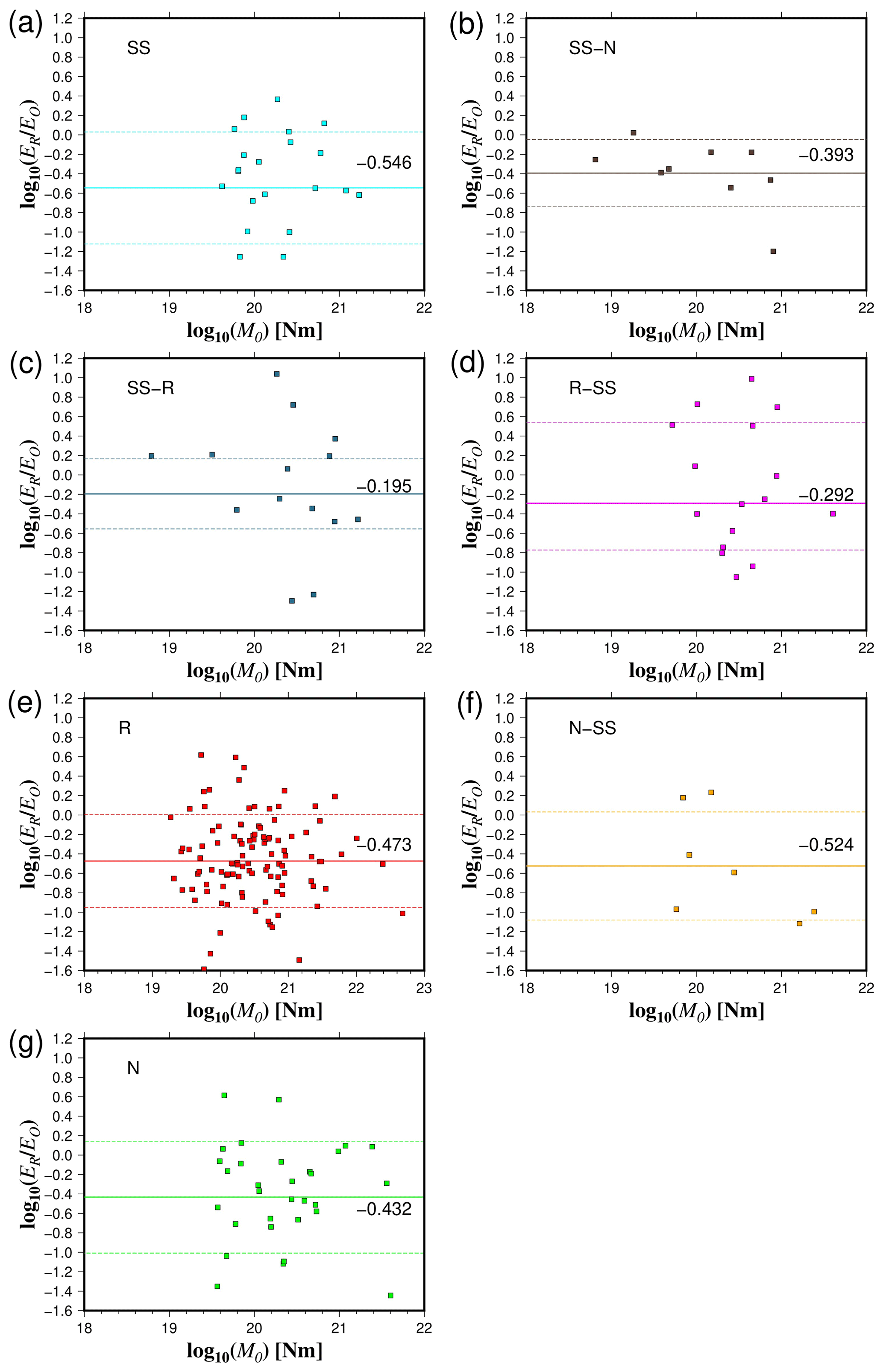
Figure 7 Comparison between radiated seismic energy based on velocity flux integration (E_R) and overdamped (E_O) energy estimations (a–g). Lines represent the mean values (continuous) of different rupture types and their standard deviations (dashed).

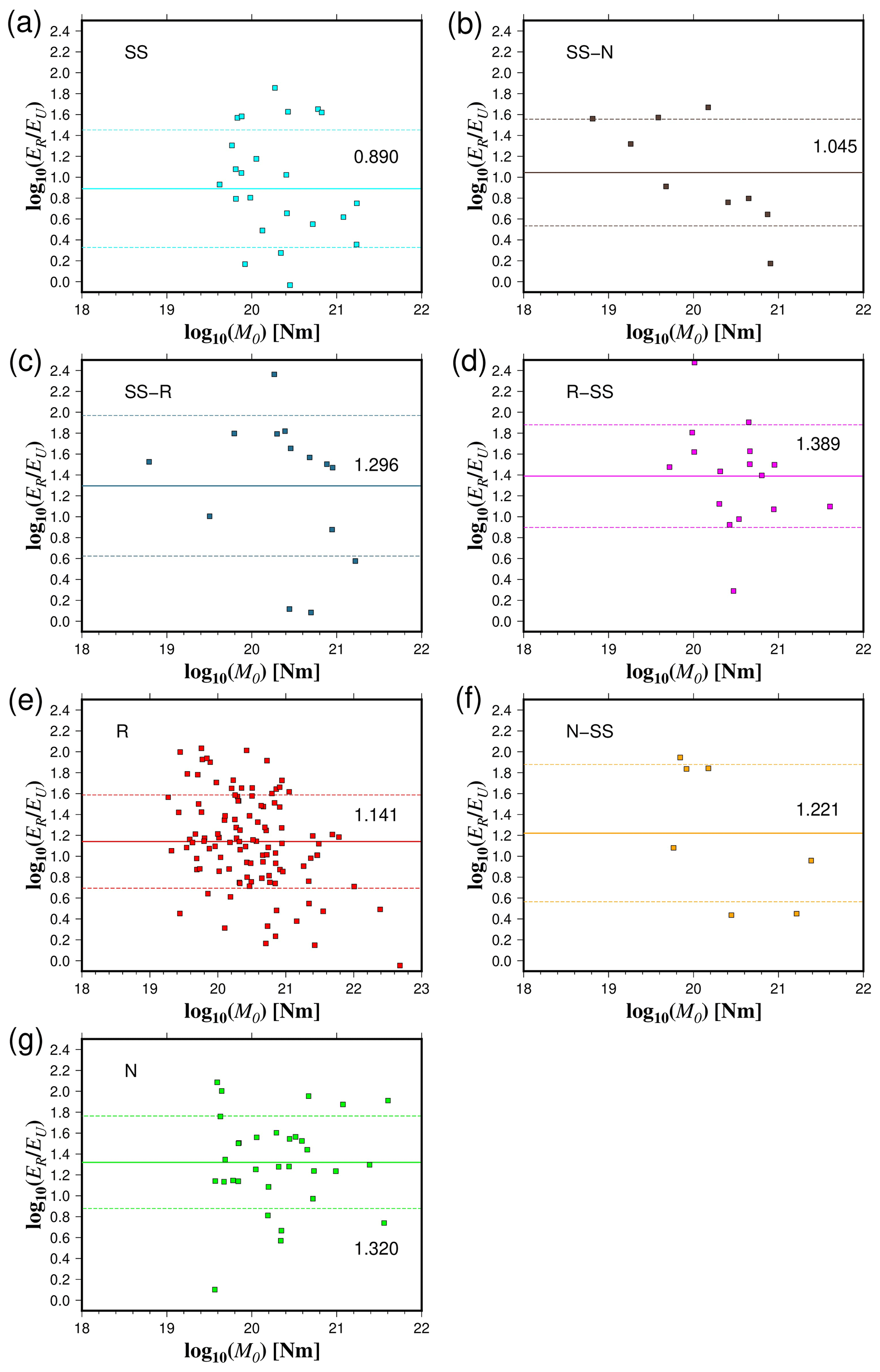
Figure 8 Comparison between the ratio of radiated seismic energy based on velocity flux integration (E_R) and averaged finite-fault model energy (E_U) estimations as a function of seismic moment (a–g). Lines represent the mean values (continuous) of different rupture types and their standard deviations (dashed).

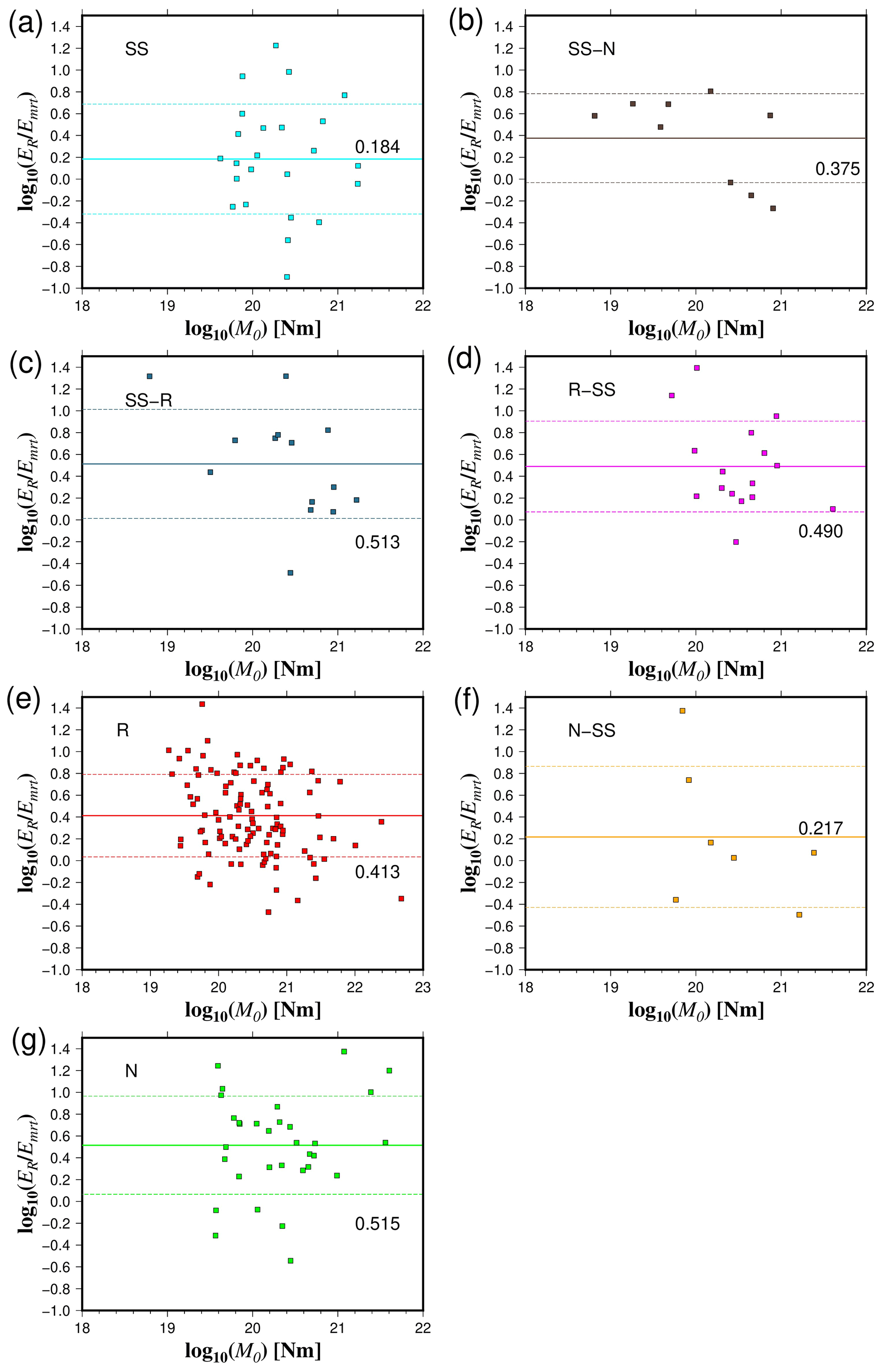
Figure 9 Comparison between the ratio of radiated seismic energy based on velocity flux integration (E_R) and moment rate (E_mrt) energy estimations as a function of seismic moment (a–g). Lines represent the mean values (continuous) of different rupture types and their standard deviations (dashed).

Table 2 Conversion relationships among the different types of energies. E_R is the radiated seismic energy based on velocity flux integration, E_O is the overdamped dynamics approximation of the radiated energy, E_U is the energy obtained from the averaged finite-fault model, and E_mrt is the energy obtained from moment rate functions.

3 Results

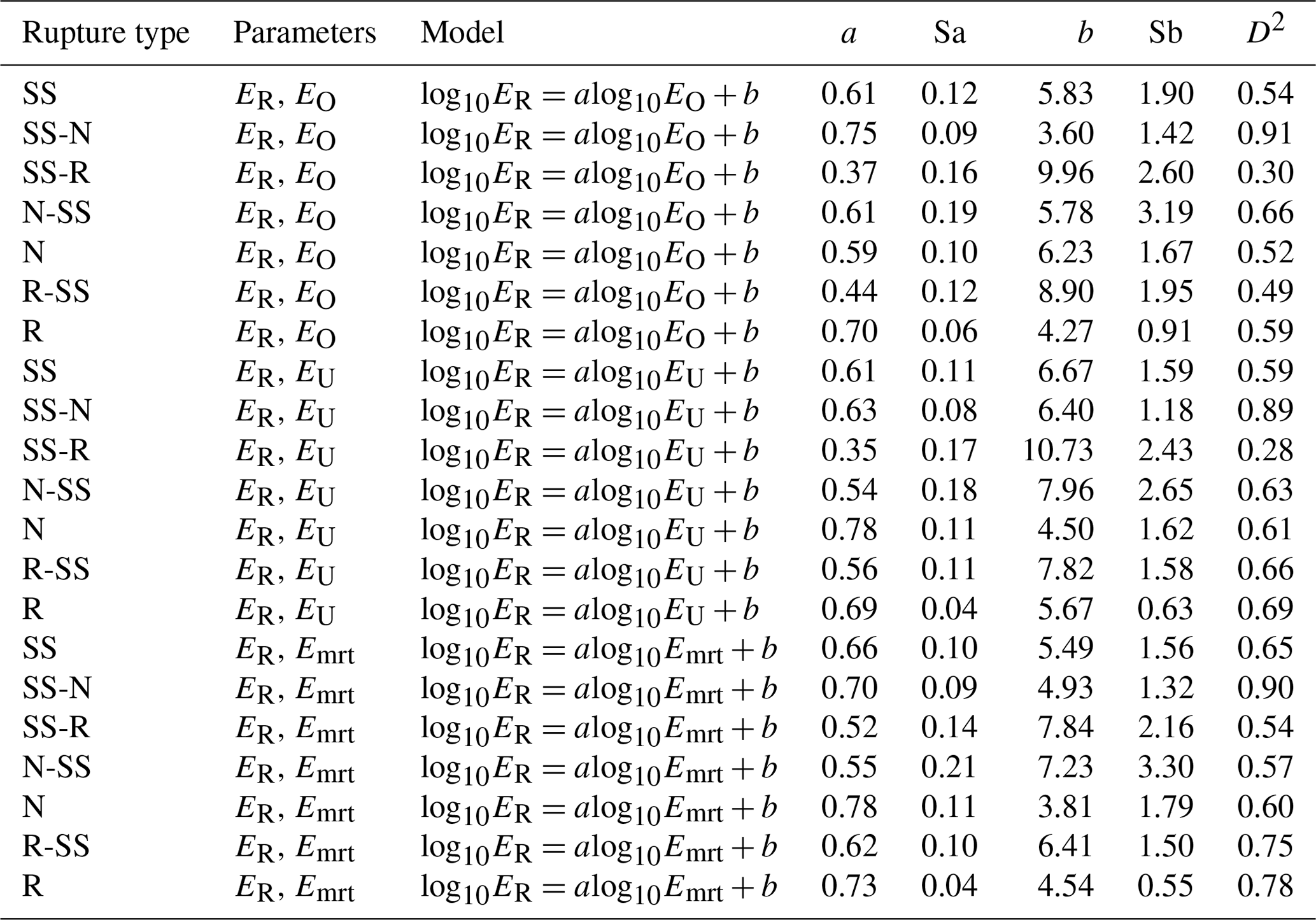
We used different methods to quantify the radiated seismic energy. Table 1 shows the calculated scaling relationships for E_R for each energy method and type of faulting. Figures 3–6 display the energy scaling relations derived from the velocity flux integration (E_R), overdamped dynamics approximation (E_O), the uniform model energy estimation (E_U), and moment rate function methods (E_mrt), respectively. Our results show some disparities in the calculated radiated seismic energies obtained with different techniques and data types. After carrying out rigorous statistical t tests, when comparing E_R with the other methods to estimate seismic energy, we find that E_O estimates are always lower than E_mrt and E_U, while E_U's estimates are the highest (Tables S1 to S3 in the Supplement). The lowest average difference factors are for E_O estimates, ranging from 0.28 to 0.77 (Fig. 7). Conversely, mean difference factors can be as high as 20 for E_U estimations (Fig. 8). Average difference factors exhibit intermediate values for E_mrt calculations, fluctuating from 1.53 to 3.27 (Fig. 9). These relations stand regardless of the rupture type (Tables S1 to S3, and Figs. 7 to 9). Conversion relationships between E_R and E_O, E_U, and E_mrt are presented in Table 2, which may be helpful when considering either estimation method.

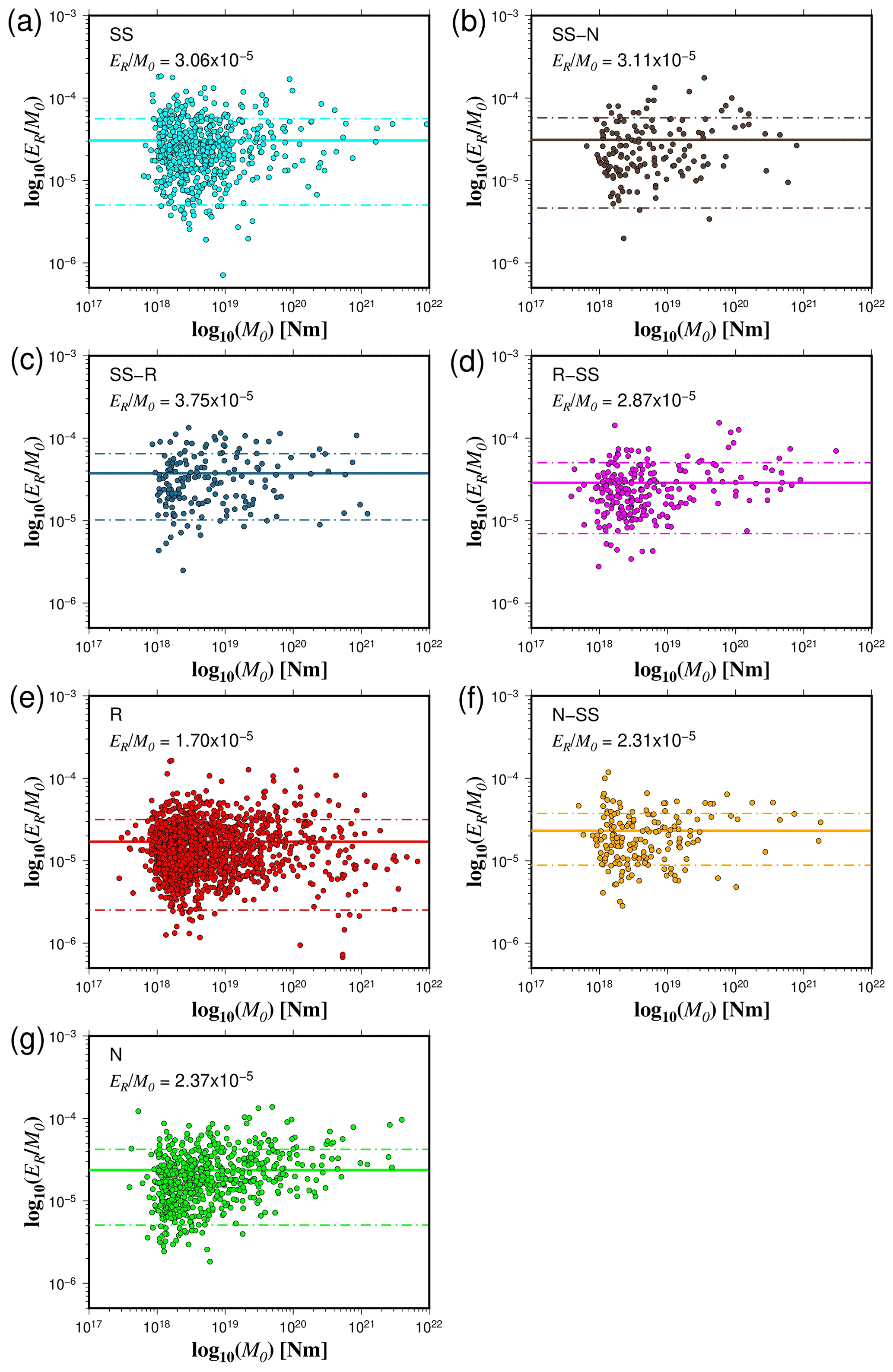
Figure 10 The estimated energy-to-moment ratios plotted as a function of the seismic moment for all the rupture types (a–g). The solid and dashed lines show the mean values and standard deviations, respectively.

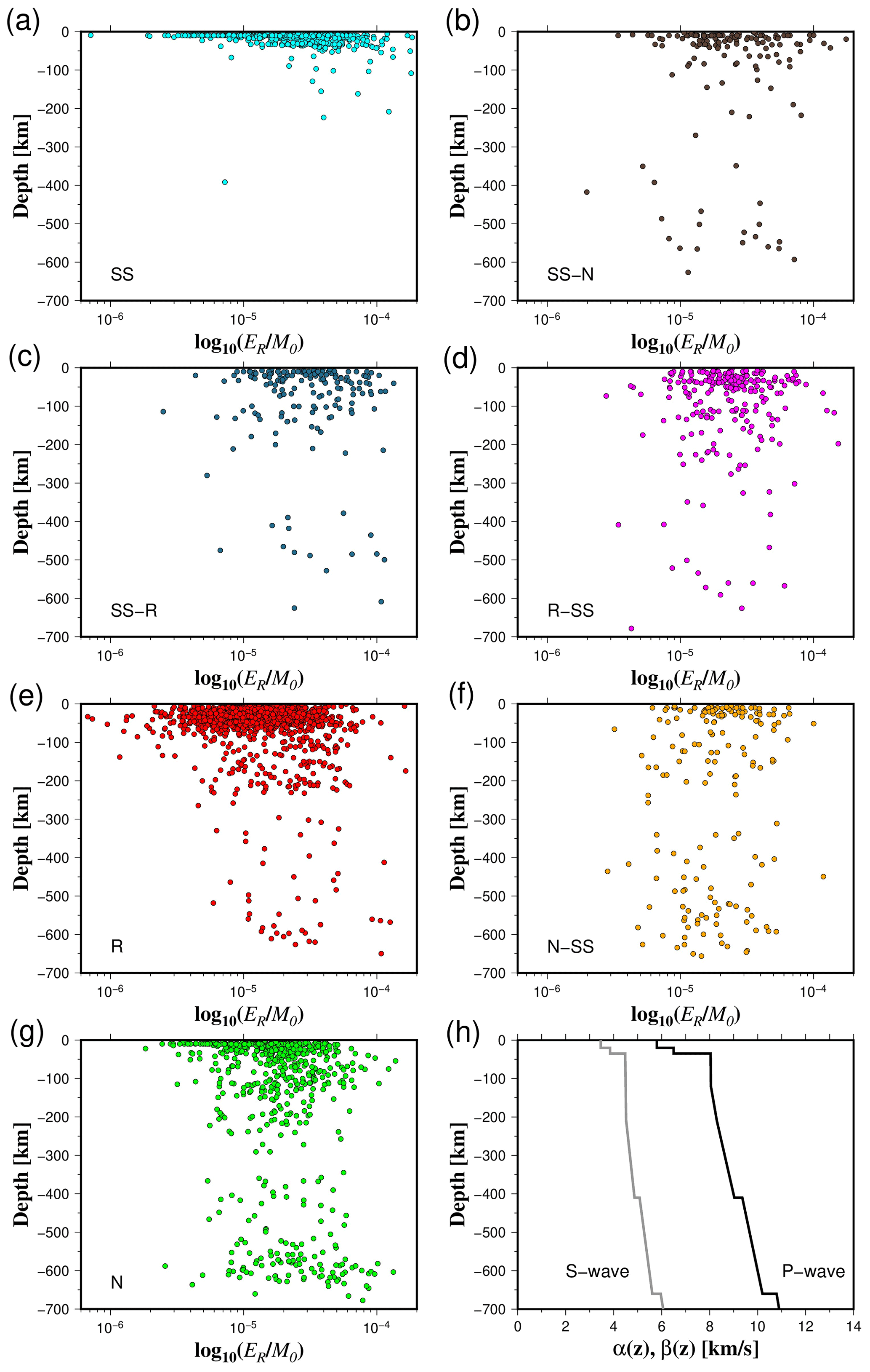
Figure 11 Energy-to-moment ratios with respect to depth for all rupture types (a–g). Panel (h) shows the ak135-F global velocity model.

In terms of the $E_{\mathrm{R}}/M_{\mathrm{0}}$ ratio, our results show that SS, SS-N, and SS-R events have the highest mean values (3.06 × 10⁻⁵ < $E_{\mathrm{R}}/M_{\mathrm{0}}$ < 3.75 × 10⁻⁵) (Fig. 10). R-SS earthquakes have a slightly lower mean ratio ($E_{\mathrm{R}}/M_{\mathrm{0}}$ = 2.87 × 10⁻⁵) (Fig. 10). Average $E_{\mathrm{R}}/M_{\mathrm{0}}$ ratio fluctuates from 2.31 × 10⁻⁵ to 2.37 × 10⁻⁵ for N-SS and N events, respectively (Fig. 10). On the other hand, the lowest values of $E_{\mathrm{R}}/M_{\mathrm{0}}$ are related to R earthquakes ($E_{\mathrm{R}}/M_{\mathrm{0}}$ = 1.70 × 10⁻⁵) (Fig. 10). Statistical tests confirm this trend since we find that, in general, and for data where there is a significant difference, (SS, N-SS, R-SS, SS-N, SS-R) > N > R (Tables S4 to S10 in the Supplement). The same trend is repeated for events in the Z < 30 km, 30 < Z < 60 km, and 60 < Z < 90 km depth ranges. For the 90 < Z < 120 km depth range, we can only confidently state that R-SS > N and SS-R > N due to a lack of data. Most of the rupture types present differentiated $E_{\mathrm{R}}/M_{\mathrm{0}}$ behavior in terms of depth with the existence of two clusters, above and below about 300 km depth (Fig. 11). In contrast, strike-slip earthquakes demonstrate a distinct pattern, with the majority of $E_{\mathrm{R}}/M_{\mathrm{0}}$ observations concentrated at depths shallower than 50 km (Fig. 11). Furthermore, at shallow depths, the radiated energy-to-moment ratio shows large variability compared to observations of deep earthquakes (Fig. 11).

Table 3 Estimations of average apparent stress (τ_α) for different faulting types based on the velocity flux integration method. τ_α is calculated with the following model: log₁₀E_R = log₁₀M₀+b, where τ_α=μ10^b. We assume $\mathit{\mu }=\stackrel{\mathrm{‾}}{\mathit{\mu }}$ as the average rigidity in a specific depth interval of 30 km. ${\mathit{\tau }}_{\mathit{\alpha }}^{\mathrm{1}}$ and ${\mathit{\tau }}_{\mathit{\alpha }}^{\mathrm{2}}$ are the 95 % the upper and lower confidence intervals for the mean. ^a and ^b indicate τ_α results from Choy and Boatwright (1995) and Pérez-Campos and Beroza (2001), respectively (bottom lines).

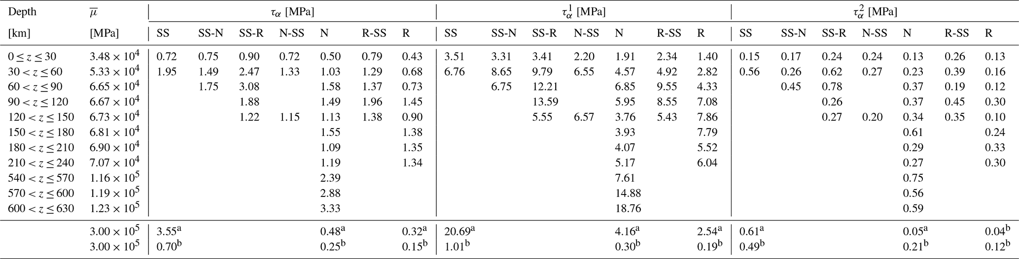
Previous studies have provided evidence that mean apparent stress estimates can be obtained using regression models, specifically through the equation log₁₀E_R = log₁₀M₀+b with τ_α = μ10^b, supporting the focal mechanism dependence of E_R (Choy and Boatwright, 1995; Pérez-Campos and Beroza, 2001). To test if this dependence persists with depth, we conducted regressions every 30 km of depth considering variations in μ and at least 10 observations. First, we evaluated reported seismic energy observations based on the velocity flux integration method (Table 3). Considering the distinct statistical differences in the $E_{\mathrm{R}}/M_{\mathrm{0}}$ ratios across various rupture types, we can justify that the τ_α results exhibit a similar pattern as they are derived through multiplication with a consistent scaling factor determined by the value of μ. Thus, our results agree with previous studies where τ_α follows the following behavior: (R-SS, R) < (N-SS, N) < (SS, SS-N, SS-R) in the range of 0–180 km (Table 3). Conversely, τ_α is higher for R events than for N earthquakes at depths from 180 to 240 km (Table 3). At depths greater than 240 km, only N events were obtained under the assumptions considered. In Table 3, we summarized results for all the depth intervals showing the mean values and their 95 % log-normal geometric spreads.

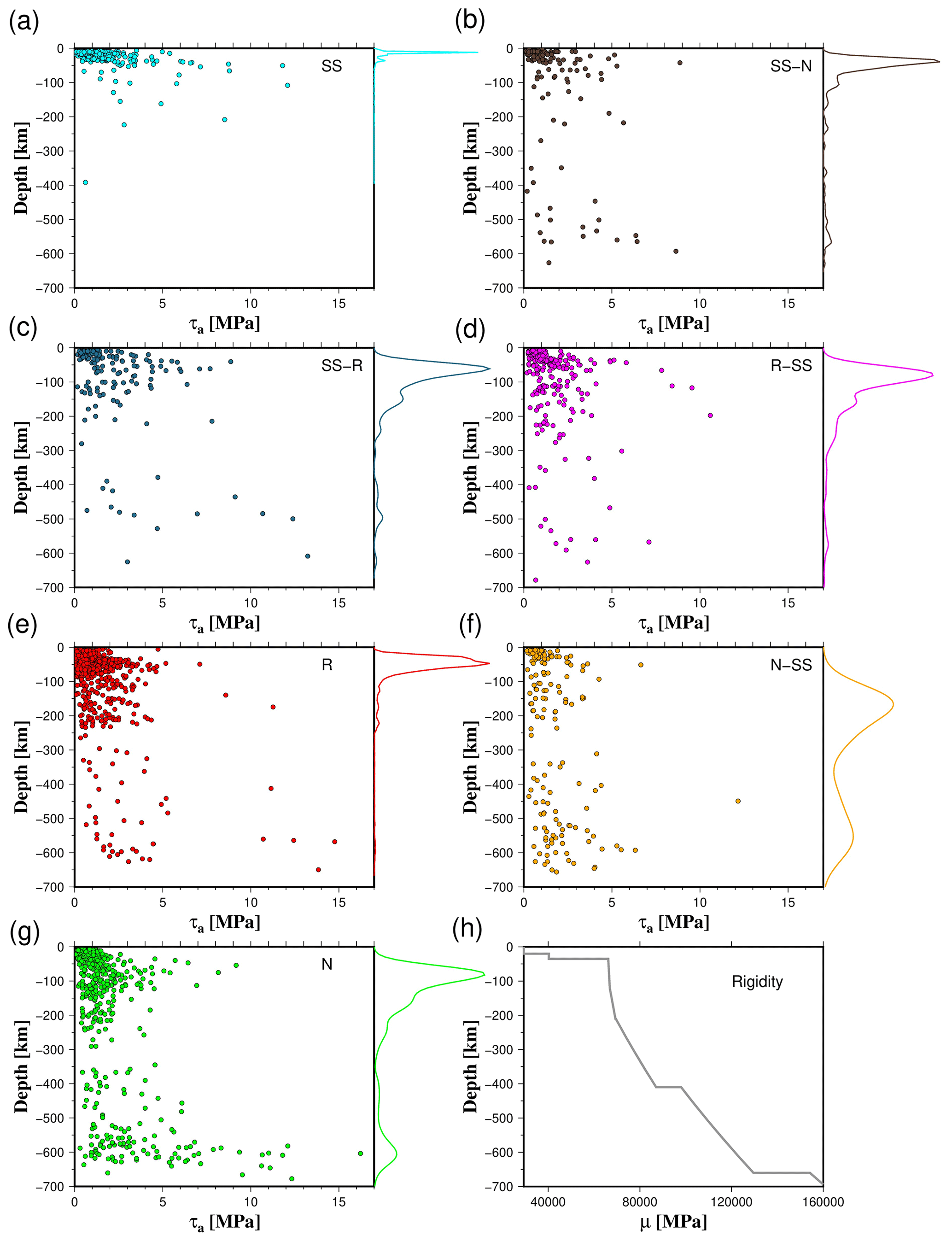
Figure 12 Apparent stress (τ_a) with respect to depth for all rupture types (a–g). Color curves are the probability density functions (PDFs). Rigidity vs. depth based on the ak135-F global velocity model employed in the estimation of τ_a (h).

Table 4 Estimations of average apparent stress (τ_α) for different faulting types based on slip distributions (E_mrt, E_U, and E_O). τ_α is calculated with the following model: log₁₀E_R = log₁₀M₀+b, where τ_α=μ10^b. We assume $\mathit{\mu }=\stackrel{\mathrm{‾}}{\mathit{\mu }}$ as the average rigidity in a specific depth interval of 30 km. ${\mathit{\tau }}_{\mathit{\alpha }}^{\mathrm{1}}$ and ${\mathit{\tau }}_{\mathit{\alpha }}^{\mathrm{2}}$ are the 95 % the upper and lower confidence intervals for the mean. ^a and ^b indicate τ_α results from Choy and Boatwright (1995) and Pérez-Campos and Beroza (2001), respectively (bottom lines).

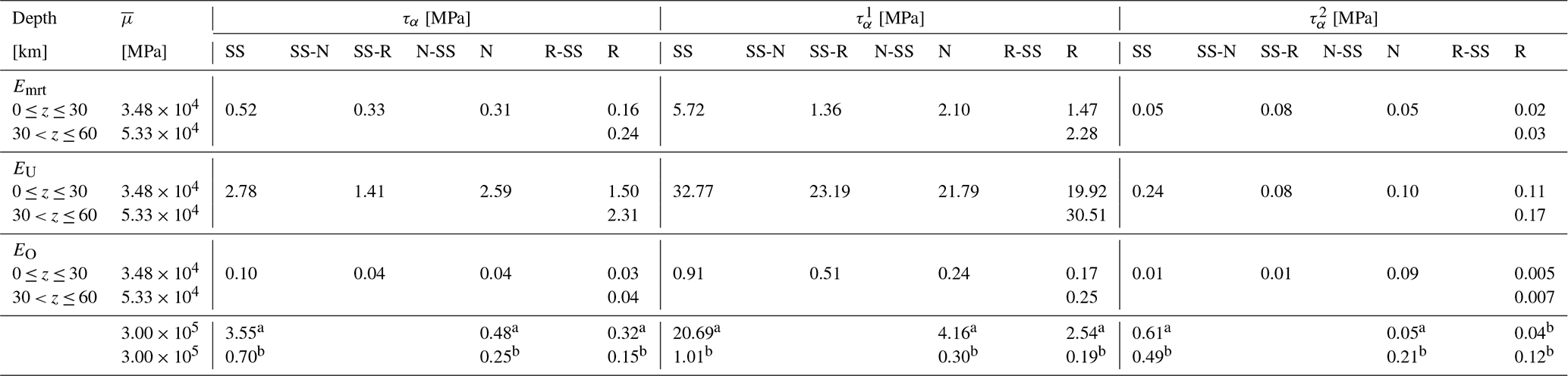
Our results also showed that N and N-SS events exhibit a bimodal distribution of τ_α with depth (Fig. 12). The most significant values of τ_α occur in two depth ranges of approximately 40–60 and 580–650 km, where maximum apparent stresses approach 8 and 16 MPa, respectively (Fig. 12). N-SS, R, R-SS, SS-N, and SS-R events also showed two maximum values of τ_α ranging from 7 to 11 MPa and 9 to 15 MPa for shallow and deep earthquakes, respectively (Fig. 12). For SS events, there is only one depth range over which τ_α shows maxima. In this case, the highest values of τ_α are found in the greater depth range from 50 to 100 km (τ_α ∼ 12 MPa) (Fig. 12). On the other hand, the average apparent stress estimates based on the finite-fault models exhibit a similar dependence on the focal mechanism than those obtained with the velocity flux integration method at shallow depths (Z < 30 km) (Table 4). Regressions showed that τ_α follows the following behavior: R < N < (SS, SS-R) for E_U and E_mrt estimations (Table 4). In contrast, E_O showed no clear dependence of τ_α with the focal mechanism (Table 4). Due to the constraint of at least 10 observations (slip distributions) for each 30 km depth interval, we could not analyze the dependence of τ_α on the type of faulting at a deeper depth.

4 Discussion

In this study, we analyzed radiated seismic energy and parameters that measure the amount of energy per unit of the moment, such as the apparent stress and the energy-to-moment ratio (also known as scaled energy or apparent strain), considering their respective particularities. The advantage of using τ_α is that it can be related to other stress processes associated with the seismic rupture, such as the stress drop. On the other hand, many finite-fault models of the spatiotemporal slip history for moderate and large earthquakes exist. From these models, important information can be extracted, such as fault dimensions (Mai and Beroza, 2000), static stress drop (Ripperger and Mai, 2004), or radiated seismic energy (Ide, 2002; Senatorski, 2014). When using finite-fault models to determine E_R, it is necessary to consider that they usually explain low-frequency seismic waves. However, the higher-frequency wave contribution is necessary for calculating the total radiated seismic energy. This issue brings differences among finite-fault energy estimates and those from integrating far-field waveforms.

Furthermore, finite-fault seismic energy estimations are strongly affected by event location, the number of available data, faulting parameterization, and velocity structure. The degree of discrepancy between the finite-fault energy estimates (E_mrt, E_O, and E_U) with respect to the velocity flux integration method (E_R) is variable among the different types of seismic energy. For example, the moment rate functions are relatively robustly determined by teleseismic data, while rupture dimensions are strongly affected by model parameters (Ye et al., 2016). This may explain why the average difference factor ($E_{\mathrm{R}}/E_{\mathrm{U}}$) is greater than the $E_{\mathrm{R}}/E_{\text{mrt}}$ factor (Figs. 8 and 9). Another source of discrepancies in finite-fault energy calculations comes from the spatial and temporal smoothing in resolving the kinematic slip distribution and the rupture velocity assigned. Errors associated with the assumptions are tough to quantify as they propagate into the energy estimates in complex ways.

Our results agree with previous estimates of E_O and E_U, confirming that E_R is in the range of E_U–E_O for most earthquakes. The overdamped approximation (E_O) can be used to characterize the heterogeneity of the rupture process. Senatorski (2014) states that if the ratio $E_{\mathrm{O}}/E_{\mathrm{R}}$ is < 0.4, the rupture can be represented as a simple dislocation rupture. $E_{\mathrm{O}}/E_{\mathrm{R}}$ > 1 is expected in the case of heterogeneous rupture processes. On the other hand, some of the suggested explanations for the observation that E_O > E_R are (1) the finite-fault slip models require refinement; (2) the seismic energy estimations require correction for directivity, modified attenuation factors, or sites effects; and (3) some other factors that are not considered in the calculations, such as the fact that the energy dissipation is not taken into account by the planar faults (Senatorski, 2014).

The radiated seismic energy scaled by seismic moment is an essential characterization of earthquake dynamics. The low $E_{\mathrm{R}}/M_{\mathrm{0}}$ of reverse events is associated with tsunami earthquakes being compatible with the results of previous studies (Newman and Okal, 1998; Venkataraman and Kanamori, 2004a; Convers and Newman, 2011; Ye et al., 2016). Our results showed that $E_{\mathrm{R}}/M_{\mathrm{0}}$ has a large scatter from 6 × 10⁻⁷ to 2 × 10⁻⁴ for all the rupture types. However, no evident magnitude dependence can be asserted (Fig. 10). One of the reasons for the dispersion of $E_{\mathrm{R}}/M_{\mathrm{0}}$ is that it depends on many seismogenic properties of the source region (Fig. 10). As a consequence, $E_{\mathrm{R}}/M_{\mathrm{0}}$ varies significantly in different tectonic environments and deep conditions such as pressure and temperature (Fig. 11). Even within the same tectonic environment, $E_{\mathrm{R}}/M_{\mathrm{0}}$ has significant variations, as has been reported by Plata-Martínez et al. (2019) in the Middle American Trench, where variations in $E_{\mathrm{R}}/M_{\mathrm{0}}$ are associated with heterogeneities along the trench, such as asperities. The different types of earthquakes have differences in the frequency content of the seismic energy released.

Venkataraman and Kanamori (2004a) reported that $E_{\mathrm{R}}/M_{\mathrm{0}}$ is in the range of 5 × 10⁻⁶ to 2 × 10⁻⁵ for interplate and downdip earthquakes, which are mainly consistent with reverse and normal faulting. Our results show that the average values of $E_{\mathrm{R}}/M_{\mathrm{0}}$ for R and N events are 1.70 × 10⁻⁵ and 2.37 × 10⁻⁵, respectively, and both values are within the interval defined by Venkataraman and Kanamori (2004a). The $E_{\mathrm{R}}/M_{\mathrm{0}}$ ratio for deep earthquakes varies from 2.0 × 10⁻⁵ to 3.0 × 10⁻⁴ (Venkataraman and Kanamori, 2004a). We found that $E_{\mathrm{R}}/M_{\mathrm{0}}$ for deep earthquakes of all types of rupture is in the interval of 2 × 10⁻⁶ to 2 × 10⁻⁴ but with a predominance of 1.0 × 10⁻⁵ > $E_{\mathrm{R}}/M_{\mathrm{0}}$ (Fig. 11). Despite the $E_{\mathrm{R}}/M_{\mathrm{0}}$ scatter, our results depict a general trend for the average values of $E_{\mathrm{R}}/M_{\mathrm{0}}$, which can be expressed as R < (N, N-SS, R-SS) < (SS, SS-R, SS-N) (Fig. 10); a similar tendency was reported by Convers and Newman (2011), where $E_{\mathrm{R}}/M_{\mathrm{0}}$ follows R < N < SS.

Our results support E_R's previously reported focal mechanism dependence (Choy and Boatwright, 1995; Pérez-Campos and Beroza, 2001; Convers and Newman, 2011) but narrow the range. Examination of mean τ_α with various focal mechanisms and at different depths has been done for different earthquake sizes and tectonic settings. We identified the largest values of apparent stress for strike-slip events, intermediate values for normal-faulting events, and lowest for reverse-faulting events in the depth interval of 0–180 km (Table 3). On the other hand, our results showed that at depths between 180 and 240 km, τ_α for reverse earthquakes is higher than for normal-faulting events. This can be explained; for example, deep reverse earthquakes in subduction zones occur in the slab's lower part, where they are subjected to significantly large compressive stresses. A precise characterization of the depth dependence of τ_α remains unclear at depths greater than 240 km. In Table 3, we present and compare our results for τ_α, supporting the observation of the dependence of E_R on the type of faulting. The origin of this focal dependence is unclear, but it has been raised that it reflects a mechanism-dependent difference in stress drop (Pérez-Campos and Beroza, 2001). This can be highlighted with an alternative definition for the apparent stress, assuming that the dynamic and static stress drops are roughly equivalent. Then τ_α can be expressed as τ_α = (${\mathit{\eta }}_{\mathrm{R}}\mathrm{\Delta }\mathit{\sigma })/\mathrm{2}$, where η_R is the seismic efficiency and Δσ is the stress drop (Convers and Newman, 2011). Allmann and Shearer (2009) provided additional information to support the role of stress drop in the dependency of apparent stress with the type of faulting. They found a dependence of median stress drop on the focal mechanism with a factor of 3–5 times higher stress drops for strike-slip events and 2 times higher stress drops for intraplate events compared to interplate events.

Nevertheless, other interpretations of the apparent stress variation are related to the mechanical properties of the rock, such as the reduction in rigidity in shallow subduction environments or increment in lithostatic pressure if no change in regional rigidity is assumed (Convers and Newman, 2011). The variation in such estimates concerning expected spatial variations in rigidity is an issue that still needs attention. Choy and Kirby (2004) also suggested that τ_α can be related to fault maturity. For example, lower stress drops are needed to reach rupture in mature faults. Conversely, earthquakes generated at immature faults (low cumulative displacement) radiate more energy per unit of seismic moment. Regarding the behavior of τ_α with depth, our results agree with the existence of a bimodal distribution with two depth intervals where the apparent stress is maximum for normal-faulting earthquakes, as reported by Choy and Kirby (2004). We also found that almost all types of faulting (SS-N, SS-R, R-SS, R, N-SS, and N) show two depth ranges where the stress is maximum, but in the case of normal-faulting earthquakes, it is very well defined. On the other hand, almost all strike-slip earthquakes show a single interval of depths where the apparent stress is maximum (Fig. 12). Earthquakes with an oblique focal mechanism show a mixed behavior of τ_α, as is the case of the SS-N and SS-R events that present similar characteristics to normal and reverse earthquakes in terms of the depth distribution of τ_α.

In terms of the spatial distribution ofE_R and τ_α (Figs. S1 to S14 in the Supplement), the highest values of τ_α for N events are located at the border between the Nazca and South American plates, the Eurasian and Philippine plates, the Indo-Australian and Pacific plates, the Philippine and Pacific plates, and the Pacific and North American plates (in the Alaska region) (Fig. S1). Regarding the seismic energy of earthquakes, the regions where the most energetic earthquakes have occurred concur with the aforementioned areas, with the addition of the border between the Cocos and North American plates (Fig. S2). The high τ_α normal-faulting events are associated with regions of intense deformation, such as a sharp slab bending or zones where opposing slabs collide (Choy and Kirby, 2004). At shallow depths (Z < 35 km), high-τ_α events are related to the beginning of the subduction beneath the overriding plate (Choy and Kirby, 2004). Our results support the observation that the average apparent stress of intraslab normal-faulting events is considerably higher than the average τ_α of interplate thrust-faulting earthquakes reported by Choy and Kirby (2004) (Figs. S1 and S5).

In the case of R earthquakes, the highest values of E_R and τ_α are in the limit of the Eurasian and Philippine plates, the Nazca and South American plates, the Philippine and Pacific plates, the Indo-Australian and Pacific plates, and the Eurasian and Indo-Australian plates (Figs. S5 and S6). In contrast, strike-slip events with the highest values of E_R and τ_α are on the border between the African and Eurasian plates (in Türkiye), the Eurasian and Indo-Australian plates, the Philippine and Eurasian plates, the Indo-Australian and Pacific plates (in New Zealand), and the Caribbean and South American plates (Figs. S13 and S14). We have found that several SS earthquakes are located in the oceanic lithosphere at depths < 50 km. Many of the SS events with high τ_α are located near plate-boundary triple junctions where there are high rates of intraplate deformation, as previously reported by Choy and McGarr (2002).

Finally, when using seismic energy estimates based on finite-fault models (E_O and E_mrt), a clear dependence of the average apparent stress with the focal mechanism is observed at shallow depths (Z < 30 km) (Table 4). For example, using E_U and E_mrt, the average τ_α follows R < N < (SS-R, SS). If E_O is used, the mean apparent stress exhibits similar values for SS-R, N, and R events (Table 4). However, the lack of a significant number of observations for some types of earthquakes makes it challenging to evaluate the use of finite-fault models to determine apparent stress. Despite these limitations, the methods used to estimate the seismic energy based on finite-fault models are a quick alternative to calculate a range of energy variation once a slip distribution is obtained. Determining earthquake occurrence rates from the accumulated seismic moment is an established tool of seismic hazard analysis. The size of an earthquake can also be defined in terms of the radiated seismic energy. Incorporating the spatial distribution of seismic energy in seismic hazard analyses has the advantage that seismic energy is a better predictor of the damage potential of seismic waves than the seismic moment release. In that sense, our results can be used to improve global seismic hazard models.

5 Conclusion

We studied the radiated seismic energy, energy-to-moment ratio, and apparent stress of different types of faulting. Our data rely on different methodologies employing the velocity flux integration and finite-fault models to determine the seismic energy. The approach based on slip distributions involved the utilization of two techniques: (1) total moment rate functions and (2) overdamped dynamics approximation. We analyzed 3331 energy observations derived from integrating far-field waveforms. On the other hand, we used 231 finite-fault models. For all mechanism types, E_U > E_mrt > E_O, based on statistical t tests. Finite-fault energy estimations also support focal mechanism dependence of apparent stress but only for shallow earthquakes (Z < 30 km). The population of slip distributions used was too small to conclude that finite-fault energy estimations support the dependence of average apparent stress on rupture type at different depth intervals. The estimated energy differences are within the margin reported in the literature, which can reach a factor greater than 10. The methods used to estimate seismic energy based on finite-fault models are an easily implemented alternative that give results compatible with the seismic record integration technique, given the larger uncertainties of these methods. We also derived scaling relationships for the different types of energies and conversion relations.

In terms of the behavior of the $E_{\mathrm{R}}/M_{\mathrm{0}}$ ratio, our results showed a high scatter without a clear dependence on magnitude. The $E_{\mathrm{R}}/M_{\mathrm{0}}$ ratio is, based on statistical t tests, the largest for strike-slip earthquakes, followed by normal-faulting events, with the lowest values for reverse earthquakes for hypocentral depths < 90 km. Not enough data are available for statistical tests at deeper intervals except for the range 90 to 120 km, where we can satisfactorily conclude that $E_{\mathrm{R}}/M_{\mathrm{0}}$ for R-SS and SS-R types is larger than for N-type faulting, which also conforms to the previous assumption. Regarding the behavior of τ_α with depth, our results agree with the existence of a bimodal distribution with two depth intervals where the apparent stress is maximum for normal-faulting earthquakes. At depths in the range of 180–240 km, τ_α for reverse earthquakes is higher than for normal-faulting events. Our $E_{\mathrm{R}}/M_{\mathrm{0}}$ estimates for deep earthquakes are also consistent with reported values. By analyzing the average apparent stress, our results also support the previously reported focal mechanism dependence of E_R at depths ranging from 0 to 180 km. We found that normal-faulting events have intermediate values of τ_α between strike-slip and reverse events using the energy flux integration approach in agreement with previous studies.

On the other hand, τ_α for reverse earthquakes is higher than for normal-faulting events at depths between 180 and 240 km. In contrast, a clear focal mechanism dependence is observed when finite-fault methods are used to estimate the mean apparent stress at shallow depths (Z < 30 km). This study's population of slip distributions was too small to conclude that finite-fault energy estimations support the mechanism dependence of average apparent stress at different depths. There are two depth ranges over which apparent stress for SS-N, SS-R, R-SS, R, N-SS, and N earthquakes shows maxima. Earthquakes with an oblique focal mechanism show a mixed behavior of energy parameters since it has common characteristics of two types of faults; in some cases, one of them predominates over the other.