Comparison of surface-wave techniques to estimate S- and P-wave velocity models from active seismic data

The acquisition of seismic exploration data in remote locations presents several logistical and economic criticalities. The irregular distribution of sources and/or receivers facilitates seismic acquisition operations in these areas. A convenient approach is to deploy nodal receivers on a regular grid and to use sources only in accessible locations, creating an irregular source–receiver layout. It is essential to evaluate, adapt, and verify processing workflows, specifically for near-surface velocity model estimation using surface-wave analysis, when working with these types of datasets. In this study, we applied three surface-wave techniques (i.e., wavelength–depth (W/D) method, laterally constrained inversion (LCI), and surface-wave tomography (SWT)) to a large-scale 3D dataset obtained from a hard-rock site using the irregular source–receiver acquisition method. The methods were fine-tuned for the data obtained from hard-rock sites, which typically exhibit a low signal-to-noise ratio. The wavelength–depth method is a data transformation method that is based on a relationship between skin depth and surface-wave wavelength and provides both S- and P-wave velocity (V_s and V_p) models. We used Poisson's ratios estimated through the wavelength–depth method to constrain the laterally constrained inversion and surface-wave tomography and to retrieve both V_s and V_p also from these methods. The pseudo-3D V_s and V_p models were obtained down to 140 m depth over an area of approximately 900 × 1500 m². The estimated models from the methods matched the geological information available for the site. A difference of less than 6 % was observed between the estimated V_s models from the three methods, whereas this value was 7.1 % for the retrieved V_p models. The methods were critically compared in terms of resolution and efficiency, which provides valuable insights into the potential of surface-wave analysis for estimating near-surface models at hard-rock sites.

1 Introduction

In order to overcome the difficulties of collecting seismic data in remote areas such as foothills and forests, a new acquisition method has been recently introduced, in which the nodal receivers are deployed in a regular grid, while the source locations are restricted to reachable areas such as the access roads (Lys et al., 2018). This approach creates an irregular source–receiver outline that raises the necessity to evaluate, verify, and test the seismic processing workflow. Here, we focus on the application of surface-wave methods to the data recorded through an irregular source–receiver scheme with the purpose of near-surface velocity model estimations. These velocity models can be used for engineering purposes or as input in the exploration processing workflow to improve static corrections and ground roll removal.

Surface-wave methods are powerful tools for subsurface characterization. Most of these methods process the data to extract the surface-wave phase velocity dispersion curve (DC) from seismic records and invert these DCs individually to estimate the velocity models. Since the energy decay of surface-wave wavefields in depth depends on their wavelength, the investigation depth of surface-wave methods is related to the maximum recovered wavelength and can be considerably variable, ranging from a few meters (e.g., Xia et al., 2002; Feng et al., 2005; Comina et al., 2011; Pan et al., 2018) to several tens of meters (e.g., Mordret et al., 2014; Da Col et al., 2020) or even to a few kilometers (e.g., Ritzwoller and Levshin, 1998; Kennett and Yoshizawa, 2002; Fang et al., 2015). The estimated models from surface-wave techniques can be used in many applications, such as near-surface site characterization (Lai, 1998; Xia, 2014; Foti et al., 2015), static corrections (Mari, 1984; Roy et al., 2010), and ground roll prediction and damping (Blonk and Herman, 1994; Ernst et al., 2002; Halliday et al., 2010).

Different methods can be adopted for extracting DCs from the seismic records and inverting them (see, for instance, Papadopoulou (2021) for a thorough review of the different processing techniques and characteristics of the estimated DCs). The retrieval of a velocity model from the DC can be based on simple data transformations or on model optimization approaches with different inversion strategies. According to the chosen workflow, the computational cost and model resolution may vary, and identifying the optimal approach for the analysis is an important task. Here, we compare three different methods (i.e., wavelength–depth data transform, laterally constrained inversion, and surface-wave tomography) that are rarely used for near-surface 3D model estimation. We apply these methods to a large-scale test dataset acquired from irregular deployed source–receiver layout. The data were collected from a hard-rock site, which is typically characterized by a lower signal-to-noise ratio compared to data from loose granular material (Papadopoulou, 2021).

Regardless of the type of surface-wave technique, since phase velocity DCs are known to have lower sensitivity to P-wave velocity (V_p) compared to S-wave velocity (V_s), most surface-wave methods focus on V_s estimation, and they require a priori Poisson's ratio or V_p for the inversion stage. Recently, a data transformation method based on the so-called wavelength–depth (W/D) relationship was developed to estimate both V_s and V_p models (Khosro Anjom et al., 2019). The W/D relationship is obtained by computing wavelength–depth couples corresponding to equal phase velocity of surface waves and time-average V_s and represents the skin depth of surface waves (Socco et al., 2017). Once estimated, the W/D relationship can be used to directly estimate the time-average V_s from DCs. Socco and Comina (2017) showed with synthetic tests and tests on real data that the W/D relationship is highly sensitive to Poisson's ratio, and it can be used to estimate time-average V_p. Khosro Anjom et al. (2019) developed a data-driven W/D workflow that directly estimates interval V_s and V_p models from the DCs and is valid for sites with significant lateral variations. The method also provides Poisson's ratio, which can be used a priori in other surface-wave methods, such as laterally constrained inversion (LCI) and surface-wave tomography (SWT). It is important to note that there are substantial differences between layered, interval, and time-average velocities, which will be frequently used in this paper. In a locally 1D velocity model, the interval velocity refers to the constant velocity of a layer between two specific depth levels. Here, we employ the term “interval velocity” to denote the velocity of the 1 m intervals used for discretizing the models within the scheme of the W/D method. The time-average velocity at a given depth z is the weighted average velocity from the surface to the considered depth, for which the one-way time is equal to the one-way time of the layered velocity model to the same depth, and it can be directly computed from the layered velocity model as

$$\begin{array}{}\text{(1)}& V_{\mathrm{s}z}\left(z\right)={\displaystyle \frac{\sum _n{h}_i}{\sum _n\frac{h_i}{V_{\mathrm{s},i}}}},\end{array}$$

where h and n are the layer thickness and the number of layers down to the depth of z.

The earliest applications of LCI were on resistivity data (Auken and Christiansen, 2004; Wisén et al., 2005; Auken et al., 2005). The first successful application of LCI to surface waves was performed by Wisén and Christiansen (2005). Despite LCI's capability as an effective tool for estimating near-surface models, its full potential in practical applications has not been fully exploited. In this technique, several multi-channel DCs available along a line or over an area are associated with local relevant 1D models and inverted simultaneously. The parameters of the 1D models are connected laterally and vertically through a set of constraints, whose strength controls the variations between model parameters at adjacent model points (Boiero and Socco 2010). As a result, consistent and smooth estimated pseudo-2D or 3D models are usually obtained from the LCI applications.

In the context of earthquake seismology, SWT is a well-established method for V_s reconstruction of the crust and upper mantle (Wespestad et al., 2019; Bao et al., 2015; Boiero, 2009; Yao et al., 2008; Shapiro et al., 2005). Recently, a few authors showed the application of SWT for near-surface characterization using active (Da Col et al., 2020; Socco et al., 2014; Khosro Anjom et al., 2021) and passive data (Badal et al., 2013; Picozzi et al., 2009; Colombero et al., 2022).

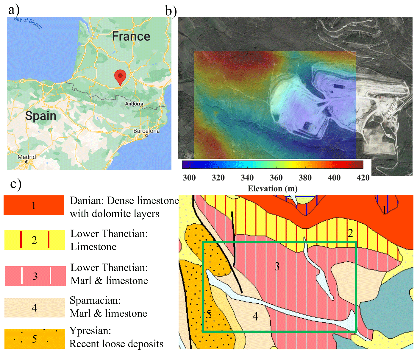
Figure 1 (a) Google map showing the location of the site (© Google Maps). (b) Obtained satellite view of the site superimposed with the elevation map of the area (© Google Earth). (c) The geological map of the area obtained from the French Geological Survey (© BRGM – https://infoterre.brgm.fr/, last access: 11 March 2024). The green box shows the boundaries of the acquisition area.

In the literature, DC estimation methods are usually categorized into multi-channel and two-station methods, even though there are no theoretical or significant technical differences between the two approaches (Papadopoulou, 2021). The multi-channel technique is the most common approach, in which the recordings from an array of receivers (in a 2D scheme) go through a wavefield transform (e.g., f−k, $f-v,$ and τ−p), and the DC is picked on the spectrum as the local maximum within the frequency band of surface waves. The multi-channel processing stage is repeated to estimate DCs at different locations, which are then inverted individually (e.g., fast simulated annealing of Beaty et al., 2002) or simultaneously (e.g., LCI of Socco et al., 2009) to estimate the V_s model. For SWT, DCs are estimated using the two-station processing method, in which the receiver couples aligned with sources are considered to estimate many path-averaged DCs that are later inverted using a tomographic scheme to estimate the V_s model directly (Boschi and Ekström, 2002; Fang et al., 2015; Boiero, 2009; Socco et al., 2014; Karimpour et al., 2022) or indirectly (Yoshizawa and Kennett, 2004; Shapiro and Ritzwoller, 2002; Yao et al., 2008).

Here, we show the application of the three surface-wave methods (W/D, LCI, and SWT) to estimate both V_s and V_p models. The first two methods are based on multi-channel DCs, whereas the latter relies on DCs from the two-station method. We apply the methods to a challenging test dataset that was acquired at a hard-rock site using the irregular source–receiver layout. The irregular source–receiver outline limits the use of conventional multi-channel processing methods. Conversely, the irregular combination of source–receiver is favorable for the estimation of many two-station DCs with different azimuthal angles, providing high data coverage and uniform azimuthal distribution of the paths, which is to SWT's advantage. The three surface-wave methods are customized for analyzing data with a low signal-to-noise ratio, which is often observed in collected data from hard-rock sites.

In this paper, we first introduce the site and describe the acquired data. Then, we explain the multi-channel and two-station DC estimation processing techniques. Then, we briefly describe the W/D, LCI, and SWT velocity model estimation methods and show their application to the dataset. We use the W/D method to estimate the a priori Poisson's ratio required by the LCI and SWT methods, which we then employ to transform their V_s results into V_p. Finally, we compare the estimated models and the obtained resolution from the application of each method and compare the methods from an efficiency point of view.

2 Site description and field dataset

The location is a limestone quarry in Aurignac in the south of France (Fig. 1a). In Fig. 1b, we show the satellite view of the site superimposed with the elevation map of the area. From north-west to south-east, a significant natural (outside the pits) and human-made (inside the pits) elevation contrast is present, which can cause highly scattered surface waves. In Fig. 1c, we show the geological map of the area from the website of the French Geological Survey (BRGM). The central, eastern, and northern parts of the site are characterized by stiff formations belonging to Thanetian and Sparnacian stages, primarily composed of stiff limestone and marl. In the western zone, recent loose deposits are present (Ypresian), creating a significant lateral variation between the east and west portions of the site. The very dense limestone with dolomite layers from Danian stage is outcropping in the north, outside of the investigated area, and is expected to be reached in shallow subsurface in the investigated zone.

Table 1 Acquisition parameters of the dataset for outside the mining pits.

The seismic campaign was conducted inside and outside the two open mining pits to test the irregular source–receiver layout acquisition technique at a hard-rock site and provide an exploration dataset to be used for testing different processing approaches. Altogether, 918 receivers were deployed on a regular grid (area of 1.7 km × 1 km), and several source points (1077) were considered along the access roads, resulting in a 3D large-scale acquisition layout. We used two Birdwagen Mark IV off-road carriers equipped with 24 t vibrators as the source. The vibration included a sweep of 24 s (3 to 110 Hz) with a 5 s listening time. The data were collected in real-time using the RT2 wireless system. In this study, we considered a portion of the data that were collected outside the mining pits. The full description of the acquisition parameters corresponding to this portion of the data is given in Table 1.

To minimize the effect of elevation contrasts (Fig. 1b), we split the data into two sub-datasets (north and south), each corresponding to an area with relatively flat topography. In Fig. 2, we show the acquisition layout, where different colors are used for each sub-dataset.

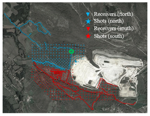
Figure 2 The satellite view of the Aurignac site (© Google Earth) superimposed with the acquisition layout. The data are divided into two sub-datasets shown with different colors, each within a relatively flat area. The recordings from the highlighted shot (green circle) are plotted in Fig. 3.

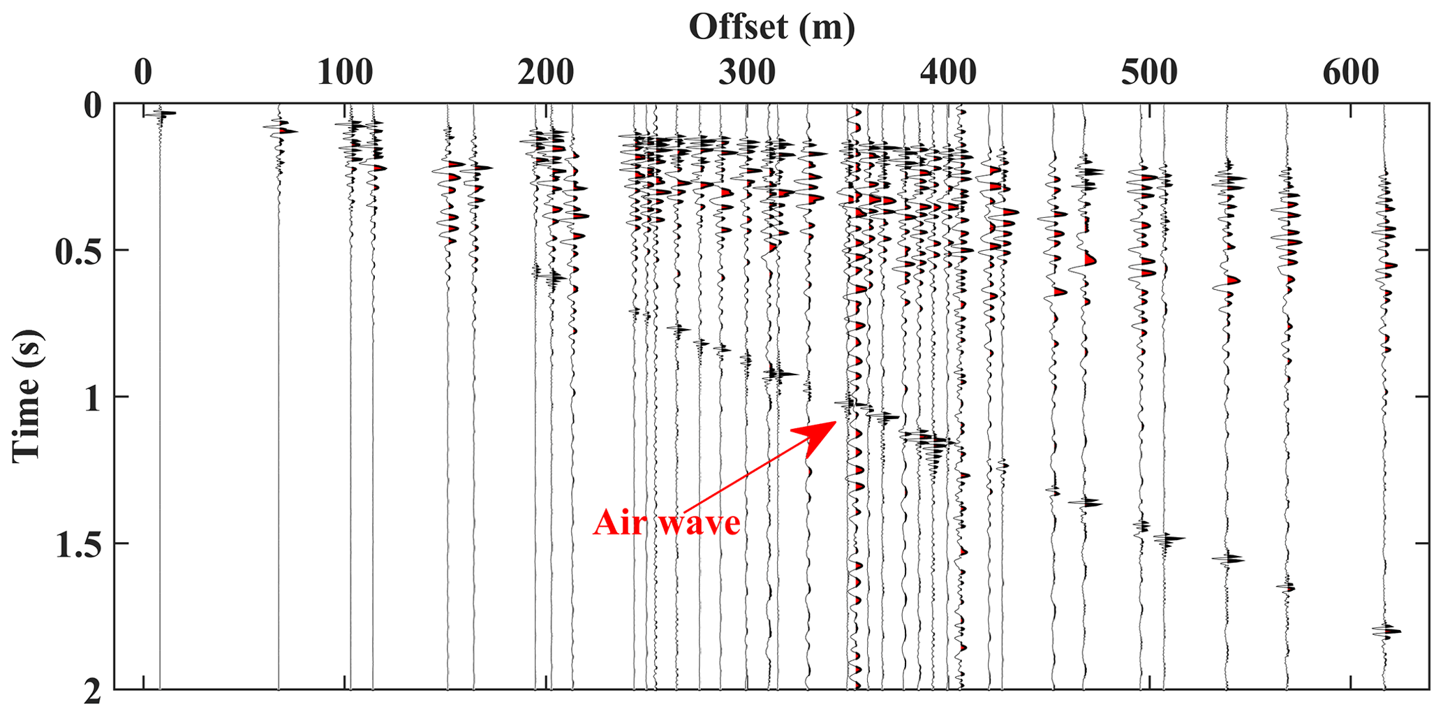
Figure 3 An example seismogram from the northern zone of the Aurignac site. The shot location is highlighted with a green circle in Fig. 2.

In Fig. 3, we show the first 2 s of the recordings from the highlighted source in Fig. 2 in the offset domain; only 20 % of the traces are shown for better visualization. The data exhibit a low signal-to-noise ratio as expected for hard-rock sites.

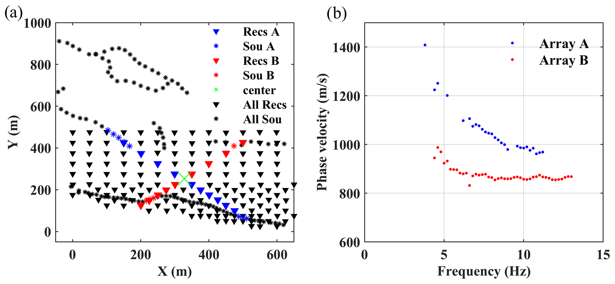
Figure 4 Two example DC estimations for the same location using two different receiver arrays. (a) The two receiver arrays and aligned shots. The middle of both arrays is coincident and shown with the green ×. (b) The estimated DCs for the location of the green × in a use of the two arrays' records.

3 Surface-wave processing of 3D data

3.1 Multi-channel DCs

Multi-channel dispersion analysis is usually performed by selecting recordings from multiple inline receivers with a source and performing domain transform (f−v, f−k, τ−p, etc.). Nevertheless, this approach can lead to inconsistencies in the estimated DCs when the technique is applied to 3D datasets with irregular source–receiver geometry at sites with significant lateral variations. In Fig. 4, we show two examples of DC estimation from the field dataset for the same location using recordings from two linear receiver arrays. The estimated DCs for the location shown as a green × in Fig. 4b differ on average by more than 15 %. The main reason for this inconsistency is the impact of lateral variations and the entirely different surface-wave propagation path along the two arrays.

To minimize the impact of lateral variability on the DC estimation of the 3D data, we consider the recordings from receivers spread over an area (Wang et al., 2015; Xia et al., 2009; Park, 2019). For each DC estimation, we select the receivers inside a square area (window) and consider the sources within a certain distance from the center of the square. We use the phase shift method (Park et al., 1998) to estimate the f−v spectrum. We stack the spectra corresponding to the recordings of the same receivers but from different source locations to increase the signal-to-noise ratio (Neducza, 2007). Then, the fundamental mode is picked as the maximum on the spectrum and is assigned to the center of the receiver spread. We slide the window by one inter-receiver spacing to estimate DCs corresponding to different locations of the site.

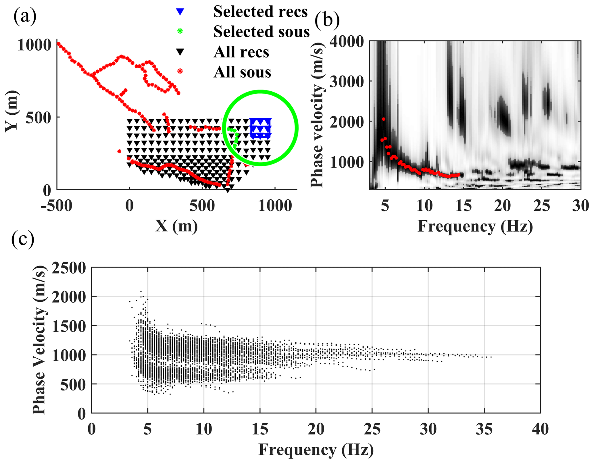
Figure 5 Multi-channel DC estimation from the field data. (a) An example geometry of the selected receivers and sources for DC estimation in the northern zone. (b) The computed spectrum and estimated DC from the recordings of the receivers shown in (a). (c) All the estimated DCs for the northern and southern zones.

For the field data, we considered a window of 100 m × 100 m to select the receiver and sources within 250 m of the center of the square. In Fig. 5, we show an example DC picking for the northern zone. In Fig. 5a, the nine selected receivers inside the square are shown in blue, and the selected shots are plotted in green asterisks. In Fig. 5b, we show the computed spectrum and the picked DC. Overall, we estimated 545 DCs for the northern and southern zones shown in Fig. 5c.

3.2 Two-station DCs

The two-station DCs are estimated applying interferometry to the recordings from receiver couples aligned with a source, assuming straight ray approximation. We use the algorithm developed by Da Col et al. (2020) and modified by Khosro Anjom et al. (2021). First, an automatic search is performed to find the receiver couples aligned with the source at each azimuth angle, considering 1° of tolerance for the deviation from a straight path. Given the scale of the site, we consider the propagation path as occurring over a plain area, and we neglect the great-circle approximation. Then, the traces are narrow-band filtered at various frequencies, using zero-phase Gaussian filters, and the filtered traces of the receiver couples are cross-correlated and assembled to form the cross-multiplication matrix. We use a third-order spline interpolator to convert the cross-multiplication matrix to the frequency–velocity domain. We stack the cross-multiplication matrices computed from the records of the same two stations, but different sources, to increase the signal-to-noise ratio. Finally, at each frequency, the phase velocity is picked as the maximum of the cross-multiplication matrix. To avoid cycle skipping, we use the closest multi-channel DC as a reference, and we automatically pick maxima closest to the reference DCs. To minimize the contamination of the fundamental mode by higher surface-wave modes, we damp the higher-mode data using the muting strategy of Khosro Anjom et al. (2019).

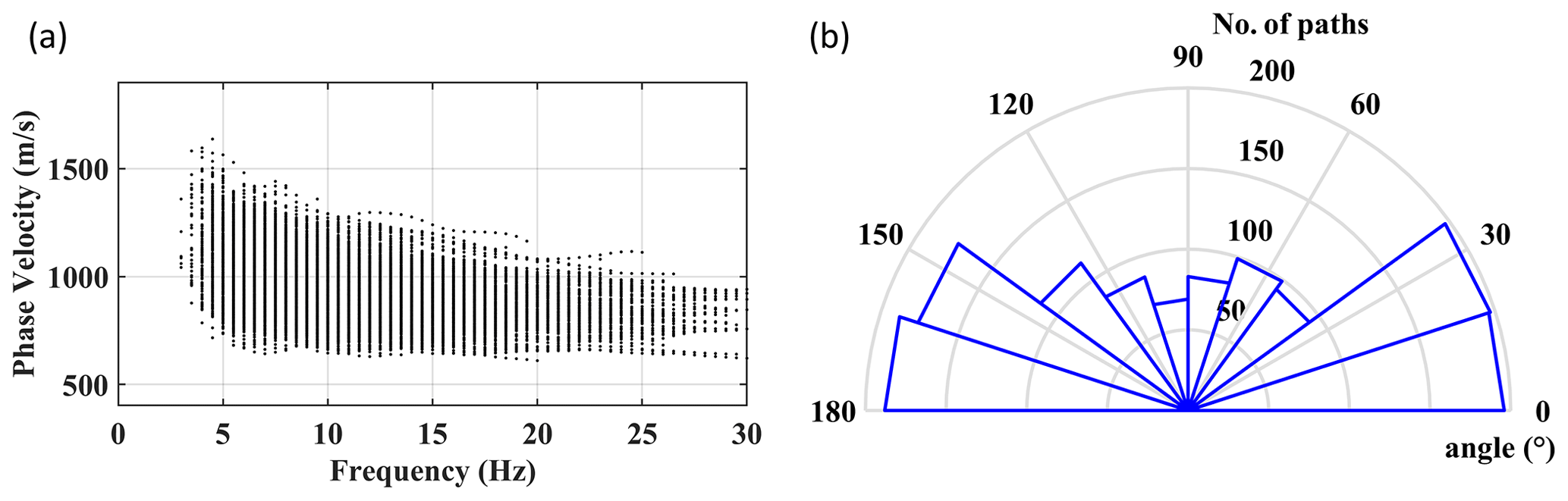
Figure 6 (a) The estimated path-averaged DCs corresponding to northern part of the site. (b) The obtained azimuthal illumination with the numbers around the great circle showing the angles and the other circles representing the obtained coverage.

We applied the two-station DC estimation method to the data from the north of the site only (blue markers in Fig. 2). We performed an automatic search of the receiver couples aligned with sources within a 250 m offset, which resulted in 4710 possible receiver couples and source settings. We used the local DCs from the multi-channel analysis (Fig. 5c) as references to locate the correct trend of the path-averaged fundamental-mode DCs. We discarded noisy or inconsistent cross-multiplication matrices, and, in total, 1301 path-averaged DCs were estimated. In Fig. 6a and b, we show the estimated path-averaged DCs and the observed azimuthal illumination. The data show uniform coverage with most paths showing angles between 0 to 40° and 140 to 180°. The uniform coverage mitigates the directionality of the tomographic inversion toward dominant directions (Khosro Anjom et al., 2021).

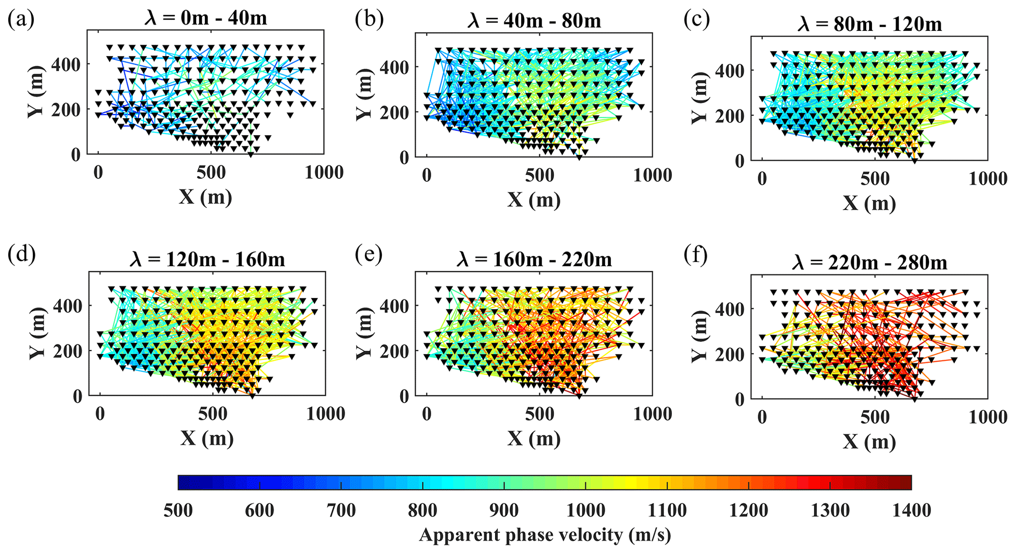
Figure 7 Pseudo-slices of the estimated path-averaged DCs from the north of the site shown within wavelength ranges of (a) 0 to 40 m, (b) 40 to 80 m, (c) 80 to 120 m, (d) 120 to 160 m, (e) 160 to 220 m, and (f) 220 to 280 m.

In Fig. 7a–f, we show the data coverage within different wavelength ranges, where the color scale shows the path-averaged phase velocity. The data exhibit very high coverage for wavelengths between 40 to 220 m, beyond which it decreases substantially.

4 Velocity model estimation

4.1 W/D data transform

The only inputs of the W/D method are the estimated multi-channel DCs. The method, as described in Khosro Anjom et al. (2021), is composed of four main steps: (i) the clustering of DCs, (ii) the selection of a reference DC for each cluster and the estimation of the corresponding time-average V_s velocity model, (iii) the W/D relationship and apparent Poisson's ratio estimation for the reference DC of each cluster, and (iv) the direct transformation of the DCs into time-average and then interval V_s and V_p models.

Since the same W/D relationship is applied to different DCs to transform them into velocity models, to apply the method at sites with significant lateral variations, the DCs must be clustered into more homogenous sets, and one W/D relationship should be estimated and applied separately to each cluster of DCs. We use the hierarchical clustering algorithm developed by Khosro Anjom et al. (2017) to cluster the DCs.

For each cluster, a reference DC and its corresponding time-average V_s model is needed to estimate the W/D relationship. The reference DC is selected based on the quality control proposed by Karimpour (2018). The time-average velocity is used in many applications, ranging from static correction of the reflection data to seismic hazard analysis, where the time-average velocity down to a depth of 30 m, the so-called V_s30, is used as a proxy for seismic response classification. To estimate the required time-average V_s model, we invert the reference DC using an optimized Monte Carlo inversion (Socco and Boiero, 2008). The density has a minor impact on the surface-wave velocity (Xia et al., 1999; Foti and Strobbia, 2002) and is defined a priori based on the geological information about the site. The V_s, the Poisson's ratio, and the thicknesses are randomly sampled within the boundaries of a wide, uniform model space. Then, the synthetic DCs corresponding to each model are computed and compared with the experimental DC. The algorithm uses the scaling properties of DCs to create an optimal model space based on the initial model space: before computing the misfit with the experimental DC, the synthetic DCs of the random models are shifted as close as possible to the experimental DC, then the scaling factor is obtained from the DC shift and is used to scale the models. These scaling steps, which are performed in a fully automatic manner, highly optimize the model space sampling that is focused on low-misfit regions and reduce the number of required simulations. Unlike deterministic inversions that result in a single output, the Monte Carlo inversion leads to a set of possible solutions. The best-fitting models are selected according to a one-tailed Fisher's test, imposing a certain level of confidence. Then, the selected layered V_s models are transformed to time-average V_s models using Eq. (1). The values of the selected time-average V_s models are averaged at each depth to obtain a unique time-average V_s model corresponding to the reference DC. Next, we estimate the W/D relationship that consists of the pairs of wavelength and depth values for which the phase velocity of the DC and the time-average V_s of the Monte Carlo solution have the same value. Comprehensive synthetic and real data analyses have been performed by Socco et al. (2017), Khosro Anjom et al. (2019), and Khosro Anjom (2021) to show the high sensitivity of the W/D relationship to Poisson's ratio. We use the method of Socco and Comina (2017) to estimate from the experimental W/D relationship an apparent Poisson's ratio that relates the time-average V_s and the time-average V_p. First, we generate synthetic DCs corresponding to the estimated V_s model from the Monte Carlo inversion and different Poisson's ratios. Then, we consider these DCs and the time-average V_s to retrieve synthetic W/D relationships that are each corresponding to a specific Poisson's ratio value. Next, we deduce an apparent Poisson's ratio at each depth by comparing the experimental W/D relationship with the synthetic ones. The estimated Poisson's ratio is an apparent one that relates time-average V_s and V_p of the cluster (Khosro Anjom et al., 2019).

We use the estimated experimental W/D relationship to directly transform all DCs of the cluster into time-average V_s models. Then, we transform the estimated time-average V_s models into time-average V_p through the estimated apparent Poisson's ratio. The time-average velocities can be transformed to interval velocities using a Dix-type equation. In order to reduce the impact of noise in the data, we employ the regularized Dix-type formulation suggested by Khosro Anjom (2019) to convert the time-average V_s and V_p models into interval V_s and V_p. It is important to emphasize that the estimated models are not layered velocity models but rather interval velocity models with 1 m intervals for the entire investigation depth. Finally, we assemble all the estimated models from the clusters to build a pseudo-2D/3D model.

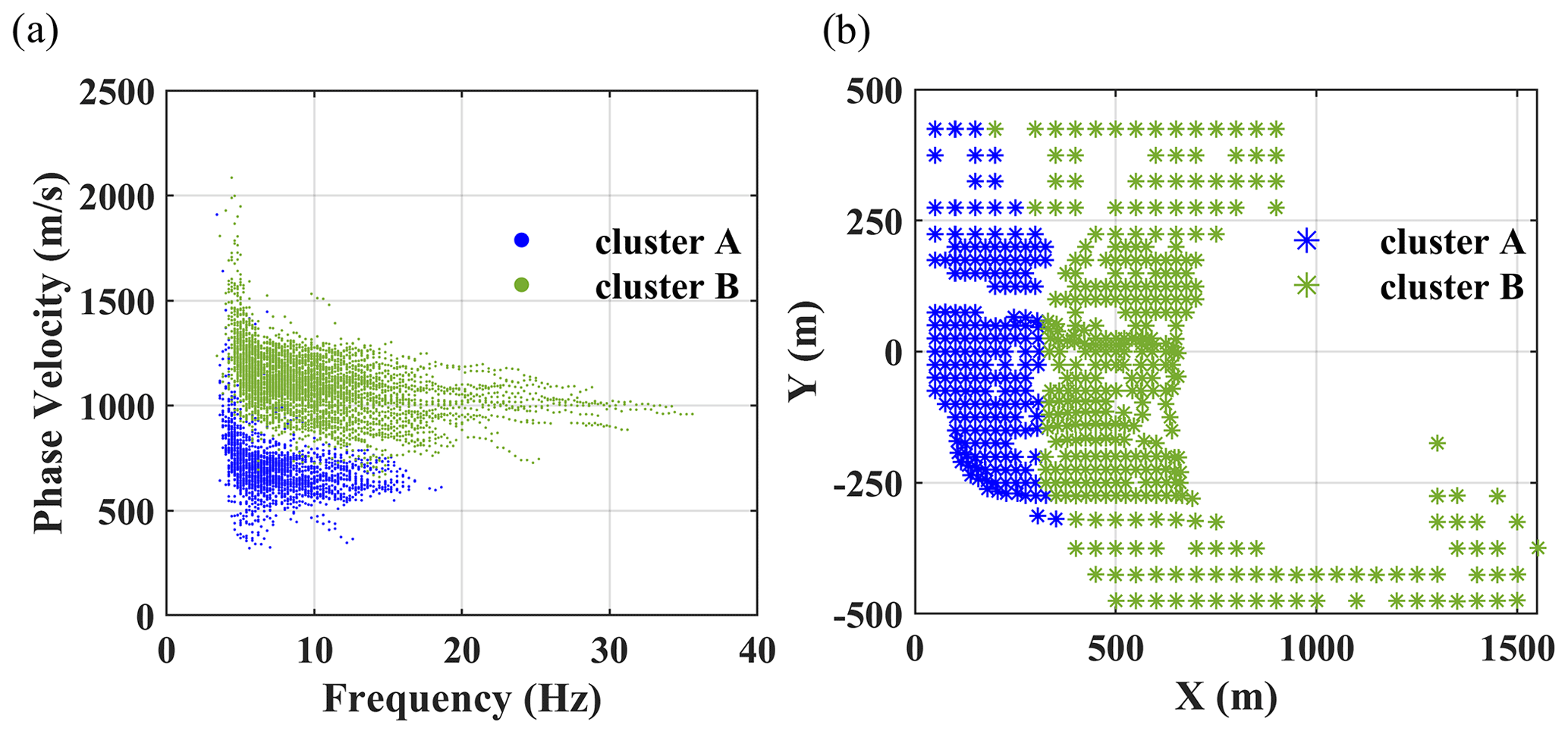
Figure 8 Clustering of the multi-channel DCs. (a) The estimated DCs. (b) The spatial view of the estimated DCs and obtained clusters.

4.2 LCI

The method's inputs are the multi-channel DCs and the initial models at the location of the local DCs. An initial model defined as the thickness, density, Poisson's ratio, and V_s is set for each cluster of DCs. The thickness and V_s are based on the Monte Carlo inversions of reference multi-channel DCs in Sect. 4.1. The Poisson's ratio is selected based on the W/D analysis. We use information from the site to define the densities of the model.

The inversion method is a deterministic least-squares inversion based on Auken and Christiansen (2004), which was developed by Boiero (2009) and modified by Khosro Anjom (2021) to support parallel computing. At each iteration the V_s and thicknesses are updated, and the Poisson's ratio and density are fixed a priori. All the DCs are inverted simultaneously for a set of 1D models that are tied by lateral constraints between parameters of neighboring models. We use a damped least-squares inversion scheme (Marquart, 1963) with lateral constraints (Auken and Christiansen, 2004) to update the model iteratively. The constraints act as spatial regularization, and their strength is defined to avoid both overfitting and over-smoothing. Weak lateral constraints or lack of lateral constraints can create unrealistic lateral changes in the final model, whereas constraints that are too strong can result in an over-smoothed model, masking the sharp lateral variations in the site. We use the data misfit as an indicator for choosing the level of constraints: the inversion with the highest level of constraint that does not impact the DC misfit compared to unconstrained inversion is selected. A thorough description of the method is available in Boiero (2009) and Socco et al. (2009), and the strategy for constraint selection is provided in Boiero and Socco (2010).

4.3 SWT

The inputs of the tomographic inversion are the path-averaged DCs from the two-station method and the initial model. The parameters of the initial model are the thickness, V_s, Poisson's ratio, and density. The model points are defined with equal distances in X and Y directions. The distance of the model points depends on the required resolution and also on the data coverage (i.e., path-averaged DCs). The parameters of the initial model are selected the same as the initial model of LCI (Sect. 4.2).

We use the tomographic inversion algorithm developed by Boiero (2009) and modified by Khosro Anjom et al. (2021). An essential part of the tomographic inversion is the computation of synthetic path-averaged DCs corresponding to the observed ones. We compute the path-averaged DCs, assuming a straight ray path approximation between the two receivers and as reciprocal of the average slowness along the paths discretized over the model grid. The phase velocities at the location of the discretized paths are computed by bi-linear interpolation of the phase velocities from local DCs corresponding to the adjacent model points (Boiero, 2009).

Similar to the LCI algorithm, a damped least-squares method (Marquart, 1963) with lateral constraints is used to iteratively update the model until the minimum misfit between synthetic and observed DCs is reached. The only parameter that updates in the inversion is V_s, while the others are fixed a priori. This method allows the implementation of lateral constraints. We consider the same criteria explained in Sect. 4.2 to select the optimal constraint level. In contrast with the other two methods, the SWT method is applied to the northern dataset only due to computational capacity restrictions that will be explained in the Discussion (Sect. 6).

5 Results

5.1 W/D data transform

The clustering of all the estimated DCs generated two clusters. In Fig. 8a, we show the estimated DCs with the color scale based on the clustering of the DCs in Fig. 8b. The DCs of the western cluster (cluster A, shown in blue in Fig. 8a) present lower phase velocities compared to the eastern DCs (cluster B, shown in green in Fig. 8a).

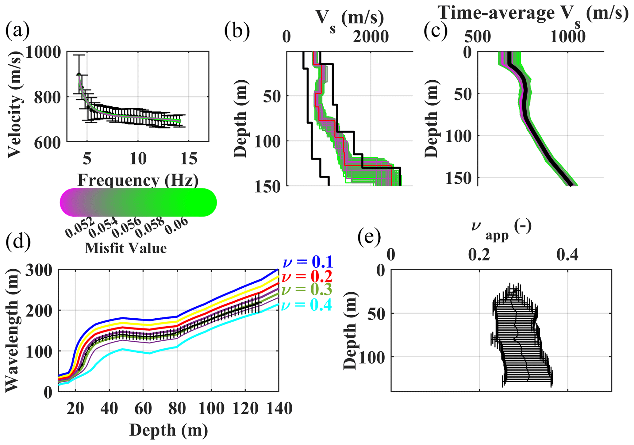
Figure 9 The steps of estimating the reference W/D relationship and apparent Poisson's ratio for cluster A. (a) The reference DC with the phase velocity and uncertainty and the synthetic accepted DCs from the Monte Carlo inversion. (b) The accepted V_s models from the Monte Carlo inversion, where the black lines show the initial boundaries of the model space. (c) The accepted time-average V_s models from the Monte Carlo inversion. In black, the reference time-average V_s. (d) Estimated reference W/D relationship. The colored W/D relationships are the synthetic ones, each with a constant Poisson's ratio, used for apparent Poisson's ratio estimation. (e) The estimated reference apparent Poisson's ratio.

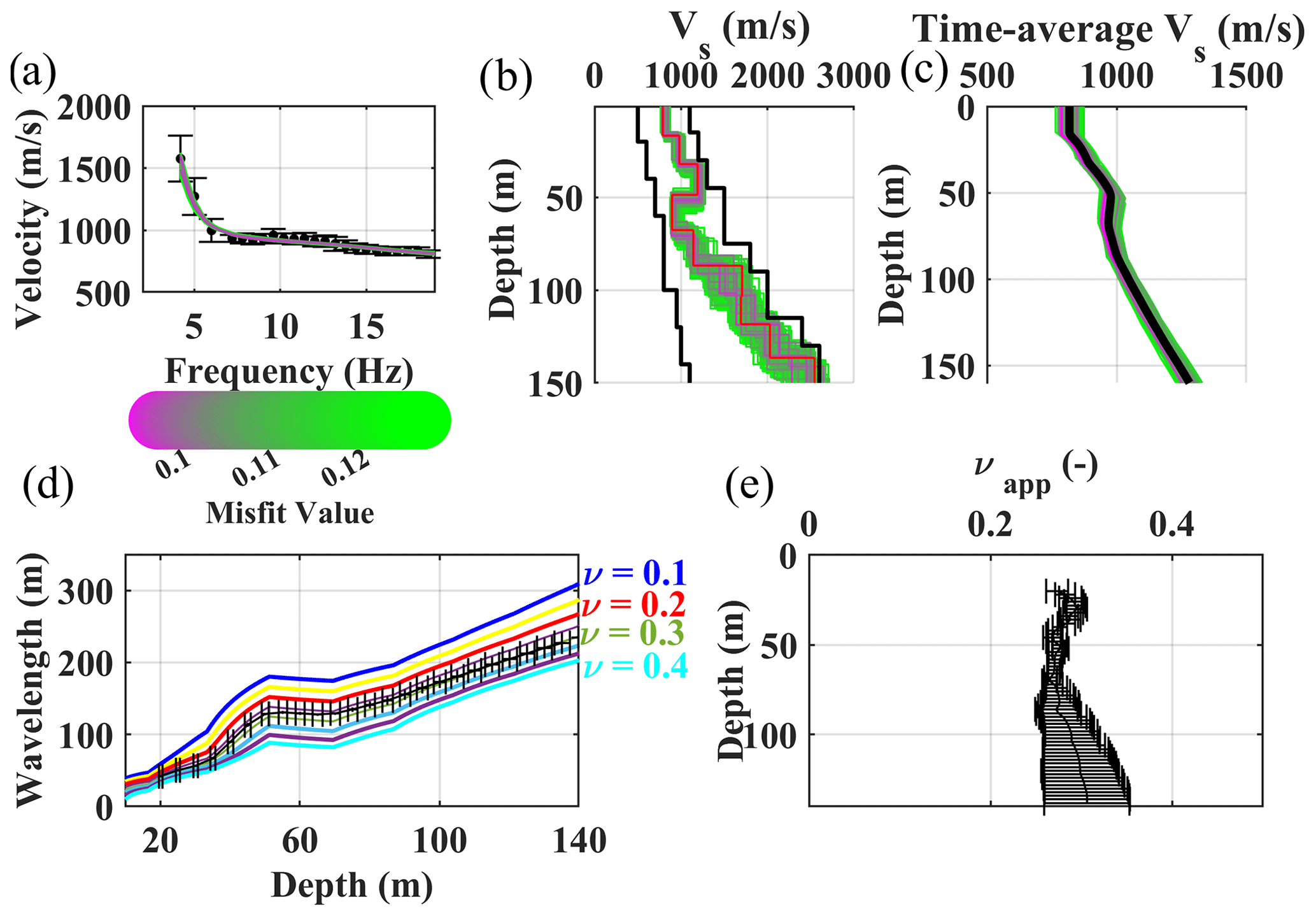
Figure 10 The steps of estimating the reference W/D relationship and apparent Poisson's ratio for cluster B. (a) The reference DC with the phase velocity and uncertainty and the synthetic accepted DCs from the Monte Carlo inversion. (b) The accepted V_s models from the Monte Carlo inversion, where the black lines show the initial boundaries of the model space. (c) The accepted time-average V_s models from the Monte Carlo inversion. In black, the reference time-average V_s. (d) Estimated reference W/D relationship. The colored W/D relationships are the synthetic ones, each with a constant Poisson's ratio, used for apparent Poisson's ratio estimation. (e) The estimated reference apparent Poisson's ratio.

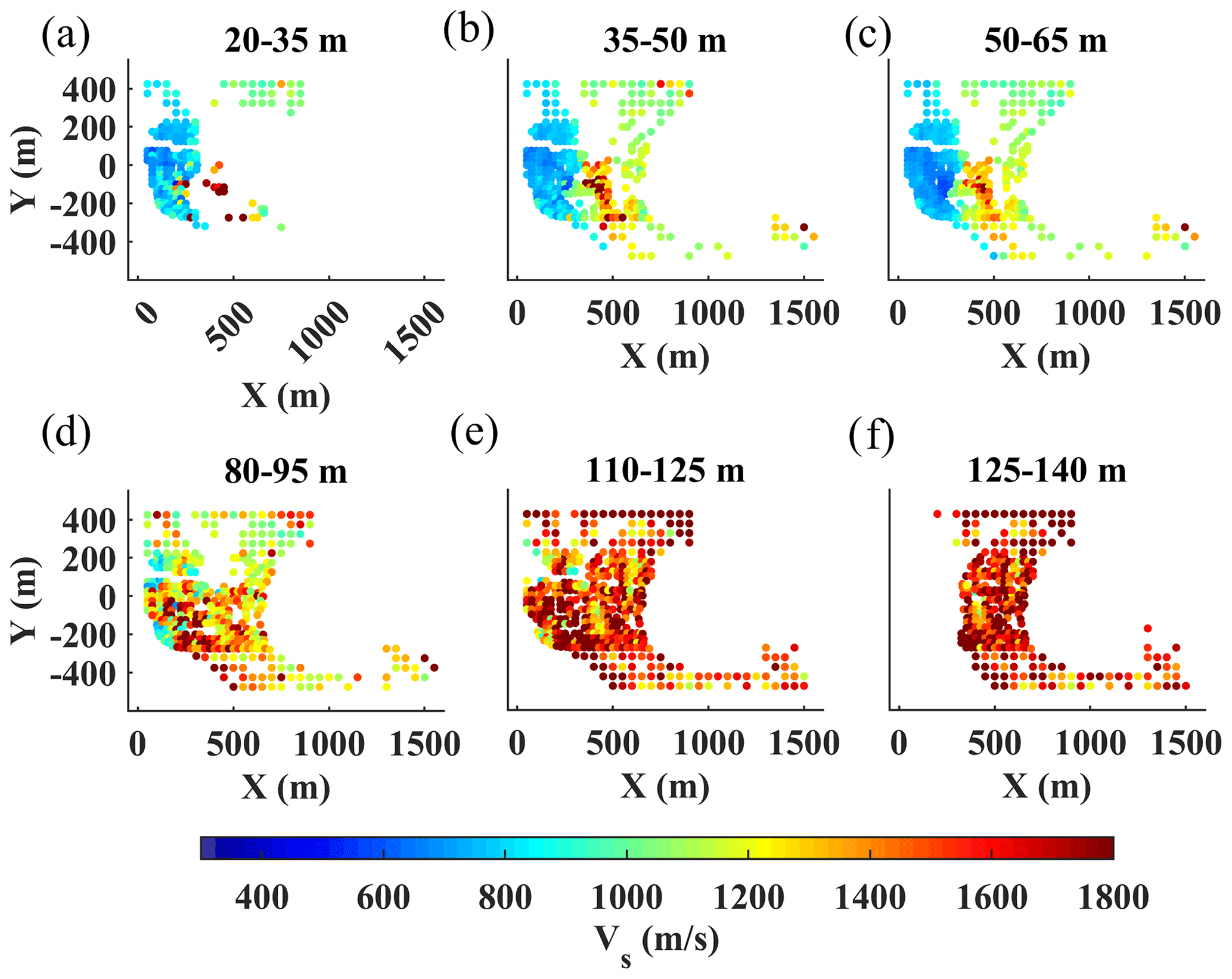
Figure 11 The estimated V_s model using the W/D method. (a–f) The horizontal slices at the different depth intervals indicated on top of each plot.

In Figs. 9 and 10, we show the steps of estimating the reference W/D relationship and apparent Poisson's ratio for the reference DCs of clusters A and B. We considered variable Poisson's ratios between 0.1 and 0.45 for the Monte Carlo inversion. Based on the information from the site, we considered density of 2000 kg m⁻³ for the first layer and constant density of 2200 kg m⁻³ for the other layers. We imposed a 0.001 level of confidence for the Fisher's test to accept the best-fitting models among 1 million sampled models. In Fig. 9b and c, as well as Fig. 10b and c, we show the estimated V_s and time-average V_s models for clusters A and B, respectively. In Figs. 9b and 10b, we also show the boundaries of the V_s model space for the Monte Carlo inversion. Due to the application of the scale properties, the selected models can be scaled to outside of the original boundaries of the model space (Socco and Boiero, 2008). The estimated W/D relationships for clusters A and B are shown in Figs. 9d and 10d, whereas the obtained apparent Poisson's ratios are provided in Figs. 9e and 10e. In Fig. 9d and e, as well as Fig. 10d and e, we also show the uncertainty associated with the reference W/D and with the apparent Poisson's ratio of the clusters, which was obtained based on the method of Khosro Anjom et al. (2019).

For both clusters, the W/D relationship and apparent Poisson's ratio were not available for the first 20 m due to the lack of short-wavelength data in the experimental DCs. The investigation depth of 128 m was reached for cluster A, whereas this value was increased to 140 m for cluster B.

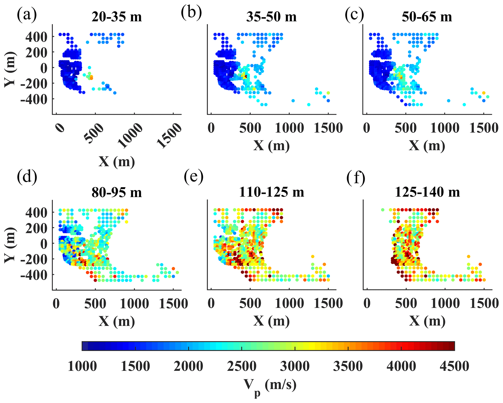
Figure 12 The estimated V_p model using the W/D method. (a–f) The horizontal slices at the different depth intervals indicated on top of each plot.

The estimated DCs from the two clusters were transformed to interval V_s and V_p models using the reference W/D relationships and apparent Poisson's ratios (Figs. 9d, e and 10d, e). In Fig. 11, we show several horizontal slices of the estimated V_s model averaged over the depth intervals indicated on top of each plot. Similarly, in Fig. 12, we show the horizontal slices of the estimated V_p averaged over the same depth intervals. Both models show a sharp velocity transition between the eastern and western sides of the area at shallow depths above 65 m (Figs. 11a–c and 12a–c). This contrast is created by the transition from the high-velocity limestone and marl formations in the east to the loose materials characterized by lower velocity in the west. Below 110 m (Figs. 11e, f and 12e, f) the contrast disappears, reaching the high-velocity formation probably from the Danian stage.

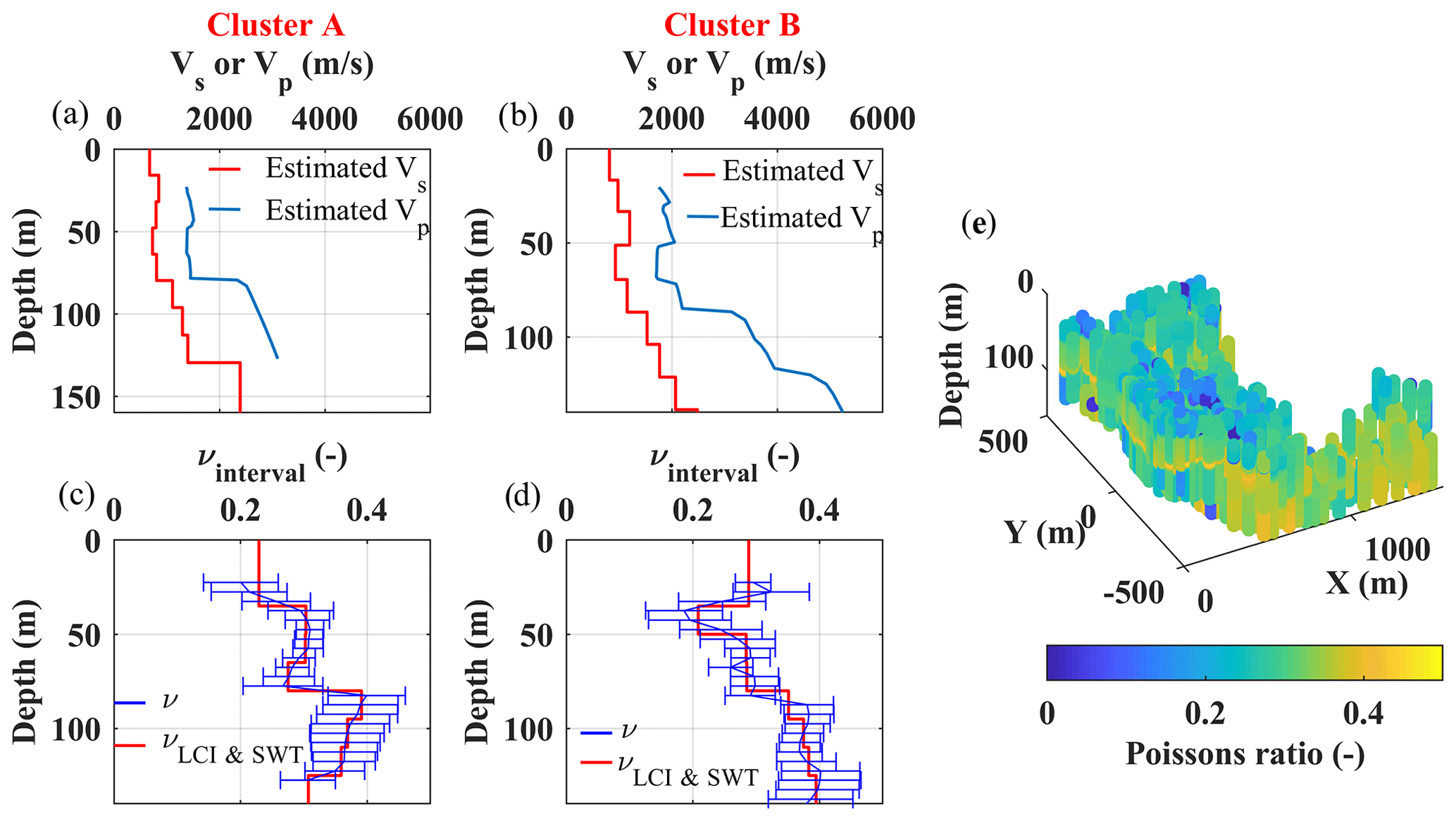
Figure 13 Poisson's ratio estimation for clusters A and B. (a, b) The estimated V_s and V_p models corresponding to the reference DCs of clusters A and B. (c, d) In blue, the estimated Poisson's ratios for clusters A and B. In red, the averaged and extrapolated Poisson's ratio corresponding to the layers of LCI and SWT. (e) The 3D view of the obtained Poisson's ratios from the estimated V_s and V_p models of the W/D method in Figs. 11 and 12.

5.2 LCI

We defined an initial model composed of nine layers overlying a half-space with constant thicknesses of 15 m, except for the first layer, which was set at 20 m, giving an investigation depth of about 140 m. We assigned the Poisson's ratios of the model based on the results of the W/D analysis: using the estimated V_s and V_p models at the reference location of each cluster (Fig. 13a and b), we obtained the Poisson's ratios, shown in Fig. 13c and d (in blue), corresponding to clusters A and B, respectively. Since the Poisson's ratios are assumed invariant within each cluster, we used all estimated Poisson's ratios of each cluster from the W/D method (Fig. 13e) to obtain an uncertainty for the estimated Poisson's ratios at each depth. The horizontal error bars in Fig. 13c and d show the standard deviation of the estimated Poisson's ratios. We averaged and extrapolated the values of the Poisson's ratio to match them with the layers of the LCI model (red lines in Fig. 13c and d). Based on the clustering analysis of the W/D method (Fig. 8b) and location of the LCI model points, we assigned the appropriate Poisson's ratio to each 1D model. We defined a constant density of 2200 kg m⁻³, except for the first layer (2000 kg m⁻³), based on the geological formations in the area.

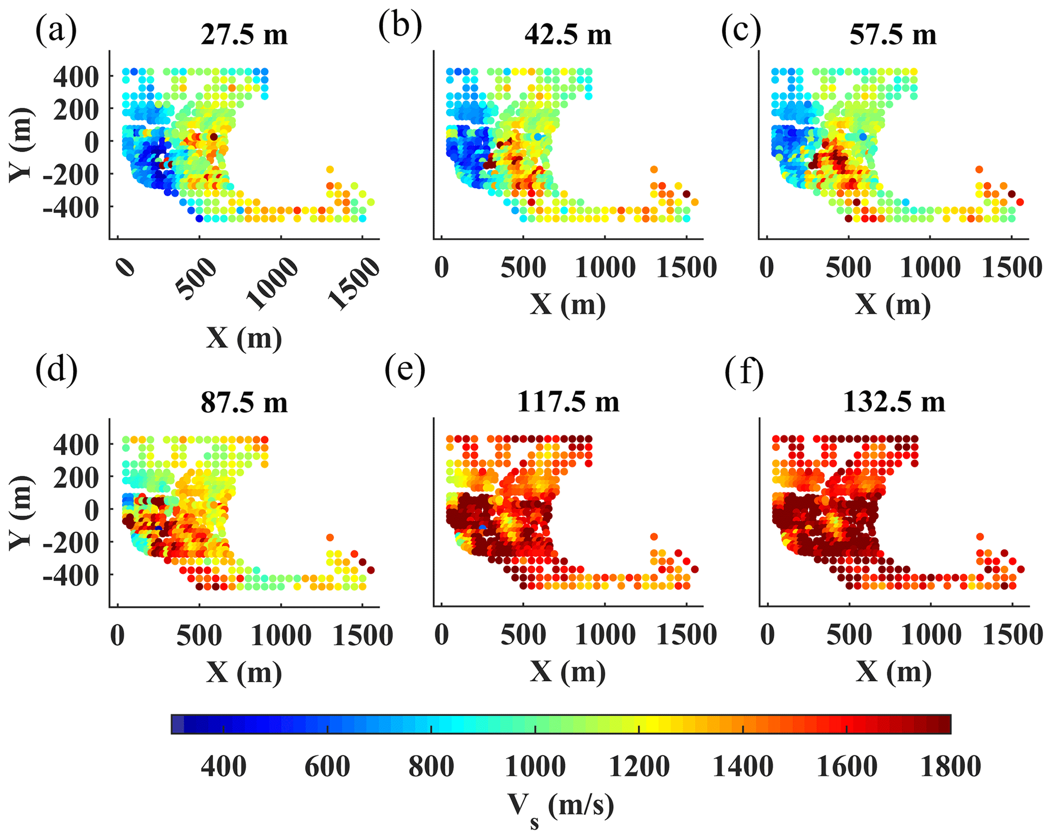
Figure 14 The estimated V_s model using the LCI method. (a–f) The horizontal slices at the different depths indicated on top of each figure.

We performed an unconstrained and several laterally constrained inversions to find the optimal level of constraints according to the strategy described in Boiero and Socco (2010). We chose a lateral constraint on V_s equal to 50 m s⁻¹, which was the highest level of constraints that did not significantly impact the inversion's residual misfit. The unconstrained inversion yielded a least-squares weighted misfit of 23.4, whereas the selected constrained inversion resulted in a misfit of 23.9. In Fig. 14, we show the horizontal slices of the estimated V_s model at various depths. Even though the inversion is laterally constrained, the algorithm was able to depict a sharp transition between the east and the west (Fig. 14a–c), which is in line with the results of the W/D method (Fig. 11a–c). The LCI model below 87.5 m shows high velocities with insignificant variations between east and west.

5.3 SWT

Given the high data coverage from the estimated path-averaged DCs (Fig. 7), we defined a dense model grid on the considered northern zone, composed of 300 1D models, aiming at obtaining a high-resolution model. We used the same initial models defined for LCI (Sect. 5.2).

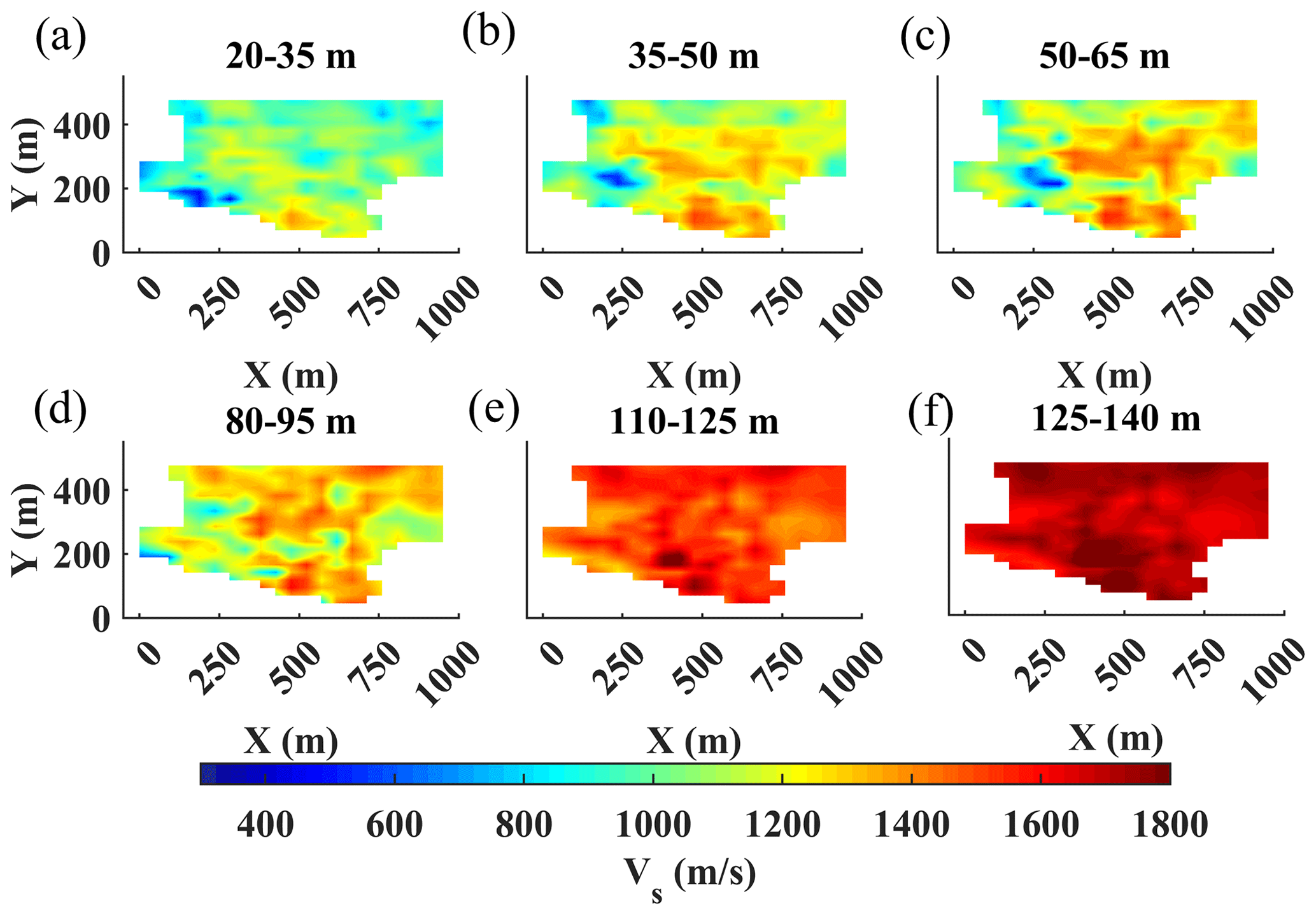
Figure 15 The estimated V_s model for the north of the site using the SWT method. (a–f) The horizontal slices at the different layers indicated on top of each figure.

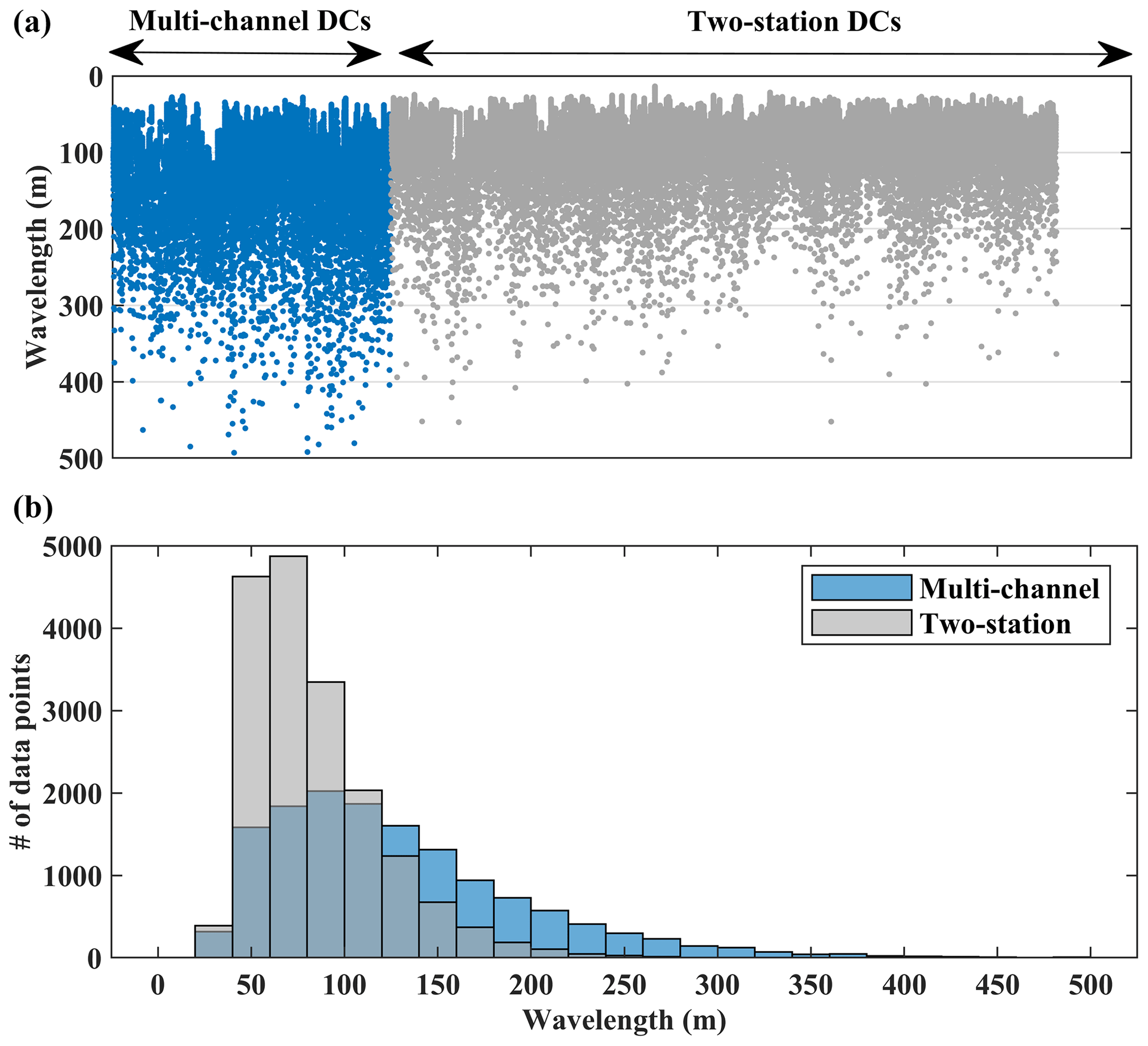
Figure 16 Comparison between the wavelength distributions of the multi-channel and two-station dispersion data. (a) The distribution of the wavelength shown separately for each estimated DC. (b) The histogram showing the wavelength distribution of all DCs within 20 m wavelength bins.

In Fig. 15, we show the estimated V_s at the different layers, which corresponds with the depth intervals defined for the estimated V_s of the W/D method (Fig. 11). We chose a lateral constraint of V_s equal to 50 m s⁻¹, which was the highest level of constraints that did not significantly impact the inversion's residual misfit. The unconstrained inversion yielded a least-squares weighted misfit of 42.1, whereas the selected constrained inversion resulted in a misfit of 43. Similar to the estimated model from W/D and LCI, the estimated model from SWT shows a significant velocity contrast between the east and the west. Nevertheless, this contrast is smoother than the other two models. This model shows high velocities with no significant lateral variation below a depth of 110 m, an indication of reaching the high-velocity limestone and marl formation from the Danian stage (Fig. 1c).

6 Discussion

We showed the application of three surface-wave methods for V_s model estimation, out of which the W/D and LCI methods provided the velocity models at the location of DCs, both in the northern zone (174 locations) and the southern zone (371 locations). The W/D method provided the V_p model and the reference Poisson's ratios used in LCI and SWT. SWT was applied only to the northern zone, which provided the V_s models at 300 defined model points. Here, we further evaluate the results of the three methods in terms of vertical resolution, spatial resolution, differences of the estimated models, and computational efficiency of each method.

In Fig. 16, we show the wavelength distribution of the estimated multi-channel DCs in blue, which shows dense data sampling up to wavelengths of 300 m, suggesting good vertical resolution also in deeper portions. These DCs were obtained from the recordings of receivers spread over a square window of 100 m × 100 m. The receiver window was shifted by one receiver spacing (50 m in the north and 25 m in the south). Neglecting the smoothing effect of superimposed receiver windows, the shifting distance can be considered as the spatial resolution of the multi-channel DC data.

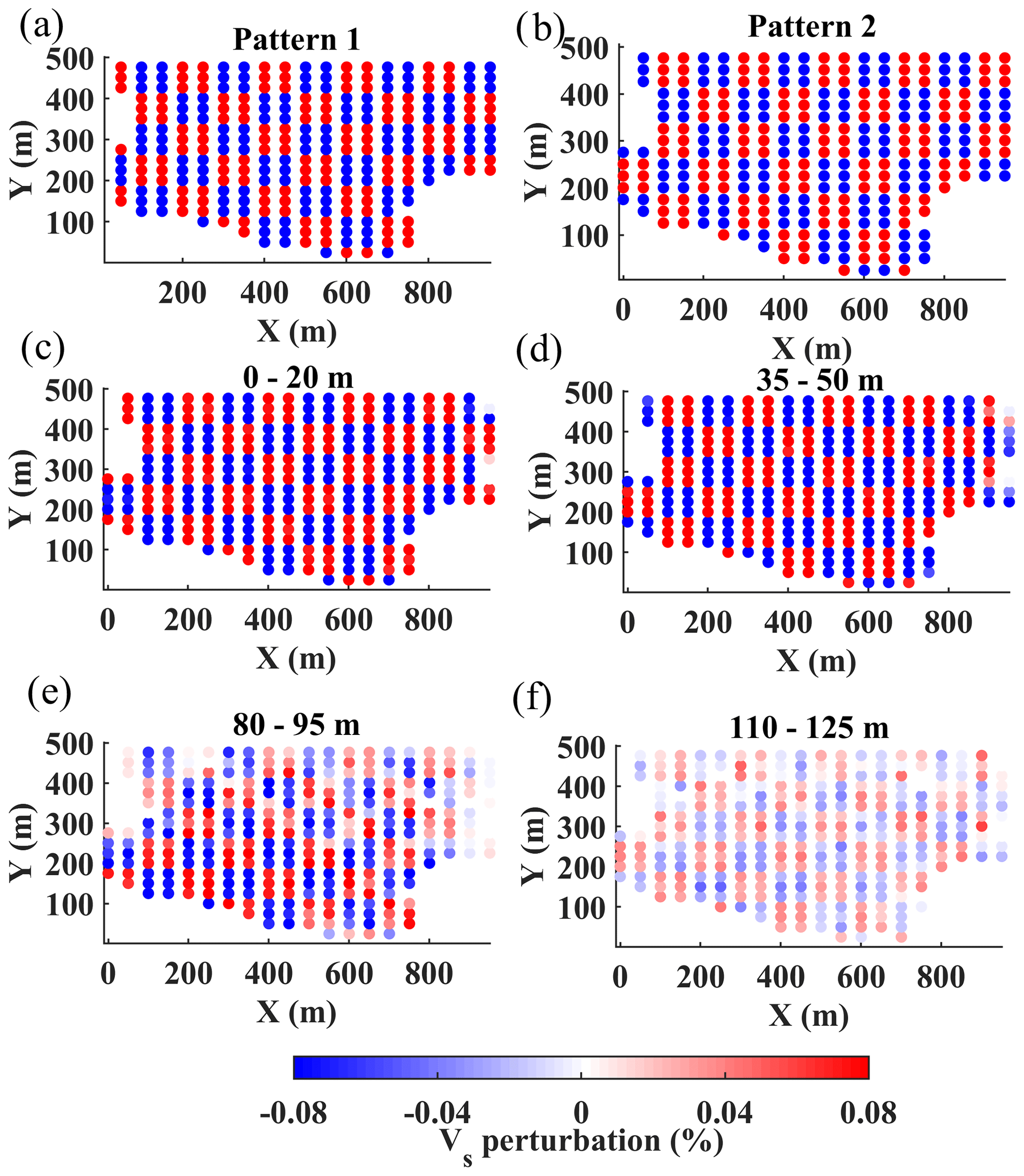
Figure 17 Checkerboard test. (a) Pattern 1, used to perturb V_s of layers 1, 2, 5, 6, and 9. (b) Pattern 2, used to perturb V_s of layers 3, 4, 7, and 8. (c) 0 to 20 m. (d) 35 to 50 m. (e) 80 to 95 m. (f) 125 to 140 m. The circles in the checkerboard test match the original dense grid used for the tomographic inversion of the real data.

In Fig. 16, in gray, we also show the wavelength distribution of the estimated two-station DCs. Even though the total number of DCs from the two-station analysis (1301) is far more than from the multi-channel analysis (545), the large wavelength data points (> 120 m) are sparser than the ones obtained with the multi-channel method (top plot in Fig. 16), mainly due to the low signal-to-noise ratio of cross-multiplication matrices at low frequencies. This shows that multi-channel DC analysis provides greater investigation depth compared to the two-station method. To mitigate the lack of investigation depth of SWT, we employed the wavelength-based weighting developed by Khosro Anjom et al. (2021) to increase the score of large-wavelength data points in the tomographic inversion, aiming at enhancing the resolution at depth. We performed a checkerboard test to evaluate the horizontal and vertical resolution of SWT. We perturbed the estimated V_s model from the SWT method (Fig. 15) by 8 % negatively and positively, which alternated every two layers (Fig. 17a and b). In Fig. 17c–f, we show the results of the inversion at various layers. The inversion is effective at all considered depths and across the whole model. The 50 m × 50 m perturbations were well-recovered up to depths of 50 m (Fig. 17c and d), providing similar spatial resolution compared to the LCI and W/D methods. The resolution slightly decreases towards the deepest portion of the model (Fig. 17e and f), especially in the northern part where long-wavelength data are lacking (Fig. 13f). It is noteworthy to mention that the location of the circles in Fig. 17 matches the model grid used for the tomographic inversion of the real data (Fig. 15).

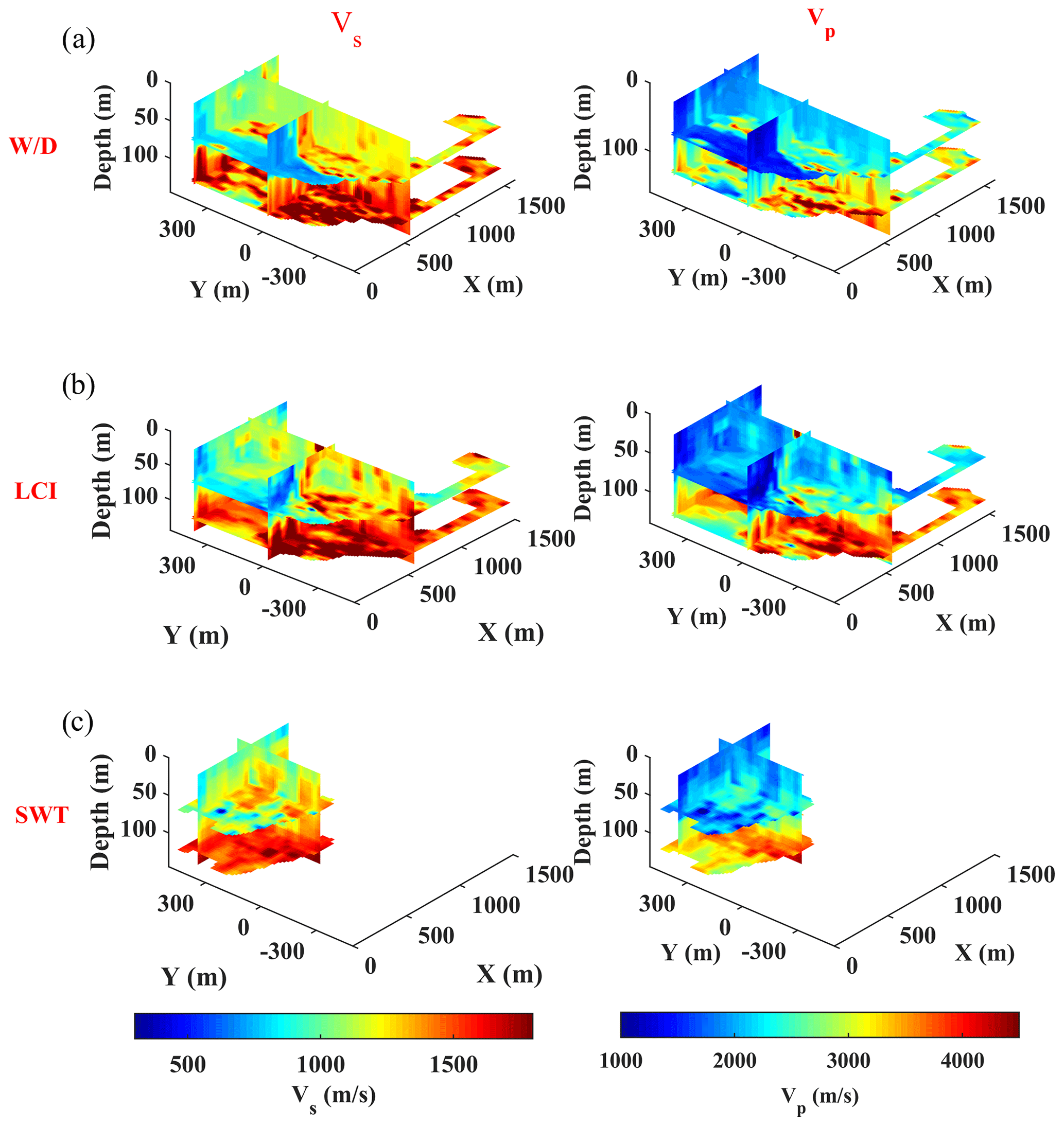
Figure 18 Isosurfaces of the estimated V_s models (left panels) and V_p models (right panels) using (a) W/D, (b) LCI, and (c) SWT methods. The sections are at plains x = 600 m, y = 0 and 400 m, and z = 70 and 125 m.

The application of the W/D method to the dataset provided both V_s and V_p models. We considered the estimated Poisson's ratio of the two clusters as prior information in the reference model of the LCI and SWT methods. Now, we use the same Poisson's ratios to transform the V_s results of these two methods to V_p models. We also linearly interpolate the V_s and V_p results from all three methods to obtain the velocity models at common voxels of 10 m × 10 m × 0.1 m within x, y, and z (depth) directions, respectively. In Fig. 18, we compare the retrieved pseudo-3D V_s and V_p models from the three methods at various isosurfaces. A very similar trend of variations for V_s (Fig. 18a–c) and V_p (Fig. 18d–f) is obtained from the application of the methods, and they all depict a significant variation between the eastern and western sides of the site.

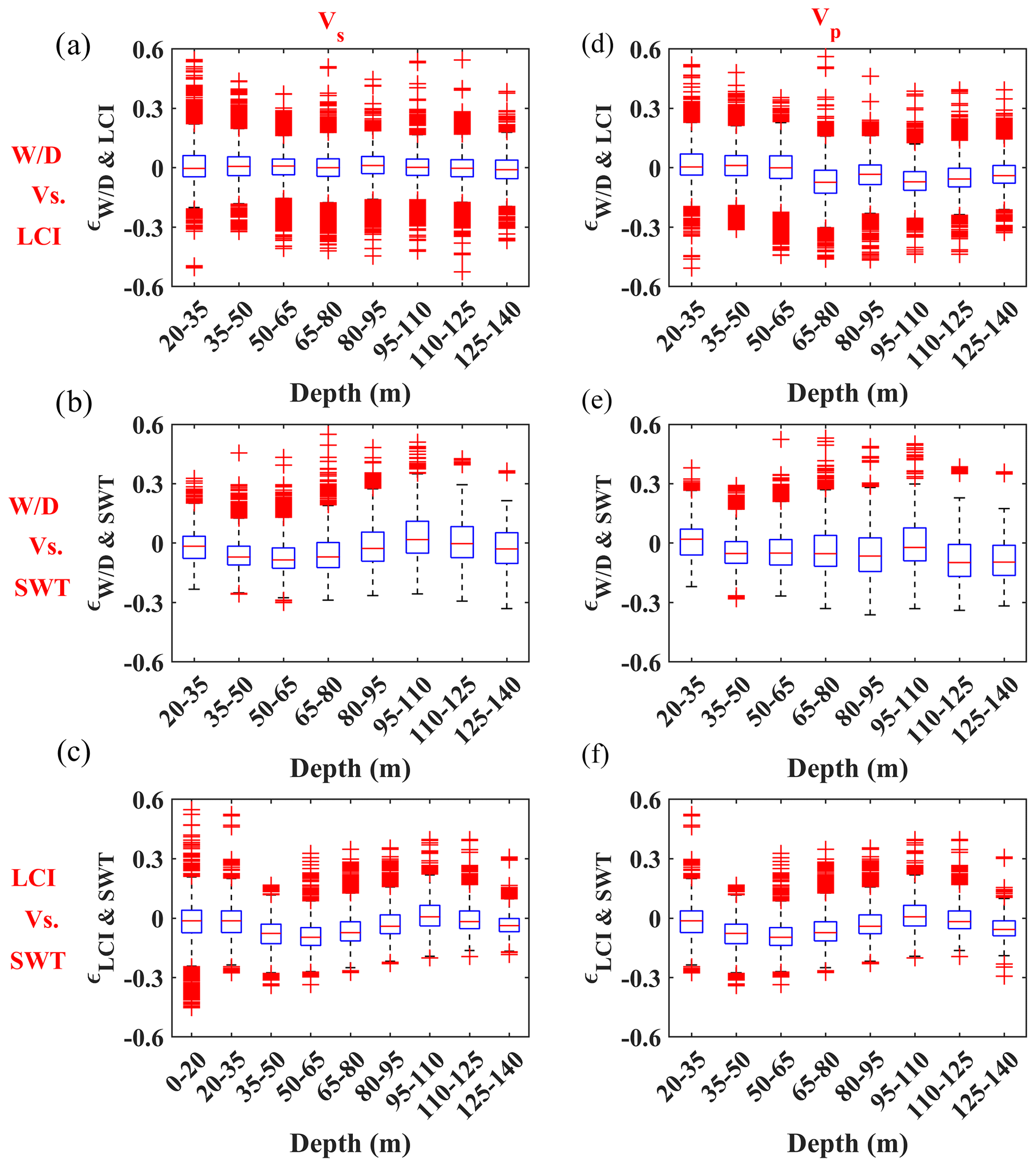
Figure 19 The box plot showing the difference between the V_s (a–c) and V_p (d–f) models obtained from the three methods computed using Eq. (2). The box plot is defined by three lines showing the 25th percentile, median, and 75th percentile of the residual's distribution and by whisker lines extending from the box's edges up to 1.5 times the distance between the edges of the box. The rest of the data are regarded as outliers and are shown with “+”. The box plots show the differences between the models obtained from (a) W/D and LCI, (b) W/D and SWT, and (c) LCI and SWT.

To compare the estimated models from each method quantitatively, we compute the difference between the estimated V_s and V_p of every two methods separately as

$$\begin{array}{}\text{(2)}& \mathit{\epsilon }(i,j,k)=\mathrm{2}\times \left[{\displaystyle \frac{V(i,j,k{)}_{\text{method.1}}-V(i,j,k{)}_{\text{method.2}}}{V(i,j,k{)}_{\text{method.1}}+V(i,j,k{)}_{\text{method.2}}}}\right],\end{array}$$

where i, j, and k are the indices of the voxels in x, y, and z (depth) directions, respectively, and V is the velocity. In Fig. 19, we show the boxplots of the differences compartmentalized within different depth intervals. The differences are computed for depths between 20 and 140 m, except for the V_s comparison of LCI and SWT (Fig. 19e), which also includes the first 20 m. This is due to the lack of short-wavelength data for the W/D method. The significant registered differences (red “+”) are mainly caused by the methods' different parameterizations in depth: the W/D method provided continuous velocities in depth (every 10 cm), while SWT and LCI provided layered models. Although we defined similar reference models for the LCI and SWT methods, LCI was set to also update the thicknesses at each iteration, leading to different parameterizations in depth compared to SWT. In addition, W/D and LCI took multi-channel DCs as input and provided velocity models at their locations, whereas SWT considered path-averaged DCs and resulted in velocity models in defined model point locations.

The difference between the estimated V_s and V_p from the W/D and LCI methods are small and uniform within different depth ranges (Fig. 19a). Nevertheless, for the deepest layers, over-estimation of the V_p from the LCI method is registered compared to the V_p from the W/D technique (right panel in Fig. 19a). The differences are increased in depth when the V_s and V_p of the W/D and SWT methods are compared (Fig. 19b). The differences obtained for the estimated V_s from the LCI and SWT methods (Fig. 19c) are very similar to the ones observed for the V_p, since the V_p models of both methods were obtained from the estimated V_s and same a priori Poisson's ratios; the differences are mainly less than 5 %.

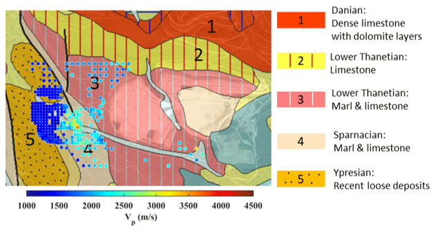
Figure 20 The geological map of the site, obtained from the French Geological Survey (©BRGM; https://www.infoterre.brgm.fr, last access: 11 March 2024), superimposed with the area's satellite view (© Google Earth) and the estimated V_p corresponding to depths of 35–50 m using the W/D method.

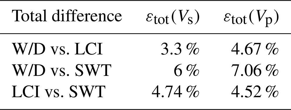
We compute the total differences between the estimated models of every two methods as

$$\begin{array}{}\text{(3)}& {\mathit{\epsilon }}_{\text{tot}}=\left[{\displaystyle \frac{\mathrm{1}}{n\cdot q}}\sum _{j=\mathrm{1}}^q\sum _{i=\mathrm{1}}^n\left|{\displaystyle \frac{\mathrm{1}}{m}}\sum _{k=\mathrm{1}}^m\mathit{\epsilon }(i,j,k)\right|\right]\times \mathrm{100},\end{array}$$

where m, n, and q are the overall number of voxels in z (depth), x, and y directions, respectively. In Table 2, we report the values of the total differences obtained by comparing the models from the three methods. The total difference between the V_s and V_p models obtained from each pair of methods ranges from 3.3 % to 7.06 %. These differences, although not negligible, should not be regarded as substantial, considering the complexity of the near-surface environment. These differences are due to the presence of both significant lateral and vertical heterogeneities and the different parameterization of the methods and interpolation of the models used for comparison. Given that a similar a priori Poisson's ratio was used for LCI and SWT, the total difference between the two methods in terms of V_s and V_p is similar, and the slight difference is attributed to the interpolation and parameterization. In the case of comparing the WD results with those of either LCI or SWT, the difference between V_p models is slightly more (∼ 1 %) than V_s models. The reason is that in the W/D method the V_p models are obtained using the apparent Poisson's ratio. Then, the interval V_p models are estimated through a regularized Dix-type equation. The fact that this process is data transform creates more fluctuating results compared to the layered results of LCI and W/D.

Table 2 The total difference between the estimated V_s and V_p models obtained from the application of the W/D, LCI, and SWT methods.

Table 3 The approximated computational costs for each method.

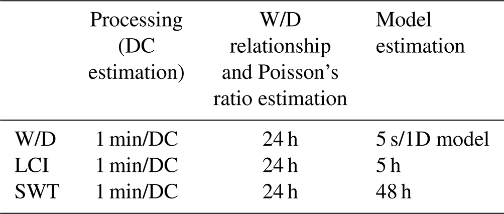
In Table 3, we provide the approximated computational costs for each part of the three methods. The most time-consuming step of all methods is the DC estimation, which also involves expert user intervention. Compared to W/D and LCI, SWT usually requires more DCs to reach adequate data coverage for the tomographic inversion. We estimated 1301 DCs for SWT applied to the north of the site, whereas only 174 DCs were estimated for the application of the W/D and LCI methods to the same zone. The W/D relationship and Poisson's ratio estimation are a common stage for all three methods. The inversion running times (for LCI and SWT) given in Table 3 are for a single inversion trial using 10 CPU cores. Usually, in addition to an unconstrained inversion, several constrained inversions are performed to reach a satisfactory model in schemes of SWT and LCI methods, whereas the W/D method can be applied faster and is efficient for processing large-scale datasets. It is noteworthy to mention that SWT was limited to the northern zone due to computational limitations. The tomographic inversion with 1301 DCs and 300 model points was performed by a workstation equipped with 128 GB of memory and a 10-core CPU. The simultaneous inversion of both zones with at least twice the number of DCs and model points would have required exponentially higher memory and computational capabilities that our workstations could not provide. We could have undersampled the DCs and reduced the number of model points in order to invert both zones together, but we decided to maintain the resolution of the tomographic inversion by focusing on the northern zone only.

In Fig. 20, we show the geological map superimposed with the satellite view of the area and with the horizontal slice of the estimated V_p model from W/D corresponding to depths between 35–50 m. The two diagonal and vertical faults at the north-west of the investigated area separate the east from the west. In the region between the two faults, a gap within the estimated model from the W/D method is observed: the scattering and complex propagation of surface waves that pass through these discontinuities resulted in inconsistencies in the spectrum and prevented the estimation of reliable DCs. The west of the area is characterized by loose formation from recent deposits (outcrop 5 in Fig. 20). The rest of the region is known for stiffer materials, composed of limestone and marl. The estimated V_p also shows a higher velocity in the eastern region. The fastest V_p is registered in the correspondence of the Sparnacian formation (outcrop 4 in Fig. 20). The high-velocity formation from the Danian stage, which is outcropping outside of the investigated area, is probably reached below the depth of 110 m, as all V_s models from the three methods show very high velocity with minor lateral variations below this depth (Figs. 11e, f; 14e, f; and 15e, f).

The application of the calibrated multi-channel (W/D and LCI) and two-station (SWT) methods showed promising results for the processing of the data with irregular source–receiver layout. The W/D method is cost effective and also provides V_p. The other two methods can provide V_p only when an a priori Poisson's ratio is provided. On the downside, W/D is a data transform method, and the noise in the data can directly affect the results. SWT yields high-resolution models when accompanied by extensive data coverage. If the data are restricted to only a few receivers or if there is a limitation on expert resources for two-station DC picking, the performance of the SWT application can be significantly reduced. The use of LCI is highly effective in generating a laterally consistent model from a limited number of DCs. However, in the presence of significant lateral variations, LCI is more prone to excessive smoothing. All three methods depicted a contrast between the limestone-rich area in the east and the loose material in the west, which is corroborated by the geological information. Given the site is an open-cast limestone mining site, the estimated models can offer valuable insights for strategizing the expansion and excavation of the quarry in the investigated zone to support the nearby cement production facility.

7 Conclusions

We showed the application of three surface-wave methods, W/D, LCI, and SWT, to estimate V_s and V_p models using a large-scale test dataset obtained from a hard-rock site through an irregular source–receiver recording technique. The fine-tuned, multi-channel W/D and LCI methods showed potential in the processing of the low signal-to-noise ratio seismic data. Also, the irregular source–receiver outline provided high DC coverage within the two-station method, facilitating high-resolution tomographic inversion. The W/D and LCI methods were applied to both zones outside the mining pits, whereas SWT application was limited to the north of the site. We used the W/D method to estimate a priori Poisson's ratios required for the LCI and SWT methods. The estimated V_s and V_p models from the three methods had differences of less than 6 % and 7.1 %, respectively. The retrieved lateral variation by the methods showed good similarity with the geological information available for the site. The most time-consuming part of the methods is the DC pickings, especially for the SWT method, which requires more DCs to reach adequate data coverage compared to the other two methods. As a result, the automation of DC picking can be viewed as an important milestone in the industrialization of surface-wave methods, facilitating their swift application to datasets even larger than the one used in this study.