Using internal standards in time-resolved X-ray micro-computed tomography to quantify grain-scale developments in solid-state mineral reactions

X-ray computed tomography has established itself as a crucial tool in the analysis of rock materials, providing the ability to visualise intricate 3D microstructures and capture quantitative information about internal phenomena such as structural damage, mineral reactions, and fluid–rock interactions. The efficacy of this tool, however, depends significantly on the precision of image segmentation, a process that has seen varied results across different methodologies, ranging from simple histogram thresholding to more complex machine learning and deep-learning strategies. The irregularity in these segmentation outcomes raises concerns about the reproducibility of the results, a challenge that we aim to address in this work.

In our study, we employ the mass balance of a metamorphic reaction as an internal standard to verify segmentation accuracy and shed light on the advantages of deep-learning approaches, particularly their capacity to efficiently process expansive datasets. Our methodology utilises deep learning to achieve accurate segmentation of time-resolved volumetric images of the gypsum dehydration reaction, a process that traditional segmentation techniques have struggled with due to poor contrast between reactants and products. We utilise a 2D U-net architecture for segmentation and introduce machine-learning-obtained labelled data (specifically, from random forest classification) as an innovative solution to the limitations of training data obtained from imaging. The deep-learning algorithm we developed has demonstrated remarkable resilience, consistently segmenting volume phases across all experiments. Furthermore, our trained neural network exhibits impressively short run times on a standard workstation equipped with a graphic processing unit (GPU). To evaluate the precision of our workflow, we compared the theoretical and measured molar evolution of gypsum to bassanite during dehydration. The errors between the predicted and segmented volumes in all time series experiments fell within the 2 % confidence intervals of the theoretical curves, affirming the accuracy of our methodology. We also compared the results obtained by the proposed method with standard segmentation methods and found a significant improvement in precision and accuracy of segmented volumes. This makes the segmented computed tomography images suited for extracting quantitative data, such as variations in mineral growth rate and pore size during the reaction.

In this work, we introduce a distinctive approach by using an internal standard to validate the accuracy of a segmentation model, demonstrating its potential as a robust and reliable method for image segmentation in this field. This ability to measure the volumetric evolution during a reaction with precision paves the way for advanced modelling and verification of the physical properties of rock materials, particularly those involved in tectono-metamorphic processes. Our work underscores the promise of deep-learning approaches in elevating the quality and reproducibility of research in the geosciences.

1 Introduction

Time-resolved (4D) operando experiments in computed microtomography (μCT) scanners have emerged as a promising way of studying solid-state reactions, offering unprecedented insight into mineral phases and volume changes. This method is becoming a technique of choice for many geoscience problems because it provides information about both the spatial and temporal evolution of the microstructure of a sample. This technique can achieve a range of spatial resolutions, with voxel sizes from millimetres to hundreds of nanometres. Underpinning any usefulness of these new insights is the accurate segmentation of individual phases into three-dimensional (3D) representations across often large datasets; once different phases are segmented and labelled, they directly aid in a quantitative understanding of all types of solid-state mineral reactions (metasomatic, diagenetic, metamorphic, and physico-chemical alteration) (Fusseis et al., 2014).

For the accurate quantification of the various phase components and evolution of minerals from 4D μCT data, semantic segmentation needs to be accomplished. Semantic segmentation refers to labelling individual pixels of an image to a corresponding classification. Image segmentation has long played a pivotal role in the quantitative analysis of digital representations of geological materials, and now there is a wealth of methods available (Reinhardt et al., 2022). However, not all segmentation workflows can effectively track a process in space and time across different samples and acquisition conditions, as is needed in the case of in situ or operando time-resolved X-ray microtomography studies. For instance, while standard histogram segmentation can be consistently applied to a single time step, it may not be easily transferable between different samples undergoing solid-state transformation (Andrew, 2018). More advanced machine learning techniques have been used successfully on a range of geoscience problems and offer better portability and applicability compared to histogram segmentation (e.g. for solid-state reactions (Marti et al., 2021); crack detection (Cartwright-Taylor et al., 2022; Lee et al., 2022; Reinhardt et al., 2022); and one- and two-phase flow experiments (Phillips et al., 2021)), but they also still fall short in achieving complete portability between various time steps. While deep-learning methods show promising potential for tackling the challenges in image segmentation of high-resolution time series datasets, they still need refinement for optimal performance.

Deep-learning algorithms are gaining popularity for analysing microstructures in biological and medical sciences (Renard et al., 2020) and in engineering materials (e.g.  Müller et al., 2021; Allen et al., 2022) and for the segmentation of deforming and reacting porous rock materials (Da Wang et al., 2021). However, regardless of their scientific domains, most studies focus on two-component systems, void, and solid-material classifications. In addition, some deep-learning algorithms still rely on adaptive filtering and global thresholding operations (Phan, 2021). This reliance on the greyscale value can hinder the effectiveness of such algorithms regardless of their complexity. This limitation becomes most apparent in data containing low-contrast phases, where filtering processes to reduce noise or enhance feature visibility may alter or eliminate critical intensity variations necessary for accurate phase differentiation and segmentation. In contrast, convolutional methods, grounded in machine learning, advance beyond these constraints by integrating spatial and morphological information. This integration allows for a more robust and accurate segmentation, especially vital in μCT datasets, where spatial relationships and contextual nuances are key to discerning accurate interpretations. Moreover, in time series datasets, as the greyscale image inputs vary over time, the effectiveness of histogram thresholding diminishes. This is because the optimal threshold for one time step may not be applicable for others, leading to inconsistent or inaccurate segmentations. Greater insight into microstructural changes can only be gained through the full segmentation of all mineral components based on greyscale and other characteristics, like for example component morphology.

This outlines a clear need for deep-learning workflows to be further explored and optimised so that they can be better exploited in geosciences.

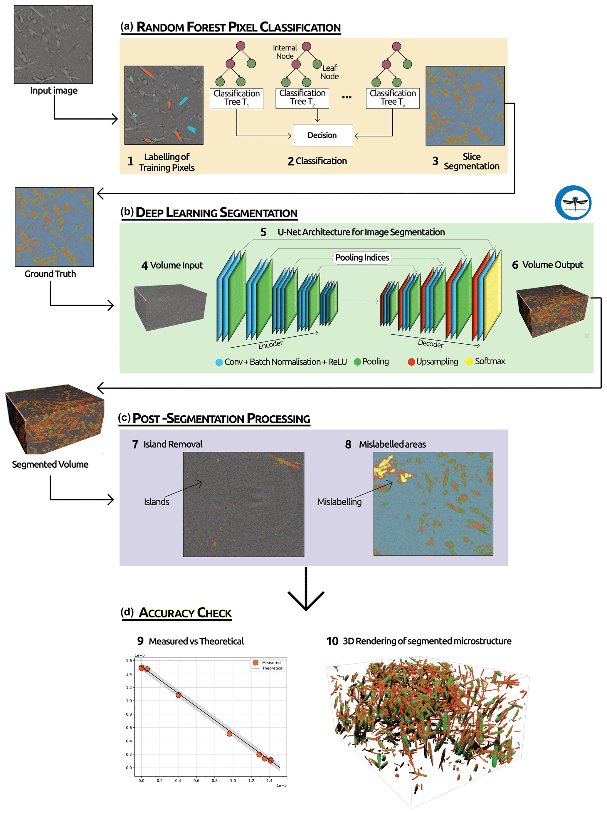
Figure 1 Workflow used for image segmentation. (a) The first step involves manually labelling the different phases (i.e. gypsum, bassanite, pores, celestite) over a few (13) slices in the volume and then applying a random forest (RF) pixel classification. (b) The second step of our segmentation process involves using the output of the RF as ground truth and then running a 2D U-net deep-learning algorithm over the whole selected volume. (c) In the third step we apply a series of post-segmentation routines to clean the dataset of possible segmentation errors. (d) In the final step we quantitatively evaluate the overall performances of the trained deep-learning network by comparing the theoretical and measured molar evolution of gypsum to bassanite during the dehydration.

In this paper, we explore the use of supervised deep learning to segment 4D synchrotron-based computed microtomography (S-μCT) datasets of dehydrating Volterra Alabaster (Fig. 1). Supervised deep learning is a type of machine learning where the model is trained on a labelled dataset. This means that each output produced by the model is paired with the correct output, enabling the model to learn by comparing its predictions to the actual outcomes. This contrasts with unsupervised deep learning, where the model attempts to identify patterns and relationships directly from the input data without labelled outcomes (LeCun et al. , 2015).

For this work we employ a 2D U-Net architecture (Ronneberger et al., 2015) and demonstrate its capability to accurately segment the data into four phases: gypsum, bassanite, celestite, and pores. This model dehydration reaction has been monitored during experiments under different stress and pore fluid pressure conditions (Gilgannon et al., 2023). The data used encompass numerous challenges encountered in volumetric image segmentation of complex materials, including multiple heterogeneous material phases with feature sizes ranging from hundreds of nanometres to micrometres, low contrast between phases, and a relatively rapid evolution. We demonstrate that these factors make segmentation using standard approaches difficult. We quantitatively compare outputs of the deep-learning architecture to optimise its use and for the first time show how the accuracy of segmentations can be checked with an internal standard given by the chemistry of the system. Ultimately, we find that the use of a random forest classifier to produce the “ground truth” to the training of the deep-learning architecture improves the predictive abilities of the algorithm. While the random forest algorithm initially can effectively segment features of interest in our dataset, its capability for generalisation to new, unseen data is limited (Rezaee et al., 2018). The inclusion of the deep-learning step enhances the generalisation capability of our workflow. This provides significantly improved accuracy and validity of the segmentation and labelling of the S-μCT data during the solid-state reaction of gypsum to bassanite and pore space. We believe that this work demonstrates the potential of deep learning for volumetric image segmentation of complex materials. The method is generic and can be applied to other geoscience problems.

2 Gypsum dehydration as an example of a complex segmentation problem

2.1 The gypsum dehydration system and experimental set-up

Gypsum dehydration is used as a model dehydration for many prograde metamorphic reactions in collisional tectonic settings. The physical boundary conditions make it amenable for laboratory studies and thus a system of choice to investigate complex geological problems in time-resolved μCT in situ experiments.

Volterra alabaster is a rock that is mainly (> 90 %) composed of gypsum (CaSO₄⋅2H₂O) and celestite (SrSO₄), and when the temperature is increased the gypsum dehydrates to produce bassanite (${\mathrm{CaSO}}_{\mathrm{4}}\cdot \frac{\mathrm{1}}{\mathrm{2}}{\mathrm{H}}_{\mathrm{2}}\mathrm{O}$), porosity, and water. At the same time, celestite remains stable during gypsum breakdown and is unaffected by the dehydration. The dehydration of gypsum results in a 29 % reduction in solid molar volume and an 8 % excess volume of water. Experiments were performed with the X-ray transparent triaxial rig Mjölnir (Butler et al., 2020) at the TOMCAT beamline of the Swiss Light Source (SLS) synchrotron. All of our experiments were performed at the same confining pressure (P_c) of 20 MPa and a pore fluid pressure (P_f) varying between 1 and 5 MPa. The experiments followed the same temperature path, with a maximum temperature of 124.5 < T < 126.9 °C. We systematically varied the differential stress in each experiment to capture its effect (σ_diff = 0; 16.1; 27.9 MPa; see Gilgannon et al., 2023). For the work presented in this paper, we focus on data from two specific experiments, chosen as “end-member” scenarios for their distinct evolving mineral fabric during the dehydration process: (i) a sample, VA17, where the principal stress is radial (with σ_diff = 11.3 MPa), and (ii) another sample, VA19, where the principal stress is vertical (with σ_diff = 16.1 MPa). Time-resolved (4D) synchrotron computed microtomography datasets were acquired during the experiments at SLS TOMCAT beamline using a filtered white beam with an energy peak at 27 KeV. For each S-μCT dataset, 1500 radiographs were collected over 180° rotation in 2–4 s. The resulting radiographs had a voxel size of 2.753 µm, and the resulting 3D μCT datasets had a size of 2016 voxel × 2016 voxel × 2016 voxel. The frequency rate of the tomoscopy was set to 60 s, and the experiments ran over 150–314 min, resulting in 2.5 TB of data to be analysed. More details on the experiments can be found in Gilgannon et al. (2023).

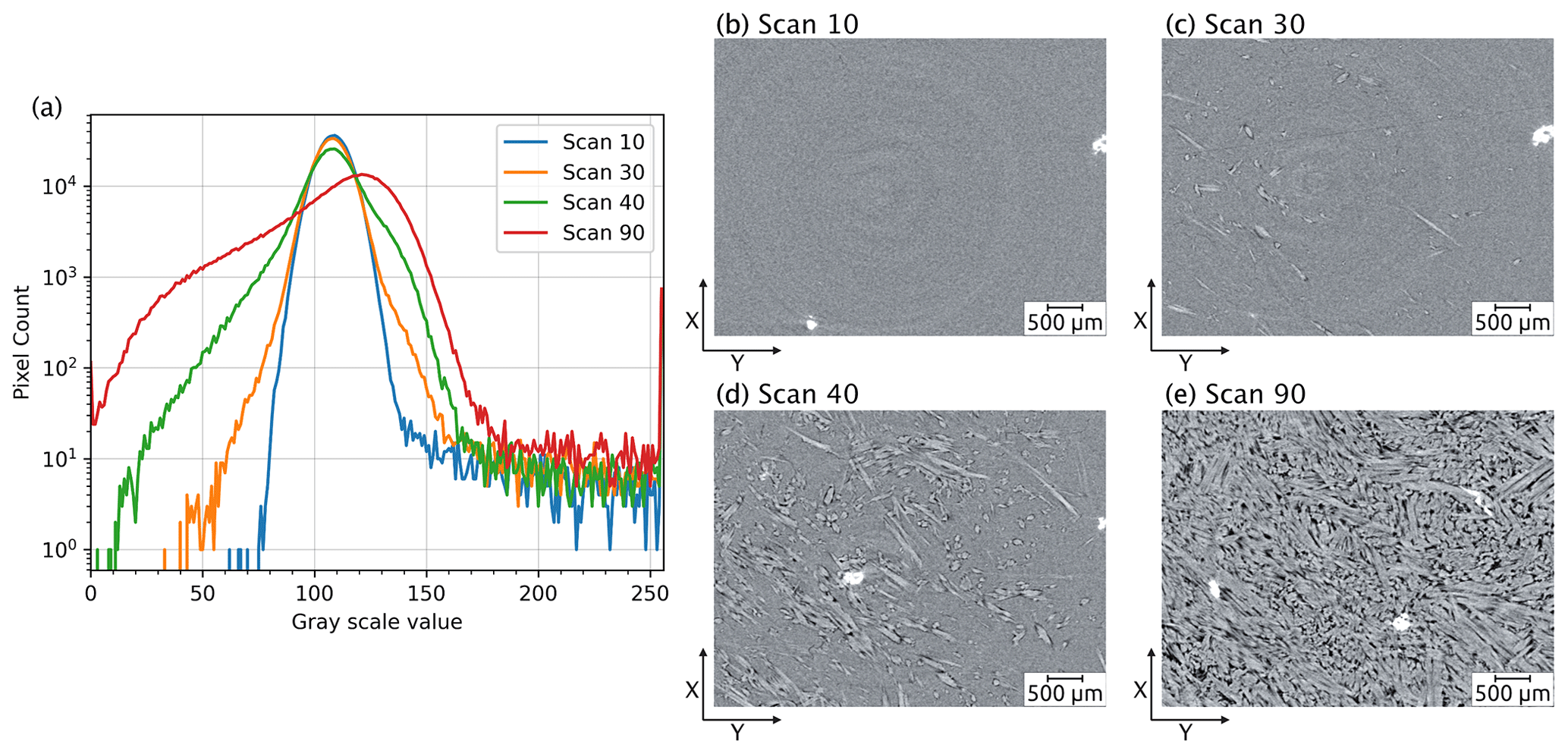
Figure 2 Variation in greyscale intensity values with reaction progress. (a) Greyscale histograms of a series of tomographic slices captured at different stages during the reaction. Each line represents the histogram of an individual slice in the tomographic scan, illustrating the changes in greyscale intensity value distribution across the time steps. This variation complicates the use of greyscale thresholding as input for the deep-learning model. Panels (b–e) display the slices corresponding to the histograms in (a), depicting the reaction progression from an early stage (b) to the final product (e).

2.2 Challenges of segmenting dehydrating gypsum during operando X-ray microtomographies

It is clear from Fig. 2 that microstructural changes during the experiment can be readily identified by the human eye. However, it is also apparent from the evolving histograms in Fig. 2a that accurate segmentation of the four phases of interest (i.e. gypsum, bassanite, pores, and celestite) cannot rely on simple histogram thresholding segmentation, as the optimal threshold varies across different time steps. Each 4D S-μCT dataset is extensive, containing more than 100 scans, each ranging from ∼ 5 to ∼ 15 GB of reconstructed data, depending on the scanning parameters. As the histograms of individual scans are clearly different for different time steps (Fig. 2a), an automated segmentation of the evolving volumes based on a single histogram would yield inaccurate results, necessitating manual segmentation and the explicit selection of thresholds for each tomogram and for each experiment. This laborious process inhibits the efficient analysis of large 4D datasets but also misses basic standards for reproducibility. This is further complicated by the fact that all S-μCT images have a symmetrical vertical gradient in noise through the sample, first decaying and then increasing, which renders the application of a single set of thresholds even to a single S-μCT dataset problematic. Additionally, the homogeneity of the unreacted starting material intensifies artefacts such as rings, which are problematic to handle for segmentation algorithms that are based solely on greyscale thresholds. As noted above, the human eye can distinguish different phases in the data, and this suggests that a learning-based approach to semantic segmentation would be applicable to the dataset. It is becoming evident that we may also require information beyond greyscale values, such as the geometry of the feature of interest, for successful segmentation.

2.3 A segmentation workflow with internal standards

To accurately segment large datasets of dehydrating gypsum samples, we used deep-learning algorithms, which have entered the field of volumetric image segmentation through the implementation of convolutional neural networks (CNNs). For this work, we used a specific implementation of 2D U-Net available in the Dragonfly™ software. This implementation has performed well on μCT images from fibre-reinforced ceramic composites (Badran et al., 2020). Our dehydrating gypsum datasets are comparable in terms of greyscale value contrast and the number of distinguishable material phases. Dragonfly runs locally on a workstation and allows for the creation of training data and training of a CNN segmentation model. Once the CNN is trained, the model can be generalised and offers the advantage of being flexible and straightforward to apply on similar datasets.

To train the network, we selected 13 of the 2016 horizontal (XY) virtual slices from the synchrotron CT scan of sample VA19 time step 40 as “input” images. This specific time-step was chosen because it has sufficient volume of each phase we aim to segment; in images derived from either early or late steps of the experiment, the volume of at least one of the phases would be insufficient to achieve automatic segmentation. We tested the role of ground truth data (i.e. the correct segmentation of an image) in achieving the best results by comparing a histogram thresholding segmentation with a random forest classifier.

Choosing the best training neural network architecture and tuning the network (hyper-)parameters – i.e. those settings of the model that are set prior to training and remain constant during the training process – requires time and some knowledge of neural network architecture. However, once the best configuration is set up, the application of the model is nearly effortless. Network (hyper-)parameters that need to be chosen include (i) a “patch size”, in the training stage the images are split into a set of smaller 2D square patches that capture the features of interest in the image; (ii) a “stride ratio”, which defines the position of the neighbouring patches (at a value of 1.0, there will be no overlap between patches, and they will be extracted sequentially one after another; at a value of 0.5, there will be a 50 % overlap); (iii) a “batch size”, which defines the number of patches evaluated in each batch prior to updating the network model; (iv) the number of epochs, an epoch indicates a training iteration, involving a pass over all batches of the training set; and (v) a selection of a loss function to evaluate how far the output of the CNN model deviates from the ground truth and an optimisation algorithm to find optimal weights for the coefficients of the CNN.

We trained the different networks by varying the (hyper-)parameter settings to see which setting results in a measurable improvement to model performance. For all the tested strategies, we randomly choose 20 % of the segmented data to serve as a “validation set” that is otherwise not used during training. A loss function was used to evaluate the training progress. The U-Net deep-learning architecture was trained for a maximum of 100 epochs, stopping when no further improvement of loss was observed.

To demonstrate the accuracy of the segmentations, we devised an additional quality check consisting of comparing the output volumes of phases to their predicted values given by the mass balance of the reaction (see Sect. 3.7). This internal standard allows us to objectively assess the effectiveness of the application of deep learning to time series datasets that contain low-contrast phases.

3 Influence of training data

3.1 Input data for the deep-learning convolutional neural network

Convolutional neural networks (CNNs) are a special class of deep-learning algorithms where one or more layers of the network perform convolution operations (Fig. 1). The specific convolution kernels are not programmed but are learned from the input data by the deep-learning engine to extract relevant features of an image that become useful discriminators in segmenting complex pixel classes – in our case mineral phases – in the images. The CNN architecture (Fig. 1b) can be thought of as a formula of linear weights applied to the image pixel intensities, often combined through multiple network layers in a nonlinear fashion. The coefficients encoded in the neural network itself are learned from training data that couples example “input” images (i.e. the raw un-segmented image) with example “output” images (i.e. ground truth). The iterative process of learning the weights that can reliably transform input into output images is termed “training” and is the most computationally demanding phase of the deep-learning cycle. In order for a deep-learning model to perform the segmentation of the different classes contained within the image, it requires a set of data that are typically created by manually annotating each pixel in the image with its corresponding semantic label (Fig. 1a). This set of labelled pixels forms the so-called “ground truth”. Ground truth is an essential part of training deep-learning models as it represents the target to learn towards and should ensure that the model is learning to segment images in a meaningful way. In our case, the ground truth images are a selection of image slices that have been previously segmented to assign each pixel to a specific mineral or pore phase. The trained model can then automatically segment not only the remaining unsegmented image slices within a single μCT volume but also unseen data – i.e. other volumes within the same time series of the training set and image volumes obtained during other experimental time series.

To establish the ground truth set for initial image classification, we initially considered methods with differing informational depths. One such method is histogram thresholding, which relies on basic greyscale values and typically results in low-information-level outcomes. However, this approach alone proved inadequate for our purpose, as it often led to gradients with diffuse phase boundaries, underscoring the need for more sophisticated classification methods. In contrast, ground truth classified using a machine learning algorithm provides discrete transitions between phases and better information about features like phase morphology. Before finding the best workflow to segment our image volumes, we tested several combinations of ground truth input and CNN parameters until the quality of output images on unseen data was adequate, with reasonable training time (Fig. C1 and text in Appendix C).

Figure 3 Challenges of the segmentation. (a) Portion of a cross-sectional slice of the raw μCT image showing the relative low contrast between gypsum and bassanite. (b) Threshold values for the four phases present in the image. Two main phases – gypsum and bassanite – are difficult to split up accurately into two classes by the deep-learning algorithm with (c) no data augmentation but are better segmented when using data augmentation (d) but still showing evident artefacts in the segmentation. Both cases (in c and d) struggle at separating the celestite phase, which is wrongly classified as bassanite. (e) The segmentation results using a random forest classifier as input into the deep-learning algorithm.

3.2 Histogram thresholding as training data

Figure 3a shows an example of data containing the four phases as segmented by different networks trained with different ground truth data. The corresponding colour-coded threshold values for the four phases are shown in Fig. 3b. Figure 3c shows the output produced by a neural network trained using a ground truth set of images labelled solely by manual histogram thresholding. This input failed to reliably classify the bassanite needles, it often failed to segment pores, and it failed to accurately segment celestite, often confusing it for bassanite. This can be improved upon by using manual histogram thresholding with the application of data augmentations within the neural network model (Fig. 3d). The training data were subjected to data augmentation based on the basic image manipulations (i.e. flip horizontally, flip vertically, rotate, shear, and scale). Specifically, we octupled the input data (i.e. generating eight variations of each original image) in order to increase its initial size, rendering the neural network more robust, while at the same time compensating for deliberately using a small input dataset. This strategy allowed us to increase the network's ability to generalise while decreasing the potential danger of overfitting (Shorten and Khoshgoftaar, 2019). By tuning the different CNN (hyper-)parameters and including augmented data, we improved the overall performance of the network (Fig. 3d). However, the final segmentation still lacked accuracy: it can be seen that errors remained, for example the celestite was still identified as bassanite (Fig. 3d). More importantly, this deep neural network model struggled when it was applied to new and more complex datasets: such as in the early and final stages of the reaction (where one of the two main phases was scarce or absent).

3.3 Random forest classifier as training data

In contrast, the use of ground truth data classified with a random forest classifier plus data augmentation performed exceptionally well and visually captured more of the features of the microstructure correctly (Fig. 3e).

A random forest classifier (Fig. 1) comprises numerous decision trees, each contributing a vote toward the class prediction for every voxel (more details on the random forest classifier are available in the Appendix). The class receiving the most votes is allocated to the respective voxel. Filters are applied to the input images, generating filtered images that serve as features (Reinhardt et al., 2022). These features enable the classifier to differentiate between phases in the dataset. In this work, the random forest classifier was pre-set with morphological filters, a 3 × 3 neighbour filter, and a Gaussian filter to perform identification of the phases in the training set. Using a random forest classifier for setting up the ground truth dataset also enabled training the deep-learning model based on the shape of the objects. This offered a significant progress from manual thresholding segmentation.

Table 1 Evaluation of the segmentation models based on Dice coefficient scores.

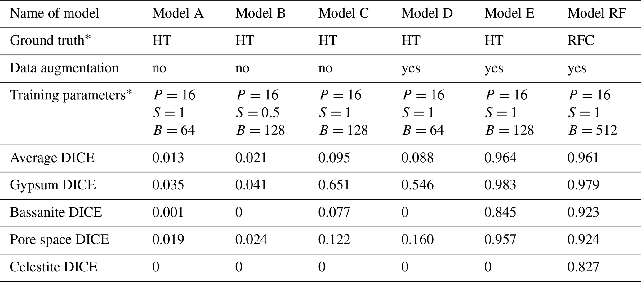
^∗ Abbreviations are as follows: HT is histogram thresholding, RFC is random forest classifier, P is patch size, S is stride ratio, and B is batch size

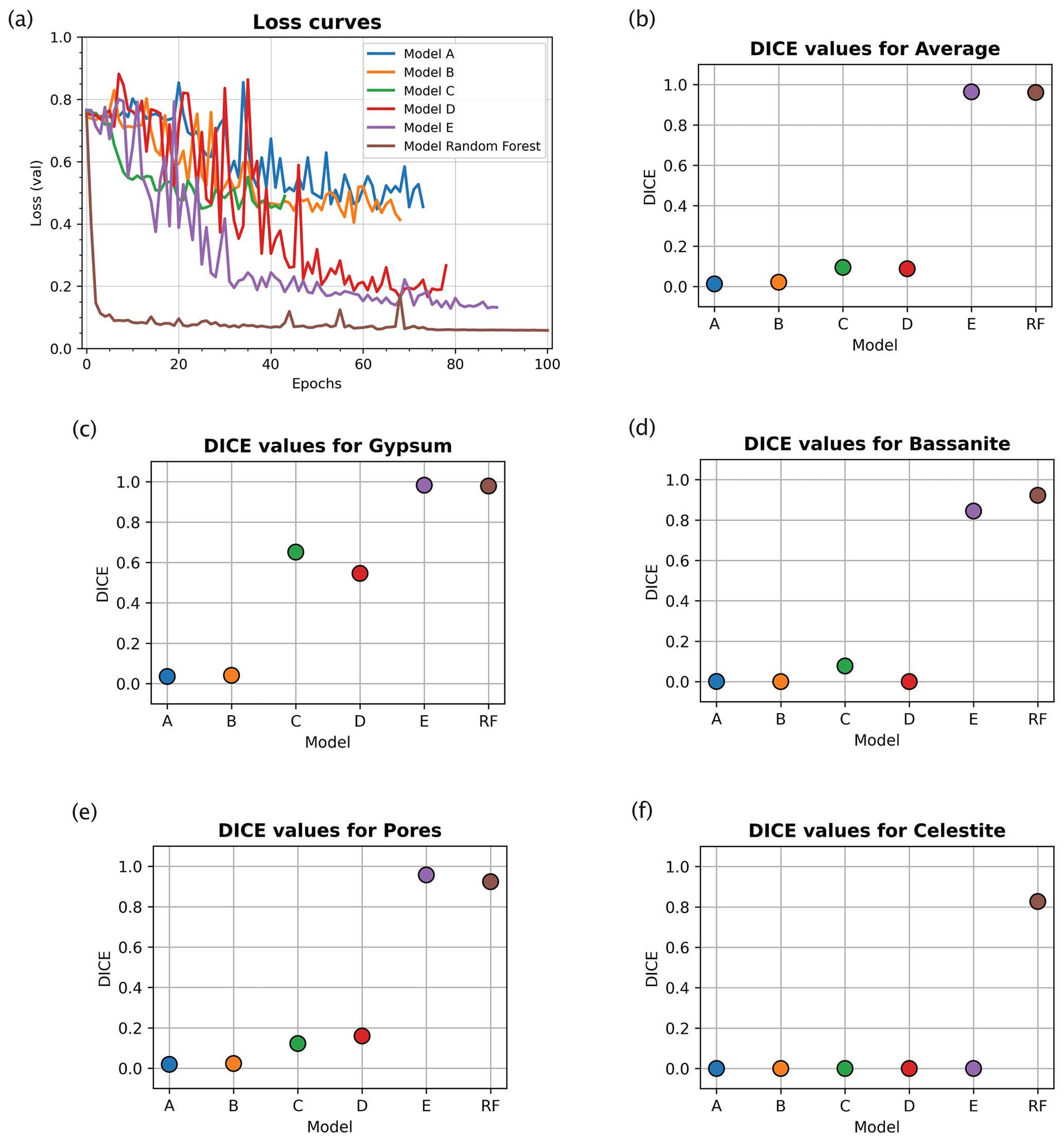
Figure 4 Error curves and evaluation metrics for the image segmentation models (see Table 1 for details of the models). (a) Error curves comparison for different loss values for the tested models. The neural network model trained with a random forest classifier input outperformed the other models that used manually thresholded inputs. Plots for Dice coefficient (DICE) metric (colour coded as in a) show the predictive performances of each trained model for both the average volume (in b) and each separate phase: gypsum (c), bassanite (d), pores (e), and celestite (f). Clearly, the model trained using a random forest classifier input demonstrates superior performance to other models. See Table 1 for details of the training parameters for the different models.

3.4 Optimising the deep-learning models

Model parameters can be optimised to improve the deep-learning network. We systematically monitored the performance of each tested deep-learning model during both training and testing. The results of this systematic testing are visualised in Fig. 4 and synthesised in Table 1. The quantitative comparison of types of ground truth data and the variations of model (hyper-)parameters provides a solid base for discussing the advantages of the workflow that is presented here and how it is transferable to other geoscience data.

For an objective quantitative comparison of different deep-learning network models, we tracked the performance of each model during training using a loss function to measure the error between the neural network's prediction and the corresponding ground truth; the error was then used to update the model parameters. Figure 4a shows that with ground truth data derived from random forest classification we obtained the lowest validation errors for all tested networks. Compared to other models, the random forest model reached low values of loss already after five epochs. After this minimum, the error kept oscillating within the neighbourhood of its lowest value until the maximum 100 epochs were reached. This indicates that the overfitting risk is minimal.

We evaluate segmentation quality according to eight standard evaluation metrics based on overlap and similarity criteria (Taha and Hanbury, 2015; Müller et al., 2021), where the deep-learning-based segmentations are compared to the corresponding ground truths. Here we focus on the Dice coefficient, however, a full picture of all calculated metrics can be found in the Supplement. The Dice coefficient scores were used to evaluate and compare the segmentations resulting from neural network models trained on (i) histogram thresholding ground truth data (models A, B, and C), (ii) histogram thresholding with augmented ground truth data (models D and E), and (iii) random forest classified ground truth data with augmentation (model RF). The Dice coefficient (DICE) is the normalised overlap of pixels in the segmentation and the corresponding ground truth of a given phase. A DICE score of 0 means that there is no overlap between segmentation and ground truth, while a DICE score of 1 indicates perfect overlap. In addition to the direct comparison between automatic and ground truth segmentations, it is common to use the DICE to measure reproducibility (repeatability) of a trained neural network segmentation algorithm (Taha and Hanbury, 2015).

For the networks trained using histogram thresholding, the average DICE varies between 0.01 and 0.98, and it increases when data augmentation is used during training. For the network trained using a random forest classifier, the DICE score is also 0.98 (Table 1). From the error curves and the DICE plots, it is clear that the inclusion of augmented data into the histogram threshold ground truth (as seen in models D and E in Fig. 4 and Table 1) improved the overall performance of the neural network model compared to the models which did not (models A, B and C in Fig. 4). The DICE scores for each segmented phase show similar trends, on average improving for data augmented models. However, it was only the model trained using a ground truth from a random forest classifier that produced scores for all four phases. This includes the celestite phase, which was entirely absent in the results from the other models (Fig. 4).

All of these results show that when using random forest classifier, pre-classified ground truth data clearly outperform a ground truth obtained via simple greyscale histogram thresholding regardless of the optimisation of parameters.

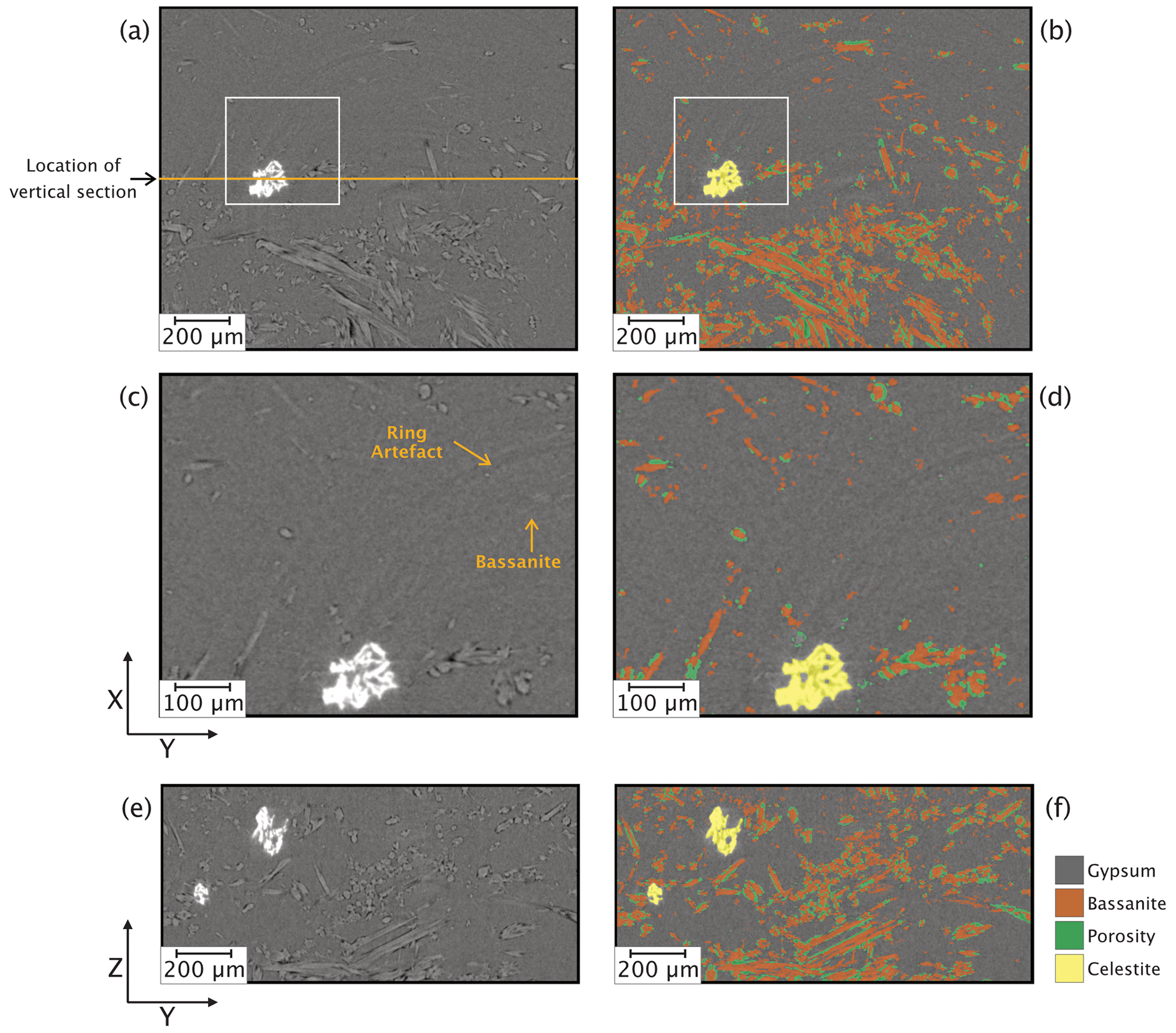
Figure 5 Horizontal (XY) and vertical (YZ) slices of the S-μCT images before (a, c, and e) and after (b, d, and f) deep-learning segmentation performed using a model trained with random forest classified images. Images in (c) and (d) are magnified views of areas indicated with white boxes in (a) and (b).

3.5 Applying the deep-learning segmentation

After the training stage, the model was applied to a larger sub-volume (400 consecutive slices, ∼ 250 MB) from the same scan used during training of the deep-learning algorithm (i.e. VA19 time step 40). The model succeeded in correctly segmenting all four phases in about 7 min using a computer with 256 GB of RAM, an Intel Xeon 18-core processor, and a 16 GB NVIDIA Quadro RTX 5000 graphics processing unit (GPU). Typical results are shown in Fig. 5, which compares equivalent horizontal and vertical slices from the unprocessed and segmented CT images. This comparison indicates that gypsum, bassanite, porosity, and celestite are clearly labelled, even in the portions showing ring artefacts that can mask the true greyscale values (Fig. 5c and d). Importantly, the combination of random-forest-based ground truth and deep-learning segmentation ensures that the ring artefacts are not mislabelled as actual phases, a problem that frequently arises with manual histogram thresholding. This consequently prevents the creation of fictitious phases when there are none. Comparison of the vertical (YZ) sections (Fig. 5e and f), where the unprocessed slice clearly shows all four phases, qualitatively indicates that the accuracy of the segmentation is high.

3.6 Post-segmentation processing

Once the data volume is segmented by the trained deep-learning model, we apply a series of post-segmentation routines to clean the dataset from segmentation errors, which is necessary primarily on data acquired early in the experiment when the contrast in the sample was low. These routines involve removal of isolated clusters of erroneously labelled pixels and deletion of areas labelled as bassanite around celestite aggregates. The first routine is implemented using the “remove island” tool in Dragonfly™, targeting pixels misinterpreted as bassanite and porosity. The size of clusters to be removed is fixed in all volumes of the time series and also through the different scanned samples: 100 and 8 pixels for bassanite and porosity, respectively. The application of this routine is much more frequent at early stages of the dehydration process when the majority of the volume is still represented by the gypsum phase: the lack of contrast between phases leads to very noisy slices (i.e. speckled in appearance). The second routine involves the deletion of mislabelled areas around celestite. This procedure is most accurate and fast if conducted through visual inspection and manual corrections.

3.7 Understanding the accuracy of the segmentation

Time-resolved μCT data offer the opportunity to quantify evolving volumes in a sample and thereby the rates of a process, whereby the accuracy of the quantification hinges on the accuracy of the volumetric segmentation. The accuracy of our deep-learning segmentation method itself is contingent upon three potential sources of error. The first pertains to the quality of the original CT image data, influenced by factors such as image resolution, noise, and potential artefacts. In our work, this source of error had minor impacts on the segmentation of bassanite and pores and is primarily restricted to the early stages of the dehydration process when the dominant presence of a single mineral phase, gypsum, led to noisy slices and enhanced ring artefacts. A second potential error source lies in the initial segmentation used to establish the target image. The initial segmentation is arguably the most laborious and time-consuming step, with some level of error inevitable during the labelling of slices and assignment of pixels to specific phases, particularly at phase boundaries. These issues, however, have minimal impact on the final trained model as they generally occur at isolated pixels (Badran et al., 2020). The third potential source of error is mislabelling of pixels during the deep-learning segmentation stage, attributable to limitations in the accuracy of the trained model. While the error rate typically decreases with an increase in the number of training images and iterations, overfeeding the training network can lead to overfitting, which can in turn degrade performance when segmenting unseen images. However, we showed (Figs. 3 and 4; Table 1) that augmenting data significantly reduced both mislabelling and overfitting during the training step of the neural network.

The quantification of a metamorphic reaction rate from 4D μCT data hinges on the accurate tracking of the evolution of reacting and emerging phases. To independently ascertain the accuracy of the chosen deep-learning model, we compared the theoretical and measured (i.e. segmented) molar volumetric evolution of gypsum to bassanite during the dehydration reaction.

For the case studied here, where no irreversible compaction occurred in the samples during the experiments (Gilgannon et al., 2023), we can use the theoretical molar evolution during the dehydration of gypsum to bassanite to calculate the amounts of gypsum, bassanite, and water produced during the dehydration reaction and the stoichiometric ratios between them. Gypsum has two water molecules per formula unit, while bassanite has only half of a water molecule per formula unit. Hence, during the dehydration process, the molar ratio of water molecules to calcium sulfate molecules decreases. The chemical equation for the dehydration of gypsum to bassanite is as follows:

$$\begin{array}{}\text{(R1)}& {\mathrm{CaSO}}_{\mathrm{4}}\cdot \mathrm{2}{\mathrm{H}}_{\mathrm{2}}\mathrm{O}\to {\mathrm{CaSO}}_{\mathrm{4}}\cdot \mathrm{0.5}{\mathrm{H}}_{\mathrm{2}}\mathrm{O}+\mathrm{1.5}{\mathrm{H}}_{\mathrm{2}}\mathrm{O},\end{array}$$

where one mole of gypsum (CaSO₄ ⋅ 2H₂O) gives one mole of bassanite (CaSO₄ ⋅ 0.5H₂O) and 1.5 water molecules.

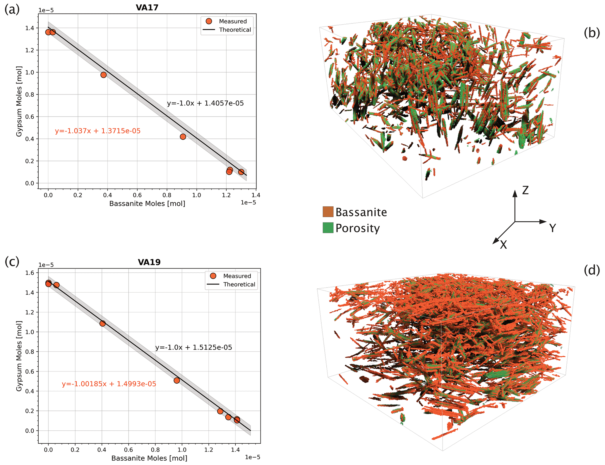
Figure 6 Theoretical versus measured values. Comparison between the theoretical and the measured molar ratio of gypsum and bassanite during dehydration. Here, we plot the evolving molar ratio of gypsum to bassanite during dehydration for (a) sample VA17, which experienced radial stress and (c) sample VA19 experiencing axial stress (see Fig. 5 for reference). Shaded grey areas are 2 % confidence intervals of the theoretical curve. On the right-hand side, 3D renderings of bassanite crystals and pores in two samples' sub-volumes reacting at two different stress conditions. In (b) the VA17 reaction principal stress (σ_max) is axial (i.e. parallel to Z), while in (d) VA19 the principal applied stress is radial (in the x–y plane). The height of both boxes is 1.5 mm.

Knowing the initial volume of gypsum in the sample and its density (2310 kg m⁻³), we can simply calculate its mass and the corresponding molar quantity. From this, we can compute the theoretical amount of bassanite produced from gypsum at every reaction step. Given that the density of bassanite is 2731 kg m⁻³, we can use the molar mass to convert the produced moles of bassanite into volume. A plot of the moles of reactants versus products is a $y=-x$ graph consistent with the 1:1 stoichiometric ratio of reaction (Eq. 1). For the 1:1 gypsum-to-bassanite reaction, the slope is −1 (solid black lines in Fig. 6a and b with grey-shaded 2 % confidence intervals). The segmentation, which provides a volume of bassanite and gypsum at each step, can be represented and compared to the theoretical case. This graphical method forms the basis of the theoretical dehydration curve against which we compare the segmented volumes. Examples of this comparison are shown in Fig. 6, where we present dehydration evolution paths for a sample under radial stress (VA17, Fig. 6a) and an axial deviatoric stress sample (VA19, Fig. 6c). In both examples, the curves for theoretical and measured molar volumes follow the same trend, with fitting parameters showing close equivalence.

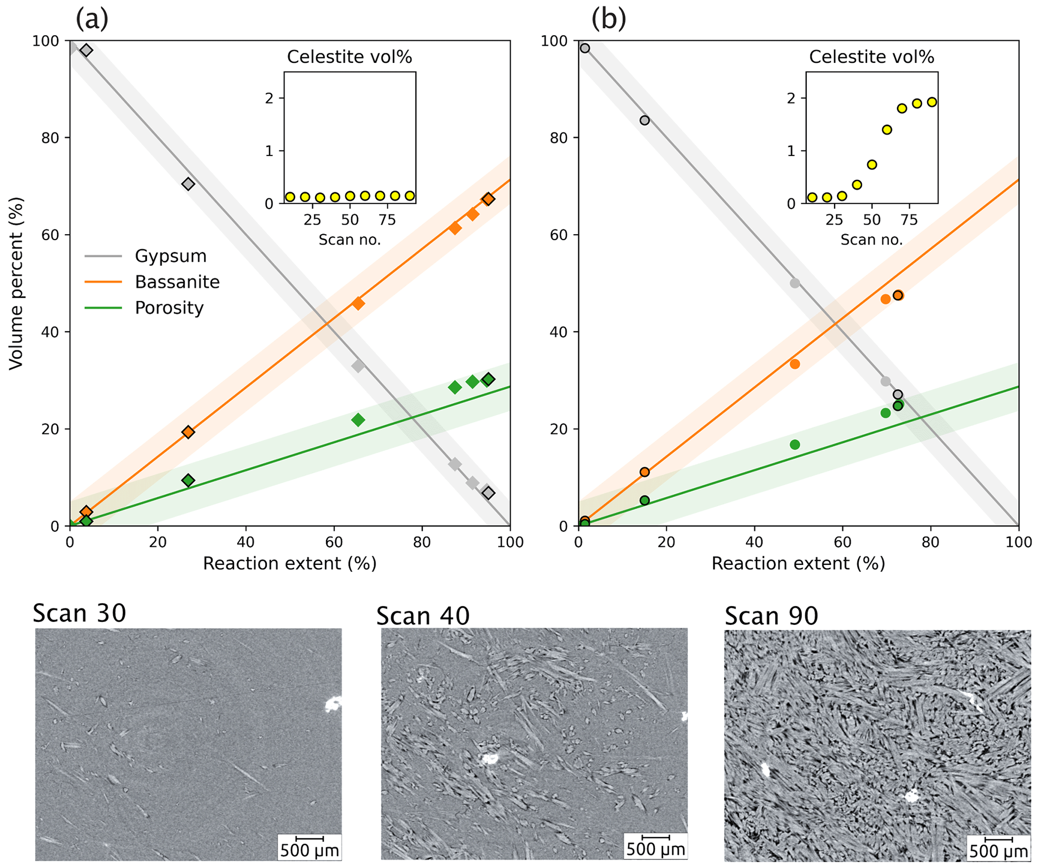
Figure 7 Quantitative analysis of phase volume changes during the gypsum dehydration experiment, as determined by segmenting the same time series data (sample VA19) using two distinct segmentation methods. The new workflow developed in this study in (a), which leverages a random forest classifier to label input data for a deep-learning model, yields significantly improved accuracy in phase volume measurements relative to conventional histogram thresholding segmentation in (b) – including “despeckle” and “non-local means” with sigma = 5 and smoothing = 1. The inset graphs show volume measurements for the celestite phase (yellow), which is a non-reacting phase during dehydration. The bottom images show slices of the sample at different stages; in the graph they are represented by the data points with a black outline.

This comparison shows that our segmentation workflow produces highly accurate volume fractions for each phase. All fractions fall within the < 5 % error bound of the theoretical curve (Fig. 6). For a more comprehensive evaluation of the method, a comparison was made between the novel integrated workflow (Fig. 7a) and traditional manual histogram thresholding. This comparison was applied to a selection of volumes in the time series (Fig. 7b). The manual thresholding method, which incorporates basic pre-processing steps (including “despeckle” and “non-local means” with sigma = 5 and smoothing = 1) displayed significant shortcomings. It resulted in a severe underestimation of the reaction extent and the inadvertent “creation” of celestite. Contrarily, the proposed workflow (Fig. 7a) significantly outperforms the traditional approach (Fig. 7b).

Due to its demonstrable accuracy, the segmentation output is well suited for extracting quantitative information, such as mineral growth rates and variations in pore size during the dehydration reactions. Our segmentation method enables the quantification of relative accuracy, allowing for the propagation of errors in any derived and quantified parameters. This advance represents a significant step towards interpreting results and establishing their significance, as confidence intervals are often absent in studies using manual thresholding.

4 Discussion and implications

The application of deep learning to time-resolved micro-CT imaging offers a new tool for geoscientists studying rock deformation, metamorphic processes, and fluid–rock interactions. We successfully leveraged optimised deep-learning methods to perform reliable and efficient segmentation of time-resolved volumetric images during the gypsum dehydration reaction. The approach outlined here not only streamlines data analysis by swiftly processing large datasets but also enhances confidence in the robustness of results by ensuring high segmentation accuracy. To ascertain the accuracy of the chosen deep-learning model we compared the theoretical and measured molar evolution of gypsum to bassanite during dehydration. This approach defines an internal standard, verifying that the segmentation method accurately captures the mineralogical changes occurring within the rock samples. Importantly, the robustness of this validation is based on the three-component nature of the system – gypsum, bassanite, and water (imaged as porosity the S-μCT data) – allowing for a non-circular and independent verification of our method's effectiveness. By harnessing the power of deep learning for image segmentation, we can extract more nuanced and precise information from μCT imaging datasets. This will enhance our understanding of geological processes and contribute to more accurate models of rock behaviour under different physical conditions.

4.1 Comparison with other segmentation approaches

Accurate segmentation has long been a challenge across various scientific domains, from medical CT imaging to material sciences and engineering (Withers et al., 2021). Global segmentation methods, such as manual histogram or watershed thresholding, have long been go-to solutions for the segmentation of X-ray CT tomographic images. However, the following three considerable drawbacks persist: (i) the significant time commitment required, (ii) the fact that global techniques ignore local context and thus have an intrinsic potential for misclassification, and finally (iii) the potential for compromised reproducibility (Andrew, 2018). As CT imaging technologies evolve, resulting in larger datasets, the scalability and efficiency of manual segmentation methods become increasingly challenging (Da Wang et al., 2021). Herein lies the risk of jeopardising reproducibility, defined as the ability to consistently obtain similar results across multiple measurements using the same methodology (Renard et al., 2020).

Machine and deep-learning segmentation strategies form promising alternatives for automatic segmentation, optimising parameters for high accuracy performance on the training dataset and ensuring effective generalisation to other datasets within the same problem class. However, transitioning towards automatic segmentation, while promising, is not trivial. Successful automation of segmentation methods still requires an initial investment of time and resources for skill acquisition and understanding needed to fine-tune models and adapt the workflow to the specific dataset at hand.

A good example of this is the intrinsic dependency of deep-learning segmentation on the ground truth data input and the selection of (hyper-)parameters during the training process. If the initial segmentation – which forms the ground truth – is not meticulously executed, this could lead to sub-par results. These could manifest as minor differences when compared with the ground truth, creating a misleading perception of accurate segmentation. Given these potential pitfalls, independent verification of segmentation results appears to be a preferable approach.

In fields such as medical imaging and material science a common strategy to ensure reliability and accuracy of segmentations is the use of external calibration techniques, which involve the use of phantoms with known dimensions and/or compositions as benchmarks (Adams, 2009; Kruth et al., 2011). These external standards aid in the assurance of measurement accuracy (Withers et al., 2021). However, these calibration techniques are not without limitations. One major challenge lies in partial volume effects, which occur when the volume of interest encompasses more than one type of material. The CT values measured in these regions do not correspond to a single material type but rather are a weighted average of the different types present (Kruth et al., 2011; Sokac et al., 2020). Solutions have been proposed and often require complementary techniques (such as using tactile, optical sensors) to calibrate measurements derived from CT data (Torralba et al., 2018). Reinterpreting segmented voxels using greyscale values can offer a complementary method for calibration. This approach assigns partial values to affected voxels, potentially enhancing accuracy in cases of overlapping mineral phases or partial volume effects. Furthermore, the use of phantoms can result in difficulties during sample preparation (such as staining, sample chemistry or structure modification to include the standard) which can in turn alter the general output of the segmentation.

In line with the efforts to enhance the accuracy and reproducibility of CT image-based measurements, our approach leverages a priori knowledge of the chemical reactions involved in the dehydration process, therefore establishing a framework for assessing the accuracy of the data extracted from the CT images. This internal validation approach offers a robust and consistent means of assessing the reliability of our segmentation results. It provides an additional layer of confidence in the accuracy of our measurements, ensuring that the segmentation method effectively captures the phase evolution within the rock samples.

4.2 General applicability of the proposed workflow

The versatility of the presented workflow extends beyond the study of the gypsum dehydration process. By leveraging 4D CT imaging and integrating chemical knowledge, our approach has potential for investigating other fluid–rock interaction processes, enabling precise quantification of mineralogical changes, and providing valuable insights into various geological phenomena. For example, our approach can be directly applied to the investigation of the KBr−KCl solid–solid replacement, which serves as an analogue for studying the dolomitisation mechanism and other solvent-mediated reactions, resulting in the creation of porosity (Beaudoin et al., 2018). Similarly, the method has potential in fluid–rock interaction reactions relevant in the geoenergy field: our methodology can contribute to the analysis of carbonation reactions within ultramafic rocks, where carbon dioxide (CO₂) reacts with minerals to form carbonate minerals (Beinlich et al., 2020; Snaebjörnsdóttir et al., 2020), and thus gain valuable insights into the mineralogical changes associated with carbon dioxide (CO₂) sequestration, contributing to the development of efficient carbon capture strategies. Additionally, our method is applicable to studying metasomatic and alteration processes related to hydrothermal fluids, shedding light on transformations occurring in geothermal reservoirs (Heap et al., 2020).

The proposed approach enables us to quantify geological processes at the grain scale, integrating with data from other sources and a priori chemical knowledge. This synergy between advanced imaging techniques and chemical understanding can bring about a new level of precision in our comprehension of complex geological processes. The ability to capture and analyse the temporal evolution of mineral phases with high spatial resolution provides us with a detailed understanding of the dynamic behaviour of geological systems. This enhanced level of insight allows us to unravel the intricate mechanisms governing rock deformation, metamorphic processes, and fluid–rock interactions.

4.3 Future horizons of deep-learning segmentation for image analysis in geosciences

The success of our deep-learning methods in the task of segmenting complex 4D data can represent a versatile approach that can find use in many image analysis tasks of geomaterials. By providing a reusable and adaptable workflow, we open the door to collaborations and innovations within the scientific community.

Future iterations of our method will aim to expand its capabilities and applications. A direction to explore is the integration of deep-learning convolutional neural networks with transfer learning and reinforcement learning techniques. Transfer learning can leverage pre-trained models to reduce computational cost and improve generalisation ability (Kim et al., 2022), while reinforcement learning might provide dynamic and adaptive strategies for data acquisition and reconstruction (Le et al., 2022). Specifically, transfer learning could be utilised to adapt models initially trained on datasets derived using imaging techniques which provide higher textural resolutions (such as scanning electron microscopy – SEM), thereby enhancing their ability to generalise to complex datasets with minimal retraining. Reinforcement learning could play a crucial role in optimising data acquisition and reconstruction processes. By applying reinforcement learning algorithms, we could develop systems that dynamically adjust acquisition parameters or reconstruction techniques based on real-time feedback, leading to more efficient and accurate image analysis. For instance, in time-evolving systems, reinforcement learning could be used to adaptively select optimal imaging parameters for each time step, based on the changes observed in the previous scans. For our case study, by using the chemical theoretical molar reaction as a guiding principle, we can train the segmentation algorithm to identify and accurately outline the volumes of different mineral phases at various stages of the dehydration process. This adaptive learning process, driven by the theoretical molar reaction, could maintain high accuracy and robustness of the segmentation algorithm throughout the dehydration process. In addition to this promising integration of techniques, two key areas of potential advancement lie in the development of unsupervised segmentation approaches and the use of time as a parameter to learn from. Unsupervised learning can dramatically reduce the time and effort required for data annotation, thereby accelerating analysis and enabling the exploration of larger datasets (Mahdaviara et al., 2023). Additionally, leveraging data from before and after a scan in a time series can provide extra information, further enhancing our ability to segment complex datasets more effectively. Four-dimensional data pose a unique challenge and opportunity for these unsupervised methods, as leveraging temporal information can significantly improve the quality and consistency of the segmentation.

5 Conclusions

In this work, we have demonstrated the potential of deep-learning methods in the segmentation of 4D synchrotron X-ray tomographic images, particularly in the context of metamorphic rock transformations. We successfully overcame the inherent challenge of accurately segmenting all mineral phases and the pore network in an operando dataset, consisting of around 50 tomograms for each experimental setting, by using a robust and efficient deep-learning-based workflow.

Our deep-learning algorithm, trained on just 13 representative slices, generated a reliable segmentation, substantiating the versatility and power of such approaches. Conversely to the conventional external calibration techniques, we achieved validation of the segmentation accuracy by employing the metamorphic reactions themselves as an internal standard. We found the errors between the theoretical and segmented volumes from our time series experiments to be consistently within the 2 % confidence intervals of the theoretical curves. This facilitates extracting quantitative information, such as mineral growth rate and pore size variations, from segmented CT images during a reaction. The implementation of a 2D U-net architecture for segmentation and the utilisation of random-forest-obtained labelled data as input demonstrated how machine learning can efficiently process large datasets and provide robust results even under challenging conditions. Coupled with the advantage of very short run times, our algorithm demonstrates great potential for practical application in similar studies.

In conclusion, our study underscores the transformative potential of deep learning in the realm of image analysis for geomaterials. The robustness, accuracy, and efficiency of our algorithm, coupled with its reusability, highlight how such methods can significantly advance research in this field. We anticipate that our approach will serve as a catalyst for further research, empowering scientists to make accurate predictions about microstructural changes under various stress conditions and contributing to a deeper understanding of tectono-metamorphic processes. We encourage other researchers to adopt and develop the workflow we introduced here, fostering an environment of shared learning and collaboration within the scientific community.

Appendix A: Manual segmentation

Manual segmentation is performed using the Dragonfly software. The different features of interest are identified by the human eye, and we define the intensity range of grey value according to the specific material phase.

Appendix B: Random forest segmentation

Random forest pixel classification is performed using the Dragonfly software. The pixels pertaining to the different phases (gypsum, bassanite, pore, celestite) visible in the sample are identified and painted using the Brush tool in the software. We manually classified phases over a small number of slices (i.e. 13 slices) and then used these data as input dataset into the random forest classifier. A random forest is a meta estimator that fits a number of decision tree classifiers on various sub-samples of the dataset and uses averaging to improve the predictive accuracy and control overfitting. In our case, the algorithm is a pixel-based segmentation computed here using local features based on local intensity, edges, and textures at different scales. The pixels of the mask are used to train a random forest classifier from scikit-learn (Pedregosa et al., 2011). Intensity, gradient intensity, and local structure are computed at different scales thanks to Gaussian blurring.

In our study, the random forest classifier was employed with a set of predefined features: morphological, Gaussian multi-scale, and neighbours. Each of these feature sets plays a distinct role in enhancing the classifier's ability to accurately segment phases in the dataset.

• Morphological features. These are used to analyse the shape and structure within the images, enabling the classifier to detect and distinguish different phases based on their morphological characteristics.

• Gaussian multi-scale features. These features involve applying Gaussian filters at multiple scales, aiding in smoothing the images and reducing noise. This multi-scale approach helps in capturing features at various levels of detail, contributing to more effective phase differentiation.

• Neighbours features. This set focuses on the local neighbourhood of each pixel, capturing the texture and local contrast, which is essential for identifying subtle boundaries between phases.

All of these features are used together in the random forest classifier, each contributing to the overall classification task. The classifier does not operate on a voting system between these feature sets; rather, it integrates the information provided by all of them to decide for each voxel in the image. This integrated approach enables a more nuanced and accurate classification compared to using any single feature set on its own and significantly improves the process over manual thresholding methods.

Appendix C: Evaluation metrics parameters

To help evaluate deep-learning segmentation quality, we use a set of different evaluation metrics for comparing the neural network models trained with different ground truth data. All presented metrics are based on the computation of a confusion matrix for the segmentation task. The confusion matrix is built on the so-called “basic cardinalities”, which can be calculated within the Dragonfly software. Basic cardinalities include the number of true positive (TP), false positive (FP), true negative (TN), and false negative (FN) predictions. For a full mathematical description of the cardinalities we refer to Taha and Hanbury (2015) and to Müller et al. (2022). For all metrics shown here, except Cohen's Kappa, the value ranges from zero (worst) to one (best).

C1 Recall, specificity, and precision

Recall, also known as sensitivity or true positive rate (TPR), focuses on the true positive detection capabilities. Specificity instead evaluates the ability for correctly identifying true negative classes, and thus it is also known as true negative rate. Another related measure is precision, also called positive predictive value (PPV), which is not commonly used in validation of tomographic images, but it is used to calculate the F-measure (see below). These three metrics are calculated as follows.

$$\begin{array}{}\text{(C1)}& {\displaystyle }\text{Recall }={\displaystyle \frac{\mathrm{TP}}{\mathrm{TP}+\mathrm{FN}}}\text{(C2)}& {\displaystyle }\text{Specificity }={\displaystyle \frac{\mathrm{TN}}{\mathrm{TN}+\mathrm{FP}}}\text{(C3)}& {\displaystyle }\text{Precision }={\displaystyle \frac{\mathrm{TP}}{\mathrm{TP}+\mathrm{FP}}}\end{array}$$

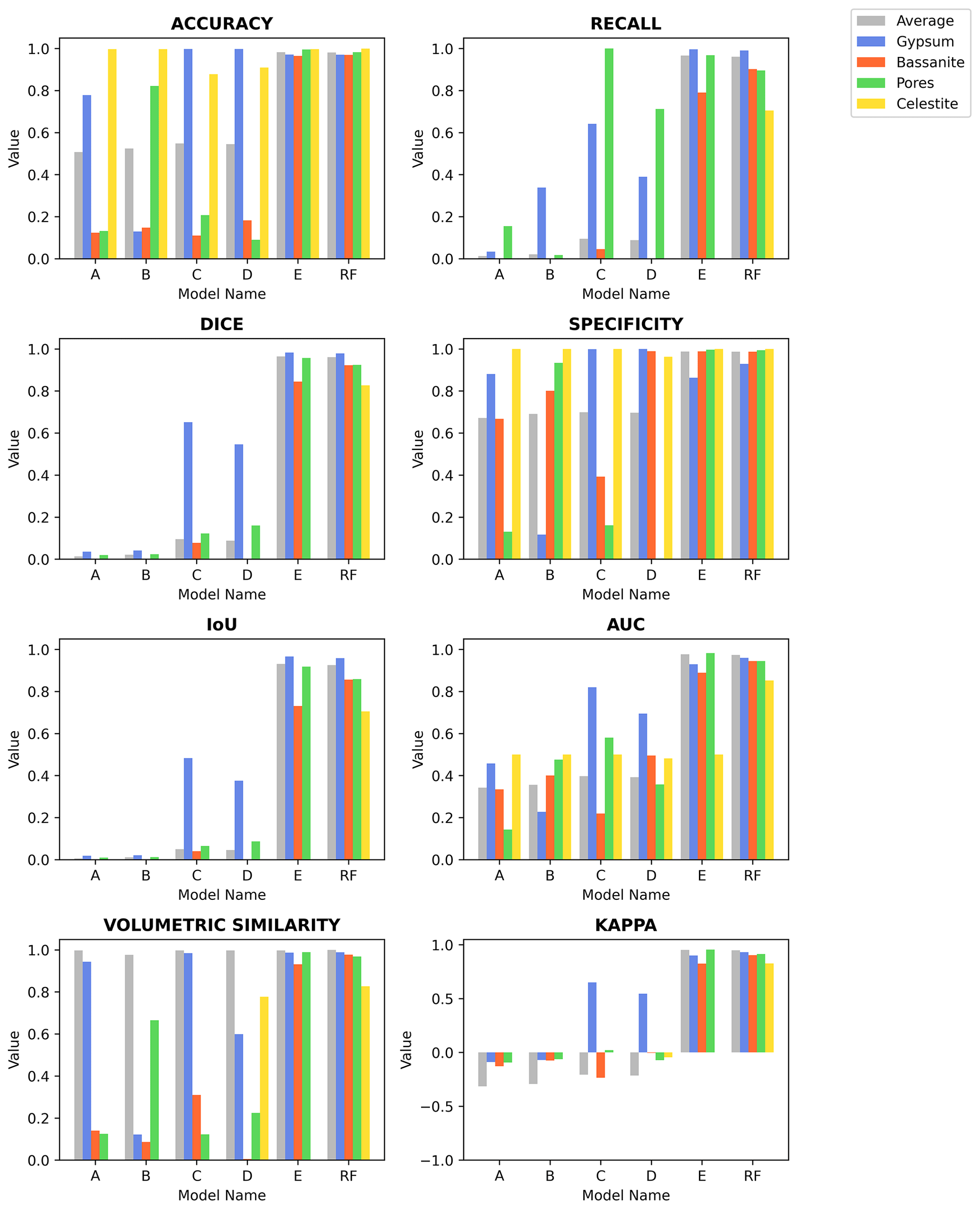
Figure C1 Eight common evaluation metrics calculated for the different segmentation models, accuracy, recall, Dice coefficient (DICE), specificity, intersection-over-union (IoU), area under the receiver operating characteristic (AUC), volumetric similarity, and Cohen's kappa (Kappa), are evaluated for the average volume and for each of the phases present in the analysed sample volume. Please refer to the main text for details regarding each trained model.

C2 Accuracy

Accuracy is one of the best-known evaluation metrics in statistics (Müller et al., 2022). It is defined as the number of correct predictions, consisting of true positives and true negatives, compared to the total number of predictions. However, many recent works (see Taha and Hanbury, 2015; Müller et al., 2022, for a complete review) have discouraged the use of accuracy in image analysis, particularly in multi-class segmentation where class imbalance is highly common; because of the true negative inclusion, the accuracy metric will always result in an anomalous high scoring (Müller et al., 2022). This can be clearly seen in Fig. C1, where the score for the Accuracy metric is high also for those models which do not perform well if taking into account other metrics. Accuracy is calculated as follows:

$$\begin{array}{}\text{(C4)}& \text{Accuracy }={\displaystyle \frac{\mathrm{TP}+\mathrm{TN}}{\mathrm{TP}+\mathrm{TN}+\mathrm{FN}+\mathrm{FP}}}.\end{array}$$

C3 F-measure-based metrics

F-measure, also known as F-score, metrics are among the most widely used evaluation performance metrics for computer vision and image analysis (Taha and Hanbury, 2015; Müller et al., 2021, 2022; Allen et al., 2022). It is calculated from recall and precision of a prediction, by which it scores the overlap between predicted segmentation and ground truth. Including the precision metric, F-measure penalises false positives, which can be common features in multi-class datasets – such as those derived from X-ray μCT. There are two metrics based on the F-measure: Dice coefficient, also called F1 or the Sørensen–Dice index, and the intersection-over-union (IoU), also known as the Jaccard index or Jaccard similarity coefficient. The Dice coefficient is defined as the harmonic mean between sensitivity and precision and is calculated as follows:

$$\begin{array}{}\text{(C5)}& \mathrm{DICE}={\displaystyle \frac{\mathrm{2}\cdot \mathrm{TP}}{\mathrm{2}\cdot \mathrm{TP}+\mathrm{FP}+\mathrm{FN}}}.\end{array}$$

The IoU, instead, is defined as follows:

$$\begin{array}{}\text{(C6)}& \mathrm{IoU}={\displaystyle \frac{\mathrm{TP}}{\mathrm{TP}+\mathrm{FP}+\mathrm{FN}}}.\end{array}$$

We can also define DICE as follows:

$$\begin{array}{}\text{(C7)}& \mathrm{DICE}={\displaystyle \frac{\mathrm{2}\times \mathrm{IoU}}{\mathrm{1}\times \mathrm{IoU}}}.\end{array}$$

C4 Area under the receiver operating characteristic

The receiver operating characteristic (ROC) is a line plot of the diagnostic ability of a classifier by visualising its performance with different discrimination thresholds (Taha and Hanbury, 2015; Müller et al., 2022). The performance is assessed through the true positive rate against the false negative rate. We can use the area under the receiver operating characteristic (AUC) as a single-value evaluation performance metric for the validation of image classifiers (Müller et al., 2022). The following AUC formula is determined as the area of the trapezoid defined by the ROC plot (see Müller et al., 2022 for a full formulation):

$$\begin{array}{}\text{(C8)}& \mathrm{AUC}=\mathrm{1}-{\displaystyle \frac{\mathrm{1}}{\mathrm{2}}}\left({\displaystyle \frac{\mathrm{FP}}{\mathrm{FP}+\mathrm{TN}}}+{\displaystyle \frac{\mathrm{FN}}{\mathrm{FN}+\mathrm{TP}}}\right).\end{array}$$

It needs to be noted that an AUC value of 0.5 is indicative of a random classifier.

C5 Volumetric similarity

As the name suggests, volumetric similarity (VS) is a measure that considers the volume of the segmented classes to indicate similarity. Here we use the definition reported in Taha and Hanbury (2015), namely the absolute volume difference divided by the sum of the compared volumes. Taha and Hanbury (2015) define the VS as 1-VD, where VD is the volumetric distance:

$$\begin{array}{}\text{(C9)}& \text{Volumetric\hspace{0.17em}\hspace{0.17em}Similarity }=\mathrm{1}-{\displaystyle \frac{|\mathrm{FN}-\mathrm{FP}|}{\mathrm{2}\cdot \mathrm{TP}+\mathrm{FP}+\mathrm{FN}}}.\end{array}$$

C6 Cohen's kappa

This metric is defined as a change-corrected measure of agreement between ground truth and predicted classification (Taha and Hanbury, 2015; Müller et al., 2022). Differently for previous metrics, Cohen's kappa (Kappa) ranges from −1 (worst) to +1 (best); a KAPPA close to 0 indicates a random classifier. The KAPPA evaluation metric is calculated as follows:

$$\begin{array}{}\text{(C10)}& {\displaystyle }& {\displaystyle }{f}_{\mathrm{c}}={\displaystyle \frac{(\mathrm{TN}+\mathrm{FN})(\mathrm{TN}+\mathrm{FP})+(\mathrm{FP}+\mathrm{TP})(\mathrm{FN}+\mathrm{TP})}{\mathrm{TP}+\mathrm{TN}+\mathrm{FN}+\mathrm{FP}}},\text{(C11)}& {\displaystyle }& {\displaystyle }\text{Kappa}={\displaystyle \frac{(\mathrm{TP}+\mathrm{TN})-f_{\mathrm{c}}}{(\mathrm{TN}+\mathrm{TN}+\mathrm{FN}+\mathrm{FP})-f_{\mathrm{c}}}}.\end{array}$$

In the main text the Dice coefficient (Fig. 4 and Table 1) is used to evaluate and compare the segmentation resulting from the neural network trained using ground truth data derived from (i) histogram segmentation (Models A–C), (ii) histogram segmentation with data augmentation (Models D and E), and finally (iii) a random forest classifier. A complete description of all calculated metrics can be found in Fig. C1 and in Table S1 in the Supplement. Both the figure and the table report the calculated values for the different phases (gypsum, bassanite, pores, and celestite) and the average over the segmented volume for the reference volume VA19-040 (736 voxel × 800 voxel × 400 voxel). It can be noted how the introduction of data augmentation benefits the segmentation of most phases with respect to almost all metrics (particularly for Model E). However, only Model RF (trained with a random forest ground truth) includes the celestite phase (yellow in the graphs) in addition to the overall best performance in all most metrics.