the Creative Commons Attribution 4.0 License.
the Creative Commons Attribution 4.0 License.
 | 22 Jul 2024
Extraction of pre-earthquake anomalies from borehole strain data using Graph WaveNet: a case study of the 2013 Lushan earthquake in China
Chenyang Li
Yu Duan
Ying Han
Zining Yu
Dewang Zhang
On 20 April 2013, Lushan experienced an earthquake with a magnitude of 7.0. In seismic assessments, borehole strainmeters, recognized for their remarkable sensitivity and inherent reliability in tracking crustal deformation, are extensively employed. However, traditional data-processing methods encounter challenges when handling massive dataset-s. This study proposes using a Graph WaveNet graph neural network to analyze borehole strain data from multiple stations near the earthquake epicenter and establishes a node graph structure using data from four stations near the Lushan epicenter, covering the years 2010–2013. After excluding the potential effects of pressure, temperature, and rainfall, we statistically analyzed the pre-earthquake anomalies. Focusing on the Guza, Xiaomiao, and Luzhou stations, which are the closest to the epicenter, the fitting results revealed two acceleration events of anomalous accumulation that occurred before the earthquake. Occurring approximately 4 months before the earthquake event, the first acceleration event indicated the pre-release of energy from a weak fault section. Conversely, the acceleration event observed a few days before the earthquake indicated a strong fault section that reached an unstable state with accumulating strain. We tentatively infer that these two anomalous cumulative accelerations may be related to the preparation phase for a large earthquake. This study highlights the considerable potential of graph neural networks in conducting multistation studies of pre-earthquake anomalies.
- Article
(6204 KB) - Full-text XML
- BibTeX
- EndNote


Earthquakes result from the accumulation of stress in the Earth's crust during plate movement and collisions. Once the stress surpasses a critical threshold, the crust ruptures, unleashing seismic waves that reverberate through the ground, causing substantial damage (Campbell et al., 2020; Fan et al., 2021). Extensive research on earthquakes has generated a wealth of information worldwide, establishing a robust database for studying pre-earthquake anomalies.
On 20 April 2013, at 08:02 UTC, an earthquake with a magnitude of 7.0 struck Lushan County, Ya'an, Sichuan, China, within the Longmenshan fault zone. The epicenter was located at approximately 30.30° N and 103° E within the Longmenshan fault zone at a depth of 13 km. The earthquake mechanism solution revealed a retrograde rupture of the earthquake-induced rupture. By 24 April 2013, the earthquake had triggered over 4000 aftershocks, affecting more than 300 000 people across an expansive area exceeding 12 000 km2. The aftermath brought about a significant loss of life and property. Additionally, the seismic event triggered various geological hazards, such as earth fissures, landslides, and surface deformation (Hong et al., 2013).
Researchers around the world have examined various phenomena preceding and following earthquakes, delving into subterranean, surface, and spatial changes. Chen et al. (2014) studied the coseismic ionospheric anomalies of the Lushan earthquake. Guo and Zheng (2022) calculated and analyzed the anomalies of background noise near the pre-earthquake epicenter of the Lushan earthquake. Q. Liu et al. (2014) analyzed the aerosol optical depth (AOD) and concluded that the AOD could be a potential earthquake precursor in the Sichuan Basin. C. Liu et al. (2014) examined groundwater anomalies and identified medium-term dynamics and short-term or impending anomalies in solid tidal aberrations of the water level. Ma et al. (2015) analyzed pre-earthquake tidal cycles and concluded that celestial tidal forces trigger earthquakes under critical rock fragmentation and sliding conditions. Zhang et al. (2016) explored thermal anomalies as a precursor to earthquakes using a time series of surface temperatures obtained prior to the Lushan earthquake. Zhu et al. (2013) analyzed the tectonic deformation and energy accumulation in the southern section of the Longmenshan fracture zone through mobile gravity observation data. Jiang et al. (2013) found severe negative anomalies before and on the day of the earthquake by analyzing anomalies in the vertical total electron content (VTEC) in the ionosphere.
Based on findings from the Plate Boundary Observation (PBO) project proposal from the United States, borehole strain observations have emerged as superior to GPS and laser strainmeters in capturing short- to medium-term strain variations and pre-earthquake strain variations (Zhang, 2004; Zheng and Zhang, 2004). China has deployed multiple four-component YRY-4 borehole strainmeters, offering not only four-component data but also auxiliary observations of air pressure, groundwater level, and temperature (Chi et al., 2007; Qiu, 2014; Qiu et al., 2020). Numerous studies on the Lushan earthquake have employed borehole strain data. Qiu et al. (2013) correlated borehole strain data from the Guza station with other influencing factors before the Ms 7.0 earthquake in Lushan, establishing a connection to the earthquake. Zhu et al. (2018) identified the precursors of the Lushan earthquake by analyzing the eigenvalues and eigenvectors from borehole data. Yu et al. (2021) employed a state-space model to decompose the strain into component responses and discovered the synchronous acceleration of negative-entropy anomalies at multiple stations 4 to 6 months before an earthquake. Liu et al. (2019) used the S-transform method to analyze the time–frequency characteristics of borehole strain data, revealing reliable anomalies that reflect the entire process of pre-earthquake, mid-earthquake, and post-earthquake strain changes. Chi (2013) uncovered a phenomenon of “tidal aberration”, persisting over 3 months before the earthquake, with significant strain changes occurring 15 to 19 d prior to the earthquake. Tang and Jing (2013) conducted an analysis of surface strain coseismic orders, noting differences between the Wenchuan and Lushan earthquakes related to earthquake magnitude. Despite the valuable insights gained, these studies mostly focused on single-station data, overlooking the potential correlations between multiple stations. The study of seismic-monitoring data from multiple stations has been applied to many scenarios. Liu et al. (2019) analyzed the abnormal fluctuations in aerosol optical depth (AOD) that occurred before and after the 2008 Wenchuan earthquake and the 2013 Lushan earthquake and found that abnormally high AOD values appeared 11 d before the Wenchuan earthquake and 4 d before the Lushan earthquake. It has been considered that the AOD index may be suitable as a precursor to earthquakes in the Sichuan Basin. Using borehole strain data from six stations in the Sichuan–Yunnan region, Yu et al. (2020) established a graph network and analyzed 13 earthquake cases with Es>107 in the study area, where the Es index represents the daily total of local earthquake energy associated with the strain network. It was found that strain anomalies preceding the earthquake generally occurred within the first 30 d of the earthquake event. To study the abnormal strain changes that preceded the Wenchuan earthquake, Zhu et al. (2019) applied negative-entropy analysis to borehole data from three stations. The results show that the Guza and Xiaomiao stations exhibit similar trends and may have recorded abnormal changes related to the Wenchuan earthquake. The Renhe station failed to detect the anomalies that occurred before the earthquake due to the distance. An example of the multistation analysis is given to show that it is feasible to analyze seismic data using multiple stations.
As earthquake-monitoring data accumulate, traditional processing methods face challenges in managing vast quantities of data. The emergence of deep learning, particularly graph neural networks (GNNs), has markedly enhanced the accuracy of prediction and classification, especially regarding non-Euclidean spatial-data characterization (Kipf and Welling, 2017; Niepert et al., 2016; Scarselli et al., 2009; Wu et al., 2019; Zhou et al., 2020). Recent developments in spatiotemporal GNN frameworks have integrated GNNs with various event-learning methods to extract complex dependencies (Oord et al., 2016; Rathore et al., 2021; Yu et al., 2017). Kim et al. (2022) utilized raw waveform data from multiple stations to classify earthquake events, demonstrating the effectiveness of GNNs in aggregating features from individual stations. Bilal et al. (2022) refined earthquake magnitude, depth, and location predictions by extracting features from waveform data from multiple stations and integrating earthquake catalog information into a GNN. Huang et al. (2023) applied an Isomorphic Graph Attention Network (IsoGAT) to analyze earthquake catalogs and geomagnetic signals, successfully detecting pre-earthquake anomalies. These studies highlight the significant potential of GNNs in earthquake research.
In this study, we propose an innovative method for extracting pre-earthquake anomalies from borehole strain data using Graph WaveNet. The remainder of this article is structured as follows. The next section delves into the specifics of the Lushan earthquake, providing an introductory exploration of the observation data pivotal to our analysis. In the third section, we introduce the segmented variational modal method (SVMD) and delve into the theoretical underpinnings of the Graph WaveNet network, laying the groundwork for a comprehensive understanding of our analytical approach. A detailed case study of the Lushan earthquake follows, providing a tangible illustration that guides readers through the intricacies of our data-processing methodology. Section 5 includes the analysis of prediction results, the detailed analysis of randomly selected abnormal days, and the analysis of abnormal accumulation results. The sixth part comprises the discussion, which mainly includes the comparison and analysis of the abnormal accumulation results from different stations and the exclusion of the influence of meteorological factors. The final section presents the conclusions of the study and summarizes the key insights drawn from our analysis.
Dobrovolsky's estimate of the radius of influence of precursors for earthquakes of different magnitudes is shown in Eq. (1) (Dobrovolsky et al., 1979):
where M denotes the magnitude and ρ denotes the radius of influence of M. The radius of influence of the Ms 7.0 Lushan earthquake extends approximately 1023 km. Among the selected monitoring stations, the Guza station is situated 73 km from the epicenter, while the Xiaomiao, Luzhou, and Zhaotong stations are positioned at distances of 268, 286, and 337 km from the epicenter, respectively. This positioning confirms that the chosen stations possess the capability to monitor earthquake-related anomalies. Detailed information about the Guza, Xiaomiao, Luzhou, and Zhaotong stations, including latitude and longitude coordinates, distance from the Lushan earthquake's epicenter, rock type at the drill borehole locations, and borehole depth, is provided in Table 1. Figure 1 visually depicts the geographical locations of the four observation stations relative to the epicenter of the Lushan earthquake.
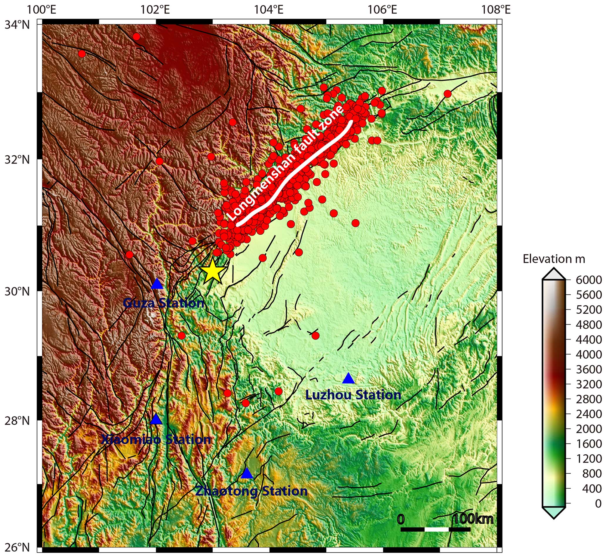
Figure 1Locations of the four observation stations relative to the epicenter of the Lushan earthquake. The blue triangles represent the locations of the borehole strain observation stations. The yellow star represents the epicenter of the Lushan earthquake, while the white curve depicts the Longmenshan fault zone. This map was generated using Generic Mapping Tools (GMT) software (version 6.0.0rc5; https://gmt-china.org/, last access: 16 June 2024).
Table 1Information on borehole strain stations was used in this study.
The four-component borehole strainmeter measures the temporal inverse of displacement at a specific point, offering insights that are not attainable through GPS and seismometers. Operating with a continuous recording frequency of one sample per minute, it significantly enhances the temporal resolution by at least 1 order of magnitude. Additionally, its observation bandwidth surpasses that of seismometers, particularly at the long-period end of the spectrum. This specialized YRY-4 strainmeter comprises four horizontally positioned sensors designed to measure changes in borehole diameters. These sensors are strategically spaced at a 45° angle, and the relationship between the four measurements from the strainmeter can be expressed as follows (Qiu et al., 2009; Su, 2019):
Eq. (2) provides the self-consistent formulation for a four-component borehole strainmeter. The self-consistent coefficient k ideally has a value of 1, and data are deemed reliable when k is greater than or equal to 0.95. Strain conversion is achieved using Eq. (3), which employs the four measurements:
In Eq. (3), S13 and S24 represent two independent shear strains. Shear strain pertains to alterations in the total area or volume of an object while maintaining a deformed shape. Additionally, Sa denotes surface strain, signifying changes in area without a concurrent shift in the object's morphology. This characteristic is observed in the presence of hydrostatic enclosure pressure (Su, 2019). For the analysis in this paper, Sa data from four stations – Guza, Xiaomiao, Luzhou, and Zhaotong – were specifically selected for examination.
Despite its advantages, such as high sensitivity and a wide frequency band during observation, the four-component borehole strainmeter remains susceptible to interference from surrounding sources. We used the improved variational-mode-decomposition (VMD) algorithm to analyze the Sa data and found that the first two components in the decomposition results correspond to the annual trend term and the solid tide, respectively, and that the remaining components contain a large number of strain signals. We retained the remaining components as research data. Because we cannot extract meteorological factors like air pressure, temperature, and rainfall from the remaining components, we analyzed the measured data of these meteorological factors to determine whether the meteorological data affect the results of the borehole strain observations.
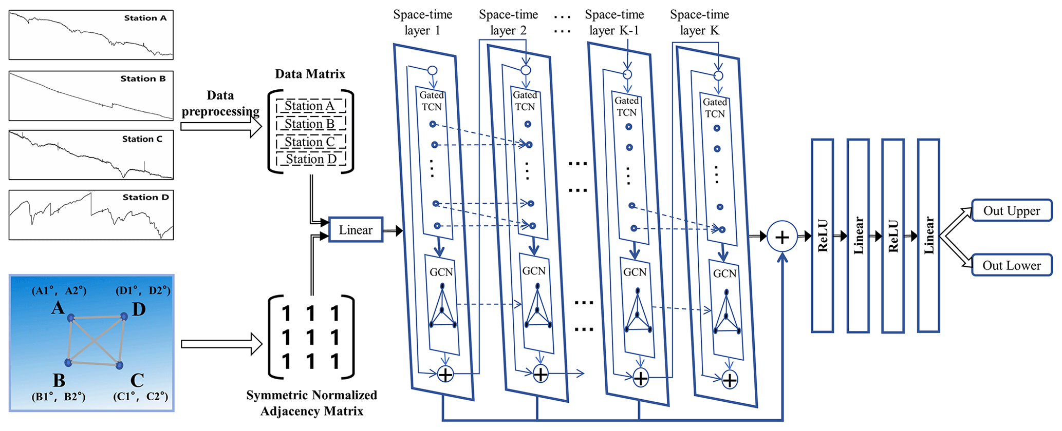
To analyze borehole strain data from multiple stations with regard to the Lushan earthquake, our study employed the flowchart shown in Fig. 2.
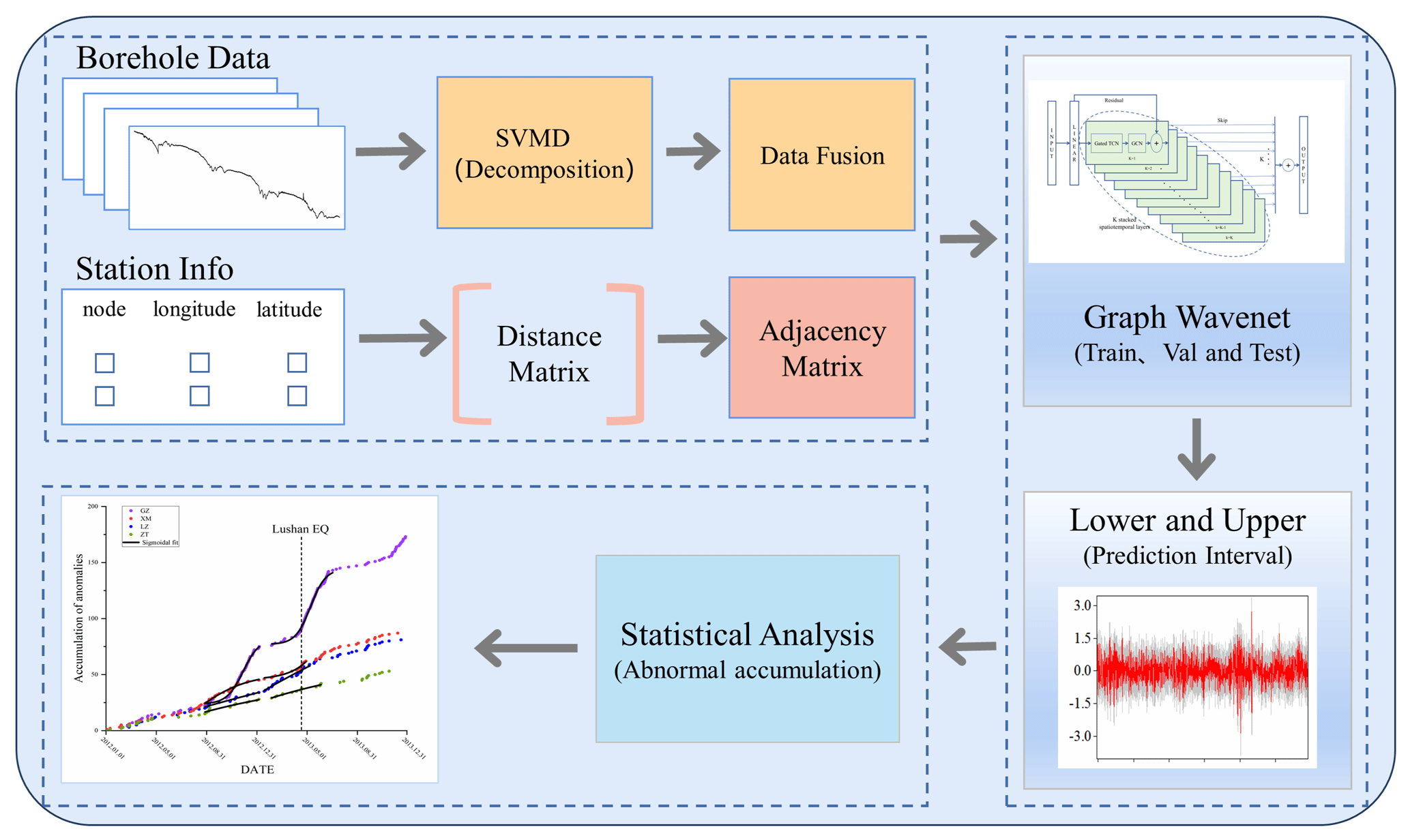
Figure 2The framework for borehole strain data processing and the detection of pre-earthquake anomalies. GZ: Guza. XM: Xiaomiao. LZ: Luzhou. ZT: Zhaotong. EQ: earthquake. TCN: temporal convolutional network. GCN: graph convolutional network.
As shown in Fig. 2, the process begins with the conversion of data from the four-component borehole into strain dataj. Subsequently, the borehole data are decomposed using the segmented variational modal method (SVMD), and the resulting decomposed outcomes are fused. By calculating the distances between stations using latitudinal and longitudinal coordinates, a distance matrix is constructed and then normalized to form an adjacency matrix. The fused data and adjacency matrix serve as inputs for training, validation, and prediction using the Graph WaveNet GNN. During the prediction phase, upper- and lower-bound prediction intervals are established based on the model's output. Anomalies are identified by comparing the prediction intervals with the original data. The cumulative values of the pre-earthquake anomalies in the borehole strain data from various stations are subsequently subjected to statistical analyses.
3.1 Segmented variational modal decomposition
A borehole strain signal, characterized as a typical nonstationary signal, can be effectively analyzed by decomposing it into a set of intrinsic mode functions (IMFs) using empirical mode decomposition (EMD). However, EMD encounters challenges, such as mode aliasing. To address this issue, an adaptive time–frequency analysis algorithm, variational mode decomposition (VMD), was introduced by Dragomiretskiy and Zosso (2014). VMD exhibits superior noise immunity in signal processing, providing an effective solution to these challenges. This approach has been successfully applied by Huang et al. (2022) and Zhang and He (2023) to process raw earthquake waveforms, yielding improved decomposition results.
VMD is a nonrecursive signal-processing method designed to decompose a time series into a sequence of IMFs characterized by a limited bandwidth. The decomposition process essentially involves solving variational problems, and the variational model can be expressed as follows:
where and are the k modal functions and the corresponding center frequencies of the signal decomposition, respectively; ∂t is the bias computation for time t; δ(t) is the unit impulse function; j is the imaginary unit; and • is the convolution computation.
To solve the variational model, a quadratic penalty term α and the Lagrange multiplier operator λ(t) are introduced to make the variational model unconstrained. The constructed generalized Lagrangian function is expressed as
where L denotes the Lagrangian generalization operator, α denotes the data fidelity constraint function, and λ denotes the Lagrange multiplier.
The alternating direction method of multipliers (ADMM) is used to solve Eq. (5) and the iterative optimization of uk, ωk, and λ. The iterative formulas for the mode uk, the corresponding center frequency ωk, and the Lagrange multiplier λ can be updated using
where is the kth IMF component in the (n+1)th iteration, is the center frequency corresponding to , is the value of the Lagrangian operator in the (n+1)th iteration, and τ is the noise tolerance of the signal. The termination condition of the algorithm is then set as follows:
where ε denotes the discrimination accuracy.
In this study, we employ a method of applying variational mode decomposition (VMD) to data segments through the incorporation of sliding windows (SVMD). This approach effectively addresses the challenge of limited memory when conducting VMD on the entire dataset while retaining the correlation between the data points (Chi et al., 2023). The fundamental principle of the SVMD method is illustrated in Fig. 3.
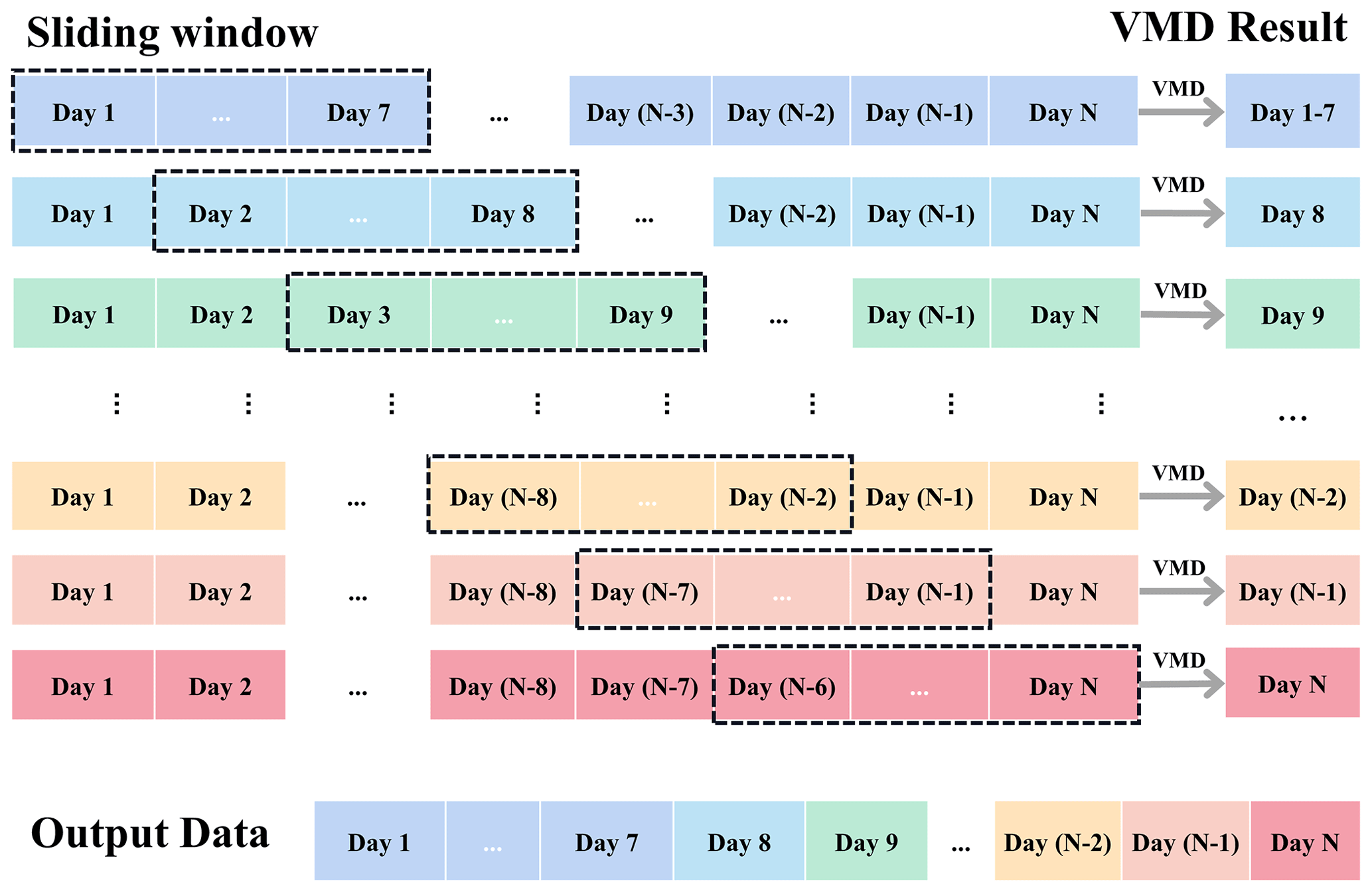
Figure 3Schematic diagram illustrating the principle of the segmented variational modal method (SVMD).
As depicted in Fig. 3, we opt for a consistent sliding-window approach with a size of 7 and a sliding step of 1. The initial sliding window encompasses all the data from the first 7 d. From the second sliding window onwards, only the data from the last day of the current window are preserved and appended to the results obtained from the previous window.
3.2 Graph WaveNet neural network architecture
3.2.1 Gated temporal convolutional network for extracting temporal features
During the processing of the time-series data, causal convolution maintains the causal relationships inherent within the data. This technique facilitates the extraction of time-series features through convolution. However, as the sequence length increases, capturing temporal dependence requires more convolution layers, thereby substantially increasing computational demands. To address this challenge, an expansion factor was introduced for causal convolution. The inclusion of this expansion factor can enlarge the receptive field of causal convolution, enabling the capture of longer time-series features with a reduced number of convolutional layers. The relationship between the input sequence length Lin after causal dilation convolution and the output sequence length Lout can be expressed as
where Lout is the length of the output sequence; Lin is the length of the input sequence; padding is the number of zeros added to the end of the input sequence (and added to the beginning of the sequence to preserve causality); k is the size of the convolution kernel, which is a small, learnable weight matrix; and d is the dilation factor, which indicates the span of the convolution kernel across the input sequence, with larger dilation factors capturing long-term time dependencies. The dilation causal convolution with a convolution kernel size of 2 and a sliding step of 1 is shown in Fig. 4a.

Figure 4(a) Schematic of the dilated causal convolutional layers. (b) Architecture of the spatiotemporal layers.
Although convolutional neural networks (CNNs) are commonly employed in image processing, 1D CNNs can also be effectively used in time-series analysis. Gated temporal convolutional networks (TCNs) leverage 1D CNNs to extract features from time-series data. This architecture comprises two key modules: one for convolving the input data to extract features by employing tanh as the activation function and the other for controlling the amount of information passed from the current layer to the next layer by utilizing the sigmoid activation function. The gated TCN module is defined as
where W1 and W2 represent the weight parameters, b1 and b2 represent the corresponding bias parameters, • denotes the convolution, g is the activation function of the output, and σ is the activation function that determines the ratio of information passed to the next layer.
3.2.2 Graph convolutional networks (GCNs) for extracting spatial features
The fundamental concept of a graph network is to represent interactions among real features based on spatial dependence dictated by the graph structure. The distance–adjacency matrix is symmetrically normalized to function as an adjacency matrix for graph convolution. This approach effectively captures the node information and preserves the graph structure. By constructing a complete undirected graph for each station, where all nodes are directly connected, each node interacts solely with its neighboring nodes to exchange information. To ensure that the input features captured all information from the current node and its first-order nearest-neighbor nodes, a first-order symmetric normalized adjacency matrix was selected during the graph convolution process. The convolution layer of the graph is defined as
where H(l) denotes the embedding vector of layer l, H(l+1) denotes the embedding vector of layer (l+1), denotes the symmetric normalized adjacency matrix of the current layer, D denotes the degree matrix, denotes the distance–adjacency matrix, W(l) denotes the weight of the neural network in the current convolutional layer, and σ denotes the nonlinear activation function of the neural network. Introducing a dropout rate to the output of each training batch in the graph convolution process involves randomly ignoring half of the hidden-layer nodes.
This dropout strategy was applied across different neural networks, and “opposite” fits were averaged. This aids in mitigating overfitting because conflicting tendencies can cancel each other out during the training process.
3.2.3 Spatiotemporal layers
Figure 4b illustrates the structure of the spatiotemporal layer. Each layer within the spatiotemporal layer captures temporal dependencies using gated TCNs. This involves utilizing node features produced by the TCN module and the graph's adjacency matrix as inputs for the GCN module. The GCN layer is responsible for capturing spatiotemporal features, and the spatiotemporal features of the current layer are residual and linked to the input, serving as inputs for the subsequent spatiotemporal layer. The output of the gated TCN module serves as the output of the current spatiotemporal layer, and the outputs of all spatiotemporal layers are interconnected using skip connections. This design facilitates the capture of short-term and spatial dependencies.
3.2.4 Graph WaveNet neural network framework
Figure 5 illustrates the framework of Graph WaveNet. The initial step involves pre-processing the multistation borehole data and converting the latitude and longitude data of each station into an adjacency matrix. Subsequently, the data undergo an increase in dimensionality in the linear layer, followed by processing in the gated TCN module, to obtain the current information. The output of the gated TCN module is then employed to extract spatial information through the GCN layer. The extracted spatial and temporal information is connected to the input of the current layer, which serves as the input for the subsequent spatial and temporal layers; this input can capture both current and historical information using different dilation factor sizes. Finally, the information extracted from each gated TCN layer is aggregated into an output layer. The output sequence is downscaled using the rectified-linear-unit (ReLU) activation function and a linear layer. The upper and lower bounds of the output sequence are calculated using the normal-distribution method. The prediction intervals of the network are constructed from the upper and lower bounds. The upper and lower bounds of the prediction intervals are determined using the following formulas:
where Prediction is the predicted value; Z is the Z score of the normal distribution, which is about 1.96 for a 95 % confidence level; and RMSE is the root mean square error.
For the Graph WaveNet neural network model, the mean absolute error (MAE) was employed as the loss function for backpropagation during training. A dropout of 0.3 was applied during graph convolution to enhance the model's generalization. The Adam optimizer was utilized to update the weights, with a learning rate of 0.001 and a weight decay rate of 0.0001. This configuration allowed the model to decay, effectively preventing overfitting by reducing the parameter magnitudes. The number of training rounds for the model was set to 100.
We analyzed the four-component borehole strain data collected from the Guza, Xiaomiao, Luzhou, and Zhaotong stations from 1 January 2010 to 31 December 2013. Initially, the data from each station were validated using self-consistent equations. Subsequently, the four-component borehole strain data from each station were transformed into two shear strains, S13 and S24, and one surface strain, Sa, using a strain conversion equation. Figure 6a shows the data series for surface strain Sa data after converting the borehole strain data from each of the four stations.
Subsequently, the Sa data from each of the four stations were decomposed using the segmented variational modal method (SVMD). The decomposition parameters were set to a bandwidth of 2000, five modes were selected for decomposition, and the convergence accuracy was set to 10−7. The results of the SVMD decomposition were compared with data related to the influencing factors to effectively eliminate the effects of seasonal trends and solid tides. The extracted modes are specifically related to crustal activity, showcasing short-period, high-frequency oscillatory signals associated with variations in earthquake strain within crustal motions (Chi et al., 2019). The time-series data obtained after the SVMD decomposition of Sa data from each station are illustrated in Fig. 6b.
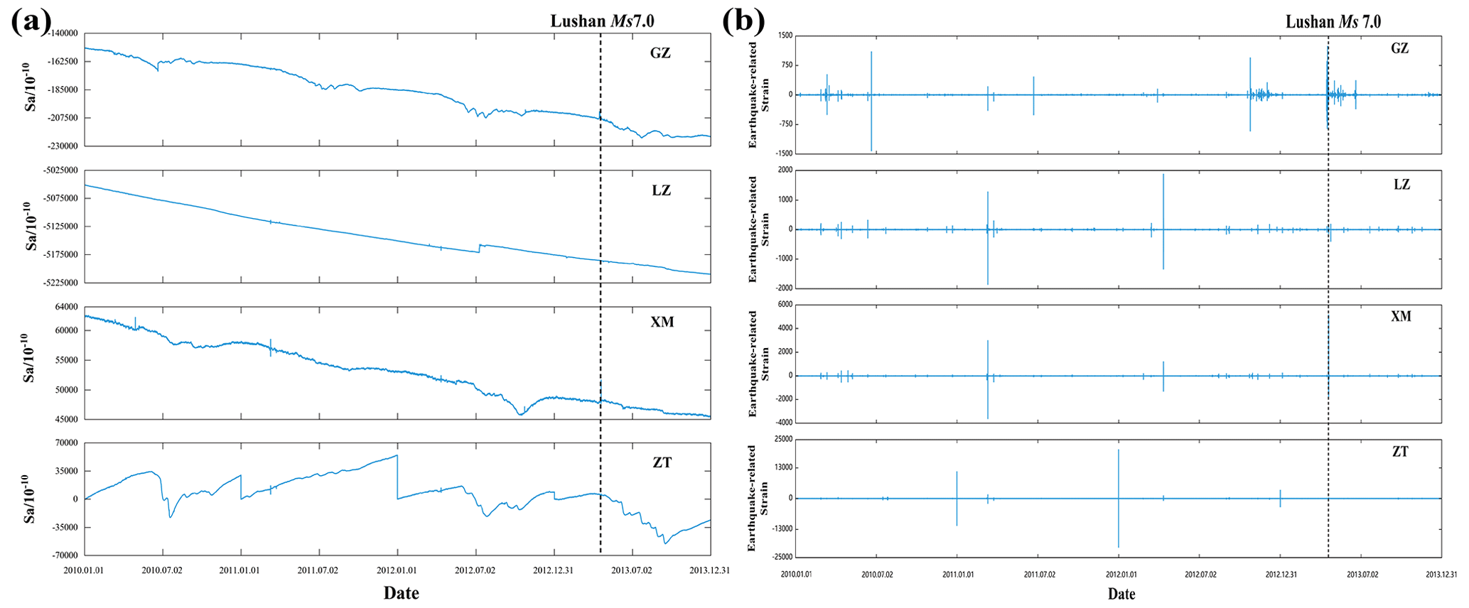
Figure 6(a) Sa of the borehole strain data from 2010 to 2013 for the Guza, Xiaomiao, Luzhou, and Zhaotong stations. (b) SVMD results for the Sa components at the Guza, Xiaomiao, Luzhou, and Zhaotong stations.
The next step involved data fusion, in which the SVMD was applied to the Sa component data from different stations to extract data related to crustal activities. The construction of the GNN required information from each node; hence, data from multiple stations were fused as inputs to the GNN. The data matrix Ra of the constructed Ra component is given by
where GZ, LZ, XM, and ZT represent the Guza, Luzhou, Xiaomiao, and Zhaotong stations, respectively; a denotes the selection of the Sa component data; t denotes the length of the time series; and T denotes the transpose; and the fused-data matrix R serves as the input for the node information in the Graph WaveNet GNN. The constructed data matrix has a minute-level sampling interval with 1440 data sampling points per day. The data matrix undergoes processing using a sliding window with a length of 60, corresponding to 1 h. This sliding window was implemented to predict data for the next hour based on data from the current hour. The sampled data are considered the features of the sample, and the data shape is constructed as a tensor of [64, 60, 4, 1], where 64 denotes the sample length and [60, 4, 1] represents the input or output of a single data point. In this context, 60 signifies the sequence length, 4 represents the number of nodes, and 1 represents the number of node features. The selected data spanned the years from 2010 to 2013 and were divided chronologically into a ratio of . Specifically, the 2010 and 2011 datasets were used as the training and validation sets, respectively, whereas the 2012 and 2013 datasets were used as the test sets.
The subsequent step involved constructing the adjacency matrix of the graph. A node graph of the four stations is shown in Fig. 7. The graph is defined as , where V corresponds to the set of nodes and E corresponds to the set of edges in the graph. The relationship between the edges and nodes is expressed as Eij=(ViVj), Vi, Vj∈V. Graphs are commonly represented using an adjacency matrix, where the adjacency matrix A is an N×N square and N denotes the number of nodes. The graph is expressed as Aij=1 if vertices i and j are connected by an edge and expressed as Aij=0 otherwise. The number of neighboring nodes for node V is referred to as the degree of said node, and the degree matrix D is an N×N diagonal array, with diagonal elements representing the degrees of individual vertices – i.e., D(Vi)=N(i).
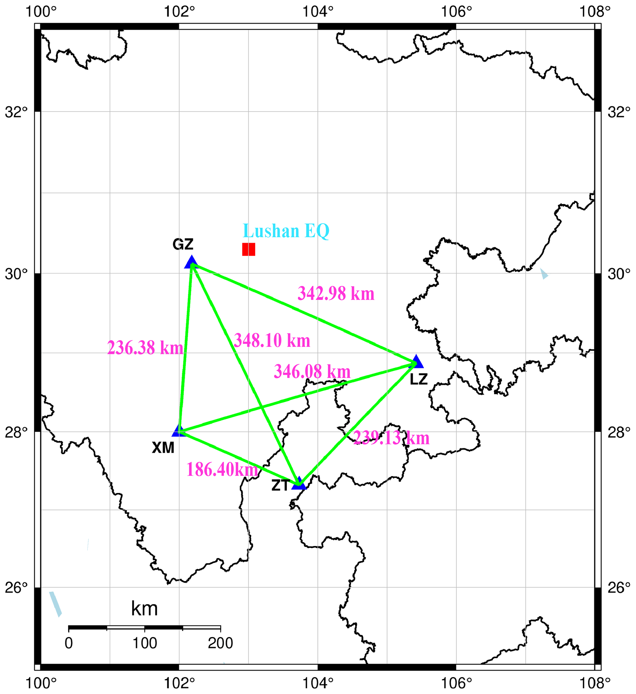
Figure 7Node diagram illustrating the four borehole strain observation stations. The blue triangles indicate the locations of the four borehole strain stations, the green lines indicates the distances between the pairs of stations, and the red square indicates the epicenter of the Lushan earthquake.
The true distance between the stations was calculated using the corresponding latitude and longitude data of any two stations. Assuming that the Earth is a standard sphere, the principle for calculating the distance using latitude and longitude coordinates involves determining the distance between two points on the sphere, which is equivalent to the arc length of a cross-sectional circle. For any two given points with corresponding latitudes and longitudes, A(N1,E1) and B(N2,E2), where R represents the average radius of the Earth and the center of the Earth is assumed to be the midpoint of the right-angle coordinates, A and B represent two points corresponding to the following right-angle coordinates:
We calculated the angle between two points based on the coordinates of points A and B. When the angle between A and B is α, the cosine of the angle cosα is calculated as follows:
Thus, the distance d between two points can be expressed as
The distance between two stations was determined by calculating the latitude and longitude coordinates of any two stations. Subsequently, a distance–adjacency matrix for the node graph was constructed based on these distances. To optimize the adjacency matrix for use in the Graph WaveNet GNN, the distances between the nodes were normalized to represent the weights between them. This normalized adjacency matrix was then utilized in the Graph WaveNet model.
In this study, we employed a Graph WaveNet GNN to analyze borehole data from multiple stations collected prior to the Lushan earthquake. The analysis focused on extracting pre-earthquake anomalies based on the results obtained. Anomalies were identified when the raw data surpassed the corresponding upper or lower prediction intervals established by the network. The prediction results for each station are shown in Fig. 8.
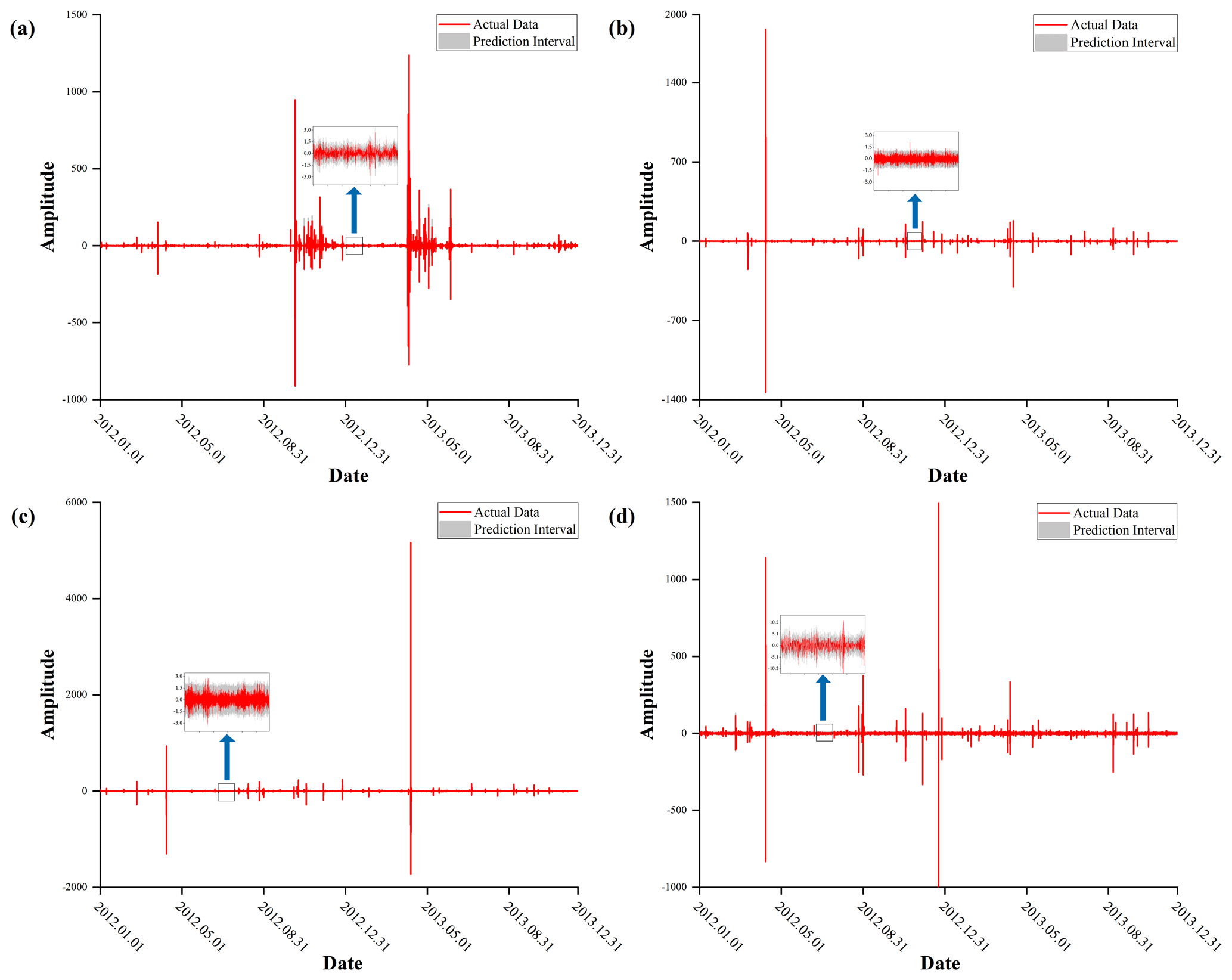
Figure 8Prediction results from the Graph WaveNet GNN. The red lines indicate real data, and the gray areas indicate prediction intervals. (a) Results of the Lushan earthquake prediction from the Guza station. (b) Results of the Lushan earthquake prediction from the Luzhou station. (c) Results of the Lushan earthquake prediction from the Xiaomiao station. (d) Results of the Lushan earthquake prediction from the Zhaotong station.
As shown in Fig. 8, our raw data closely align with the predicted intervals, demonstrating that the Graph WaveNet GNN accurately predicted the borehole data at each station. To identify point anomalies in the borehole strain data predictions, we employed the following criteria: (a) detecting more than 15 points outside the intervals within a 30 min window and (b) identifying differences between the center of the predicted intervals and the actual values exceeding 1.5 times the bandwidth of the intervals (with more than three such points occurring in the same 30 min period). Days meeting these conditions were considered anomalous (Chi et al., 2023). To validate whether the extracted anomalous days were related to earthquakes, we randomly selected raw data for four anomalous days from each station, as shown in Fig. 9.
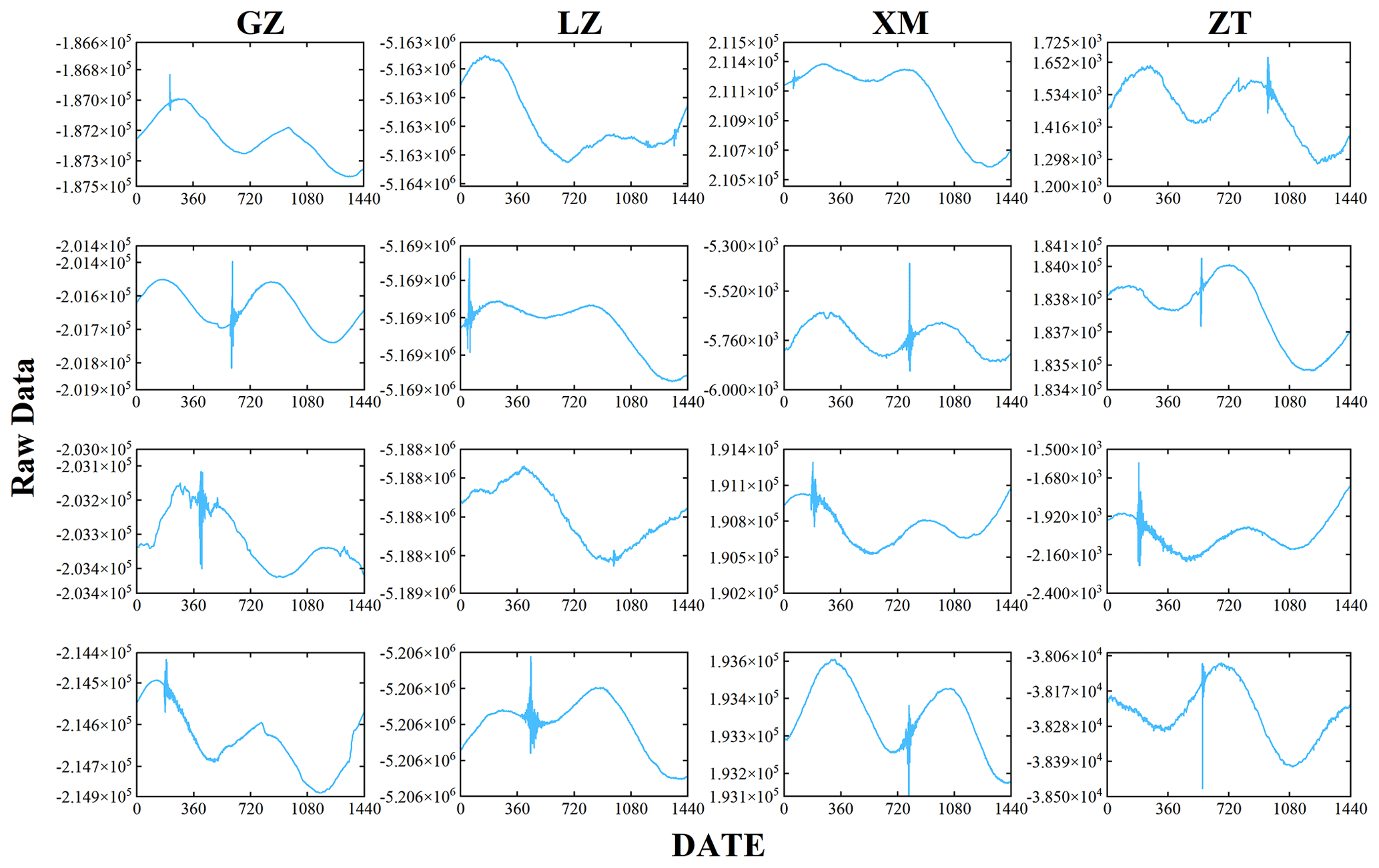
Figure 9Plots illustrating raw data from four randomly selected anomalous days at each station.
In Fig. 9, it is evident that the abnormal days we defined exhibit short-period, high-frequency oscillation signals in the original waveform, suggesting that these days are associated with crustal activity. De Santis et al. (2017) studied the 2015 Nepal event using magnetic satellite data from the Swarm mission. For the first time, an S-shaped fitting function was proposed for the analysis of the abnormal accumulation, and some abnormal differences were found in the area around the earthquake epicenter based on the abnormal accumulation results. By comparing the S-shaped fitting function with the linear fitting, it was found that the S-shaped fitting function was significantly better. In this paper, the S-shaped fitting function is used to fit the abnormal accumulation results. The cumulative values of the anomalous days over time are depicted in Fig. 10.
As depicted in Fig. 10a, the cumulative results from the anomalous days at the Guza station exhibit a two-part concavity. One part displays a rapid increase in the number of anomalous days from October 2012 to 3 months before the earthquake (January 2013), after the trend levels off. Our findings align with those of Chi et al. (2013) and Zhu et al. (2018), indicating that strain anomalies occurred during the 4–8 months preceding the earthquake, with the accumulation of anomalous days exhibiting an accelerating trend. In the other part, there is a rapid increase in the number of anomalous days from March 2013 until June after the earthquake, after which the increasing trend in anomalous days gradually levels off. Relevant researchers have studied the short-term anomalies that occurred before the Lushan earthquake and believe that these anomalies occurred within a few days to a month before the earthquake (An et al., 2013; Jiang et al., 2013; Yu et al., 2020; Qiu et al., 2013; Zhu et al., 2018). Our study yielded similar results, indicating that anomalies were present in the 1-month period prior to the Lushan earthquake. Therefore, we posit that these anomalies might be related to the Lushan earthquake. The findings of Yu et al. (2021), who observed a brief increase in anomalies followed by a return to a steady state in the 2-month period after the earthquake, align closely with the outcomes of our study. Li et al. (2017) analyzed the pre-earthquake anomalies of the Lushan earthquake using seismic-rate data. The synthesized results show an anomaly of rising earthquake frequency over time that lasts for 3–5 months from September 2010, which is highly consistent with our observed rapid increase in anomalous days about 6 months before the earthquake. It indicates that we effectively extracted short-term strain precursor anomalies associated with the Lushan earthquake.
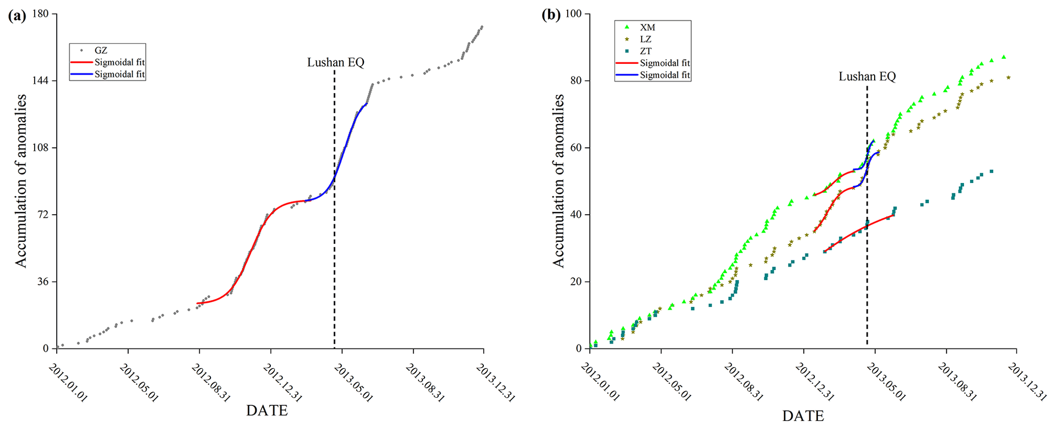
Figure 10Accumulation results for anomalous days in the borehole data from each station. The dashed line indicates the date of the earthquake, while the red and blue curves indicate the results of the S-shaped fitting function before and after the earthquake, respectively. (a) Accumulation results for anomalous days at the Guza station; (b) Accumulation results for anonymous days at the Xiaomiao, Luzhou, and Zhaotong stations.
The findings of this study align with the concept of the synergism process of a fault. Ma and Guo (2014) conducted a laboratory modeling study on the instability of a planar strike-slip fault, suggesting that the occurrence of an earthquake is linked to a fault's synergistic process, which encompasses three stages. In the initial stage, there is a deviation of the stress curve from linearity. The second stage is marked by the steady increase and expansion of isolated areas of strain release. In the final stage, the sections of strain release on the fault accelerate and expand, accompanied by a rapid increase in strain levels in areas of strain accumulation. The period from September to December 2012 corresponds to the first and the second stages, where the stress curve deviates from linearity and isolated areas of strain release grow and extend steadily. The period from early 2013 until the earthquake aligns with the third stage, characterized by the accelerated expansion of strain release sections on the fault and a swift rise in strain levels in areas of strain accumulation. The multitude of anomalies observed after the earthquake, including those caused by crustal fractures and aftershocks, were also evident. Similar phenomena were recorded at the XM and LZ stations, correlating with Ma's theory. Thus, we believe that the anomalous phenomena observed prior to the Lushan earthquake are related to the earthquake's gestation process.
Xu et al. (2019) used observation network data from the Global Navigation Satellite System (GNSS) to study the deformation that occurred before the Lushan earthquake and found a locking state that lasted from 5 months before the earthquake to 2 months after the earthquake. They also noted that under the locking state, strain energy continued to accumulate until the fault ruptured. When stress accumulation in the pregnant seismic zone transitions from a linear to a nonlinear accumulation stage, the resulting stress perturbations lead to changes in the additional stress and strain states at nearby strain measurement points as the degree of stress and strain accumulation increases. Rock rupture experiments and theoretical studies have shown that pre-slip occurs before fault strike-slip displacement, and the resulting stresses can lead to obvious anomalous responses at nearby stations (Li, 2002; Ma et al., 1998; Zhao et al., 1997). Zhang et al. (2020) conducted an analysis of cross-fault deformation preceding the Ms 7.0 earthquake in Lushan. Their findings revealed a considerable shift in the cross-fault deformation dynamics of the study area, which transitioned from a state of “inheritance”, conducive to stress accumulation, to a state of “reverse inheritance” more than 6 months prior to the earthquake. This shift exhibits characteristics of coordinated and accelerated fault activities, aligning with the metastable and sub-unstable states observed in the structural mechanics tests. We believe that even in a locked state, energy pre-release still occurs in the locked part of the fracture. As the strength of the rock rupture moves into the destabilization stage, the stress on the adjacent rocks before rupture shows obvious tension and compression regions. This generation of stress is related to local extension and weakening, with most of the anomalies appearing in the form of sudden jumps. In summary, our analysis suggests that 4–8 months prior to the Ms 7.0 earthquake in Lushan, the southern section of the Longmenshan rupture zone exhibited characteristics of a sub-stabilized state. This state led to the formation of relatively weak segments on the fault, contributing to an increase in the number of anomalous days potentially associated with the pre-release of energy. Simultaneously, the relatively strong fault segments experienced strain accumulation. In the days immediately preceding the earthquake, these strong segments reached a destabilized state due to the accumulated strain, ultimately facilitating the occurrence of an earthquake (Ma and Guo, 2014).
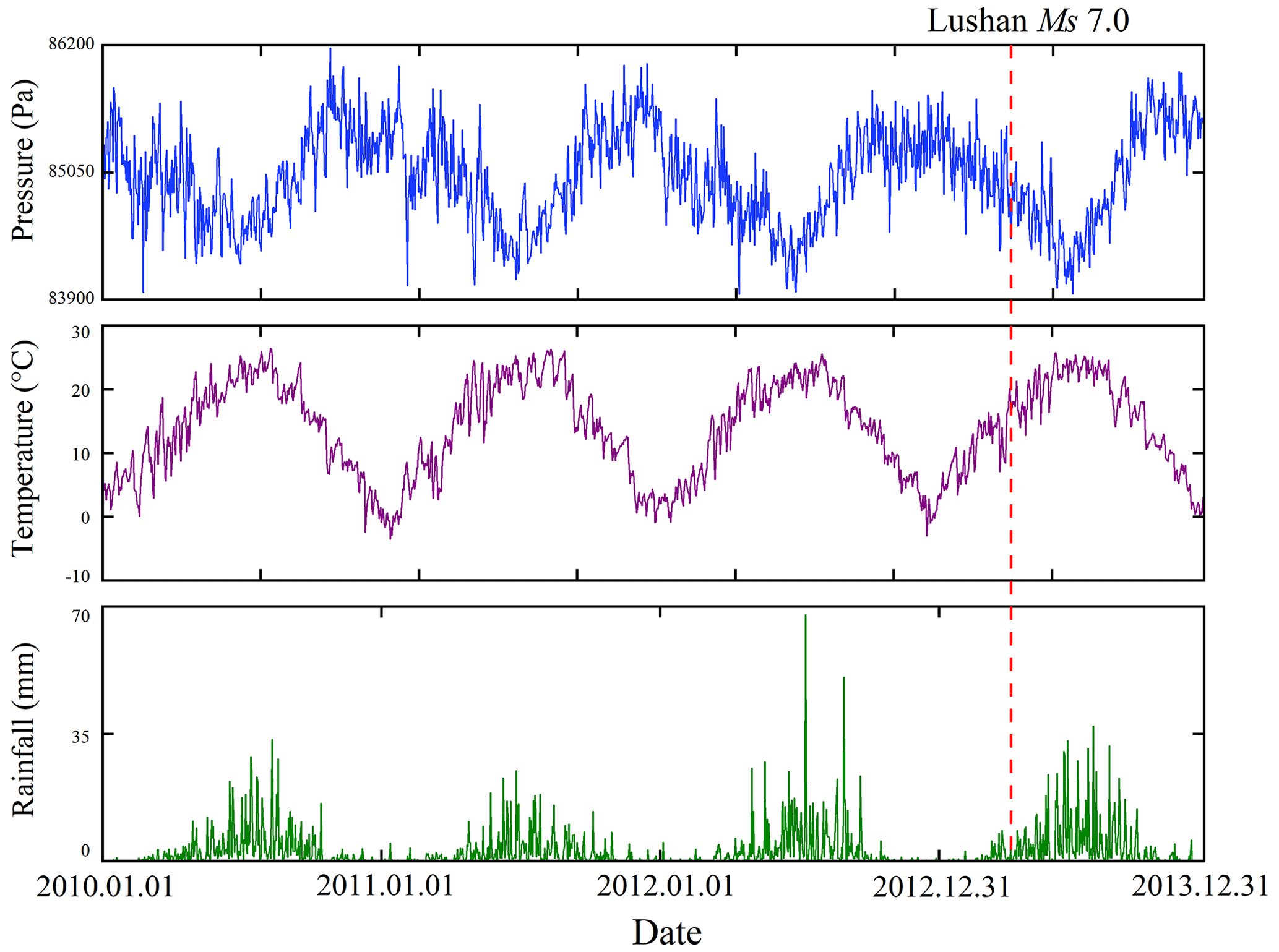
Figure 11Regional daily mean variations in pressure, temperature, and rainfall in the Lushan area from 2010 to 2013.
In Fig. 10b, we analyzed the accumulation of anomalous days at other stations within the Graph WaveNet network. Remarkably, the accumulation patterns of anomalous days at the Xiaomiao and Luzhou stations closely mirrored those observed at the Guza station, featuring concave trends in two distinct phases. However, the fitting results for the Zhaotong station deviated from the observed pattern. Analyzing these fitting results, we observed that the Xiaomiao and Luzhou stations exhibited a similar trend that resembled the patterns identified at the Guza station. In the initial phase, there was a sharp increase in January 2013, which plateaued until March 2013, indicating an accelerated accumulation of abnormal days in the 4 months leading up to the earthquake. In the second phase, from 5 April 2013 to 28 April 2013, there was a notable surge 15 d prior to the earthquake, followed by a gradual decline 8 d after the earthquake. This pattern echoes the impending and post-earthquake anomalies observed at the Guza station during the Lushan earthquake. A detailed analysis indicates that the Xiaomiao and Luzhou stations also detected anomalous signals during the gestation process of the Lushan earthquake, affirming that the anomalies at these three stations were not random but were indeed linked to the Lushan earthquake. Further scrutiny of the distances between the stations and the epicenter revealed a noteworthy pattern. The Guza station, closest to the epicenter, recorded the highest number of anomalous days, whereas the Xiaomiao and Luzhou stations, also close to the epicenter, registered fewer anomalous days than the Guza station. In contrast, the Zhaotong station, situated farther from the epicenter, reported the fewest anomalous days. This lends credence to the belief that the anomalous signals received by a station are associated with the distance between the station and epicenter.
Despite its advantages, such as high sensitivity and a wide frequency band during observation, the four-component borehole strainmeter remains susceptible to interference from surrounding sources. Figure 11 illustrates the impact of external factors by examining the regional daily mean variations in pressure, temperature, and rainfall in the Lushan region (27 to 31° N, 102 to 106° E), downloaded from 1 January 2010 to 31 December 2013 via NASA's Giovanni-4 platform (https://giovanni.gsfc.nasa.gov/giovanni, last access: 10 December 2023). The analysis of these data revealed distinct annual trends in pressure, temperature, and rainfall. Both pressure and temperature exhibited fluctuations within a certain range, displaying opposite trends, whereas rainfall underwent a consistent increase followed by a decrease each year, reflecting seasonal changes. To mitigate the impact of external factors on borehole strain data, we conducted a differencing process for the daily regional averages of pressure, temperature, and rainfall in the Lushan area. Periodic changes can be removed using differential processing, which highlights the anomalies in the data. The results are shown in Fig. 12.
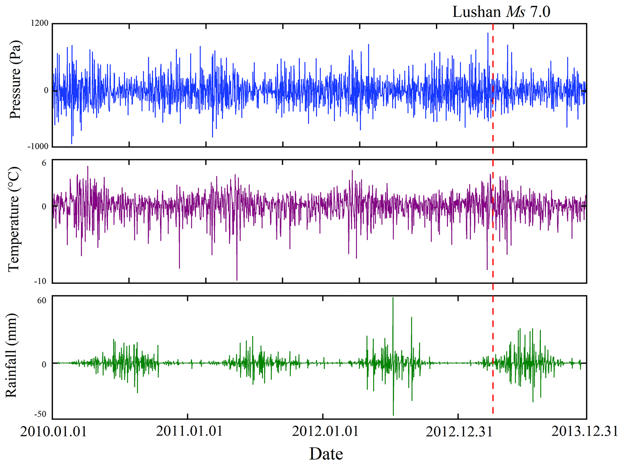
Figure 12Differing results with regard to regional daily mean variations in pressure, temperature, and rainfall in the Lushan area from 2010 to 2013.
Figure 12 indicates that the regional daily mean variations in pressure, temperature, and rainfall in the Lushan area did not exhibit any anomalous changes. Therefore, we can exclude the influence of pressure, temperature, and rainfall on the anomalies observed in the pre-earthquake borehole data from Lushan. We have reason to believe that the anomalies we extracted before the Lushan earthquake are related to the seismogenic process.
In this study, we proposed a novel method for extracting pre-earthquake anomalies based on a Graph WaveNet network structure. This method enables the integration of borehole strain data from multiple stations and makes predictions based on both temporal and spatial correlations. The statistical analysis of pre-earthquake anomalies in borehole strain data from four stations – Guza, Xiaomiao, Luzhou, and Zhaotong – revealed two S-shaped upward trends in the pre-earthquake period at the Guza, Xiaomiao, and Luzhou stations. This indicates that these three stations experienced notable strain anomalies during the gestation process of the Lushan earthquake. A comparison of anomaly accumulation rates across different stations indicated that the anomaly rate at the Guza station was substantially higher than that at the Xiaomiao and Luzhou stations, indicating a potential correlation with the distance from the epicenter. Raw-data analysis of randomly selected anomalous days from each station confirmed the correlation between the extracted anomalous days and the pre-earthquake anomalies. Additionally, we analyzed the regional daily averages of meteorological factors, preliminarily excluding their influence on the anomaly accumulation results. Therefore, we conclude that the Graph WaveNet network effectively extracted pre-earthquake anomalies from borehole strain data, highlighting its potential as a robust approach for studying pre-earthquake anomalies across multiple stations.
Data supporting the findings of this study are available from the China Earthquake Networks Center. However, restrictions apply to the availability of these data, which were used under license for the current study and are thus not publicly available. Data are, however, available from the corresponding author (email: chicqhainnu@gmail.com) upon reasonable request and with permission from the China Earthquake Networks Center.
Conceptualization: CL and CC. Data curation: CL, CC, and YD. Formal analysis: CL, CC, YH, and ZY. Investigation: CL. Methodology: CC. Resources: CC. Software: CL and DZ. Supervision: CC, ZY, and YH. Validation: CL, CC, and YH. Writing (original draft): CC and YH. Writing (review and editing): CL and CC.
The contact author has declared that none of the authors has any competing interests.
Publisher's note: Copernicus Publications remains neutral with regard to jurisdictional claims made in the text, published maps, institutional affiliations, or any other geographical representation in this paper. While Copernicus Publications makes every effort to include appropriate place names, the final responsibility lies with the authors.
The authors would like to thank Zehua Qiu, Lei Tang, and Dehe Yang from the China Earthquake Administration for their essential help in accessing the website and downloading the strain data. The authors are also grateful to Giovanni for the meteorological data (https://giovanni.gsfc.nasa.gov/giovanni, last access: 10 December 2023). The authors are also grateful to the China Earthquake Networks Center for providing the borehole strain data.
This work was supported by the Hainan Provincial Natural Science Foundation of China (grant nos. 621QN242, 622RC669, 621QN0888, 322RC659, and 320QN253) and the Program of Hainan Association for Science and Technology Plans to Youth R&D Innovation (grant no. QCXM202006). This work is supported by the Fundamental Research Funds for the Central Universities (grant no. 202213042) and the Youth Fund of the National Natural Science Foundation of China (project no. 42204005).
This paper was edited by Michal Malinowski and reviewed by two anonymous referees.
An, Z., Du, X., Tan, D., Fan, Y., Liu, J., and Cui, T.: Study on the Geo-Electric Field Variation of Sichuan Lushan MS7.0 and Wenchuan MS8.0 Earthquake, Chinese J. Geophys., 56, 721–730, https://doi.org/10.1002/cjg2.20065, 2013.
Bilal, M. A., Ji, Y., Wang, Y., Akhter, M. P., and Yaqub, M.: Early Earthquake Detection Using Batch Normalization Graph Convolutional Neural Network (BNGCNN), Appl. Sci., 12, 7548, https://doi.org/10.3390/app12157548, 2022.
Campbell, L. R., Menegon, L., Fagereng, Å., and Pennacchioni, G.: Earthquake nucleation in the lower crust by local stress amplification, Nat. Commun., 11, 1322, https://doi.org/10.1038/s41467-020-15150-x, 2020.
Chen, P., Yao, Y., Chen, J., Yao, W., and Zhu, X.: Study of the 2013 Lushan M7.0 earthquake coseismic ionospheric disturbances, Adv. Space Res., 54, 2194–2199, https://doi.org/10.1016/j.asr.2014.08.014, 2014.
Chi, C., Zhu, K., Yu, Z., Fan, M., Li, K., and Sun, H.: Detecting Earthquake-Related Borehole Strain Data Anomalies With Variational Mode Decomposition and Principal Component Analysis: A Case Study of the Wenchuan Earthquake, IEEE Access, 7, 157997–158006, https://doi.org/10.1109/access.2019.2950011, 2019.
Chi, C., Li, C., Han, Y., Yu, Z., Li, X., and Zhang, D.: Pre-earthquake anomaly extraction from borehole strain data based on machine learning, Sci. Rep., 13, 20095, https://doi.org/10.1038/s41598-023-47387-z, 2023.
Chi, S.: Strain Anomalies Before Wenchuan and Lushan Earthquakes Recorded by Component Borehole Strainmeter, Sci. Technol. Rev., 31, 27–30, https://doi.org/10.3981/j.issn.1000-7857.2013.12.004, 2013.
Chi, S., Wu, H., and Luo, M.: Discussion on strain tidal factor separation and anisotropy – Analysis of first data of borehole component strain-meter of China's digital seismological observational networks, Prog. Geophys., 22, 1746–1753, 2007.
Chi, S., Liu, Q., Chi, Y., Deng, T., Liao, C., Yang, G., Zhang, G., and Chen, J.: Borehole strain anomalies before the 20 April 2013 Lushan Ms7.0 earthquake, Acta Seismol. Sin., 35, 296–303, https://doi.org/10.3969/j.issn.0253-3782.2013.03.002, 2013.
De Santis, A., Balasis, G., Pavón-Carrasco, F. J., Cianchini, G., and Mandea, M.: Potential earthquake precursory pattern from space: The 2015 Nepal event as seen by magnetic Swarm satellites, Earth Planet. Sc. Lett., 461, 119–126, https://doi.org/10.1016/j.epsl.2016.12.037, 2017.
Dobrovolsky, I. P., Zubkov, S. I., and Miachkin, V. I.: Estimation of the size of earthquake preparation zones, Pure Appl. Geophys., 117, 1025–1044, https://doi.org/10.1007/BF00876083, 1979.
Dragomiretskiy, K. and Zosso, D.: Variational Mode Decomposition, IEEE T. Signal Process., 62, 531–544, https://doi.org/10.1109/tsp.2013.2288675, 2014.
Fan, J., Meng, J., Ludescher, J., Chen, X., Ashkenazy, Y., Kurths, J., Havlin, S., and Schellnhuber, H. J.: Statistical physics approaches to the complex Earth system, Phys. Rep., 896, 1–84, https://doi.org/10.1016/j.physrep.2020.09.005, 2021.
Guo, K. and Zheng, Y.: Big Data-based Abnormal Analysis of Seismic Background Noise before Strong Earthquake The Case of the Lushan Ms7.0 Earthquake, Earthquake Research in China, 38, 503–512, 2022.
Hong, H., Xu, H., Song, F., Zhang, X., and Li, G.: Discussion on seismo-geological hazards induced by 2013 Lushan Ms7.0 earthquake and its seismogenic fault, Acta Seismol. Sin., 35, 738–748, https://doi.org/10.3969/j.issn.0253-3782.2013.05.012, 2013.
Huang, Y., Yan, L., Cheng, Y., Qi, X., and Li, Z.: Coal Thickness Prediction Method Based on VMD and LSTM, Electronics, 11, 232, https://doi.org/10.3390/electronics11020232, 2022.
Huang, Y., Shi, W., Zhu, K. a., Qiu, H., Lu, Y., Liu, G., and Zhang, G.: A pre-seismic anomaly detection approach based on graph attention isomorphism network, Meas. Sci. Technol., 34, 125113, https://doi.org/10.1088/1361-6501/acefeb, 2023.
Jiang, W., Ma, Y., Liu, H., Deng, L., and Zhou, X.: Investigation of Lushan earthquake ionosphere VTEC anomalies based on GPS data, Earthquake Science, 26, 259–265, https://doi.org/10.1007/s11589-013-0013-4, 2013.
Kim, G., Ku, B., Ahn, J.-K., and Ko, H.: Graph Convolution Networks for Seismic Events Classification Using Raw Waveform Data From Multiple Stations, IEEE Geosci. Remote Sens. Lett., 19, 1–5, https://doi.org/10.1109/lgrs.2021.3127874, 2022.
Kipf, T. N. and Welling, M.: Semi-Supervised Classification with Graph Convolutional Networks, in: Machine Learning, ICLR 2017, Palais des Congrès Neptune, Toulon, France, 24–26 April 2017, arXiv:1609.02907 [cs.LG], 2017.
Li, S.: A Study of Mid-Term and Short-Impending Earthquake Prediction Method of Borehole Strain-Stress Anomalies, Bulletin of the Institute of Crustal Dynamics, 14, 115–126, 2002.
Li, Y., Chen, L., and Chen, X.: Enhancement of Seismicity Recorded by the Qiaojia Seismic Network before the 2013 Lushan and 2014 Ludian Earthquakes, EARTHQUAKE, 37, 95–106, 2017.
Liu, C., Wang, G., Shi, Z., and Zhao, D.: Groundwater precursor anomalies of the 7.0 Sichuan Lushan earthquake, in: Topic 10: Fluid geoscience and the genesis of mega-mineralized zones and major natural disasters, China Geoscience Joint Annual Conference 2014, 20–23 October 2014, Beijing, China, 4, 2014.
Liu, Q., Zhang, J., Chi, S., and Yan, W.: Time-frequency characteristics of four-component borehole strain at Guzan station before and after 2013 Lushan Ms 7.0 earthquake, Acta Seismol. Sin., 36, 770–779, 2014.
Liu, Q., Shen, X., Zhang, J., and Li, M.: Exploring the abnormal fluctuations of atmospheric aerosols before the 2008 Wenchuan and 2013 Lushan earthquakes, Adv. Space Res., 63, 3768–3776, https://doi.org/10.1016/j.asr.2019.01.032, 2019.
Ma, J. and Guo, Y.: Accelerated synergism prior to fault instability: Evidence from laboratory experiments and an earthquake case, Dizhen Dizhi, 36, 547–561, https://doi.org/10.3969/j.issn.0253-4967.2014.03.001, 2014.
Ma, S., Liu, L., Ma, J., Liu, T., and Wu, X.: Experimental study of physical processes of rock fracture and friction and of destabilizing nucleation, in: Seventh Academic Conference of the Seismological Society of China, Jinggangshan, 20 October 1998, Jiangxi, China, 1, 1998.
Ma, W., Kong, X., Kang, C., Zhong, X., Wu, H., Zhan, X., and Joshi, M.: Research on the changes of the tidal force and the air temperature in the atmosphere of Lushan (China) Ms7.0 earthquake, Thermal Sci., 19, 487–493, https://doi.org/10.2298/tsci150403148m, 2015.
Niepert, M., Ahmed, M., and Kutzkov, K.: Learning Convolutional Neural Networks for Graphs, in: Machine Learning, ICML 2016, 19–24 June 2016, New York City, NY, USA, arXiv:1605.05273 [cs.LG], 2016.
Oord, A. v. d., Dieleman, S., Zen, H., Simonyan, K., Vinyals, O., Graves, A., Kalchbrenner, N., Senior, A., and Kavukcuoglu, K.: WaveNet: A Generative Model for Raw Audio, in: Computer Science, 9th ISCA Speech Synthesis Workshop, 13–15 September 2016, Sunnyvale, CA, USA, arXiv:1609.03499 [cs.SD], 2016.
Qiu, Z.: On monitoring precursors of major earthquakes with dense network of borehole strainmeters, Acta Seismol. Sin., 36, 738–749, https://doi.org/10.3969/j.issn.0253-3782.2014.04.019, 2014.
Qiu, Z., Kan, B., and Tang, L.: Conversion and application of 4-component borehole strainmeter data, EARTHQUAKE, 29, 83–89, 2009.
Qiu, Z., Yang, G., Tang, L., Guo, Y., and Zhang, B.: Abnormal strain changes observed by a borehole strainmeter at Guza Station before the Ms7.0 Lushan earthquake, Geodesy Geodynam., 4, 19–29, https://doi.org/10.3724/sp.J.1246.2013.03019, 2013.
Qiu, Z., Tang, L., Guo, Y., and Zhang, B.: Decade borehole strain observation at Guza and the precursory anomaly of the Wenchuan earthquake, Prog. Geophys., 35, 1299–1309, https://doi.org/10.6038/pg2020CC0237, 2020.
Rathore, N., Rathore, P., Basak, A., Nistala, S. H., and Runkana, V.: Multi Scale Graph Wavenet for Wind Speed Forecasting, in: Computer Science, 2021 IEEE International Conference on Big Data (Big Data), 15–18 December 2021, Orlando, United States, 4047–053, arXiv:2109.15239 [cs.LG], 2021.
Scarselli, F., Gori, M., Tsoi, A. C., Hagenbuchner, M., and Monfardini, G.: The Graph Neural Network Model, IEEE T. Neural Networks, 20, 61–80, https://doi.org/10.1109/tnn.2008.2005605, 2009.
Su, K.: Analysis of Surface Strain and Shear Strain from Four Component Borehole Strain Observation Data, Earthquake Research in Shanxi, 1, 30–35, 2019.
Tang, L. and Jing, Y.: Analysis of Coseismic Strain Step Observed by 4-Component Borehole Strain Meters in Sichuan-Yunnan Region, Technology for Earthquake Disaster Prevention, 8, 370–376, 2013.
Wu, Z., Pan, S., Chen, F., Long, G., Zhang, C., and Yu, P. S.: A Comprehensive Survey on Graph Neural Networks, IEEE T. Neur. Net. Lear., 32, 4–24, https://doi.org/10.1109/TNNLS.2020.2978386, 2019.
Xu, K., Gan, W., and Wu, J.: Pre-seismic deformation detected from regional GNSS observation network: A case study of the 2013 Lushan, eastern Tibetan Plateau (China), Ms 7.0 earthquake, J. Asian Earth Sci., 180, 103859, https://doi.org/10.1016/j.jseaes.2019.05.004, 2019.
Yu, B., Yin, H., and Zhu, Z.: Spatio-Temporal Graph Convolutional Networks: A Deep Learning Framework for Traffic Forecasting, the 27th International Joint Conference on Artificial Intelligence, 19–25 August 2017, Melbourne, Australia, arXiv:1709.04875 [cs.LG], 2017.
Yu, Z., Hattori, K., Zhu, K., Chi, C., Fan, M., and He, X.: Detecting Earthquake-Related Anomalies of a Borehole Strain Network Based on Multi-Channel Singular Spectrum Analysis, Entropy, 22, 1086, https://doi.org/10.3390/e22101086, 2020.
Yu, Z., Zhu, K., Hattori, K., Chi, C., Fan, M., and He, X.: Borehole Strain Observations Based on a State-Space Model and ApNe Analysis Associated With the 2013 Lushan Earthquake, IEEE Access, 9, 12167–12179, https://doi.org/10.1109/access.2021.3051614, 2021.
Zhang, B.: Plate Boundary Observation(PBO) Project Of USA, J. Geodesy Geodynam., 24, 105–108, 2004.
Zhang, J. and He, X.: Earthquake magnitude prediction using a VMD-BP neural network model, Nat. Hazards, 117, 189–205, https://doi.org/10.1007/s11069-023-05856-8, 2023.
Zhang, X., Liu, X., Qin, S., and Jia, P.: Precursory Characteristics of Meta-Instability of Cross-Fault Deformation Before the Lushan Ms 7.0 Earthquake, Geomatics and Information Science of Wuhan University, 45, 1669-1677, https://doi.org/10.13203/j.whugis20190467, 2020.
Zhang, Y., Huang, H., and Cheng, X.: Thermal anomaly detection for 2013 Lushan earthquake, 2016 IEEE International Geoscience and Remote Sensing Symposium (IGARSS), 10–15 July 2016, 2849–2852, https://doi.org/10.1109/IGARSS.2016.7729736.
Zhao, S., Wang, M., and Wei, H.: Study On The Anomaly Characteristics Of Strain And Stress Measurement Before Earthquake, EARTHOUAKE RESEARCH IN PLATEAU, 9, 51–57, 1997.
Zheng, X. and Zhang, C.: U.S. “Earth Lens Program”, Recent Developments in World Seismology, 22–41, 2004.
Zhou, J., Cui, G., Hu, S., Zhang, Z., Yang, C., Liu, Z., Wang, L., Li, C., and Sun, M.: Graph neural networks: A review of methods and applications, AI Open, 1, 57–81, https://doi.org/10.1016/j.aiopen.2021.01.001, 2020.
Zhu, K., Chi, C., Yu, Z., Zhang, W., Fan, M., Li, K., and Zhang, Q.: Extracting borehole strain precursors associated with the Lushan earthquake through principal component analysis, Ann. Geophys., 61, SE447, https://doi.org/10.4401/ag-7633, 2018.
Zhu, K., Yu, Z., Chi, C., Fan, M., and Li, K.: Negentropy anomaly analysis of the borehole strain associated with the Ms 8.0 Wenchuan earthquake, Nonlin. Processes Geophys., 26, 371–380, https://doi.org/10.5194/npg-26-371-2019, 2019.
Zhu, Y., Wen, X., Sun, H., Guo, S., and Zhao, Y.: Gravity changes before the Lushan, Sichuan, Ms=7.0 Earthquake of 2013, Chinese J. Geophys. Chinese Edition, 56, 1887–1894, https://doi.org/10.6038/cjg20130611, 2013.