On the global geodynamic consequences of different phase boundary morphologies

Phase transitions can influence mantle convection patterns, inhibiting or promoting vertical flow. One such transition is the ringwoodite-to-bridgmanite plus periclase transition, which has a negative Clapeyron slope and therefore reduces mantle flow between the upper and lower mantle. Interactions between different transitions and significant Clapeyron slope curvature can potentially result in complexities in mid-mantle geodynamics – affecting the stagnation of slabs and free upward motion of plumes.

Here, we consider two examples where non-linear phase boundary morphologies have been invoked to explain mid-mantle dynamics: (1) the intersection of the ringwoodite-to-bridgmanite plus periclase transition with the bridgmanite-to-akimotoite and ringwoodite-to-akimotoite plus periclase transitions, forming a “branching” morphology, and (2) the curvature of the garnet-to-bridgmanite transition. Using simple mantle convection or circulation simulations, we find that the dynamic impact of these example phase transitions is limited by either the uniqueness of thermodynamic state or the low magnitude of the phase buoyancy parameter respectively. Therefore it is unlikely that these phase boundary morphologies will, by themselves, prevent material exchange across the mid-mantle.

1 Introduction

Jumps in mid-mantle material properties (including density) have been a feature of 1D seismological models since the 1940s (e.g. Jeffreys and Bullen, 1940; Dziewonski and Anderson, 1981; Kennett and Engdahl, 1991) and since the early 1950s have been associated with phase transitions (e.g. Birch, 1952). Since the equilibrium pressure of these transitions is dependent on temperature (via the Clapeyron slope $\mathit{\gamma }=\frac{\mathrm{d}P}{\mathrm{d}T}$), temperature anomalies in the mid-mantle can shift the depth of the transition, creating topography on the associated surface of the seismic discontinuity (e.g. Shearer and Masters, 1992). Where the Clapeyron slope is negative, this topography generates buoyancy forces that counteract thermal buoyancy (see Fig. 1). Christensen and Yuen (1985) introduced a phase buoyancy parameter “ℙ” as a non-dimensional number to describe the pro- or contra-convective strength of a phase change:

$$\begin{array}{}\text{(1)}& \mathbb{P}={\displaystyle \frac{\mathit{\gamma }\cdot \mathrm{\Delta }\mathit{\rho }}{\mathit{\alpha }\cdot {\mathit{\rho }}^{\mathrm{2}}\cdot g\cdot D}},\end{array}$$

where α represents the thermal expansivity, ρ and Δρ represent the characteristic density and density change due to the phase transition respectively, g is the acceleration due to gravity, and D denotes the thickness of the convective layer.

The density jump associated with the Rw (ringwoodite) → Brm (bridgmanite) + Pc (periclase) reaction can layer mantle convection in 2D (e.g. Christensen and Yuen, 1985) and 3D (e.g. Tackley et al., 1994; Bunge et al., 1997) numerical models if the phase buoyancy parameter is sufficiently negative. If the counter-convective effect of the phase transition is large, but not so large as to layer convection, global models enter a “transitional regime” with impeded transfer across the phase boundary and the deflection of downwellings and upwellings (e.g. Wolstencroft and Davies, 2011). In regional models moderately counter-convective phase transitions, combined with high mid-mantle viscosity contrasts, can result in the deformation of slabs as they enter the deep mantle (e.g. Čížková and Bina, 2019). The phase buoyancy parameter necessary to induce a layered or transitional mode of global convection varies as a function of the vigour of convection described by the Rayleigh number given by

$$\begin{array}{}\text{(2)}& \mathit{Ra}={\displaystyle \frac{\mathit{\alpha }\mathit{\rho }g\mathrm{\Delta }T{D}^{\mathrm{3}}}{\mathit{\kappa }\mathit{\eta }}},\end{array}$$

where ΔT is the non-adiabatic temperature difference between the top and bottom of the convecting layer, D is the thickness of the convecting layer, η is the viscosity of the mantle, and κ is the thermal diffusivity. At Earth-like vigour ($\mathit{Ra}\sim \mathrm{8}\times {\mathrm{10}}^{\mathrm{6}}$) Wolstencroft and Davies (2011) found a value for $\mathbb{P}<-\mathrm{0.21}$ and $\mathbb{P}<-\mathrm{0.085}$ for layered and transitional modes respectively (for the Rw-out reaction this corresponds to critical Clapeyron slopes of −7.85 and $-\mathrm{3.18}\mathrm{MPa}{\mathrm{K}}^{-\mathrm{1}}$ respectively).

The phase transitions Ol (olivine) → Wd (wadsleyite) (associated with the 410 km depth discontinuity) and $\text{Rw}\to \text{Brm}+\text{Pc}$ (associated with the 660 km depth discontinuity, hereafter “660”) are likely the most important in mid-mantle dynamics (mineral physics suggests ${\mathbb{P}}_{\mathrm{Ol}-\mathrm{out}}=\mathrm{0.024}$ and ${\mathbb{P}}_{\mathrm{Rw}-\mathrm{out}}=-\mathrm{0.022}$, using parameters in Table 1). These, however, are not the only reactions in the mid-mantle; experimental and computational mineral physics has long shown that an extended series of phase transitions happens through the mid-mantle, resulting in a complex patchwork of mineral stability fields (e.g. Stixrude and Lithgow-Bertelloni, 2011). Recently, seismologists have shown that the simple reactions do not fully explain the topography of the “410” and 660 seismic discontinuities (Cottaar and Deuss, 2016), and mineral physicists have proposed geodynamic impacts of modelled and observed phase diagram morphologies (e.g. Chanyshev et al., 2022; Ishii et al., 2023). It is, therefore, interesting to consider these morphologies and to consider in particular their impact on the Earth's mantle dynamics.

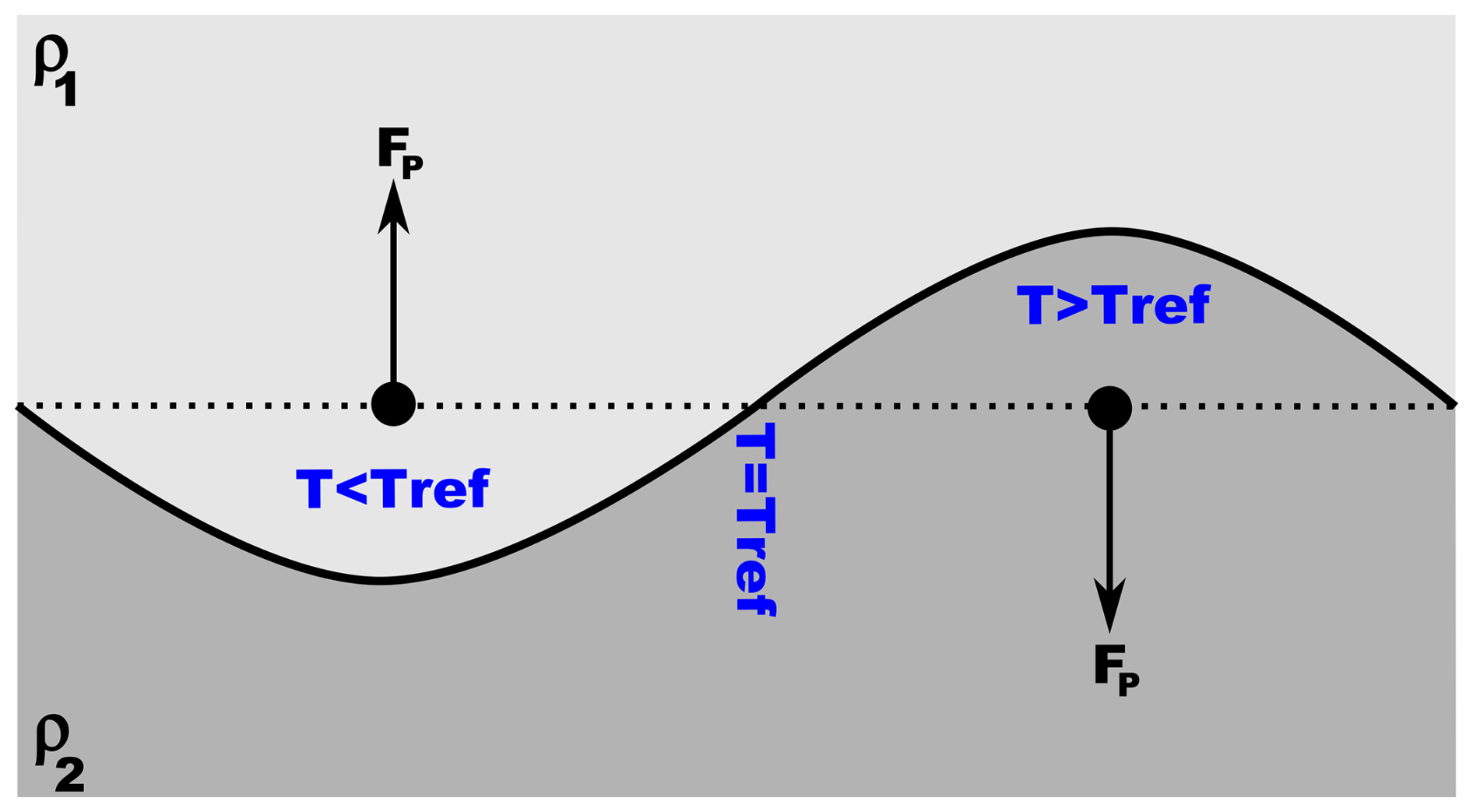
Figure 1 Generation of buoyancy forces (F_P) due to thermally driven topography on the equilibrium depth of a phase transition with a negative Clapeyron slope. Temperatures are given relative to a reference temperature T_ref, defined as the temperature where the phase boundary sits at some reference depth (dotted line). Where $\mathit{\gamma }=\frac{\mathrm{d}P}{\mathrm{d}T}<\mathrm{0}$ and T<T_ref, the equilibrium pressure is greater than that at T_ref, so the phase boundary deepens. Since the less dense upper material (ρ₁) is laterally adjacent to denser material (ρ₂>ρ₁), this produces a positive buoyancy force, opposing the effect of the thermal buoyancy.

Recently, some numerical codes have implemented buoyancy forces using tables of computed thermodynamic properties either directly from differences in density (e.g. Ita and King, 1994; Nakagawa et al., 2009) or by reformulating the governing equations in terms of entropy (e.g. Dannberg et al., 2022; Li et al., 2025), and these forces (assuming spatial gridding in the tables and geodynamic modelling does not “miss” minor reactions) should all be “complete” – capturing the effect in buoyancy forces of the density changes found in these thermodynamic tables, irrespective of how many or of what morphologies these phase transitions have in P–T space. The aim of this work is to consider from a simpler theoretical perspective how large a role these more complicated phase diagram morphologies could play and to inform intuitions about the extent that reactions described by a single Clapeyron slope approximate phase boundaries in Earth materials.

Here, we consider two examples – the post-spinel reactions via akimotoite and the post-garnet reaction – which represent two basic morphologies beyond the well-understood “linear” phase boundary morphology: “branching” and “curving” morphologies respectively.

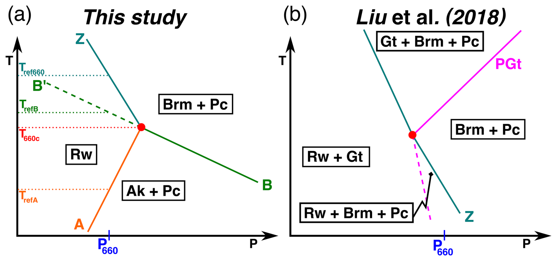
Figure 2 Sketch diagrams of branching phase diagram morphologies as implemented in geodynamic simulations. Temperature and pressure ranges are different between panes – the pressure at 660 km depth (P₆₆₀) is included for reference. (a) Sketch phase diagram of olivine system in the 660 phase boundary region. The reference temperature for reactions A (orange line) and B (green line) is calculated by projecting out from the triple point, described by temperature T_660c – for reaction B this is done along the pseudo-boundary beyond the triple point (dashed line labelled “B^′”). (b) Sketch pyrolite (60 % olivine, 40 % garnet) phase diagram implemented by Liu et al. (2018) at the intersection of the post-spinel reaction (blue line labelled according to our convention as Z) and the post-garnet reaction (magenta line labelled as “PGt”). Note that the PGt implemented by Liu et al. (2018) in their geodynamic simulations is much shallower than the post-garnet reaction we consider below since they are motivated by a different set of data (Hirose, 2002). Liu et al. (2018) do not consider the role of the post-garnet reaction at temperatures beneath the intersection – the dashed magenta line here represents this neglected necessary phase boundary.

1.1 Branching phase boundaries: post-spinel reactions via akimotoite

At cooler temperatures, bridgmanite in the post-spinel reaction ($\text{Rw}\to \text{Brm}+\text{Pc}$, hereafter reaction “Z”) is replaced by the ilmenite group mineral akimotoite (e.g. Yu et al., 2011) – $\text{Rw}\to \text{Ak (akimotoite)}+\text{Pc}$ (hereafter reaction “A”) followed by transformation of Ak→Brm (hereafter reaction “B”) (see Fig. 2a). Recently, there has been interest in the potential geodynamic role of reaction B, whose Clapeyron slope is also negative but significantly larger in magnitude than that of the global reaction Z, and so mineral physicists and seismologists have suggested that reaction B might potentially provide a mechanism to aid the stagnation of slabs (e.g. Cottaar and Deuss, 2016; Chanyshev et al., 2022).

This is not the first contribution to the geodynamic literature that considers the effect of a branching phase boundary morphology on mid-mantle dynamics. Using a phase function (after Christensen and Yuen, 1985), Liu et al. (2018) considered the effect of a sharp post-spinel reaction and broad linear post-garnet reaction interacting on a plume, forming a similar branched morphology except flipped in temperature (i.e. the “trunk” is on the cooler side, and the “branches” are on the warmer side of the critical temperature – see Fig. 2b). The phase diagram used by Liu et al. (2018) does not conserve entropy and volume changes around the phase boundary intersection since beneath the intersection temperature they should still have a garnet-out reaction, which they neglect to include. However, taking their implemented phase boundary buoyancy forces as is, they show that the post-garnet reaction with a positive Clapeyron slope has a strong impact on the local phase boundary topography and significantly reduces the counter-convective effect of the post-spinel reaction on the long-length-scale velocity field (Liu et al., 2018).

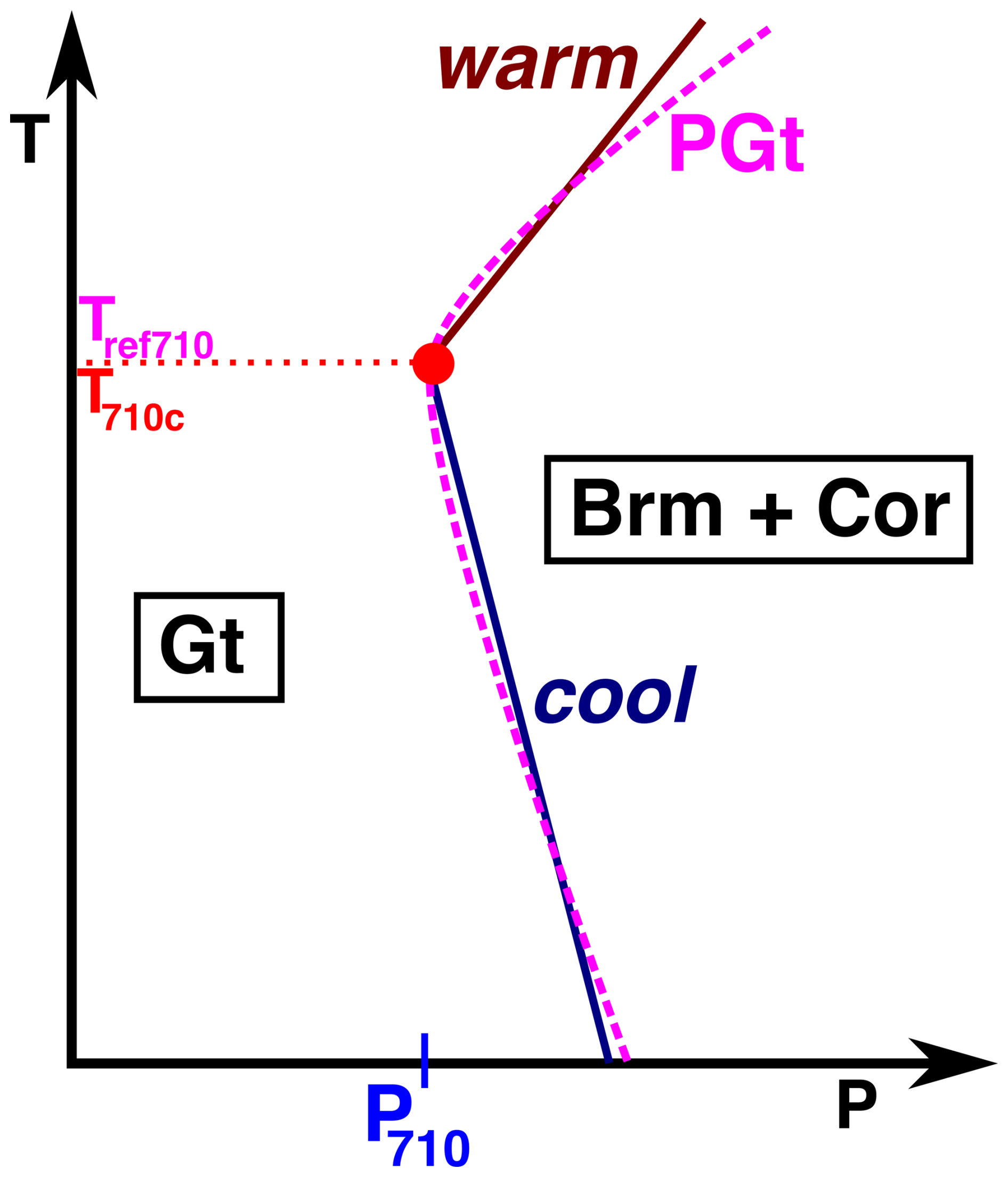
Figure 3 Sketch phase diagram of post-garnet reaction with temperature-dependent phase boundary. Smooth dashed magenta curve shows the phase boundary fitted by Ishii et al. (2023), and straight navy and maroon lines sketch the implementation strategy here of treating the curved phase boundary as two straight boundaries meeting at a critical temperature. Pressure at 710 km depth (P₇₁₀) where the sheet mass anomaly is implemented is indicated. Phases Ishii et al. (2023) found to be stable indicated – Cor: corundum.

1.2 Curving phase boundaries: post-garnet reaction with variable Clapeyron slopes

Recently, Ishii et al. (2023) suggested that due to the temperature-dependent heat capacity of garnet at lower mantle pressures, the post-garnet reaction would have a negative Clapeyron slope at cooler temperatures and a positive Clapeyron slope at warmer temperatures (see Fig. 3). Additionally, Ishii et al. (2023) suggest that due to the presence of a small amount of stishovite, the post-garnet reaction is narrow instead of a broad, divariant reaction, as has generally been assumed. Ishii et al. (2023) suggest that their temperature-dependent Clapeyron slope is responsible for slab stagnation whilst permitting plumes to pass unimpeded through the lowermost mantle transition zone. We describe this phase boundary morphology as a curving morphology. A strongly curved post-spinel transition has also recently been suggested (Dong et al., 2025). Here we consider the effects of a curved post-garnet transition on dynamics, but the intuitions gained with post-garnet can also be transferred to the effects of post-spinel.

1.3 This contribution

In this contribution we illustrate the potential effects of these phase boundary morphologies. In Sect. 2 we describe the implementation of phase boundary topography buoyancy forces in TERRA and how we modify the current implementation for a curving and branching morphology and show the impact of these forces in simple thermal convection models to build intuitions about the controls and limitations of their impacts on flow. In Sect. 3 we illustrate the (non-)impact of the curving morphology on a mantle with a more Earth-like model setup. As we are considering the impact of these diverse phase transitions on convection, we do not consider the role of some other factors such as radial viscosity structure (e.g. Garel et al., 2014; Cerpa et al., 2022), the temperature dependence of rheology (King and Ita, 1995), or the kinetics of phase transformations (King et al., 2015), which have been suggested and shown in numerical simulations to have an effect on the behaviour of downwellings in the mid-mantle.

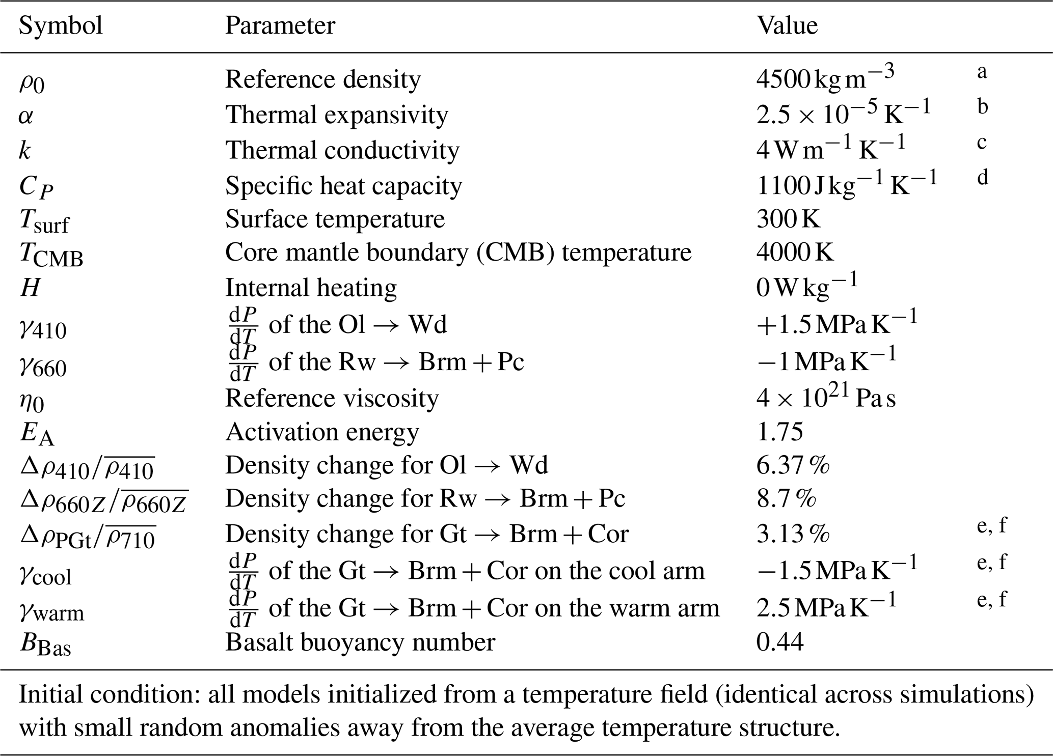
Table 1 Values taken as constant across all convection simulations.

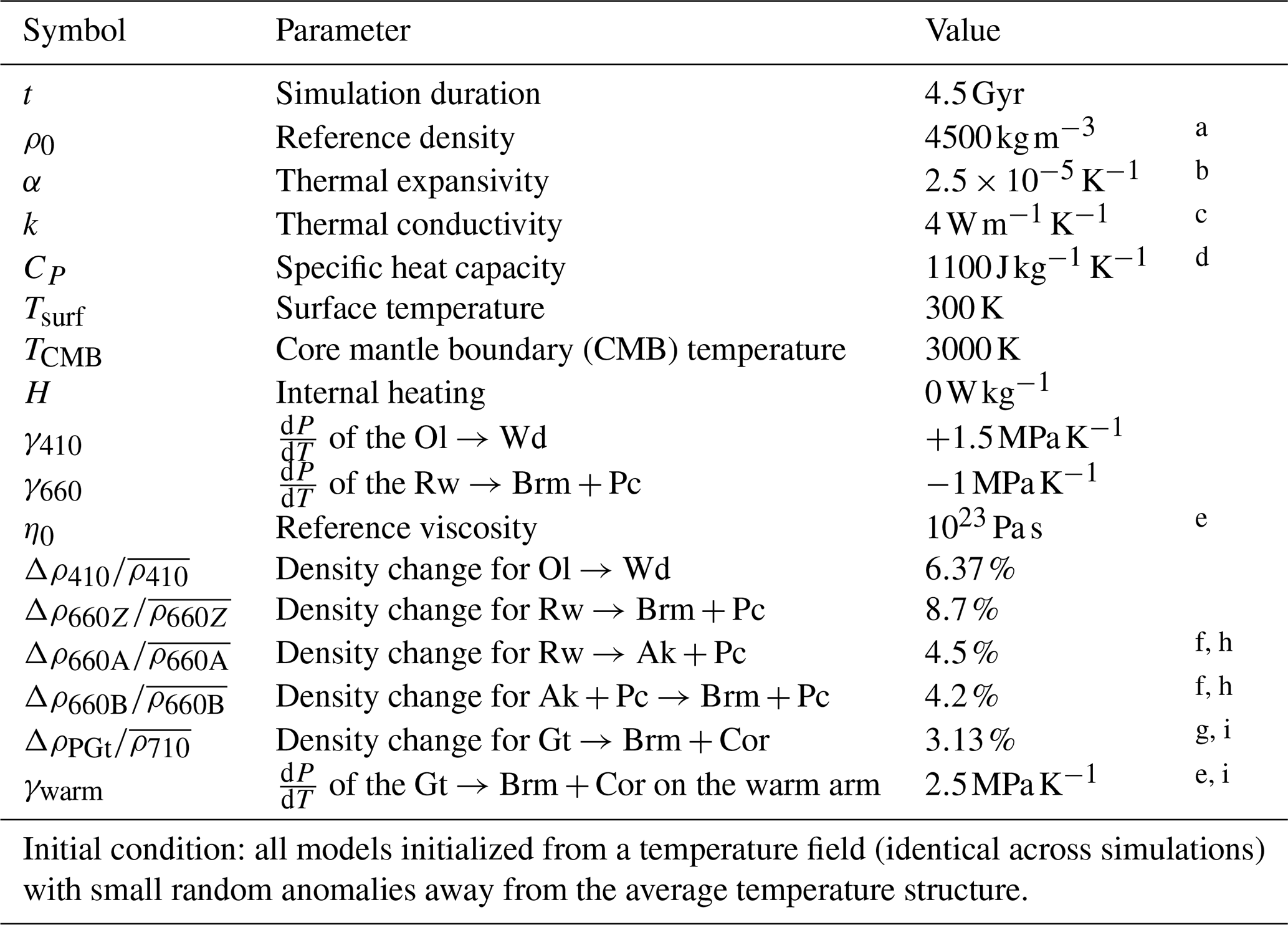
^a Reasonable typical mantle density, e.g. Dziewonski and Anderson (1981).
Values taken from the following: ^b Poirier (p. 61, 2000). ^c Clauser and Huenges (p. 122, 1995). ^d Panton (2020). ^e Deschamps and Cobden (2022). ^f Kojitani et al. (2022). ^g Ishii et al. (2023). ^h For Ak simulation, not included in PGt or reference simulations. ⁱ For PGt simulations, not included in Ak or reference simulations

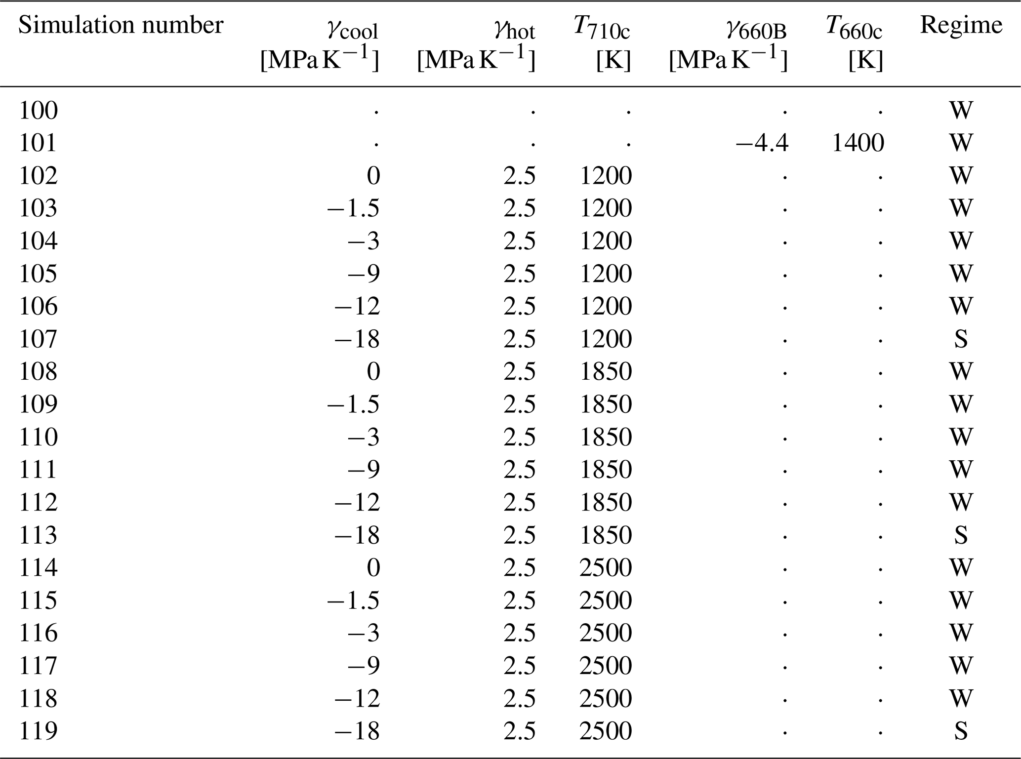
Table 2 Simple thermal convection simulations, varied parameters, and dynamic regimes classified as whole mantle convection (W) or whole mantle convection with downwelling stagnation (S). “⋅” indicates that the parameter is not defined for this simulation as the relevant reaction was not included.

2 Simple thermal convection models

To illustrate the potential dynamics that these diverse phase boundary morphologies can produce, we run simulations using the mantle convection code TERRA (e.g. Baumgardner, 1983; Panton et al., 2022) detailed in Table 2. We consider in turn the implementation of phase boundaries in TERRA, the implementation of branching phase boundaries and their possible effects, and finally the implementation and effects of curving phase boundaries. Here we aim only to illustrate potential dynamic regimes, so our simulations are not particularly Earth-like. We will consider a more sophisticated (but still comparatively simple) pair of simulations in Sect. 3.

2.1 Implementation of phase transitions

We implement all the reactions (post-olivine, post-spinel, and the more complex examples considered below) using the sheet mass anomaly method (e.g. Tackley et al., 1993; Bunge et al., 1997). This more simple method allows a direct consideration of phase boundary transition parameters. In a Boussinesq approximation, the method adds a buoyancy stress (Δσ) due to the topography of the phase transition as

$$\begin{array}{}\text{(3)}& \mathrm{\Delta }\mathit{\sigma }=\mathit{\gamma }\cdot {\displaystyle \frac{\mathrm{\Delta }\mathit{\rho }}{\mathit{\rho }}}\cdot (T-T_{\text{ref}})\end{array}$$

on the nodes at the reference depth of the phase transition. In this expression, T is the temperature at the node and T_ref is the reference temperature (see Fig. 2a) of the phase boundary (temperature where the phase boundary sits at the reference depth (i.e. 410 or 660 km in depth)), Δρ is the density difference associated with the phase change, and γ is the Clapeyron slope of the phase transition.

2.2 Reference model

To compare the effect of including branching and curving morphologies, we first consider a reference model with a linear, post-spinel reaction (Simulation number 100). All the other simple convection models are based on this model setup. The simulations are run in TERRA, using the parameters listed in Table 1. The models are run for 4.5 Gyr (to thermal quasi-steady state; see Fig. A2), and the reference model is visualized in Fig. 5a. In all simulations, as well as the deeper mantle transition zone reactions considered in this paper, we include the olivine-out reaction at 410 km depth. For these simple simulations we use an isoviscous rheology and take the Boussinesq approximation; these are both significant simplifications away from the real Earth but allow us to assess the impact of the phase boundary topography buoyancy forces. In taking the Boussinesq approximation, we do not include the direct effect of the enthalpy of reaction on the temperature field. This latent heat effect is generally smaller than the effect of the phase boundary topography and has the opposite effect on the convection (e.g. Ita and King, 1994; Steinberger, 2007; Dannberg et al., 2022), hence the work here represents an upper bound on the potential effect of the phase transition on the dynamics. Similarly, since a temperature-dependent rheology would tend to stiffen cold downwellings (that are subject to the additional counter-convective forces discussed in this paper), and stiff downwellings have been shown to be less sensitive to stagnation than downwellings in an isoviscous mantle (e.g. Zhong and Gurnis, 1994; King and Ita, 1995), this simplification again leads to an overestimation of the potential effect of these phase boundaries.

We do not include the effect of laterally varying composition on the relative strength of the reactions. Whilst the mantle as a whole has a pyrolytic composition (∼60 % olivine and ∼40 % garnet in the upper mantle, e.g. Bina and Helffrich, 2013), compositional heterogeneities generated by melting at the surface result in regions enriched and depleted in garnet and pyroxene in the upper mantle – in entirely enriched regions (high in basalt) of the mantle, no post-spinel reaction is expected (and the post-garnet reaction – see below – would be at its maximum strength), and in entirely depleted regions of the mantle the post-spinel reaction should be at its maximum strength. We assume that each reaction affects all of the material around it and thus provide an overstated upper bound on the influence of reactions on mantle flow.

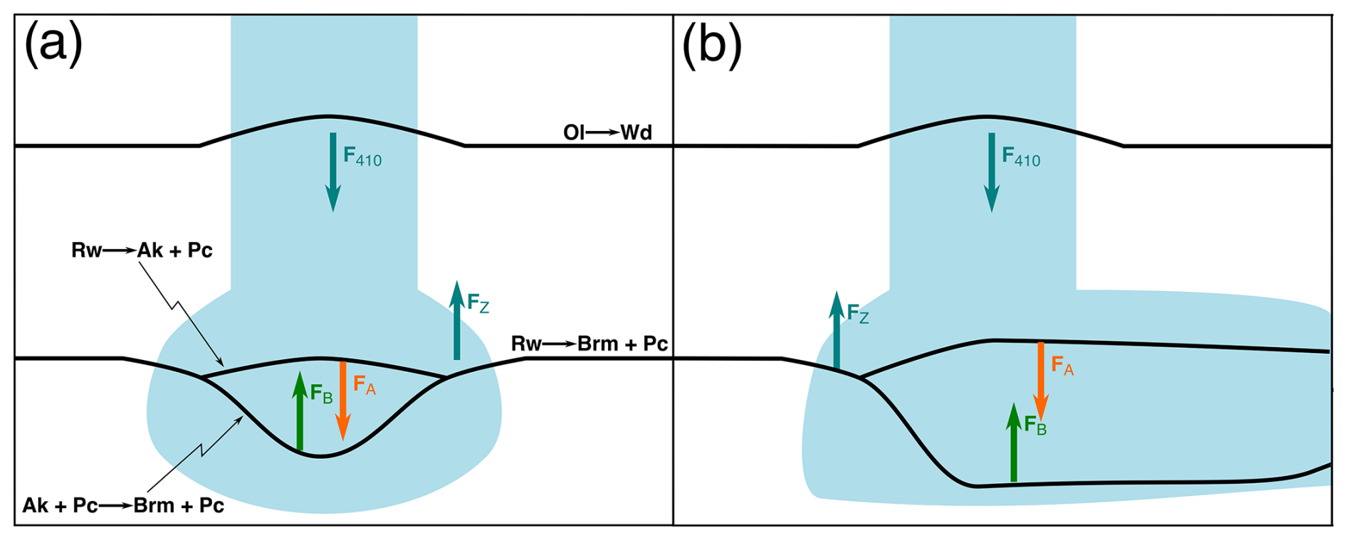
Figure 4 Sketches illustrating the forces due to phase boundary topography of reactions A and B in cool downwellings (F_A and F_B respectively). (a) In a vertical slab, where the split phase transition region is comparatively small, and the opposing phase transition topography buoyancy forces act on near-identical regions. (b) In a stagnating slab, where the phase transitions spread further apart, the forces act on distinct regions. F₄₁₀ denotes the force due to the Ol→Wd reaction, at 410 km depth, and F_Z the force due to the $\text{Rw}\to \text{Brm}+\text{Pc}$ reaction (reaction Z in Fig. 2a).

2.3 Implementing branching phase transitions (post-spinel via akimotoite)

The sheet mass anomaly approximation (Tackley et al., 1993) assumes that the length scale of the topography on the phase boundary is less than or similar to the length scale of the thermal structure that drives the flow. For a downwelling body whose temperature is 500 K below the critical temperature of the reactions A, B, and Z with Clapeyron slopes of ${\mathit{\gamma }}_{\mathrm{A}}=+\mathrm{1.5}$ and ${\mathit{\gamma }}_{\mathrm{B}}=-\mathrm{6}$ MPa K⁻¹ and a mid-mantle radial pressure gradient of 40 MPa km⁻¹, we estimate a maximum separation between the phase transition surfaces inside the downwelling body as on the order of 100 km ($(\mathrm{1.5}+\mathrm{6}[\mathrm{MPa}{\mathrm{K}}^{-\mathrm{1}}\left]\right)\cdot \left(\mathrm{500}\right[\mathrm{K}\left]\right)/\left(\mathrm{40}\right[\mathrm{MPa}{\mathrm{Km}}^{-\mathrm{1}}\left]\right)$). In our global convection models (with a comparatively high mantle viscosity of 10²³ Pa s), our slabs end up much wider than this separation, allowing us to consider the phase transition boundary topography force from both the reactions A and B as acting at similar depths (see Fig. 4). We are probably at the edge of where this approximation is valid (moving toward weaker and temperature-dependent geological mantle rheologies would probably break this simplification for these reactions), but the theoretical understanding developed below suggests significant effects on global dynamics are unlikely. Given that this approximation overstates the dynamic effect branching reactions can have on mantle flows, we expect our conclusions to be robust. Therefore, Eq. (3) becomes

$$\begin{array}{}\text{(4)}& \mathrm{\Delta }{\mathit{\sigma }}_{\mathrm{660}}=\left\{\begin{array}{ll}{\mathit{\gamma }}_{\mathrm{Z}}\cdot \frac{\mathrm{\Delta }{\mathit{\rho }}_{\mathrm{Z}}}{\mathit{\rho }}(T_{\mathrm{660}}-T_{\text{ref}\mathrm{660}})& T_{\mathrm{660}}\ge T_{\mathrm{660}\text{c}}\\ & \\ {\mathit{\gamma }}_{\mathrm{A}}\cdot \frac{\mathrm{\Delta }{\mathit{\rho }}_{\mathrm{A}}}{\mathit{\rho }}\cdot (T_{\mathrm{660}}-T_{\text{refA}})& \\ +{\mathit{\gamma }}_{\mathrm{B}}\cdot \frac{\mathrm{\Delta }{\mathit{\rho }}_{\mathrm{B}}}{\mathit{\rho }}\cdot (T_{\mathrm{660}}-T_{\text{refB}})& T_{\mathrm{660}}<T_{\mathrm{660}\text{c}},\end{array}\right.\end{array}$$

where T_660c is the temperature of the triple point, where reactions A, B, and Z meet (see Fig. 2a).

We do not have free choice over the values of the Clapeyron slopes and density changes at branching intersections, since entropy and volume changes are properties of state alone. The changes in entropy and volume from one state to another must be equal regardless of the path taken. With reference to Fig. 2a, the entropy and volume changes must be the same whether the assemblage changes from Rw to Brm+Pc via reaction Z or via reactions A and B. Assuming ΔV≪V and re-writing Eq. (4) in terms of volume and entropy change we get

$$\begin{array}{}\text{(5)}& \mathrm{\Delta }{\mathit{\sigma }}_{\mathrm{660}}=\left\{\begin{array}{ll}\frac{-\mathrm{\Delta }{S}_Z}{V}\cdot (T_{\mathrm{660}}-T_{\text{ref}})& T_{\mathrm{660}}\ge T_{\mathrm{660}\text{c}}\\ & \\ \frac{(-\mathrm{\Delta }{S}_{\mathrm{A}}-\mathrm{\Delta }{S}_{\mathrm{B}})}{V}\cdot (T_{\mathrm{660}}-T_{\text{ref}})& T_{\mathrm{660}}<T_{\mathrm{660}\text{c}}.\end{array}\right.\end{array}$$

As $\mathrm{\Delta }{S}_{\mathrm{A}}+\mathrm{\Delta }{S}_{\mathrm{B}}=\mathrm{\Delta }{S}_{\mathrm{Z}}$, the temperature dependence of the phase boundary topography buoyancy force has to be the same either side of the triple point if we apply these forces using a sheet mass anomaly approximation.

Yu et al. (2011)Ye et al. (2014)Hernández et al. (2015)Kojitani et al. (2016)Kojitani et al. (2022)Chanyshev et al. (2022)

Table 3 Values for parameters recently calculated by mineral physicists. “⋅” indicates that this value is not evaluated in the publication.

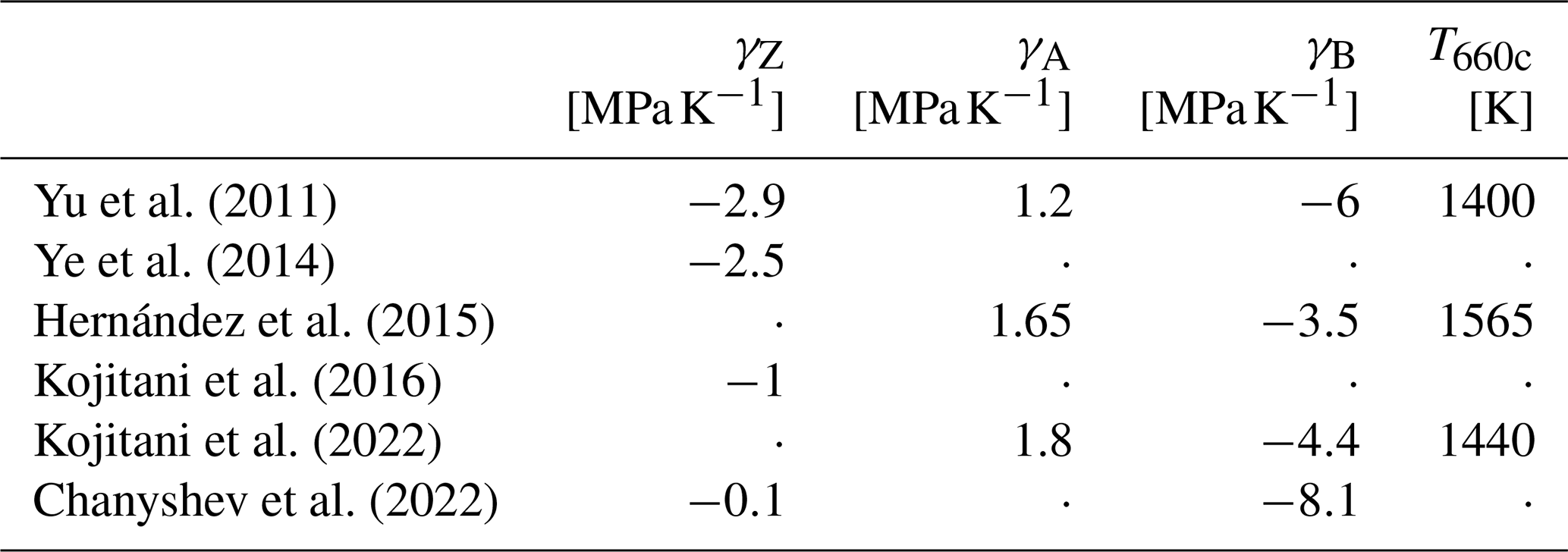
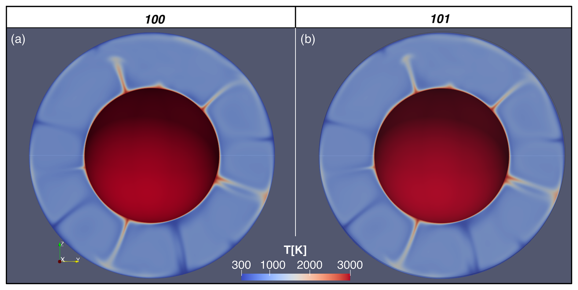
Figure 5 Visualization of convection simulations after 4.5 Gyr of evolution (a) Reference case (Simulation number 100) – post-olivine and post-spinel reactions included, but no other reactions are included. (b) Branching case (Simulation number 101) – akimotoite reactions implemented using values suggested by Kojitani et al. (2016, 2022). Note that there is no significant difference between the thermal structure of the simulations, as expected.

2.4 Results for thermodynamically consistent branching phase transitions

In order to demonstrate the (non-)effect of implementing a thermodynamically consistent branched morphology using the implementation described above, a simulation based on the reference case was run but with ${\mathit{\gamma }}_{\mathrm{A}}=\mathrm{1.8}\mathrm{MPa}{\mathrm{K}}^{-\mathrm{1}}$ and ${\mathit{\gamma }}_{\mathrm{B}}=-\mathrm{4.4}\mathrm{MPa}{\mathrm{K}}^{-\mathrm{1}}$ (i.e. the values of Kojitani et al., 2016, 2022, but these are similar to other published values for the Clapeyron slopes – see Table 3). This is visualized after 4.5 Gyr in Fig. 5b, where it is obvious that the simulations are very nearly identical, highlighting that the combined phase boundary buoyancy forces of reactions A and B result in an extremely similar resultant force to what reaction Z would have produced. We further verify this in Fig. A1, where we compare the radial temperature histograms for the two simulations – demonstrating again that they are nearly identical.

2.5 Implementing curving phase transitions (post-garnet)

As illustrated in Fig. 3, the curving post-garnet reaction is here implemented using two straight lines to approximate the parabolic form suggested by Ishii et al. (2023). Since the phase boundary topography implied by Ishii et al. (2023) is relatively modest, the sheet mass anomaly approximation in TERRA is suitable for application to this reaction. We calculate the buoyancy stresses at 710 km depth due to this topography as

$$\begin{array}{}\text{(6)}& \mathrm{\Delta }{\mathit{\sigma }}_{\mathrm{710}}=\left\{\begin{array}{ll}{\mathit{\gamma }}_{\text{warm}}\cdot \frac{\mathrm{\Delta }{\mathit{\rho }}_{\text{PGt}}}{\mathit{\rho }}(T_{\mathrm{710}}-T_{\text{ref}\mathrm{710}})& T\ge T_{\mathrm{710}\text{c}}\\ & \\ {\mathit{\gamma }}_{\text{cool}}\cdot \frac{\mathrm{\Delta }{\mathit{\rho }}_{\text{PGt}}}{\mathit{\rho }}\cdot (T_{\mathrm{710}}-T_{\text{ref}\mathrm{710}})& T<T_{\mathrm{710}\text{c}},\end{array}\right.\end{array}$$

where γ_warm and γ_cool are the Clapeyron slopes above and below the critical temperature. By choosing the depth at which the post-garnet phase boundary force is implemented as 710 km (the minimum depth of the phase boundary found by Ishii et al., 2023), this means that a single reference temperature T_ref710 describes both the warm and cool legs of the “curved” reaction and is also the temperature at which the Clapeyron slope of the reaction changes T_710c. To explore the role that this curving reaction can have, we vary two parameters explicitly – T_710c and γ_cool in the ranges of 1200 to 2500 K and 0 to $-\mathrm{18}\mathrm{MPa}{\mathrm{K}}^{-\mathrm{1}}$ respectively over 18 simulations (see Table 2).

2.6 Results for curving (post-garnet) phase transition

Select simulations with a post-garnet inspired curving phase change are visualized in Fig. 6. At the highest magnitude of γ_cool considered here ($-\mathrm{18}\mathrm{MPa}{\mathrm{K}}^{-\mathrm{1}}$) (Fig. 6a) many downwellings fail to enter the lower mantle. Decreasing the value of γ_cool (compare results in Fig. 6c) results in a mode of convection similar to that seen for the reference case (see Fig. 5a).

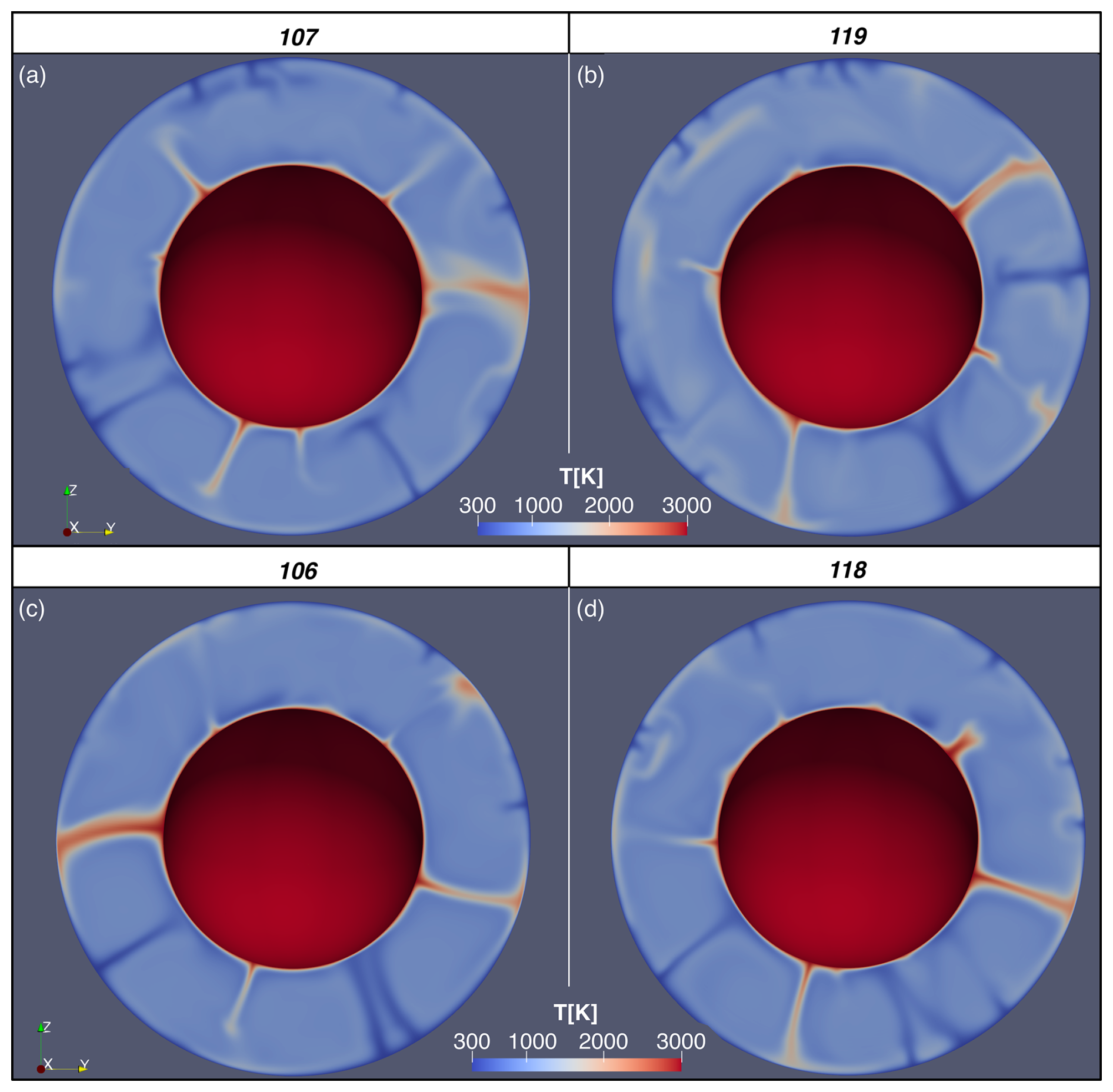
Figure 6 A great circle slice through the temperature field of 3D of convection simulations with PGt reaction present after 4.5 Gyr. (a, b) Where ${\mathit{\gamma }}_{\text{cool}}=-\mathrm{18}\mathrm{MPa}{\mathrm{K}}^{-\mathrm{1}}$ after 4.5 Gyr of evolution. (a) Simulation number 107, T_710c=1200 K. (b) Simulation number 119, T_710c=2500 K. (c, d) Where ${\mathit{\gamma }}_{\text{cool}}=-\mathrm{12}\mathrm{MPa}{\mathrm{K}}^{-\mathrm{1}}$ after 4.5 Gyr of evolution. (c) Simulation number 106, T_710c=1200 K. (d) Simulation number 118, T_710c=2500 K.

2.6.1 Effect of T_710c

As well as the magnitude and sign of the Clapeyron slope, another important parameter in determining the vigour of convection is T_710c – which controls the portions of the mantle affected by pro- and contra-convective forcings from the phase boundary topography, with higher values of T_710c meaning that more of the downwellings are affected by the cool arm of the PGt reaction. With an increasing proportion of the Earth's mantle subject to a counter-convective forcing in cold downwellings in Fig. 6b, stagnation becomes more likely. Considering Fig. 6a and b, where the simulations have a higher magnitude of γ_cool (−18 vs. $-\mathrm{12}\mathrm{MPa}{\mathrm{K}}^{-\mathrm{1}}$) than in Fig. 6c and d – we again see more downwellings stagnating in the right-hand panel and large volumes of cold material building up in the mid-mantle (e.g. stagnation at ∼ “8 o'clock” in Fig. 6b). In Fig. 6a, by comparison, cold material is able to start entering the lower mantle with less negative thermal buoyancy (e.g. the downwelling at “9 o'clock” descending with a bulge of stagnated material in the mid-mantle, or at “11 o'clock” a pile of cold material in the mantle transition zone (MTZ) starting to descend into the lower mantle). This illustrates that increasing the value of T_710c, whilst not exerting a large enough influence to change the mode of convection here, is changing the magnitude of the local counter-convective effect on the downwellings. Considering the relative mass flux at 720 km depth (see Fig. A3), we see that Simulation 107 has a much higher mass flux than the other cases that showed downwelling stagnation, suggesting that at even lower T_710c, we might expect whole mantle convection even at extremely negative values of γ_cool.

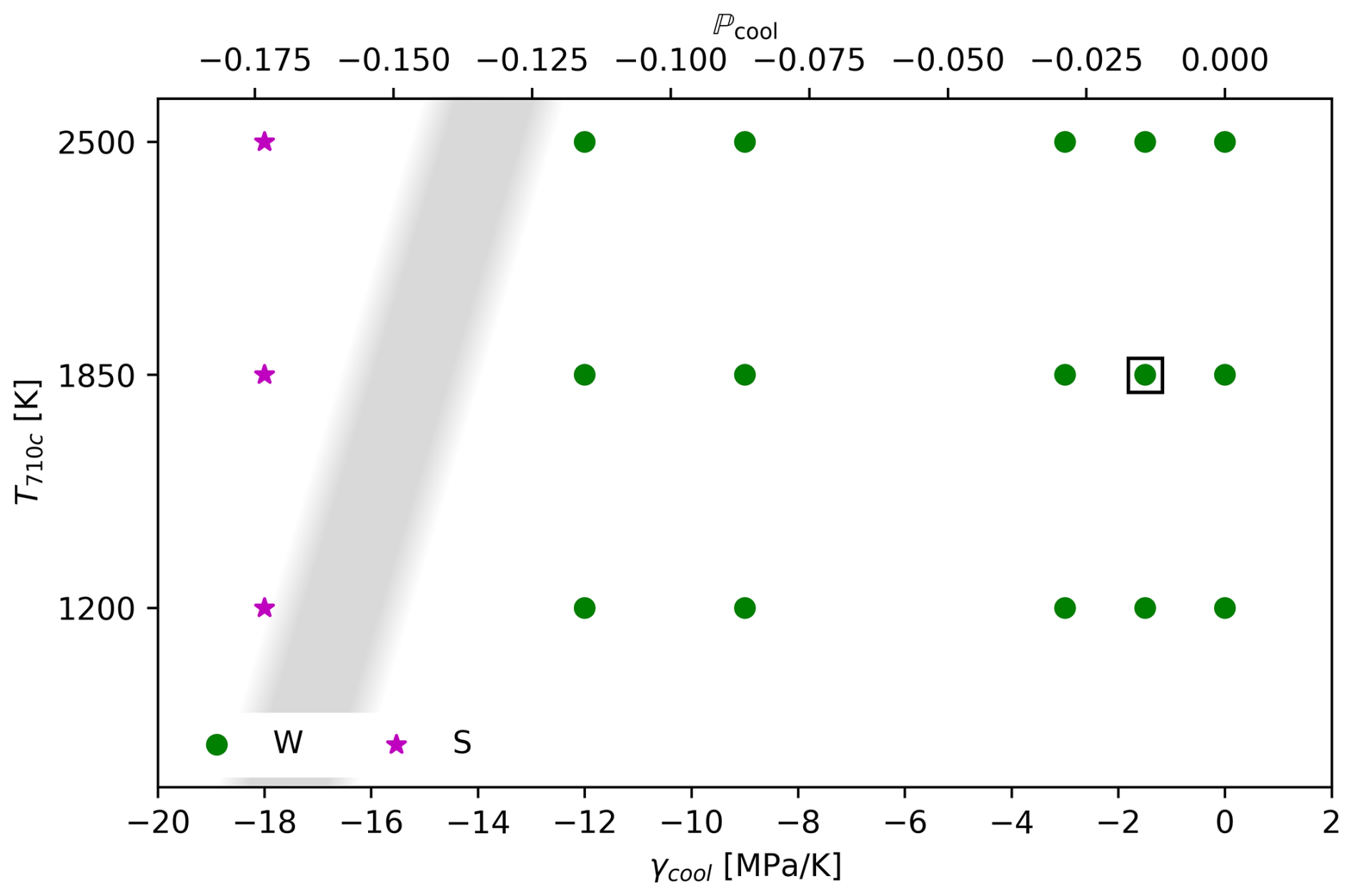
Figure 7 Regime diagram of model runs plotted on their values of T_710c and γ_cool. Simulations in the mode of whole mantle convection and in a mode with slab stagnation are marked W and S respectively. The approximate region and inferred slope polarity of the boundary between these regimes is indicated by the grey shading. Simulation 109, which takes the values proposed by Ishii et al. (2023) for γ_cool and T_710c, is highlighted by a black square.

2.6.2 Dynamic regimes

We categorize our 18 simulations into two groups based on the presence or absence of stagnant cold material in the mid-mantle: “whole mantle convection” (“W”) and “whole mantle convection with downwelling stagnation” (“S”). Simulations that we categorize as S have lower surface heat fluxes when they reach quasi-steady state than those in regime W (compare magenta and green lines in Fig. A2). The simulations with stagnating slabs and higher values of T_710c (Simulation numbers 113 and 119) have lower heat fluxes at 4.5 Gyr than the simulation with a lower value of T_710c (Simulation number 107 although this varies over the simulation duration). A regime diagram of these models plotted with their values of T_710c and γ_cool is shown in Fig. 7. Note that there is no change of regime until much higher magnitude values of γ_cool than those suggested by Ishii et al. (2023) to apply for the actual post-garnet reaction in the Earth. As illustrated in Fig. 6, there is some variation in downwelling behaviour within these regimes, but T_710c plays a secondary role to γ_cool. In Fig. 7 we include a sketched boundary between the two regimes; the slope of this line is inferred to be positive since there is more stagnation in Simulation 119 than Simulation 107 – but with this suite of simulations the exact position of the regime boundary is difficult to constrain. We emphasize that this change in dynamic regime does not occur until a much more negative phase parameter than suggested by current data for the garnet-out reaction (Ishii et al., 2023).

As well as considering the morphology of the downwellings (as in Fig. 6), we also consider the effect of the phase transition on the flow of material through the mid-mantles of our simulations. In Fig. A3b we plot the root mean square (rms) of the radial component of velocity as a function of depth for each of the simulated mantles. Simulations 119 and 113 have lower radial velocities in a broad region of their mid-mantles compared to the simulations undergoing whole mantle convection (e.g. Simulation 100). Simulation 107, which we classified as being in regime S by inspection of its thermal structure, has slightly lower radial velocities than the W cases. We also present (Fig. A3a) the ratio of mass flux at 720 km depth and the maximum mass flux during the evolution of the simulated mantles. Again, after the first mantle overturn, Simulations 119 and 113 have a much weaker mass flux than the simulations in the whole mantle convection regime. The relative mass flux in these simulations increases during the model evolution, with major upswings in mass flux, with percent-of-maximum mass flux variations on 100 Myr timescales. Simulation 107 has a higher mass flux than the other S cases, but its flux is still a step lower than the mass flux of the W regime simulations and evolves in a fashion distinct from those simulations. This likely represents that in simulation 107 there is regional ponding on some downwellings (around 12 o'clock, Fig. 6a), whereas others descend directly (4 o'clock) strongly enough that there is sufficient downwelling to permit upwellings to rise unimpeded, unlike in 119 (Fig. 6b) where there is some ponding of material in the mid-mantle (9 o'clock).

2.7 Discussion on simple thermal convection models

Using these simple mantle convection models, we have been able to demonstrate the non-effect of a branching reaction (Fig. 5) morphology of ringwoodite out via akimotoite and to demonstrate some of the behaviours possible for a curving phase boundary (Fig. 6). By varying T_710c and γ_cool, we have illustrated that the cold arm of the post-garnet reaction does not change the mode of global convection significantly until γ_cool is an order of magnitude greater than that suggested from the experiments of Ishii et al. (2023). Similar to Bina and Liu (1995), we also found a dependence in convective style on the temperature where the Clapeyron slope changes but found that γ_cool had a much larger impact in our simulations than T_710c. Given that multiple factors about the setup of these simulations favour these phase boundaries being able to have a large effect on the mode of convection, this suggests that in the real Earth, this phase boundary morphology is unlikely to be responsible for the stagnation of slabs.

3 Thermochemical mantle circulation models at Earth-like vigour

The simple mantle convection models of the previous section are non-Earth-like in several respects. Firstly, we have assumed that there is no radiogenic or shear heating and that the models are incompressible – meaning that the mid-mantles in our simulations end up being much cooler on average (∼950 K) than the real Earth's mantle (e.g. ∼1650 K (Waszek et al., 2021)). Further, the convection simulations were isoviscous with a high reference viscosity, so did not represent the temperature and depth dependence of viscosity, which can influence downwellings at the base of the MTZ (e.g. Garel et al., 2014). Together, these result in a Rayleigh number of ∼10⁵ compared to the Earth's value of ∼10⁷ – which may understate the contra-convective effect since global phase transitions have a greater effect at higher Rayleigh number (e.g. Tackley et al., 1993; Wolstencroft and Davies, 2011). In the following sections we describe two significantly more sophisticated mantle circulation models (MCMs) incorporating (“TC1”) and excluding (“TC0”) the effect of the post-garnet reaction.

3.1 Method

Our more Earth-like simulations are also run in TERRA, but instead of a free-slip surface, the surface motion is imposed using the plate motion history of Müller et al. (2022). These plate motions are scaled by a factor of 0.5 (that is, the plate motions are slowed down to mantle velocities) so that the rms surface motions match those produced by the simulated mantle in convection (found during model initialization; see below).

The model rheology is also more Earth-like than the previous simulations, with a reference viscosity closer to the upper mantle viscosity (see Table 4). Viscosity varies according to

$$\begin{array}{}\text{(7)}& \mathit{\eta }={\mathit{\eta }}_{\mathrm{0}}\cdot f_{\mathrm{r}}\cdot e^{-E_{\mathrm{A}}\cdot T^{\prime }},\end{array}$$

where η is the local bulk viscosity, η₀ is the reference viscosity, f_r is the radial viscosity factor (see Fig. 8), E_A is the activation energy, and T^′ is the non-dimensionalized temperature given by $T^{\prime }=\mathrm{0.5}-\frac{T-T_{\text{CMB}}}{T_{\text{surf}}-T_{\text{CMB}}}$. Whilst this rheology law introduces a depth and temperature dependence that we did not have in our simpler convection simulations above, the temperature dependence is less pronounced than that used in other studies (e.g. King, 2009; Javaheri et al., 2024). As discussed in relation to the simple convection simulations above, underestimating the stiffening of cold slabs likely leads to us overestimating the effect the curved phase transition has on the dynamics.

Table 4 Values taken as constant across the mantle circulation simulations.

^a Reasonable typical mantle density, e.g. Dziewonski and Anderson (1981).
Values taken from the following: ^b  Poirier (p. 61, 2000). ^c Clauser and Huenges (p. 122, 1995). ^d Panton (2020). ^e Ishii et al. (2023). ^f for TC1, not included in TC0

Composition is tracked on particles using the method of Stegman (2003). We model melting in the upper parts of the mantle, generating enriched (basaltic) material at the surface, and depleted (harzburgitic) material in the source regions (van Heck et al., 2016). Variations in enrichment affect the intrinsic density – through most of the mantle this means that basalt is ∼2 % denser than lherzolite (“ambient mantle”), but between 660 and 740 km depth, basalt is 5 % less dense than lherzolite as the post-garnet reaction is deeper than the post-spinel, and basalt is enriched in garnet compared to lherzolite and harzburgite (e.g. Yan et al., 2020). Aside from this “basalt density filter” effect (which does not result in a strong concentration of basalt in the deeper parts of the mantle transition zone in these simulations), we do not implement a compositional effect on the phase boundary buoyancy forces.

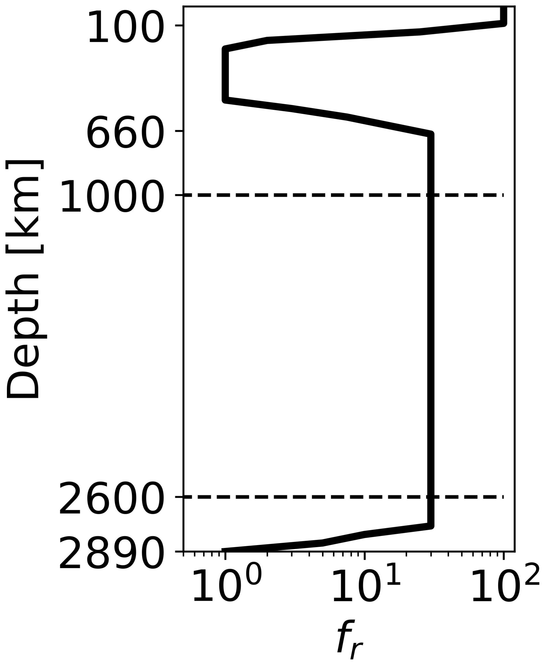
Figure 8 Radial viscosity factor (f_r) variation with depth. Note sharp steps in viscosity at the base of the lithosphere and upper mantle, as well as at the CMB. This radial viscosity structure is chosen to capture key features of the Earth's radial viscosity structure, including a viscosity jump in the mid-mantle.

3.1.1 Model initialization

These simulations undergo a two-stage initialization process. First, a convection simulation (with free slip on both boundaries) is run for 2 Gyr with no active chemistry and without the post-garnet phase boundary forces implemented. The purpose of this stage is to generate a quasi-steady-state thermal structure. In the second stage of initialization, initial velocities of the Müller et al. (2022) plate motion history are used for 400 Myr, particles are initiated, melting is turned on, and the post-garnet phase boundary buoyancy forces are implemented into the simulation for TC1. This stage allows mantle structures to develop in response to the imposed surface motions and also allows the effect of the additional phase boundary buoyancy force to come into effect. Unrealistic flows and related effects arising from the onset of tectonic and igneous processes are allowed to dissipate by the time the main simulation starts. The main simulation is then started with evolving scaled surface velocities imposed as described above.

3.1.2 Choice of parameters for this comparison

We have chosen model parameters (see Table 4) to demonstrate the maximum plausible geodynamic effect of a sharp, curved post-garnet reaction with the parameters suggested by Ishii et al. (2023). To do this we continue to assume that the phase transitions affect all the mantle material at a node and use a comparatively high T_CMB of 4000 K to promote vigorous convection, a state in which counter-convective phase boundary topography forces are more impactful (e.g. Wolstencroft and Davies, 2011).

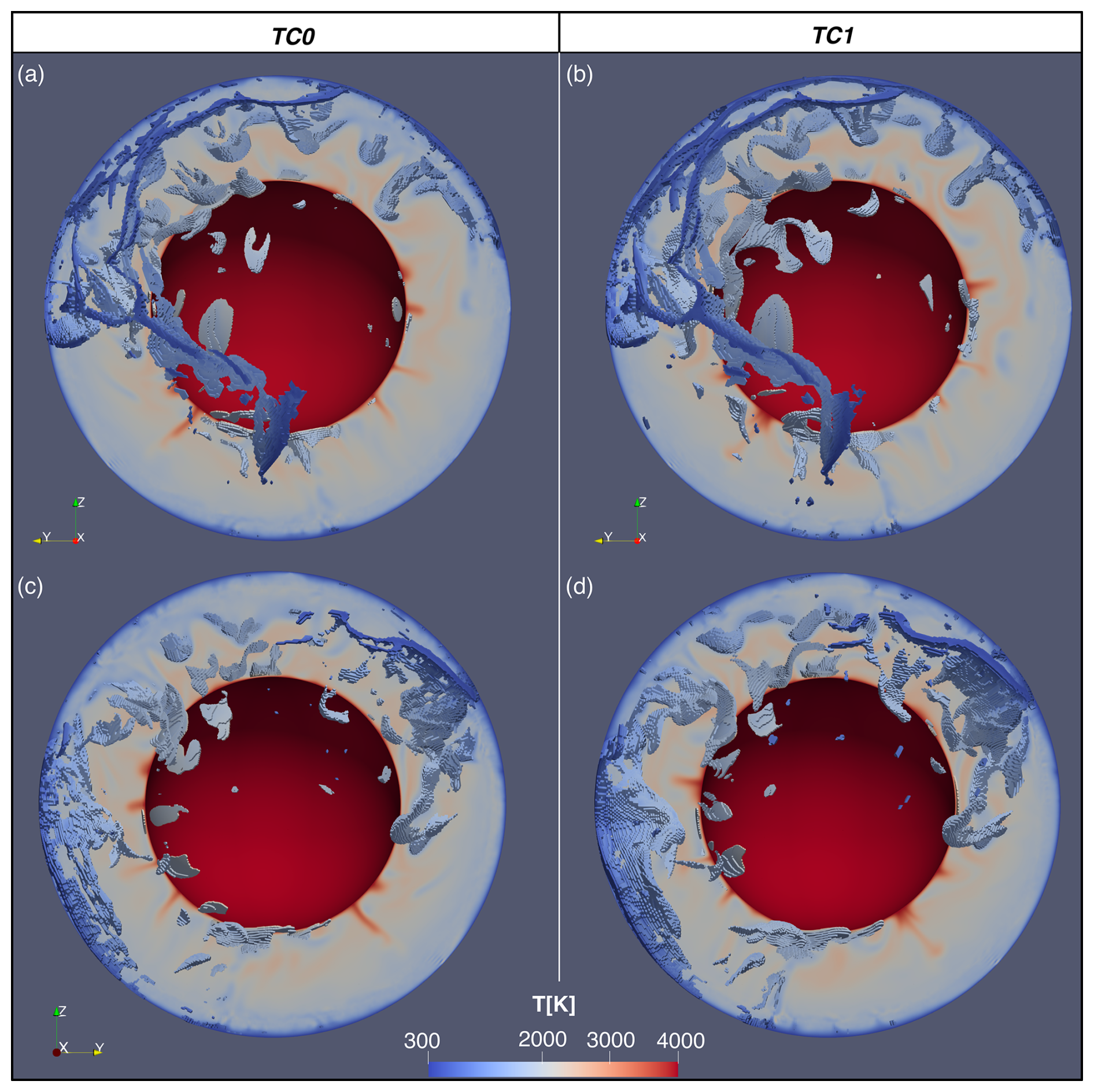
Figure 9 Comparison between reference MCM (TC0, a, c) and MCM with curved PGt phase transition morphology (TC1, b, d). Temperature visualized on latitudinal slice through 90°, as well as on “voxels” beneath 500 K below the radial average temperature. Panels (a) and (b) show the Western Hemisphere, and panels (c) and (d) show the Eastern Hemisphere. Composition visualized in Fig. A4.

3.2 Results

The thermal and composition fields for the reference simulation (“TC0”) and the MCM with the curved post-garnet phase boundary morphology (“TC1”) are visualized in Figs. 9 and A4. In both simulations, cold slabs descend into the lower mantle, carrying enriched and depleted material to the CMB. Some slabs descend directly, while others stagnate in the mid-mantle (e.g. the slabs beneath the north-west Pacific Fig. 9a and b about 1 or 2 o'clock).

3.3 Discussion of thermochemical simulations

Simulations TC0 and TC1 appear to operate in a similar convectional regime and with comparable kinematics (Fig. 9). There are differences between the two simulations – for example, the coldest regions associated with the Nazca slab (Fig. 9c and d, 7–10 o'clock) appear more continuous in the simulation with PGt – however, the introduction of the novel phase boundary topography forces does not cause global slab stagnation or create significant changes in regional slab stagnation. This suggests that while the new forces do have an effect on mantle processes, the effect is small and does not change the mode of mantle circulation.

The radial temperature histograms of the reference case, TC0, and simulation with the curved post-garnet transition, TC1, are extremely similar (Fig. 10), suggestive of a near-identical thermal evolution. In our previous convection simulations, models with large-scale slab stagnation had a distinct thermal evolution (Fig. A2). When we look at the extreme nodes (the 10² and 10¹ number of grid points (NGP) contours), we do see minor differences – for example, the coldest temperatures in Model TC1 are colder at most depths than for the reference model. These minor differences highlight that while there are buoyancy forces associated with a curved post-garnet reaction, they do not significantly change the kinematics or thermal structure of the model.

Whilst the viscosity law of these circulation models is not as strongly temperature-dependent as is likely the case in the Earth, this means that our downwellings are not as viscous as they might otherwise be – rendering them more vulnerable to stagnation than downwellings in the actual Earth (King and Ita, 1995). This supports our extension of this conclusion about the non-impact of the phase boundary morphology from these simplified geodynamic simulations to the Earth's mantle dynamics.

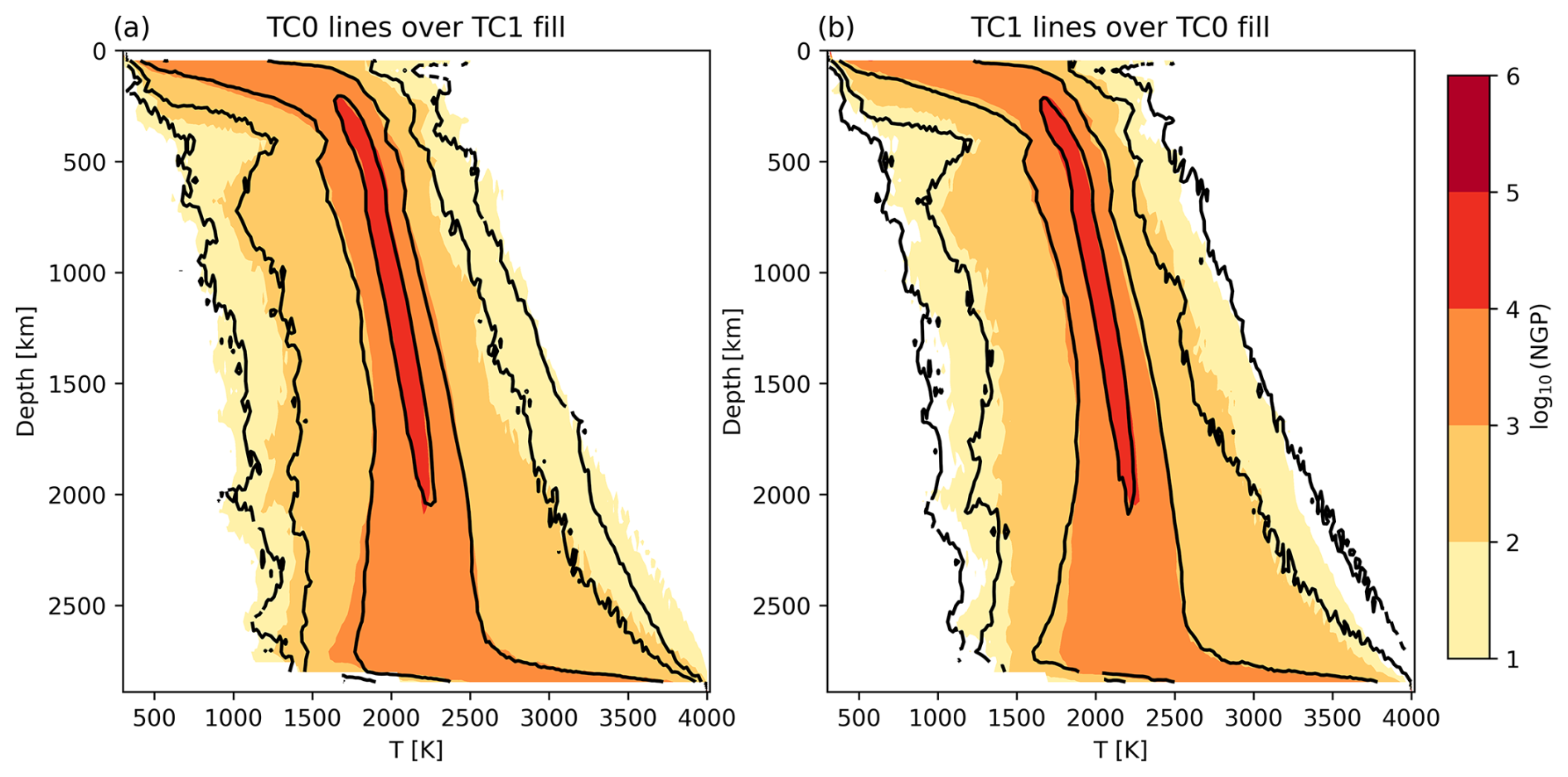
Figure 10 Radial temperature histograms coloured by number of grid points (“NGP”) for PGt simulation TC1 and reference simulation TC0 with contours of the reference (TC0) and PGt (TC1) simulations' radial temperature histograms overlaid respectively (a, b).

4 Discussion

4.1 Branching phase boundaries: thermodynamically possible phase diagrams prohibit additional effects of post-spinel via akimotoite versus direct post-spinel

We have demonstrated above (Eq. 5) that under the sheet mass anomaly approximation, the phase boundary buoyancy forces for two branches must sum to the force of the trunk reaction and have shown that under this condition, no effect on mantle dynamics is observed (see Fig. 5). This is potentially contrary to some of the suggestions in the mineral physics and seismology literature (e.g. Cottaar and Deuss, 2016; Chanyshev et al., 2022). Of course this prohibition only applies strictly where reactions A and B are close enough spatially that the forces can be treated as acting on the same region. As A and B move further apart a distinct counter-convective effect of reaction B could emerge in extremely localized regions of slabs – these regions would be largest in slabs that are horizontal in the lowermost MTZ. Since these regions of slabs would sit within a downwelling exerting a viscous downwards drag and still relatively close beneath reaction A encouraging the descent of material on to them, for reported values of T_660c, γ_A, and γ_B it is difficult to envisage there being much of a dynamic effect in the Earth's mantle.

4.2 Curving phase boundaries: phase buoyancy parameter (ℙ) implied by mineral physics too small to effect global dynamics

In our simple convection simulations, we were able to produce downwellings that stalled in the mid-mantle whilst upwellings rose unimpeded through the post-garnet transition at values of γ_710cool much greater than those suggested for PGt. Furthermore, in a simulation with realistic surface motions and a curved phase boundary with parameters similar to those suggested for the post-garnet reaction by Ishii et al. (2023) we observed no additional slab stagnation compared to a simulation without the curved phase boundary. This result is expected, as the phase buoyancy parameter (using the parameters in Table 4) for the cool post-garnet is −0.014 – much less than that which would be expected to induce a layered or transitional dynamic regime. This is a much smaller magnitude than the value of −0.10 found by Ishii et al. (2023), possibly due to them assuming the thickness of the convecting layer is the above the phase boundary, whereas we assume it is the full depth of the mantle. This is the choice used elsewhere in the geodynamic literature (e.g. Tackley et al., 1994; Bunge et al., 1997; Wolstencroft and Davies, 2011), since this is the thickness of the layer that would convect without the presence of an extremely counter-convective phase transition.

It is worth considering how well current theoretical models of a global linear reactions align with the temperature-restricted reactions considered in our simulations.

For example, at a Rayleigh number of 1.4×10⁵ (the same as in our simulations from Sect. 2), Wolstencroft and Davies (2011) predicted regime changes from whole mantle convection to “transitional” convection at $\mathbb{P}<-\mathrm{0.25}$ and to layered convection at $\mathbb{P}<-\mathrm{0.32}$. These thresholds are considerably more negative than the value of $\mathbb{P}\sim -\mathrm{0.175}$ at which we see a regime change (see Fig. 7). This discrepancy may be explained by the temperature restriction, which could truncate cold thermal structures, making them more vulnerable to downwelling stagnation (Tackley et al., 1993). Wolstencroft and Davies (2011) assume their regime boundaries follow the form $\mathbb{P}=\mathit{\alpha }{\mathit{Ra}}^{-\mathit{\beta }}$, where α and β are constants. As the Rayleigh number increases, the slopes of these curves tend to flatten. This suggests that the disparity in the value of ℙ at which regime changes occur for global and regional reactions may be less pronounced at high Rayleigh numbers than in the simpler convection simulations presented here.

We have shown that for the parameters suggested by Ishii et al. (2023), the post-garnet reaction is unlikely to significantly affect convection in the Earth's mantle. To have a significant effect on convection, the reaction would need a larger Clapeyron slope or density change to increase the magnitude of ℙ by a factor of four or more. Alternatively, the mantle would need to have a much higher Rayleigh number, possibly even higher than that considered reasonable for the Hadean (e.g. Li et al., 2025).

Dong et al. (2025) suggest a post-spinel boundary that curves steeply, with a near-zero slope at 1500 K decreasing to a Clapeyron slope of $\sim -\mathrm{4}\mathrm{MPa}{\mathrm{K}}^{-\mathrm{1}}$ near the Wd–Rw–Brm triple point (∼2200 K). The Clapeyron slope near the triple point implies a phase buoyancy number of −0.11, which is much larger than for the value of $\mathbb{P}=-\mathrm{0.014}$ implied for the cool arm of the post-garnet reaction based on the numbers of Ishii et al. (2023). In a mantle with Earth-like vigour, this value of ℙ is likely within the range that could have a dynamic impact if it were relevant to all upwellings and downwellings (e.g. Christensen and Yuen, 1985; Wolstencroft and Davies, 2011). However, very little of the mantle is in the temperature range just beneath the triple point where this strong counter-convective forcing would apply. By analogy with the results presented above in Fig. 7, this would be similar to having a very low T_710C, which Simulation 107 demonstrated can result in a pattern of convection closer to whole mantle convection than that seen at higher T_710C with the same Clapeyron slope (Fig. A3). It is likely therefore that for the purposes of geodynamic simulation a linear post-spinel reaction with a lower magnitude Clapeyron slope is a satisfactory approximation. This approximation does not apply to seismic observations, for which curvature may still need to be considered.

5 Conclusions

Using a combination of simple mantle convection models and selectively considering more complex mantle circulation models we have illustrated some of the dynamic effects that non-linear phase boundary morphologies can produce when applied to geodynamic simulations. Where entropy and volume changes for a single reaction are dependent on temperature, as Ishii et al. (2023) have proposed for the post-garnet reaction, then distinct counter-convective and pro-convective forcings are possible on upwellings and downwellings – but for the density changes and Clapeyron slopes suggested for the post-garnet reactions, this does not significantly affect global dynamics.

We have also highlighted that changes in entropy and volume must be conserved where reactions branch – and this is a critical constraint on the phase boundary buoyancy forces; the post-spinel reaction remains a good approximation of the total geodynamic effect of the olivine system reactions at the base of the mantle transition zone.

Appendix A

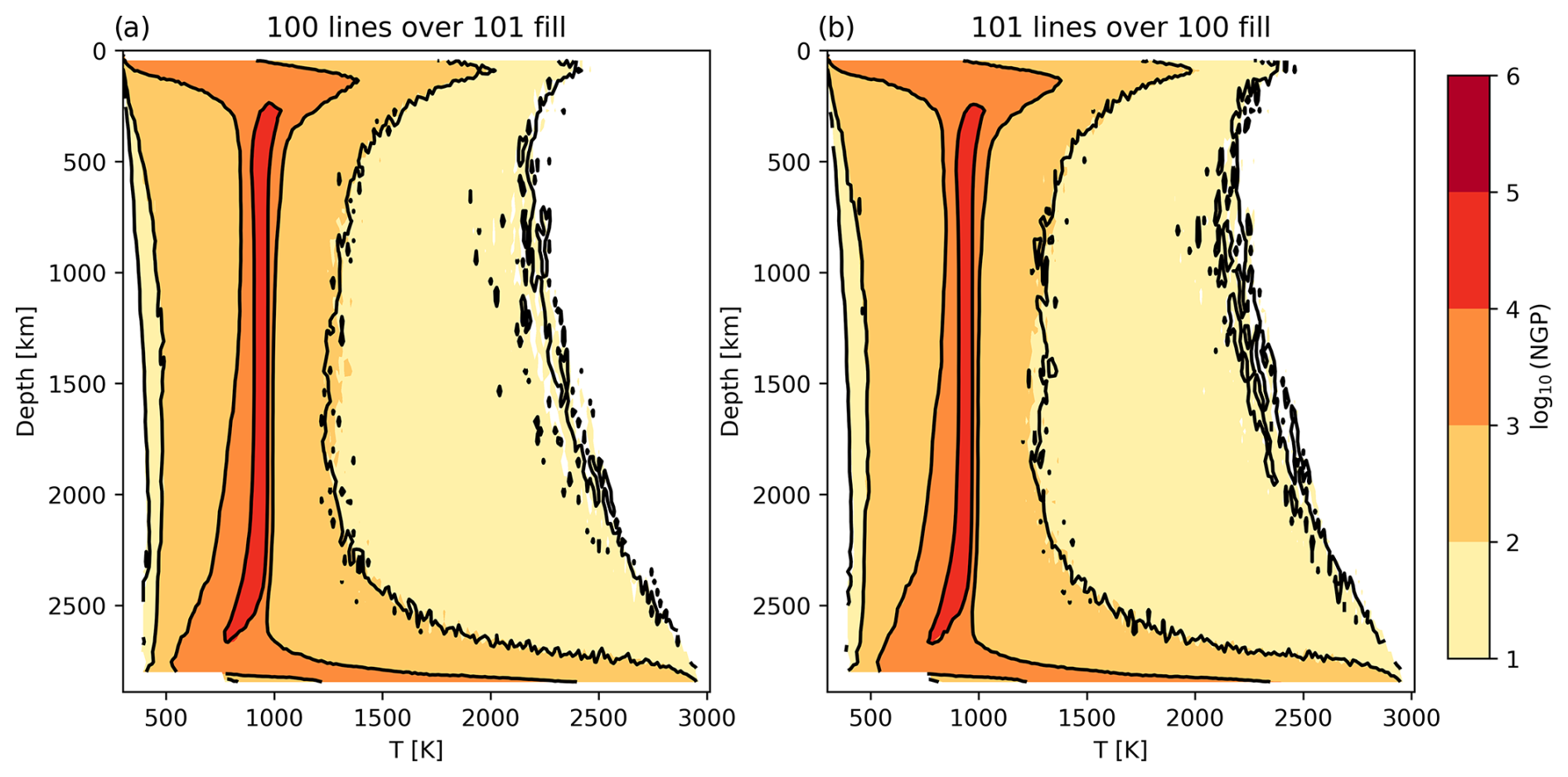
Figure A1 Radial temperature histograms coloured by number of grid points (“NGP”) for the reference case, Simulation number 100, and the akimotoite case, Simulation number 101, with contours of the reference (100) and Ak (101) simulations' radial temperature histograms overlaid respectively (a, b).

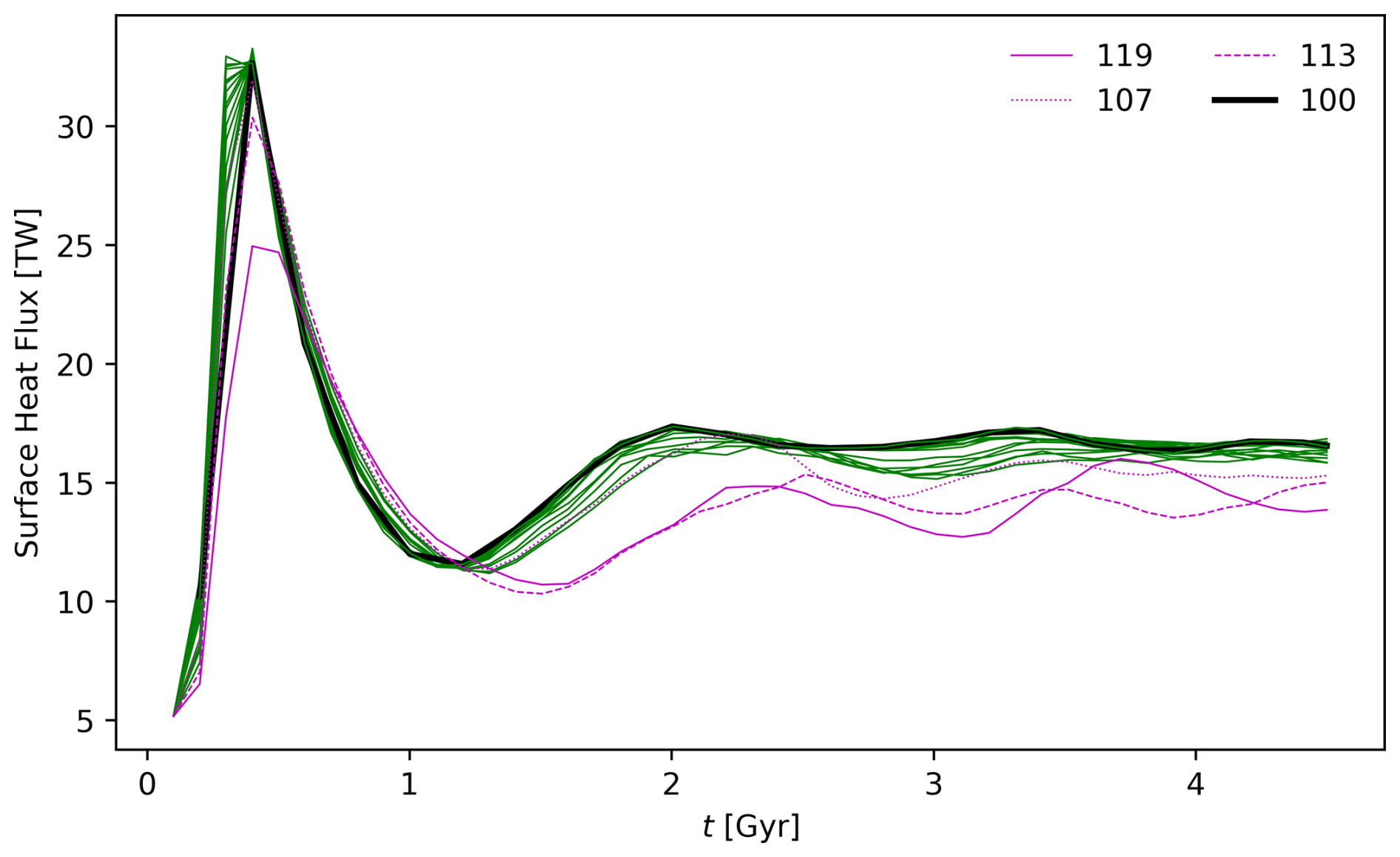
Figure A2 Evolution of surface heat flux of simple convection simulations in Table 2. Simulations are coloured according to their regime of convection in Fig. 7, with select simulations highlighted in legend – simulation 100 (the reference case) is shown by a heavy black line, and Simulation numbers 107, 113, and 119 are all in regime S (shown in magenta by dotted, dashed, and solid lines respectively). Other simulations (in regime W) are shown by the green line – see discussion of dynamic regimes in Sect. 2.6.2.

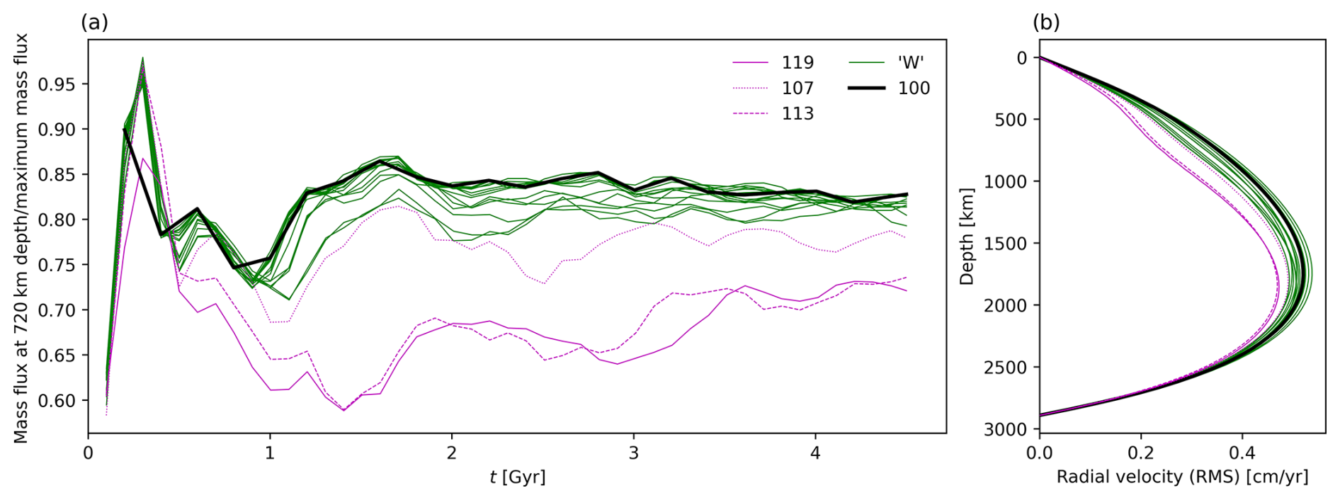
Figure A3 (a) Evolution of mass flux at 720 km depth of simple convection simulations in Table 2 and (b) End-of-simulation rms of radial velocity of simulations in Table 2. Simulations are coloured according to their regime of convection in Fig. 7, with select simulations highlighted in legend – simulation 100 (the reference case) is shown by a heavy black line, and Simulation numbers 107, 113, and 119 are all in regime S (shown in magenta by dotted, dashed, and solid lines respectively). Other simulations (in regime W) are shown by the green line – see discussion of dynamic regimes in Sect. 2.6.2.

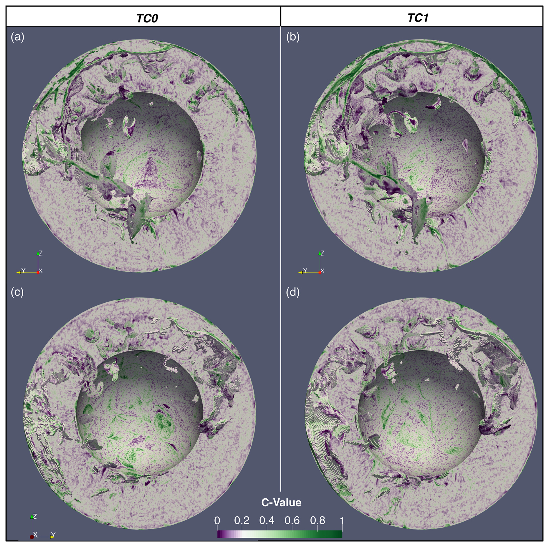
Figure A4 Comparison between reference MCM (TC0; a, c) and MCM with curved PGt phase transition morphology (TC1; b, d). C value, describing the composition between depleted (0, Harzburgitic), ambient (0.2, lherzolitic), and enriched (1, Basaltic) visualized on latitudinal slice through 90°, as well as on “voxels” beneath 500 K below the radial average temperature. Panels (a) and (b) show the Western Hemisphere, and panels (c) and (d) show the Eastern Hemisphere.