3D magnetotelluric forward modeling using an edge-based finite element method with a variant semi-unstructured conformal hexahedral mesh

This research presents the implementation of a semi-structured hexahedral mesh for the edge-based finite element method, which is utilized in solving 3D magnetotelluric (MT) modeling. The semi-unstructured conformal hexahedral mesh comprises an unstructured quadrilateral mesh for the horizontal directions and an automatically generated non-uniform mesh for the vertical direction. The edge-based finite element approach, utilizing this mesh pattern, has been developed. We present, compare, and discuss the accuracy, efficiency, and flexibility of our MT forward modeling codes for various 3D models. Numerical experiments indicate that our approach provides good accuracy when local mesh refinement is applied around sites and within the focus zone, yielding superior results compared to the conventional edge-based finite element method with a standard structured hexahedral mesh. The reliability of the developed codes was confirmed through comparisons with analytical solutions, benchmark COMMEMI3D, and topographic models. Furthermore, our developed codes, which incorporate a semi-unstructured conformal hexahedral mesh, exhibit valuable features, such as managing topographic and complex zones, and refining the local mesh for a 3D domain over a structured hexahedral mesh. However, they require fewer mesh data points, such as nodes and elements, within the mesh.

1 Introduction

3D Magnetotelluric (MT) forward modeling, the heart of 3D MT inversion, can be solved by many variant numerical techniques such as the integral equation (IE) approaches (Wannamaker, 1991; Avdeev et al., 1997; Avdeev, 2005), the staggered grid finite difference (SGFD) method (Mackie and Madden, 1994; Smith, 1996; Siripunvaraporn et al., 2002; Baba and Seama, 2002; Han et al., 2009), the edge-based finite element (EBFE) methods (Mitsuhata and Uchida, 2004; Nam et al., 2007; Liu et al., 2008; Han et al., 2009; Farquharson and Miensopust, 2011; Ren et al., 2013; Usui, 2015; Grayver and Kolev, 2015; Kordy et al., 2016; Zhang et al., 2021), the staggered-grid finite volume (SGFV) approaches (Haber et al., 2000; Haber and Ascher, 2001), and the hybrid finite difference-finite element (HFDFE) approach (Varılsüha, 2024). Their accuracy, efficiency, and validity have been presented, compared, and discussed. In the early era, the IE method using Green's function and the SGFD, which enforces current continuity (Yee, 1966; Siripunvaraporn et al., 2002), was accurate and efficient for simple 3D domains. For a more complex computational domain with topography, bathymetry, or irregular subdomains, computational loads increase dramatically because they rely more on the discretization or mesh to maintain the desired accuracy. Nevertheless, both IE and SGFD methods can, in theory, accurately model complex geometries like real-world ore bodies. The perceived restriction to rectangular discretizations is due to implementation decisions, not inherent mathematical limitations.

For such complex 3D models, the modeling problems can be mitigated by utilizing the EBFE, SGFV, or HFDFE methods due to the flexibility of mesh type. These methods can effectively handle domains, including those with irregular interior structures. These characteristics render the latter two techniques similar and powerful for implementation in real geophysical domains. The SGFV method, a numerical approach for various conservation laws, is particularly appealing when the numerical flux is significant (Eymard et al., 2000). However, research advancements in electromagnetic (EM) modeling for the SGFV approach still need to catch up to those of the variant EBFE method. For the HFDFE scheme (Varılsüha, 2020), implementing MT inversion still requires numerous additional verifications.

As mentioned, the flexibility and advantages of the EBFE method rely on the type of mesh used. The choice of mesh type for the EBFE approach has a significant impact on both the quality and cost of the solution (Tadepalli et al., 2011; Schneider et al., 2022). Tetrahedral meshes are advantageous due to their automated generation capabilities for even the most complex geometries. In rectangular meshes with brick elements, a common issue in simple rectilinear meshes is poor mesh quality, leading to system ill-conditioning. This problem occurs when padding zones extend to the domain boundary, creating very pizza-box-like cells. Hexahedral meshes are often regarded as the gold standard due to their significant improvements in accuracy and computational efficiency. This benefit comes from the structure of the brick element, which provides more precise results with fewer nodes and is less susceptible to numerical errors, such as shear and volumetric locking, that can affect simulations involving bending or incompressible materials. This improved accuracy per element offers a clear advantage, as simulations can use fewer elements to achieve the desired precision, resulting in smaller models, reduced memory usage, and faster solutions. Such efficiency is particularly crucial in various modeling applications. However, this high performance comes with a significant challenge, as creating high-quality hexahedral mesh is still a difficult and often manual process, highlighting a fundamental trade-off between optimal simulation performance and the ease of automating tetrahedral meshing. Presently, implementations of structured and unstructured hexahedral meshes have garnered significant attention, and numerous surveys and discussions have been presented (Owen, 1998). For MT, EBFE approaches using a structured hexahedral mesh have been given, and their performance has been investigated (Mitsuhata and Uchida, 2004; Nam et al., 2007; Kordy et al., 2016; Zhang et al., 2021). The variant EBFE method with adaptive non-conformal unstructured hexahedral mesh has also been presented (Grayver and Kolev, 2015; Grayver, 2015). However, the EBFE approach, incorporating a variant conformal hexahedral mesh, remains both interesting and challenging for achieving better performance in 3D inversion.

In this study, we present 3D MT forward modeling using an alternative EBFE approach that employs a semi-structured hexahedral mesh. The semi-structured mesh algorithm consists of two subprocesses. The mesh in the two horizontal directions is generated with an automatic unstructured quadrilateral mesh algorithm, while the vertical dimension is created using an automatic nonuniform mesh algorithm. The variational principle is then applied to the EEBFE approximation. Consequently, a direct solver from the Scipy library in Python is used to solve the resulting system of equations, and the responses are estimated. Finally, we evaluate and discuss the efficiency and accuracy of our approach across various models, including half-space, COMMEMI3D, and topographic models.

2 Governing equations

In MT modeling, the displacement currents are negligible, and the electric current source is free. Assuming a time dependence e^−iωt, the electromagnetic phenomena are described by the first-order Maxwell's equations:

$$\begin{array}{}\text{(1)}& {\displaystyle }& {\displaystyle }\mathrm{\nabla }\times \mathbf{E}=i\mathit{\omega }\mathit{\mu }\mathbf{H},\text{(2)}& {\displaystyle }& {\displaystyle }\mathrm{\nabla }\times \mathbf{H}=\mathit{\sigma }\mathbf{E},\end{array}$$

where E and H are the electric and magnetic fields, respectively, ω is the angular frequency, μ is the magnetic permeability of free space, and σ is the conductivity. Solving the above-coupled system requires large memory storage (Mackie and Madden, 1994; Siripunvaraporn et al., 2002). The memory storage can be reduced significantly by solving the second-order equations. A decoupled second-order Maxwell's equation for E is expressed as

$$\begin{array}{}\text{(3)}& \mathrm{\nabla }\times \mathrm{\nabla }\times \mathbf{E}=i\mathit{\omega }\mathit{\mu }\mathit{\sigma }\mathbf{E}\text{ in }\mathrm{\Omega },\end{array}$$

where Ω denotes the computing domain, including the air and earth layers.

At the boundaries of the computational domain, the tangential components of the electric field (Harrington, 2001; Liu et al., 2008) are required to satisfy

$$\begin{array}{}\text{(4)}& \mathit{n}\times \mathbf{E}=\mathit{n}\times {\mathbf{E}}_{\mathrm{0}}\text{ on }\mathrm{\Gamma },\end{array}$$

where Γ denotes the boundary of the computational domain, n represents the unit outward normal vector to the boundary, and E₀ denotes the primary electric field. In the present study, inhomogeneous Dirichlet boundary conditions are imposed by prescribing the tangential electric field components at Γ to be equal to the analytical magnetotelluric solution for a homogeneous or horizontally layered halfspace (Farquharson and Miensopust, 2011). This formulation is valid provided that the computational domain boundaries are sufficiently far from regions containing three-dimensional conductivity heterogeneities, so that the geoelectrical structure is effectively one-dimensional at the boundaries.

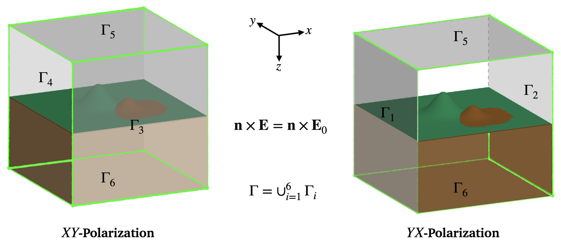
Figure 1 The boundary condition specifying on 3D domain for XY- and YX-polariztions. For XY-polarization, the tangential fields are specified on the front (Γ₃), back (Γ₄), top (Γ₅), and bottom sides (Γ₆). Otherwise, tangential fields are zeros. In contrast, for YX-polarization, the tangential fields are specified on the left (Γ₁), right (Γ₂), top (Γ₅), and bottom sides (Γ₆). Otherwise, tangential fields are zeros.

For magnetotelluric forward modeling, two orthogonal polarizations of the incident plane electromagnetic wave are considered. In the XY-polarization mode, the electric field is oriented parallel to the x-axis. Conversely, in the YX-polarization mode, the electric field is directed parallel to the y-axis. The complete magnetotelluric impedance tensor is subsequently obtained by solving the forward problem for both polarization modes independently and combining the resulting electromagnetic field solutions. The graphical representation is illustrated in Fig. 1.

3 Edge-based finite element method

3.1 Mesh algorithm: semi-unstructured conformal hexahedral mesh

The mesh generation or discretization of the computational domain is the first step in the EBFE approach to solve Eq. (3), subject to the boundary condition as in Eq. (4), which includes the EBFE approach. A continuous 3D model, Ω, was meshed into multiple subdomains or elements, i.e., $\mathrm{\Omega }={\cup }_{e=\mathrm{1}}^M{\mathrm{\Omega }}^e$, where Ω^e is the eth element and M is the total number of elements. For this work, all elements are hexahedra.

Generally, the MT domain Ω naturally composes air, irregular air-earth interfaces such as topography or bathymetry, and irregular subsurface with anomalies embedded within them. The structured hexahedral mesh can handle those by using a refinement mesh (Mitsuhata and Uchida, 2004; Nam et al., 2007; Kordy et al., 2016; Zhang et al., 2021). However, the refinement effects on the further subregions, i.e., the surplus small elements, appeared in the mesh. This also results in an excess of elements, and the distribution of the elements in the mesh does not smooth out as it should. This may result in a lower-quality mesh. Typically, producing high-quality mesh is essential for achieving optimal performance and accuracy in the FE Method when applied to the MT problem, as well-formed elements are crucial for stable numerical results and precise field representation (Jin, 2015).

In this work, we construct a semi-unstructured conformal hexahedral mesh for the 3D MT domain, comprising two main processes: an unstructured quadrilateral mesh generation for the surface and extrusion for the 3D volumetric domain. For the first process, the unstructured quadrilateral mesh can be generated by using direct and indirect approaches. An example of a direct approach, such as the paving algorithm and its application (Blacker and Stephenson, 1991), is the recent application of the paving algorithm to 2D MT domains presented in Sarakorn (2017). In contrast, the indirect approach is a well-established two-stage methodology that first generates a triangular mesh using robust algorithms such as Delaunay triangulation or advancing front methods, followed by systematic recombination of adjacent triangle pairs into quadrilateral elements (Bommes et al., 2013). This strategy decouples the geometric complexity of mesh generation from the topological optimization of element shape, leveraging the mathematical maturity and proven robustness of triangulation algorithms (Borouchaki et al., 1997) while achieving high-quality all-quad meshes through post-processing. Modern implementations employ sophisticated graph-theoretic recombination algorithms, most notably the Blossom-Quad method (Remacle et al., 2012), which formulates the triangle-pairing problem as a maximum-weighted perfect matching on the mesh dual graph and solves it optimally using Edmonds' blossom algorithm (Edmonds, 1965). This approach typically achieves 95 %–100 % quadrilateral coverage with superior element quality compared to simple greedy recombination heuristics (Owen et al., 1999), and has been successfully implemented in major mesh generation software, including Gmsh (Geuzaine and Remacle, 2009). Recent advances include the frontal-Delaunay method with an L^∞-norm Delaunay criterion (Remacle et al., 2013), which integrates advancing-front control with quad-oriented triangulation to improve mesh quality further and reduce the number of triangles requiring recombination. The indirect approach remains the dominant methodology for automatic quadrilateral mesh generation due to its robustness on complex geometries, excellent mesh-size control through background sizing fields (Frey and George, 2008), and its ability to handle arbitrary domain boundaries with minimal user intervention.

As discussed above, we introduce an adaptive unstructured quadrilateral surface-mesh generation algorithm specifically designed for MT modeling across large-scale geological domains with complex subsurface structures. The algorithm implements a hybrid indirect meshing approach that combines Delaunay triangulation with Blossom-Quad recombination (Remacle et al., 2012; Geuzaine and Remacle, 2009), enhanced by a unified multi-scale background mesh sizing field to address the unique challenges of MT forward modeling. The core methodology employs two refinement strategies operating simultaneously: edge-based refinement zones along geological layer boundaries and conductivity discontinuities, where acceptable mesh resolution is critical for accurate electromagnetic field computation, and point-based refinement zones centered at MT station locations and elevation refinement zones for existing terrain, ensuring adequate discretization near measurement sites while maintaining computational efficiency in the far field. A key innovation of our implementation is the use of smooth power-law transition functions with extended transition zones (controlled by an adjustable transition factor), which gradually vary element size from fine-scale regions to coarse far-field zones. This smooth gradation prevents abrupt changes in element size that would otherwise degrade mesh quality and introduce numerical errors in the finite element solution. The algorithm enforces a pure quadrilateral mesh requirement via aggressive topology optimization and iterative Laplacian smoothing (Bommes et al., 2013). After planar mesh generation, all nodes are projected onto the topographic surface $z=f(x,y)$ while preserving the mesh topology, enabling accurate representation of terrain effects on electromagnetic field propagation. The advantages of this approach for MT modeling include automatic handling of complex geological geometries across regional scales without manual intervention, more efficient multi-scale discretization with fewer elements compared to fine uniform meshes while preserving accuracy at key locations, guaranteed pure quadrilateral mesh output, smooth transitions in element size that reduce numerical dispersion and help maintain solution accuracy, and firm performance on domains with extreme aspect ratios and multiple refinement zones.

In summary, our mesh generation process of surface mesh can be composed as five main phases: geometry definition and topological construction, multi-scale mesh sizing field formulation, unstructured quadrilateral mesh generation with multiple strategies, surface projection to topography, and quality analysis and validation. The details of the algorithm for each phase are summarized in Appendix A. Remarkably, the unstructured quadrilateral mesh is generated by Gmsh (Geuzaine and Remacle, 2009), the open-source mesh generator, integrated with the Python environment. The obtained mesh data, including node coordinates and element connectivity, are then used in the second process, which extrudes the surface mesh into a 3D volumetric mesh for MT forward modeling in a Fortran 90/95 environment.

Starting from a surface mesh on Earth's surface (or Earth's seafloor if it exists), a 3D volumetric mesh with hexahedral elements is generated by vertically extruding the quadrilateral elements. Importantly, to accurately capture the significant resistivity contrasts and rapidly changing electromagnetic fields near the highly irregular topography and bathymetry, this extrusion uses an automatic, non-uniform layer thickness controlled by a fixed geometric transition rate. This adaptive vertical layering concentrates mesh resolution where it is most needed – near the complex air-earth interface and in other regions with expected high field gradients and penetration-depth effects (Simpson and Bahr, 2005) – without excessively increasing the total element count across the large-scale domain.

Figure 2 Example of meshing a 3D domain as a semi-unstructured conformal hexahedral mesh with linear elements.

Combining a flexible our algorithm for the horizontal plane with adaptive vertical layering enhances 3D MT modeling via the EBFE approach. It improves accuracy and efficiency by better handling electromagnetic fields within highly contrasting geophysical structures, which are crucial for accurate MT response simulation. The proposed concept of a semi-unstructured conformal hexahedral mesh with linear elements for the 3D MT domain is illustrated in Fig. 2.

3.2 Variational method

Once the meshing process is complete, the mesh information is used for the EBFE approximation in the next step. To construct the formula, the boundary value problems in Eq. (3) are expressed as the variational formula

$$\begin{array}{}\text{(5)}& \mathbf{F}(\mathbf{E},\mathbf{V})=g\left(\mathbf{V}\right),\mathbf{V}\in \mathbf{H}(\text{curl};\mathrm{\Omega }),\end{array}$$

where F is the bilinear form, H(curl;Ω) is the Sobolev space defined by $\mathbf{H}(\text{curl};\mathrm{\Omega })=\mathit{\{}\mathbf{V}\in L^{\mathrm{2}}(\mathrm{\Omega }{)}^{\mathrm{3}}:\mathrm{\nabla }\times \mathbf{V}\in L^{\mathrm{2}}\left(\mathrm{\Omega }{)}^{\mathrm{3}}\mathit{\right\}}$ (Monk, 2003) and V is the test function. Applying the algebraic vector properties and Green's theorem (Nam et al., 2007; Liu et al., 2008), the Eq. (5) can be deduced as

$$\begin{array}{}\text{(6)}& \mathbf{F}(\mathbf{E},\mathbf{V})=\underset{\mathrm{\Omega }}{\int }\left[(\mathrm{\nabla }\times \mathbf{E})\cdot (\mathrm{\nabla }\times \mathbf{V})-i\mathit{\omega }\mathit{\mu }\mathit{\sigma }\mathbf{E}\cdot \mathbf{V}\right]\mathrm{d}\mathrm{\Omega }.\end{array}$$

The Dirichlet boundary condition is regarded as the source term given by

$$\begin{array}{}\text{(7)}& \mathit{g}\left(\mathbf{V}\right)=\underset{\mathrm{\Gamma }}{\int }\mathbf{V}\cdot {\mathbf{E}}_{\mathrm{0}}\mathrm{d}\mathrm{\Gamma },\end{array}$$

where Γ is specified as the outer boundary of the domain. To solve the variational problem in Eq. (5), we discretize the domain Ω into distorted hexahedra, i.e.

$$\begin{array}{}\text{(8)}& \mathrm{\Omega }=\bigcup _{e=\mathrm{1}}^M{\mathrm{\Omega }}_e,\end{array}$$

where Ω^e is the eth hexahedral element and M is the total number of elements. The expression in Eqs. (6) and (7) can be expressed, respectively, as

$$\begin{array}{}\text{(9)}& {\displaystyle }& {\displaystyle }\mathbf{F}(\mathbf{E},\mathbf{V})=\sum _{e=\mathrm{1}}^M{\mathbf{F}}^e(\mathbf{E},\mathbf{V}),\text{(10)}& {\displaystyle }& {\displaystyle }\mathit{g}\left(\mathbf{V}\right)=\sum _{e=\mathrm{1}}^M{\mathit{g}}^e\left(\mathbf{V}\right),\end{array}$$

where

$$\begin{array}{}\text{(11)}& {\displaystyle }& {\displaystyle }{\mathbf{F}}^e(\mathbf{E},\mathbf{V})=\underset{{\mathrm{\Omega }}^e}{\int }\left[(\mathrm{\nabla }\times \mathbf{E})\cdot (\mathrm{\nabla }\times \mathbf{V})-i\mathit{\omega }\mathit{\mu }{\mathit{\sigma }}^e\mathbf{E}\cdot \mathbf{V}\right]\mathrm{d}\mathrm{\Omega },\text{(12)}& {\displaystyle }& {\displaystyle }{\mathit{g}}^e\left(\mathbf{V}\right)=\underset{{\mathrm{\Gamma }}^e}{\int }\mathbf{V}\cdot {\mathbf{E}}_{\mathrm{0}}\mathrm{d}\mathrm{\Gamma }.\end{array}$$

are defined over the Ω^e. For each Ω^e, the electric field is approximated by a linear combination of the basis functions given by

$$\begin{array}{}\text{(13)}& {\mathbf{E}}^e(x,y,z)=\sum _{i=\mathrm{1}}^{N^e}{\mathbf{W}}_i^e(x,y,z)u_i^e,\end{array}$$

where ${\mathbf{W}}_i^e(x,y,z)$ and $u_i^e$ denote the vector basis function and the tangential electric field, respectively, on the ith edge of the eth element, and N^e is the number of edge per element (here, N^e=12). The construction and expression of the vector basis functions for the hexahedral shape have been stated in several works (Volakis et al., 1998; Jin, 2015; Nam et al., 2007). Note that the construction of higher-order elements can be found in Grayver and Kolev (2015), and this can be applied to our mesh concept presented in this work. For this initiative, a first-order or linear element, as shown in Fig. 2 (right), is used.

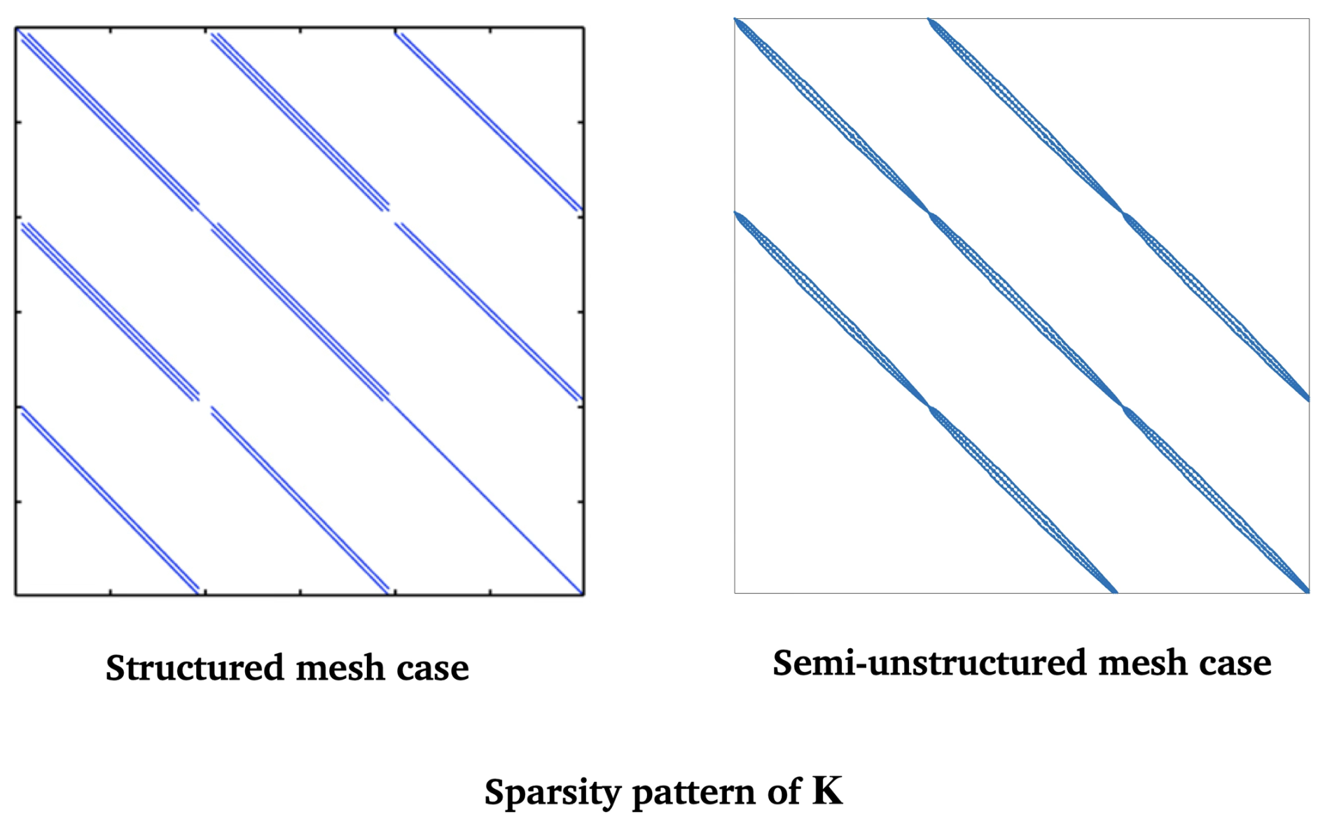
Figure 3 The example of sparsity pattern of some nonzeros in sparse matrices generated by the EBFE approach with a structured (left) and semi-unstructured (right) mesh.

The expression for each vector basis function is more complicated when expressed in Cartesian coordinates $(x,y,z)$. For simplicity, its expression will be expressed in the reference coordinate $(u,v,w)$ by using a coordinate transformation between the distorted hexahedron and a 2-unit cubic. To continue the procedure, we substitute Eq. (13) into Eq. (11) and then select the test function as a vector basis function. Rearranging terms, the final expression of the coefficients in Eqs. (11) and (12) is given by

$$\begin{array}{}\text{(14)}& {\displaystyle }\begin{array}{rl}{F}_{ij}^e=& \underset{{\mathrm{\Omega }}^{{}^{\prime }e}}{\int }\left[\left(\mathrm{\nabla }\times {\mathbf{W}}_i^e\right)\cdot \left(\mathrm{\nabla }\times {\mathbf{W}}_j^e\right)-i\mathit{\omega }\mathit{\mu }{\mathit{\sigma }}^e{\mathbf{W}}_i^e\cdot {\mathbf{W}}_j^e\right]\\ & \times \left|\mathbf{J}\right|\text{d}\mathrm{\Omega },\end{array}\text{(15)}& {\displaystyle }{g}_i^e=\underset{{\mathrm{\Gamma }}^{{}^{\prime }e}}{\int }{\mathbf{W}}_i^e\cdot {\mathbf{E}}_{\mathrm{0}}\mathrm{d}\mathrm{\Gamma },\end{array}$$

respectively. The appeared integrations are defined on reference coordinate, ${\mathrm{\Omega }}^{{}^{\prime }e}$ represents the 2-unit cubic, and ${\mathrm{\Gamma }}^{{}^{\prime }e}$ represents the corresponding face of the cubic. The notation $\left|\mathbf{J}\right|$ is denoted as the determinant of the Jacobian matrix of transformation. The numerical integration technique is used to approximate those formulas. Here, we use the Gauss quadrature rule, as in Nam et al. (Nam et al., 2007). To complete the FE procedure, we assembled all elements to obtain the linear system of equations

$$\begin{array}{}\text{(16)}& \mathbf{K}\mathit{u}=\mathit{g},\end{array}$$

where K is a large, sparse, symmetric, and complex matrix but not Hermitian, u is the unknown vector, and g is the source vector corresponding to the Dirichlet boundary conditions. If the structured hexahedral is incorporated, the raised coefficient matrix K has at most 33 nonzero elements per equation. However, the maximum nonzero value is unpredictable when the semi-unstructured mesh is imposed. It depends on the mesh generation and density in some focus zones. The example of the sparse matrices for the EBFE with a structured and semi-unstructured mesh is shown in Fig. 3. In practice, only nonzero elements are stored. The nonzero elements are stored by the Compressed Sparse Row (CSR) algorithm for our algorithm.

The system of equations in Eq. (16) can be solved using either Krylov subspace solvers with preconditioning (Nam et al., 2007; Smith, 1996; Mitsuhata and Uchida, 2004; Liu et al., 2008; Farquharson and Miensopust, 2011) or direct solvers (Kordy et al., 2016). Currently, efficient direct solvers for large, sparse linear systems from electromagnetic modeling are well established (Kordy et al., 2016; Shantsev et al., 2017) . Examples include the PARDISO (Schenk et al., 2001) and MUMPS (Amestoy et al., 2000; Shantsev et al., 2017) libraries. In this work, the MUMPS direct solver with an OpenMP interface is used instead of an iterative solver to prevent instability. Note that our coefficient matrix K in Eq. (16), stored in CSR format, is converted to COO format, which is standard for the MUMPS solver. The CPU time for the CSR-to-COO conversion is minimal and has no significant impact compared to the main factorization and substitution steps in the MUMPS solver (with observation, less than 0.05 %).

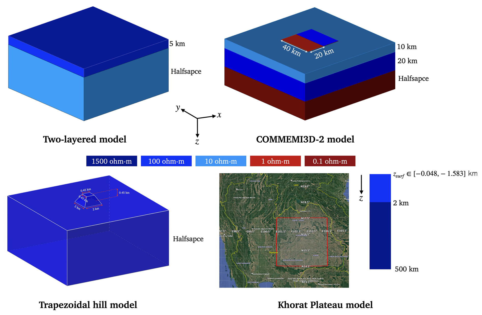
Figure 4 The 3D models used to validate and investigate the efficiency of our EBFE algorithm: two-layered model (top left), COMMEMI3D-2 model (top right), trapezoidal hill model (bottom left), and Khorat Plateau model (Source: Map data ©Google, Image© 2023 CNES/Airbus) (bottom right).

Once the solution to the linear system of equations is obtained, the electric field at each MT site can be approximated using Eq. (13). In contrast, the magnetic field can be approximated using Eq. (3). The impedance, the ratio of the electric to the perpendicular magnetic field, is then calculated for each station. The relationship of this quantity for 3D cases is defined by

$$\begin{array}{}\text{(17)}& \left[\begin{array}{cc}{E}_x^{xy}& E_x^{yx}\\ E_y^{xy}& E_y^{yx}\end{array}\right]=\left[\begin{array}{cc}{Z}_{xx}& Z_{xy}\\ Z_{yx}& Z_{yy}\end{array}\right]\left[\begin{array}{cc}{H}_x^{xy}& H_x^{yx}\\ H_y^{xy}& H_y^{yx}\end{array}\right],\end{array}$$

where the superscripts xy and yx are MT polarizations and the subscripts xx and yy are the horizontal components. The apparent resistivity and phase corresponding to the impedance can be calculated, respectively, by

$$\begin{array}{}\text{(18)}& {\mathit{\rho }}_{ij}^a={\displaystyle \frac{\mathrm{1}}{\mathit{\omega }\mathit{\mu }}}|Z_{ij}{|}^{\mathrm{2}},\end{array}$$

and

$$\begin{array}{}\text{(19)}& {\mathit{\varphi }}_{ij}=\text{arg}\left(Z_{ij}\right),\end{array}$$

where $i,j=x,y$, respectively.

4 Numerical results

This section will investigate the accuracy and efficiency of our EBFE approach with a semi-structured hexahedral mesh. The 3D models used here are the two-layered COMMEMI3D-2 model (Zhdanov et al., 1997), the trapezoidal hill model (Nam et al., 2007), and the Khorat Plateau model. The resistivity structures of the three models are shown in Fig. 4. Note that the air layer is always needed for all models and is included in each selected model. The thickness of the air layer is set as 100 km, and its resistivity is set as 10¹⁰ Ωm.

Figure 5 Comparison of structured (top row) and semi-unstructured (bottom row) hexahedral meshes for a two-layered model: 3D view (left), vertical cross-section view along the center (middle), and plan view (right) for the top and bottom of the domains. Note that the cross-section mesh of the two mesh types is set to be the same. The green line marks the interface between Earth's top and bottom layers, and the red cross indicates the locations of the stations.

4.1 Two-layered model

As shown in Fig. 4, this model assumes that the Earth's subsurface is flat, consisting of two layers. The thickness of the top and bottom layers is 5 km, and the half-space is 5 km thick. The corresponding resistivities are 100 and 10 Ωm, respectively. Therefore, the model's structure can be simplified to one dimension, allowing comparison of the numerical results with those of existing analytical solutions (Constable et al., 1987). To simulate the responses, the computational domain is set to 100 km × 100 km × 200 km (including the air layer). The 7 stations are designed to scatter from x− to x+ around the model's center, with a distance of 5 km between each (See Fig. 5). The EM wave periods used in this case are 0.1, 1.0, 10, and 100 s.

For the meshing model, the smallest element size, defined as the minimum edge length, is set to 30 m. The transition rate of element size in the z direction for the Earth's subsurface, the approximate ratio between adjacent element sizes, is set to 1.5 for both algorithms. In contrast, the transition rate for element size in the Air layer is set to 3 because the EM wave's skin depth is too considerable in air. These parameters played a crucial role in the methods' accuracy. The comparison between the two mesh types is shown in Fig. 5.

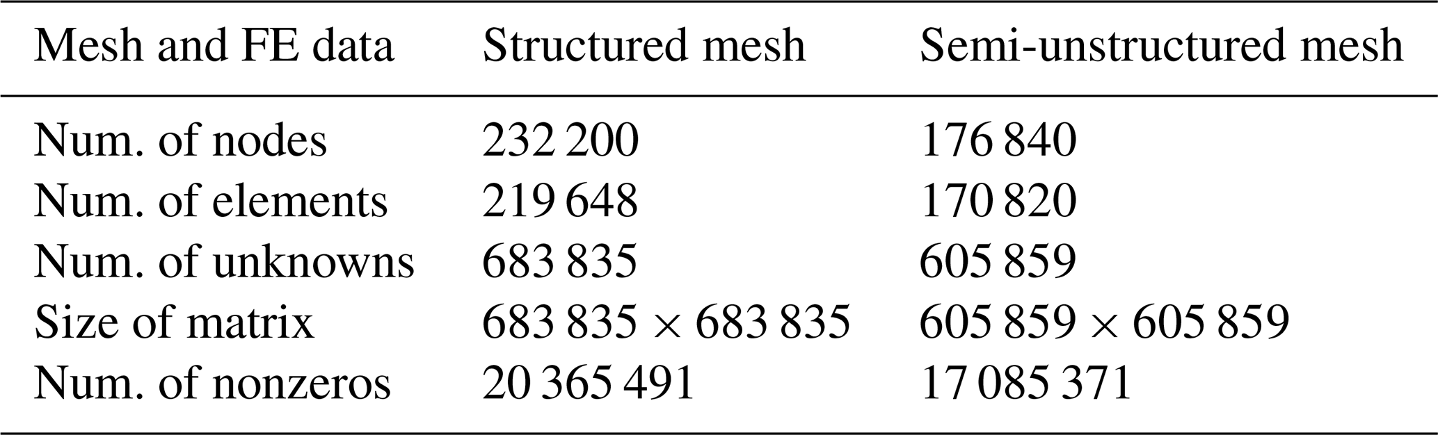
Table 1 Comparison of mesh information and EBFE data generated by structured and semi-unstructured conformal hexahedral mesh algorithms for the two-layered model.

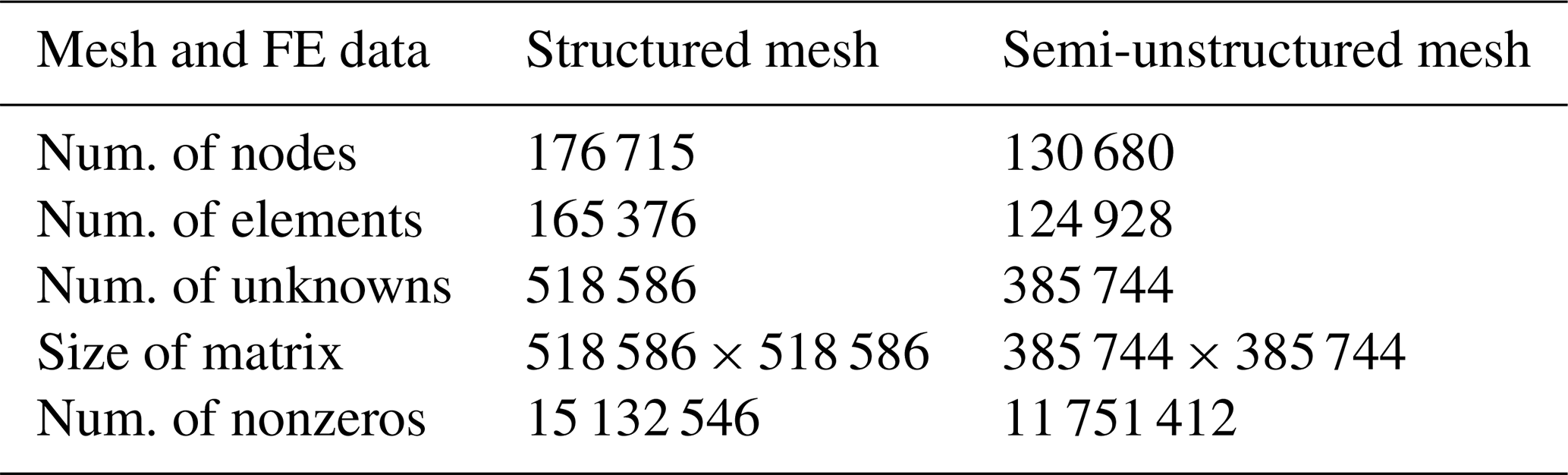
For the XY plane, both meshes around each station are refined to improve accuracy. As a result, the element density around and near each station is higher than in more distant regions. However, in the case of a semi-unstructured mesh created by a paving algorithm, the mesh's consistency is more flexible than that of a structured mesh generated by an automatic rectangular pattern. The mesh in the depth (z-direction) for both algorithms is identical for this research. The refinement is focused on the Earth's surface and the layer interface, similar to the case of the XY plane. The number of mesh sections from the top air layer to the bottom of the earth is 32 sections. The summary of the mesh information and EBFE data for each type is shown in Table 1.

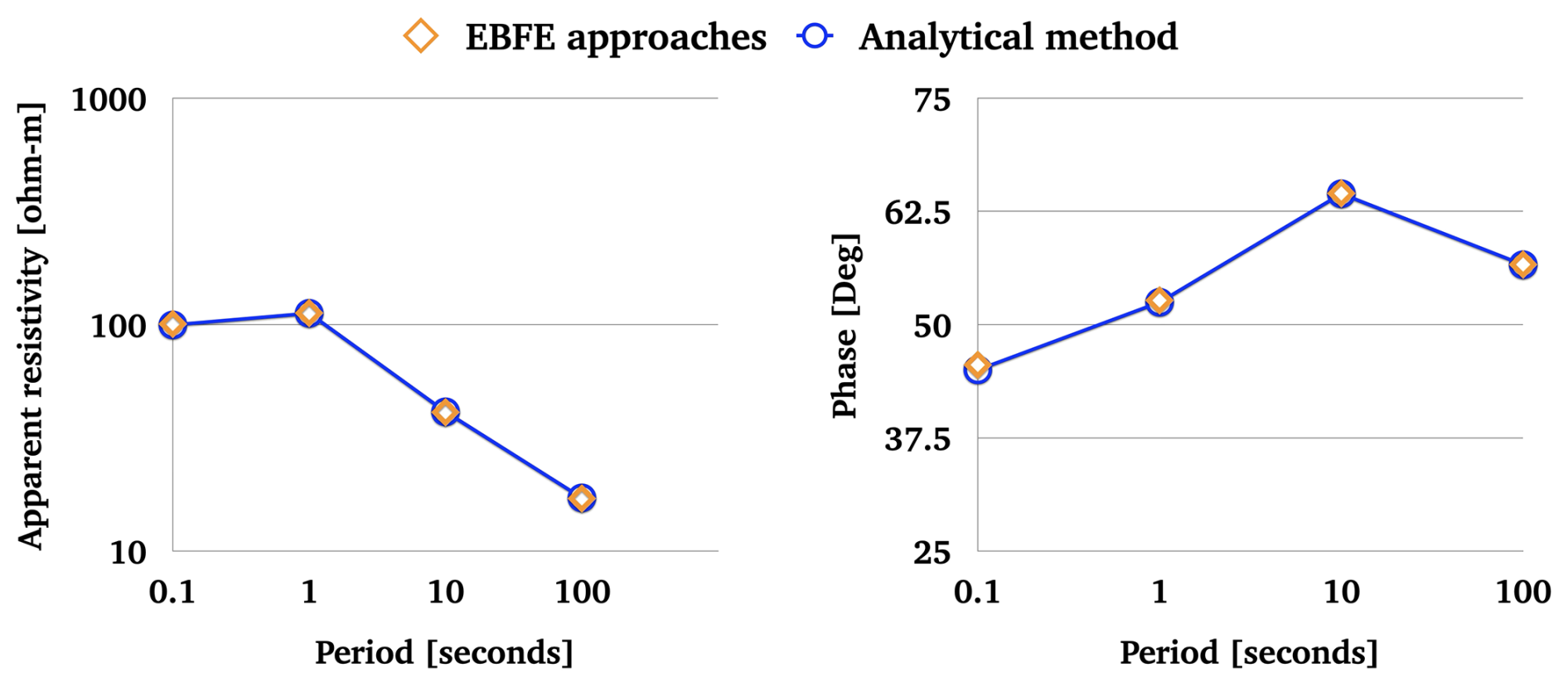
Figure 6 The comparison between the apparent resistivity and phase calculated by the EBFE with structured and unstructured hexahedral meshes and those by the analytical method. The maximum percentage of errors is less than 1 %.

With this condition, the density of elements in a structured hexahedral mesh is more significant than in a semi-unstructured conformal hexahedral mesh. Furthermore, the edge-based FEM with a structured mesh consumes more memory storage than the one with a semi-unstructured mesh.

The accuracy of the obtained apparent resistivity and phase at each edge-based finite element method period with structured and semi-unstructured mesh algorithms is measured as the Mean absolute percentage error (MAPE) . For this model, the errors obtained by the two approaches are identical because the model's structure is 1-D, as mentioned, and both algorithms use the same mesh in depth. The mesh in all horizontal directions does not affect the errors. Furthermore, the mistakes in responses and polarizations remain consistent throughout each period. Figure 6 shows the errors for each period. The MAPE at each period is less than 1 %.

Note that the apparent resistivity and phase of XY− and YX−polarizations and all vertical magnetic transfer function components are less than 10⁻²¹. Theoretically, these components are identical to zero for a 1-D structure (Simpson and Bahr, 2005). With the same level of accuracy, we observe that the EBFE approach with a semi-unstructured conformal hexahedral mesh uses significantly fewer computational resources, such as storage of nonzero entries in the coefficient matrix, as shown in Table 1, compared to the structured hexahedral mesh case, which is less than 22.34 %.

4.2 COMMEMI3D-2 model

The COMMEMI3D-2 model is one of several 3D models created by the COMMEMI projects (Zhdanov et al., 1997). As shown in Fig. 4, the COMMEMI3D-2 model assumes that the earth is flat and three-layered, with two anomalies embedded with different resistivities. The resistivity values for the top to bottom layers are 10, 100, and 0.1 Ωm, respectively. The thicknesses of the top and middle layers are 10 and 20 km, respectively. The bottom layer is semi-infinite. Two anomalies appeared embedded in the top layer with the exact sizes of 20 km × 40 km × 10 km. The resistivities for these two anomalies are 1 and 100 Ωm, respectively.

Figure 7 Meshing COMMEMI3D-2 model: Structured the hexahedral mesh is shown with a 3D view (top left), vertical cross-section at y=0 (top middle), and plan view (top right). The semi-structured mesh is displayed with a 3D view (bottom left), vertical cross-section at y=0 (bottom middle), and plan view (bottom right). The 15 red cross indicate the locations of stations.

To perform the forward calculation, the computing domain size is set as 200 km × 200 km × 200 km (air included). As with COMMEMI3D projects, the locations of 15 stations with meshing domain by two approaches are shown in Fig. 7.

Table 2 Comparison of mesh information and EBFE data generated by structured and semi-unstructured conformal hexahedral mesh algorithms for the COMMEMI3D-2model.

The mesh design still follows the same concept as the previous model, meaning that mesh refinement is applied around stations and interfaces, such as the air-earth interface and the anomaly-background interface. Additionally, local refinement is also implemented along the edges of the anomaly boundaries and around the station's location. In this case, the number of vertical mesh sections or layers is 39 in both the structured and semi-unstructured cases. The summary of the mesh information and EBFE data is shown in Table 2.

According to Table 2, the computational resources used by EBFE with a semi-unstructured mesh are still designed to be less than those used by EBFE with a structured mesh by about 16.11 %, to prove that the same accuracy level can be maintained for this model. Additionally, we present the CPU time required by each of our algorithms. The EBFE approach with a structured mesh takes 565 s for each polarization, which is longer than that of the EBFE approach with a semi-unstructured mesh, which takes 247 s. Note that this computation is performed on a MacBook Pro with Apple M1 Pro and 16 GB of RAM.

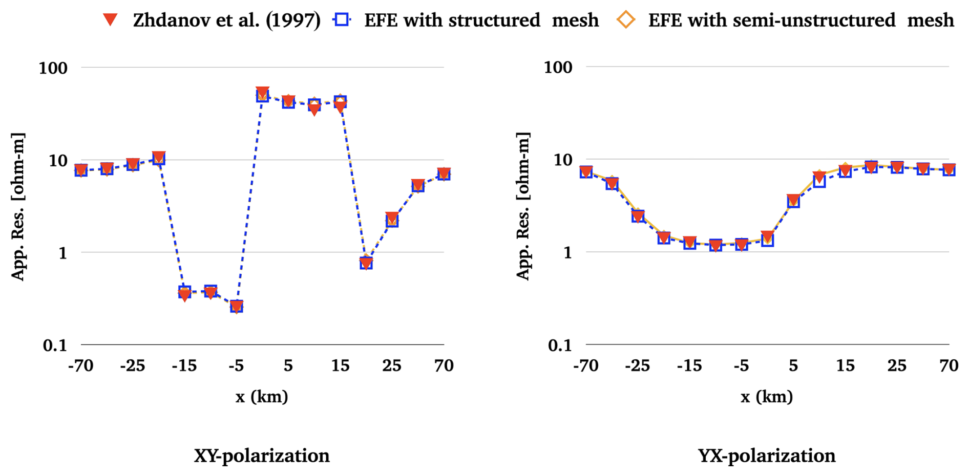
Figure 8 The comparison of apparent resistivity for XY−polarization (left) and YX−polarization (right) at period T = 1000 s.

The comparison of apparent resistivity at period $T=\mathrm{1},\mathrm{000}$ seconds estimated by our two approaches and the COMMEMI project is shown in Fig. 8. The graph of the MAPE is shown in Fig. 9. The MAPE from the two approaches for XY-polarization is higher than that for YX-polarization. For each polarization, the MAPE of the EBFE approach with a structured mesh is lower than that of the EBFE approach with a semi-unstructured mesh, with less significance.

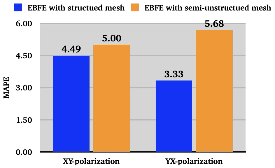
Figure 9 The calculated MAPE of apparent resistivity using the EBFE approach with structured and semi-unstructured data meshes.

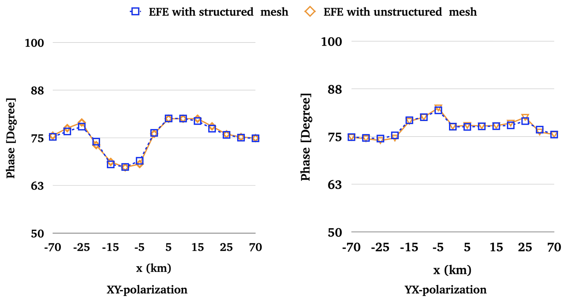
Figure 10 The comparison of phase for XY−polarization (left) and YX−polarization (right) at period T = 1000 s.

For the phase, the comparison of the apparent phase at a period of T = 1000 s, estimated by our two approaches, is shown in Fig. 10, while the COMMEMI projects do not present the phase in their experiments and are not shown in such a figure. When we compute the MAPE of the phases calculated by the EBFE approach using a semi-unstructured mesh, with the results from the structured mesh case as reference values, the obtained MAPEs are 0.60 % and 0.45 % for XY- and YX-polarizations, respectively, which are too low and show no significant difference.

With these metrics, the accuracy of our two approaches remains comparable, and their levels are nearly identical. However, the approach with a semi-unstructured mesh shows significantly better performance in terms of lower computational resource usage.

Figure 11 Meshing trapezoidal hill model: 3D view (top left), cross-section view at y = 0 km (top right), Earth's subsurface mesh (bottom left), and mesh around topographic zone (bottom right). The 41 red dots indicate the locations of stations.

4.3 Trapezoidal hill model

The 3D Trapezoidal hill model (Nam et al., 2007) is an extension of the 2-D case (Wannamaker et al., 1986). As shown in Fig. 4, the hill with a symmetric trapezoidal shape or truncated pyramid is designed at the center of the Earth's surface, whereas elsewhere it is flat. It has a rectangular base with 2 km × 2 km, top side with 0.45 km × 0.45 km, and with height 0.45 km. The resistivity structure is 100 Ωm halfspace. The meshing model using a semi-unstructured mesh is shown in Fig. 11. The refinement is imposed around size and topographic zone. Semi-structured mesh handles the topographic zone very well, and the mesh density around this zone is also relaxed. Note that the z-coordinate of each mesh point located beneath and above the topographic zone is adjusted to preserve the mesh projection at about depth $[-\mathrm{5},\mathrm{5}]$ km and the mesh refinement is similar to that on the boundary.

Figure 12 The comparison of responses at T = 0.5 s for trapezoidal hill model.

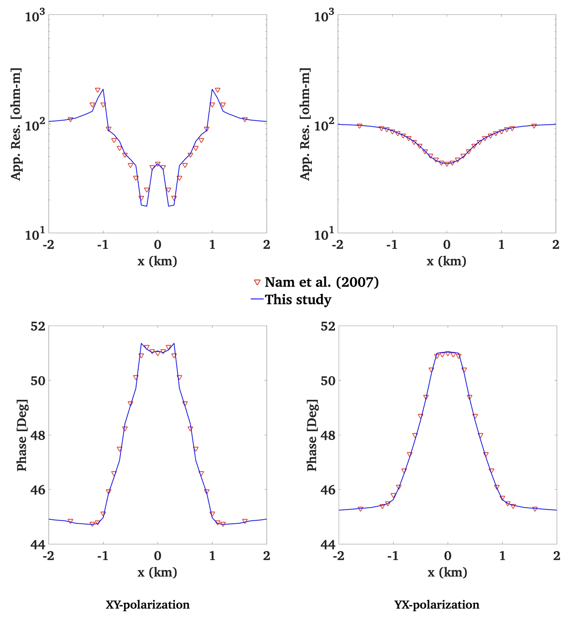
To perform the computing, the domain is set as 40 km × 40 km × 150 km (air included). The responses from 41 stations are computed at 0.5 s and compared to those of Nam et al. (2007). The responses are plotted, compared, and displayed in Fig. 12.

The results, the apparent resistivities and phase, indicate that the EBFE approach with a semi-structured mesh provides comparable responses to those calculated by the EBFE methods with a structured mesh (Nam et al., 2007).

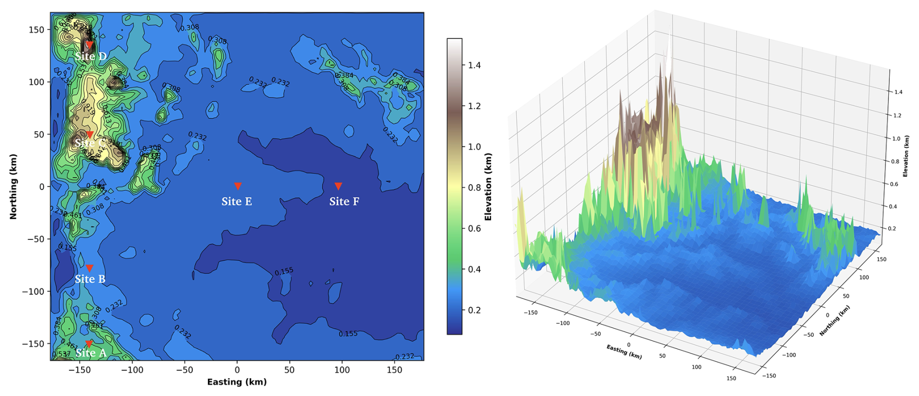
Figure 13 Khorat Plateau model: setting domain in red rectangle (top), contour of elevation (bottom left), estimated surface (bottom right). The six red triangles are the locations of sites A–F. Note that the z-direction is the positive upward with the sea level z = 0 km.

4.4 Khorat Plateau model

As shown in Fig. 4, this model is set in 14.5–17.5° N and 101.3–104.5° E, encompassing the Khorat Plateau, a saucer-shaped tableland in the Isan region of northeastern Thailand. The estimated elevation of the model with sample 150 × 150 points is shown in Fig. 13.

The domain covers 118 303.5 km², and the plateau exhibits considerable elevation variability depending on location and measurement method. The elevation range is approximately from 48 to 1583 m. The central part of the plateau consists of relatively monotonous plains, broken by gently rolling hills at approximately 150 m in altitude. However, the broader plateau region is generally situated between 90 and 200 m above sea level (z = 0 km). The terrain shows a topographic gradient from higher elevations in the northwest toward lower elevations in the southeast near the Mekong River. The Phu Phan Mountains divide the plateau into the northern Sakhon Nakhon Basin and the southern Khorat Basin. The Phetchabun bounds it, and Phang Hoei ranges to the west, the Phanom Dong Rak Range to the south, and the Mekong River along the northern and eastern borders with Laos. The Mun and Chi Rivers drain the plateau, both tributaries of the Mekong. The area has impermeable soils that flood seasonally from April to November and dry out afterward.

Currently, there is no published deep MT data for crustal structures in this region; we therefore have simplified it to a two-layer resistivity model to simulate the MT responses. The size of the computing domain is set as 355.8 km × 332.5 km × 600 km (air layer included). Note that the Easting and Northing are set to the x and y directions, respectively. To assign the resistivity structure, the top layer consists of a 2 km-thick sedimentary layer with ρ₁ = 100 Ωm, representing the Mesozoic Khorat Group, comprising sandstone, siltstone, and mudstone formations. The bottom layer, starting at depth z = 2 km, is set to a crystalline basement half-space with ρ₂ = 1500 Ωm, representing the felsic crust of the Indochina terrane. The sedimentary layer resistivity is constrained by near-surface electrical resistivity tomography surveys, which show values of 0–20 Ωm for clay-rich deposits and higher values for consolidated sediments (Nimnate et al., 2017). The crystalline basement resistivity is consistent with a felsic crustal composition, as indicated by receiver function studies showing Vp/Vs ratios of 1.74 ± 0.04 and a crustal thickness of 36.9 ± 3 km beneath the plateau (Noisagool et al., 2014; Yu et al., 2017). The location of six MT sites is shown in Fig. 13 (bottom left). Sites A, B, and D are located along the western margin with significant elevation relief, Site D in the northern highlands, and Sites E and F in the central basin.

Figure 14 Meshing on Khorat Plateau model: Earth's surface mesh (top left), plan view of Earth's surface mesh (top right), and vertical mesh section at x = −140 km and y=0 km with a zoom-in of the region of the highland (bottom).

The mesh of this domain with 256 127 nodes, 242 720 elements, and 749 902 unknowns is shown in Fig. 14. The top panels show the topographic surface as a 3D elevation view (left) and a plan-view mesh with adaptive refinement that responds to terrain complexity (right), where finer elements capture mountainous regions and coarser elements cover flat areas. The bottom panels display the complete 3D mesh extending to 500 km depth (left) and an enlarged cross-section (right) highlighting how hexahedral elements conform to the undulating terrain surface, demonstrating the integration of real topography into a structured mesh suitable for the EBFE method for EM modeling.

Figure 15 The estimated apparent resistivities and phase for sites A–F at T = 0.01–100 s of Khorat Plateau model: XY-polarizaton (firs column) and YX-polarization (second column).

The comparison of the estimated apparent resistivities and phase for sites A–F at T = 0.01–100 s is shown in Fig. 15. The trend of MT responses computed across the Khorat Plateau region matches the one-dimensional analytical solutions for both XY and YX polarizations during the test periods. Six measurement sites were strategically positioned across diverse topographic settings: Despite substantial topographic variations, all sites exhibit remarkably consistent with apparent resistivity increasing systematically from ∼ 100 Ωm at short periods to ∼ 1000 Ωm at long periods while phase responses display characteristic behavior with values near 45° at short periods, an inductive dip to ∼ 25° at intermediate periods (T = 1–10 s), and recovery toward 35–40° at more extended periods. The highest distortion appears at Site D (about 21 %), located in the highland, while the lowest distortion occurs at Site F (about 2 %), situated in the basin. This uniformity across geographically and topographically diverse locations indicates a relatively homogeneous regional electrical structure and validates the accuracy of our EBFE implementation, establishing a robust computational framework for subsequent magnetotelluric inversion studies in complex geological terrains.

5 Discussion

In this study, we presented and carefully evaluated an alternative edge-based finite element (EBFE) method for 3D magnetotelluric (MT) forward modeling, characterized by its innovative use of a semi-unstructured conformal hexahedral mesh. Our primary goal was to address ongoing challenges in 3D MT modeling, specifically balancing geometric flexibility, solution accuracy, and computational efficiency, especially when working with complex geological structures and the need for localized mesh refinement.

The proposed semi-unstructured conformal hexahedral mesh, which combines an unstructured quadrilateral mesh for the horizontal directions (created using the paving algorithm) with an automatically generated non-uniform mesh for the vertical direction, showed significant benefits. This hybrid meshing approach was crucial for achieving better mesh quality and adaptability compared to traditional structured hexahedral meshes. As shown by numerical experiments on the two-layered and COMMEMI3D-2 models, our method consistently used a notably lower number of nodes and elements, and consequently, fewer non-zero entries in the resulting coefficient matrix. Specifically, for the two-layered model, we observed about 22.34 % fewer nonzero data, and for the COMMEMI3D-2 model, roughly 16.11 % fewer, compared to the structured mesh versions (Tables 1 and 2). This reduction in mesh data directly decreases memory usage and accelerates computations, as further evidenced by the reduced CPU time for the COMMEMI3D-2 model (247 s with the semi-unstructured mesh versus 565 s with the structured mesh). The efficiency gains are primarily due to the targeted refinement capabilities of the semi-unstructured mesh, which limits the creation of “surplus small elements” in regions that do not require high resolution – an issue familiar with purely structured refinement methods.

Crucially, these efficiency improvements were achieved without compromising accuracy. For the 1D two-layered model, our approach yielded results with MAPE of less than 1 % (Fig. 6), identical to that of the structured mesh and in excellent agreement with analytical solutions. This confirms the fundamental correctness of the implementation even with reduced mesh density. For the more complex 3D model, COMMEMI3D-2 benchmark, the accuracy of our semi-unstructured EBFE method remained highly comparable to both the structured EBFE approach and established COMMEMI project results (Fig. 8). The computed MAPEs for phase, when referenced against the structured mesh case (0.60 % for XY-polarization and 0.45 % for YX-polarization), further underscore the negligible difference in accuracy between the two meshing strategies (Fig. 9). The successful validation against these well-known benchmarks confirms the reliability and robustness of our developed codes.

Furthermore, the flexibility of the semi-unstructured conformal hexahedral mesh was clearly demonstrated by its ability to effectively manage and conform to complex topographic features, as shown with the trapezoidal hill and Khorate Plateau models. As depicted in Figs. 11 and 14, our method efficiently handles irregular air-earth interfaces, offering a more relaxed and optimized mesh density around these critical areas. Unlike IE or SGFD methods, which are often implemented on rectangular discretization, our approach's adaptability makes it especially useful for realistic geophysical applications involving complex subsurface and surface geometries.

6 Conclusion

This research successfully developed and validated a 3D MT forward modeling approach utilizing an edge-based finite element (EBFE) method coupled with a novel semi-unstructured conformal hexahedral mesh. This meshing strategy, which combines unstructured quadrilaterals in the horizontal plane with non-uniform vertical layering, proved to be highly effective. Our numerical experiments consistently demonstrated that this approach maintains high accuracy, yielding results in excellent agreement with analytical solutions, established benchmark models, and comparative studies against topographic models. The EBFE approach achieves superior computational efficiency, notably by requiring fewer nodes, elements, and non-zero entries in the system matrix compared to conventional structured hexahedral meshes, leading to reduced memory consumption and faster computation times. Additionally, our EBFE method exhibits enhanced flexibility in handling complex geological features, including topographic variations and localized anomalous zones, through its adaptive mesh refinement capabilities without introducing unnecessary mesh density.

The reliability and performance demonstrated by our developed codes position this EBFE approach, featuring a semi-unstructured conformal hexahedral mesh, as a powerful and practical tool for advanced 3D MT forward modeling. Its ability to accurately and efficiently simulate MT responses in complex geological environments makes it an up-and-coming new option for future applications in 3D MT inversion, facilitating a more realistic and cost-effective interpretation of field data.

Appendix A: Adaptive unstructured quadrilateral surface Mesh algorithm with multi-scale refinement for MT Modeling

The adaptive unstructured quadrilateral surface Mesh algorithm with multi-scale refinement for MT modeling consists of five main phases as follows.

•  

  Phase 1: Geometry definition and topological construction.

•  

  Phase 2: Multi-scale mesh sizing field formulation.

•  

  Phase 3: Unstructured quadrilateral mesh generation with multiple strategies.

•  

  Phase 4: Surface projection to topography.

•  

  Phase 5: Quality analysis and validation.

A1 Phase 1: Geometry definition and topological construction

This phase builds the geometry and topology within the domain.

Algorithm A1 Algorithm of geometry construction.

Require:

Rectangular domain dimensions L_x,L_y, polygon set $\mathcal{P}=\mathit{\{}{P}_{\mathrm{1}},\mathrm{\dots },P_n\mathit{\}}$

Ensure:

Geometric model with topological entities

1:

Create domain boundary:

2:

$\mathcal{B}=\mathit{\left\{}\right(-L_x,-L_y),(L_x,-L_y),(L_x,L_y),(-L_x,L_y\left)\mathit{\right\}}$

3:

Create points $\mathit{\{}{b}_{\mathrm{1}},b_{\mathrm{2}},b_{\mathrm{3}},b_{\mathrm{4}}\mathit{\}}$ from ℬ

4:

Create lines $\mathit{\{}{l}_{\mathrm{1}},l_{\mathrm{2}},l_{\mathrm{3}},l_{\mathrm{4}}\mathit{\}}$ connecting boundary points

5:

Create outer curve loop Γ_outer from boundary lines

6:

Process embedded polygons:

7:

for each polygon P_i∈𝒫 do

8:

$V_i=\mathit{\{}{v}_{i,\mathrm{1}},\mathrm{\dots },v_{i,m}\mathit{\}}$ {Vertices of P_i}

9:

for each vertex $v_{i,j}\in V_i$ do

10:

Round coordinates: $v_{i,j}^{\prime }=\text{round}(v_{i,j}/\mathit{ϵ})\times \mathit{ϵ}$

11:

Check vertex map for duplicates

12:

if $v_{i,j}^{\prime }$ not in vertex map then

13:

Create geometric point p_i,j

14:

Store $v_{i,j}^{\prime }\to p_{i,j}$ in vertex map

15:

end if

16:

end for

17:

Create lines connecting polygon vertices

18:

Create curve loop Γ_i from polygon lines

19:

Create surface S_i from Γ_i

20:

Store polygon curves for refinement field

21:

end for

22:

Create domain surface:

23:

$S_{\text{outer}}=\text{PlaneSurface}({\mathrm{\Gamma }}_{\text{outer}},\mathit{\{}-{\mathrm{\Gamma }}_{\mathrm{1}},\mathrm{\dots },-{\mathrm{\Gamma }}_n\mathit{\left\}}\right)$

24:

Synchronize geometric model

Note that the tolerance ϵ is typically set to 10⁻³ to handle numerical precision in vertex coordinates while avoiding unnecessary duplication.

A2 Phase 2: Multi-scale mesh sizing field formulation

This phase employs a unified background mesh sizing field h(x) that combines the edge-based and point-based refinement strategies, defined by

$$\begin{array}{}\text{(A1)}& h\left(\mathbf{x}\right)=min\left(h_{\text{edge}}\right(\mathbf{x}),h_{\text{point}}(\mathbf{x}\left)\right),\end{array}$$

where h_edge and h_point are the combined edge-based and point-based refinement fields, respectively.

A2.1 Edge-based refinement

For each polygon P_i with target edge size $h_i^{\text{min}}$ and transition distance D_i, the edge-based refinement at the polygon i is defined by

$$\begin{array}{}\text{(A2)}& \begin{array}{rl}{h}_i^{\text{edge}}\left(\mathbf{x}\right)=& h_i^{\text{min}}+\left(h^{\text{max}}-h_i^{\text{min}}\right)\\ & \times min\left(\mathrm{1},{\left({\displaystyle \frac{d_i\left(\mathbf{x}\right)}{D_i}}\right)}^p\right),\end{array}\end{array}$$

where d_i(x) is the distance from point x to polygon boundary ∂P_i, h^max is the far-field mesh size, $D_i=\mathit{\alpha }\cdot h_i^{\text{min}}$ is the transition distance (α≈ 10–30), and p is the power parameter controlling transition curvature (p=1.5 for default). The combined edge refinement field is defined by

$$\begin{array}{}\text{(A3)}& h_{\text{edge}}\left(\mathbf{x}\right)=\underset{i=\mathrm{1},\mathrm{\dots },n}{min}{h}_i^{\text{edge}}\left(\mathbf{x}\right).\end{array}$$

A2.2 Point-based refinement

For each refinement zone R_j centered at c_j with fine size $h_j^{\text{fine}}$, coarse size $h_j^{\text{coarse}}$, and radius r_j, the point-based refinement at point j is defined by

$$\begin{array}{}\text{(A4)}& \begin{array}{rl}{h}_j^{\text{point}}\left(\mathbf{x}\right)=& h_j^{\text{fine}}+\left(h_j^{\text{coarse}}-h_j^{\text{fine}}\right)\\ & \times min\left(\mathrm{1},{\left({\displaystyle \frac{\Vert \mathbf{x}-{\mathbf{c}}_j\Vert }{r_j}}\right)}^p\right).\end{array}\end{array}$$

The combined point refinement field is defined by

$$\begin{array}{}\text{(A5)}& h_{\text{point}}\left(\mathbf{x}\right)=\underset{j=\mathrm{1},\mathrm{\dots },m}{min}{h}_j^{\text{point}}\left(\mathbf{x}\right).\end{array}$$

Algorithm A2 Algorithm of background mesh field construction.

Require:

Polygon curves with target sizes, refinement zones

Ensure:

Background sizing field h(x)

1:

ℱ=∅ {Field list}

2:

Edge refinement fields:

3:

for each polygon P_i with target size $h_i^{\text{min}}$ do

4:

$D_i=\mathit{\alpha }\cdot h_i^{\text{min}}$ {Transition distance}

5:

Create distance field $d_i=\text{Distance}(\partial P_i)$

6:

Create MathEval field:

7:

$f_i=h_i^{\text{min}}+(h^{\text{max}}-h_i^{\text{min}})\times min(\mathrm{1},(d_i/D_i{)}^p)$

8:

$\mathcal{F}=\mathcal{F}\cup \mathit{\left\{}{f}_i\mathit{\right\}}$

9:

end for

10:

Point refinement fields:

11:

for each refinement zone R_j at c_j do

12:

Create distance field d_j=Distance(c_j)

13:

Create MathEval field:

14:

$f_j=h_j^{\text{fine}}+(h_j^{\text{coarse}}-h_j^{\text{fine}})\times min(\mathrm{1},(d_j/r_j{)}^p)$

15:

$\mathcal{F}=\mathcal{F}\cup \mathit{\left\{}{f}_j\mathit{\right\}}$

16:

end for

17:

$h\left(\mathbf{x}\right)=min\mathit{\{}f\in \mathcal{F}\mathit{\}}$ {Combine all fields}

18:

Set h(x) as background mesh

A3 Phase 3: Unstructured quadrilateral mesh generation with multiple strategies

Phase 3 attempts multiple meshing strategies sequentially until a pure quadrilateral mesh is achieved. Each strategy combines a base triangulation algorithm with quad recombination.

Algorithm A3 Algorithm of multi-strategy unstructured quadrilateral mesh generation.

Require:

Geometric model, background field h(x)

Ensure:

Pure quadrilateral mesh ℳ

1:

Define strategy set 𝒮:

2:

S₁: Delaunay + Aggressive Optimization (algo=5, recomb=1, smooth=20, optimize=true)

3:

S₂: Frontal-Delaunay (algo=6, recomb=1, smooth=15, optimize=true)

4:

S₃: Automatic (algo=2, recomb=1, smooth=10, optimize=true)

5:

for each strategy S_k∈𝒮 do

6:

Clear existing mesh

7:

Set mesh algorithm parameters from S_k

8:

Set recombination options:

9:

RecombineAll = 1

10:

RecombinationAlgorithm = 1 {Blossom algorithm}

11:

SubdivisionAlgorithm = 1 {All-quad}

12:

RecombineOptimizeTopology = 5

13:

RecombineNodeRepositioning = 1

14:

Set smoothing iterations from S_k

15:

Disable boundary/point/curvature sizing:

16:

CharacteristicLengthExtendFromBoundary = 0

17:

CharacteristicLengthFromPoints = 0

18:

CharacteristicLengthFromCurvature = 0

19:

Set element size bounds:

20:

CharacteristicLengthMin = ${min}_i{h}_i^{\text{min}}$

21:

CharacteristicLengthMax = h^max

22:

Generate 2D mesh

23:

if mesh generation fails then

24:

continue to next strategy

25:

end if

26:

Count elements: n_quad, n_tri, n_total

27:

$q=n_{\text{quad}}/n_{\text{total}}$ {Quad percentage}

28:

if q=1.0 then

29:

return mesh ℳ {Success: 100 % quads}

30:

else

31:

continue to next strategy

32:

end if

33:

end for

34:

return failure {No strategy succeeded}

A3.1 Mesh quality settings

The quality of the mesh depends on key parameters. The main parameters for high-quality quad meshes are listed below:

1. Recombination Algorithm: Blossom-quad algorithm (Remacle et al., 2013) uses graph-matching theory to pair triangles into quadrilaterals optimally.

2. Topology Optimization Level 5: Aggressive reconnection and node relocation.

3. Node Repositioning: This parameter enables nodes to move to improve element quality.

4. Smoothing Iterations: Used for Laplacian smoothing.

5. Netgen Optimization: An additional optimization pass for element quality.

A4 Phase 4: Surface projection to topography

Once the planar mesh is generated in phase 3, all nodes are projected onto the topographic surface defined by $z=f(x,y)$. This approach preserves the mesh topology and element connectivity while adapting to varying terrain. In real scenarios where elevation data is available, a standard interpolation method is used to estimate f(x,y) before projection.

Algorithm A4 Algorithm of surface projection.

Require:

Planar mesh ℳ, surface function f(x,y)

Ensure:

Surface-conforming mesh ℳ^′

1:

Get all node tags and coordinates

2:

for each node i with coordinates $(x_i,y_i,z_i)$ do

3:

$z_i^{\prime }=f(x_i,y_i)$ {Compute surface elevation}

4:

if $|z_i^{\prime }-z_i|>\mathit{ϵ}$ then

5:

Update node coordinates to $(x_i,y_i,z_i^{\prime })$

6:

end if

7:

end for

A5 Phase 5: Quality analysis and validation

Algorithm A5 Algorithm of mesh quality analysis.

Require:

Mesh ℳ

Ensure:

Quality metrics

1:

Extract element connectivity and node coordinates

2:

Initialize element size array H=[]

3:

for each quadrilateral element e do

4:

Get vertices $\mathit{\{}{v}_{\mathrm{1}},v_{\mathrm{2}},v_{\mathrm{3}},v_{\mathrm{4}}\mathit{\}}$

5:

Compute edge lengths:

6:

${\mathrm{\ell }}_j=\Vert v_{j+\mathrm{1}}-v_j\Vert$ for $j=\mathrm{1},\mathrm{2},\mathrm{3},\mathrm{4}$ (cyclic)

7:

${\overline{h}}_e=\frac{\mathrm{1}}{\mathrm{4}}{\sum }_{j=\mathrm{1}}^{\mathrm{4}}{\mathrm{\ell }}_j$ {Average edge length}

8:

$H=H\cup \mathit{\left\{}{\overline{h}}_e\mathit{\right\}}$

9:

Compute element center (x_e,y_e)

10:

end for

11:

Compute mesh statistics:

12:

$h_{min}=min\left(H\right)$, $h_{max}=max\left(H\right)$, $\overline{h}=\text{mean}\left(H\right)$, σ_h=std(H)

13:

Size ratio (indicates the refinement effectiveness): $\mathit{\gamma }=h_{max}/h_{min}$

14:

Report:

15:

Element count, size range, mean, standard deviation

16:

Size ratio

A size ratio γ>2 typically indicates successful multi-scale refinement, while γ>10 demonstrates significant adaptive refinement.